Revisiting $\ell_{1}$ Loss in Super-Resolution: A Probabilistic View and Beyond

Abstract

Super-resolution as an ill-posed problem has many high-resolution candidates for a low-resolution input. However, the popular $\ell_{1}$ loss used to best fit the given high-resolution image fails to consider this fundamental property of non-uniqueness in image restoration. In this work, we fix the missing piece in $\ell_{1}$ loss by formulating super-resolution with neural networks as a probabilistic model. It shows that $\ell_{1}$ loss is equivalent to a degraded likelihood function that removes the randomness from the learning process. By introducing a data-adaptive random variable, we present a new objective function that aims at minimizing the expectation of the reconstruction error over all plausible solutions. The experimental results show consistent improvements on mainstream architectures, with no extra parameter or computing cost at inference time.

I Introduction

The behavior of single image super-resolution (SISR) networks is primarily driven by the choice of the objective function. Two common examples in SISR are the mean squared error (MSE) loss and the mean absolute error (MAE) loss. Since the long-tested measure peak signal-to-noise ratio (PSNR) is essentially defined on the MSE, pioneer works [1, 2, 3, 4, 5, 6] have largely focused on minimizing the mean squared reconstruction error to achieve high performances.

Due to the ill-posed nature of SISR problem, a low-resolution image $\mathbf{x}$ can be well described as the downsampling result of many high-resolution images $\mathbf{\hat{y}}_{1:k}$. This implies that, in the inverse image reconstruction, the neural network trained by MSE loss, i.e., $\mathbb{E}_{(\mathbf{x},\mathbf{\hat{y}})}[\sum_{i}\|f(\mathbf{x})-\mathbf{\hat{y}}_{i}\|_{2}^{2}]$, will learn to output the mean value of all HR targets, i.e., $f(\mathbf{x})\rightarrow\frac{1}{k}\sum_{i}\mathbf{\hat{y}}_{i}$, which best fits the image pairs $\{\mathbf{x},\mathbf{\hat{y}}_{1:k}\}$ [7]. However, the average of different HR images results in the absense of distinct edges and the blurring effect, which suffers from low image fidelity despite relatively high PSNR. Recently, $\ell_{1}$ loss has received much attention from low-level vision researches, since it is in practice more robust to the regression-to-the-mean problem in MSE loss [8, 9]. Despite its emprical success in state-of-the-arts super-resolution methods [10, 11, 12, 13, 14, 15], $\ell_{1}$ loss itself has been rarely discussed in the context of image processing.

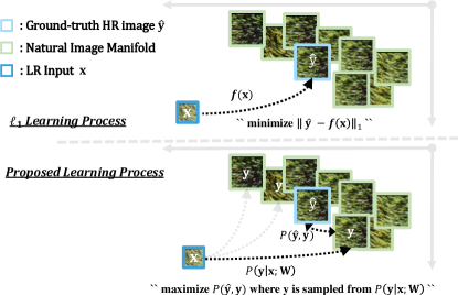
Figure 1: Illustration of the learning process given an LR-HR image pair. $\ell_{1}$ loss only considers the fitting error between model output $f(\mathbf{x})$ and HR image $\mathbf{\hat{y}}$. We propose to learn an one-to-many mapping by introducing $P(\mathbf{y}|\mathbf{x};\mathbf{W})$ explicitly: 1) first perform a random sampling from $P(\mathbf{y}|\mathbf{x};\mathbf{W})$ to obtain a underlying natural image $\mathbf{y}$; 2) then maximize the likelihood of $\mathbf{y,\hat{y}}$ co-occurrence. Since we focus on the expected value averaged across all $\mathbf{y}$ instead of any specific sampling result, the learning process serves as a multiple-valued mapping.

In probabilistic setting, it is well known that a median is the minimizer of $\ell_{1}$ loss with respect to given targets [16]. In the case of training neural networks over LR-HR image pairs, the situation is quite similar to MSE loss where the network will learn to recover the median of all perceptually convincing HR images $\mathbf{\hat{y}}_{1:k}$. However, both $\ell_{1}$ and $\ell_{2}$ loss only capture the median/mean value of the whole solution space, which can be inadequate for estimating any specific solution in high-dimensional predictions, super-resolution in particular.

In this paper, we begin with a simple idea that it is intuitive to learn a one-to-many mapping since there are plenty of perceptually convincing solutions to an LR input (shown in Figure 1). Ideally, we may approximate the local manifold, corresponding to the ground-truth HR image, by the posterior distribution $P(\mathbf{y}|\mathbf{x};\mathbf{W})$. Notice that, generative methods are able to capture the more complex distribution of natural images, which inspires us to revisit super-resolution with neural networks from a probabilistic view. In this way, we have the following contributions:

• We derive a loss function for solving SISR by introducing a posterior Gaussian distribution of underlying natural image $\mathbf{y}$, i.e., $P(\mathbf{y}|\mathbf{x};\mathbf{W})$, which minimizes the expected reconstruction error across all plausible solutions in $\mathbf{y}$. The formulated learning process can be easily extended to other $P(\mathbf{y}|\mathbf{x};\mathbf{W})$ with different distributions such as Laplace.

• The learned standard deviation of $P(\mathbf{y}|\mathbf{x};\mathbf{W})$ facilitates the HR image regression and, as a by-product, allows us to make meaningful estimates of the model uncertainty in SISR, i.e., a way to reflect its SR correctness likelihood. This can be useful in settings where errors carry serious repercussions such as medical image super-resolution.

• The experimental results show consistent improvements over popular $\ell_{1}$ loss on mainstream networks, without the extra cost at runtime.

II Related Work

Super-resolution Over the past decades, super-resolution is among the most fundamental low-level vision problems. Early works often formulate the task as an interpolation [17, 18, 19, 20]. Latter studies start to reconstruct high-resolution images in a data-driven way, by estimating the natural image statistics [21, 22] (including deep prior [23, 24]) and exploiting the neighbor embedding [25, 26, 27]. Another group of methods utilizes the self-similarities to learn the inverse mapping [28, 29, 30, 31]. Benefiting from the development of sparse coding, [32, 33, 34] achieve reasonable results on benchmark datasets.

Advances in deep learning have further enhanced the state-of-the-art performance since [1, 3] first introduce a CNN-based SR method. Various CNN architectures have been proposed such as residual networks [35, 2, 9], densely connected networks [36, 37], ode-inspired design [38] and U-Net encoder-decoder networks [39, 40, 41]. In particular, the attention mechanism has become a popular tool for image super-resolution. Both channel attention [10] and non-local technique [12, 11] achieve notable improvements over baseline methods. Recently, self-correlation/self-attention that models the long-distance relationship among similar patches have led to successful results [15, 13, 42], as the large training dataset can be used as a means to capture the global information [43, 44, 45]. Our approach can facilitate the training of deep learning-based methods in a plug-in and play manner.

Loss functions Most learning objects in the literature fall into two main categories: pixel-wise loss and perceptual loss. The former aims to optimize the full reference metric such as PSNR and SSIM. MSE loss, in particular, is equivalent to PSNR. However, [46, 47, 48] show that $\ell_{2}$ loss results in overly-smooth SR images and the following works tend to use $\ell_{1}$ during training. In light of the success of knowledge distillation in image recognition, [49, 50] use loss functions in the feature space to enhance the performance of student networks. Our work also falls into this category. We propose to learn from a posterior distribution instead of best-fitting ground-truth images.

Perceptual loss tackles the problem by employing generative adversarial networks [48, 51], especially in super-resolution with large upscaling factors (e.g., $4\times$, $8\times$) [52, 6]. The ImageNet pre-trained networks are commonly used as a discriminator loss [47, 46, 24], which leads to high-frequency details and perceptually satisfying results in the sense. Our approach can be compatible with those adversarial settings as the content loss term in a perceptual loss.

The most related work is Noise2noise [53], which suffers from inaccurate gradient directions (details in Section III-C). We solve this problem by a well-bounded gradient step and point out that [53] indeed serves as a special case of our approach. Noise2Self [54] assumes that noise in each patch is independent of other patches, which can not hold responsible when it comes to the content of images instead of noise. Self2Self [55] presents dropout in both image and feature space to reduce prediction variances, which is also compatible with our loss functions.

Model uncertainty Despite their unprecedented power to solve the inverse problem, deep learning-based SR methods are prone to make mistakes. As deep models are widely used in computer-aided diagnosis [56, 57], it is crucial to better understand the confidence of neural networks in their predictions. That is, the SR network may provide uncertainty about the generated super-resolved images: which part is “real” and when we should be cautious.

[58] first develops a framework for modeling uncertainty, which is hard to describe the modern deep neural networks. Recently, Monte Carlo Dropout [59] presents a practical solution to estimate uncertainty via the dropout layer. [60] further shows that networks trained with Batch-Normalization [61] (BN) is an approximate Bayesian model and allows an uncertainty estimation by sampling the network’s BN parameters. Unfortunately, neither of them was used in recent SR networks, which disables the variational inference in those approximate Bayesian models. Instead, we model the posterior distribution $P(\mathbf{y}|\mathbf{x};\mathbf{W})$ explicitly, as a by-product, the estimated standard deviation facilitates the uncertainty estimation for SISR.

III Analysis

III-A Probabilistic Modeling

From a statistical viewpoint, we are interested in the point estimation of the model parameters $\mathbf{W}$, used in the following likelihood function:

$$\max_{\mathbf{W}}\ \mathcal{L}(\mathbf{W}|\mathbf{\hat{y}})=P(\mathbf{\hat{y}}|\mathbf{x};\mathbf{W})$$ (1)

where $\mathbf{W}$, $\mathbf{\hat{y}}$ and $\mathbf{x}$ indicate weights, observed ground-truth labels and inputs respectively. Super-resolution using convolutional neural networks also fall into this form, that learning parameters $\mathbf{W}$ w.r.t. an inference function $f(\mathbf{x})$ from LR-HR image pairs directly.

In contrast to finding a one-to-one mapping between corrupted images and targets implied by $f(\mathbf{x})$, we begin with a subtle point: in reality, the mapping from $\mathbf{\hat{y}}$ to $\mathbf{x}$ is surjective. For example, a single LR image $\mathbf{x}$ may correspond to the downsampling result of multiple natural images. Hence, it is intuitive to recover or approximate the local image manifold instead of simply fitting the high-resolution image $\mathbf{\hat{y}}$.

Objective function The idea is to explicitly estimate a posterior distribution $P(\mathbf{y}|\mathbf{x};\mathbf{W})$ where $\mathbf{y}$ refers to (multiple) underlying natural images with the size of $H\times W$. Then, the observed HR image $\mathbf{\hat{y}}$ should look like its counterpart $\mathbf{y}$ sampled from $P(\mathbf{y}|\mathbf{x};\mathbf{W})$, with high probability. Formally, our goal is to maximize the following conditional joint density function:

$$P(\mathbf{\hat{y}},\mathbf{y}|\mathbf{x};\mathbf{W})=P(\mathbf{\hat{y}|y})P(\mathbf{y}|\mathbf{x};\mathbf{W})$$ (2)

where $P(\mathbf{\hat{y}|y})$ is a measure of the probability that $\mathbf{\hat{y}}$ being observed given $\mathbf{y}$. Note that, there are plenty of $\mathbf{y}$ can serve as the perceptually convincing solution to Equation (2) then, as is common in machine learning, we take the expectation of that formula to be optimized:

$$\mathbb{E}_{\mathbf{y}\sim P(\mathbf{y}|\mathbf{x};\mathbf{W})}[P(\mathbf{\hat{y}|y})].$$ (3)

To solve Equation (3), we will first need to deal with $P(\mathbf{y}|\mathbf{x};\mathbf{W})$, the distribution of underlying natural images $\mathbf{y}$ consistent with the low-resolution $\mathbf{x}$.

Optimizing the objective Based on the finding of non-local means [62, 63] that each pixel is obtained as a weighted average of pixels centered at regions similar to the reference and the central limit theorem (CLT), we shall model $P(\mathbf{y}|\mathbf{x};\mathbf{W})$ as a multivariate normal distribution:

$$P(\mathbf{y}|\mathbf{x};\mathbf{W})\sim\mathcal{N}(\bm{\mu}_{(\mathbf{x};\mathbf{W})};\bm{\Sigma}_{(\mathbf{x};\mathbf{W})})$$ (4)

where mean $\bm{\mu}$ and covariance $\bm{\Sigma}$ are outputs of multi-layer neural networks with parameters $\mathbf{W}$. $\bm{\sigma}^{2}$ corresponds to the diagonal elements in $\bm{\Sigma}$. However, the expectation in Equation (3) still involves sampling $\mathbf{y}$ from $P(\mathbf{y}|\mathbf{x};\mathbf{W})$ which is a non-differentiable operation. To allow the backprop through $\mathbf{y}$, we use one of the most common trick in machine learning, the “reparameterization” [64], to move the sampling to the random variable $\mathbf{z}\sim\mathcal{N}(\bm{0},\bm{1})$:

$$\mathbb{E}_{\mathbf{y}\sim P(\mathbf{y}|\mathbf{x};\mathbf{W})}[P(\mathbf{\hat{y}|y})]=\mathbb{E}_{\mathbf{z}\sim\mathcal{N}(\bm{0},\bm{1})}[P(\mathbf{\hat{y}|\bm{\mu}+\bm{\sigma}*z})]$$

where $\mathbf{y}$ is reformulated as $\bm{\mu}+\bm{\sigma}*\mathbf{z}$ and “$*$” indicates elementwise product. Then, we can conduct the standard gradient descent and the gradient averaged over $\mathbf{z}$ should converge to the actual gradient of Equation (3).

Similarly, as [24], we consider the conditional model defined by the Gibbs distribution (also known as Boltzmann distribution):

$$P(\mathbf{\hat{y}|y})\varpropto\prod_{i}^{H\times W}\mathrm{exp}(-\frac{|\mathbf{\hat{y}}_{i}-\mathbf{y}_{i}|}{kT})$$ (5)

where the corresponding Gibbs energy is in the form of $\|\mathbf{\hat{y}}-\mathbf{y}\|_{1}$ and $kT$ is the fixed partition function. The model (5) assumes that $\mathbf{y}$, looks like the observed ground-truth image $\mathbf{\hat{y}}$, is likely to be a strong evidence for $\mathbf{\hat{y}}$ occurring. We can now get both $P(\mathbf{y}|\mathbf{x};\mathbf{W})$ and $P(\mathbf{\hat{y}|y})$ into Equation (3) then apply negative log-likelihood to the final objective for computational convenience:

$$\min\ \mathbb{E}_{\mathbf{z}}\Big{[}\frac{1}{kT}\sum_{i}^{H\times W}|\mathbf{\hat{y}}_{i}-(\bm{\mu}_{i}+\bm{\sigma}_{i}*\mathbf{z})|\Big{]}.$$ (6)

This equation implies a two-branch network ($\bm{\mu}$ and $\bm{\sigma}$) that requires randomness during training. The expectation on the data-independent random variable $\mathbf{z}$ allows us to move the gradient symbol into the expectation to finish the standard stochastic gradient descent [65]. For notational simplicity, we shall in the remaining text denote Equation (6) as $\mathbb{E}_{\mathbf{z}}\Big{[}\|\mathbf{\hat{y}}-(\bm{\mu}+\bm{\sigma}*\mathbf{z})\|_{1}\Big{]}$.

III-B Revisiting $\ell_{1}$ Loss

According to Jensen’s inequality, for any measurable convex function $f(\cdot)$, we have $\mathbb{E}[f(\mathbf{z})]\geq f(\mathbb{E}[\mathbf{z}])$. Since every $p$-norm is convex and $\mathbf{z}\sim\mathcal{N}(\bm{0},\bm{1})$, then we have

$$\mathbb{E}_{\mathbf{z}}\Big{[}\|\mathbf{\hat{y}}-(\bm{\mu}+\bm{\sigma}*\mathbf{z})\|_{1}\Big{]} \geq\|\mathbf{\hat{y}}-(\bm{\mu}+\bm{\sigma}*\mathbb{E}_{\mathbf{z}}[\mathbf{z}])\|_{1}$$ (7)

Considering $\mathbb{E}_{\mathbf{z}}[\mathbf{z}]=0$, then

$$\mathbb{E}_{\mathbf{z}}\Big{[}\|\mathbf{\hat{y}}-(\bm{\mu}+\bm{\sigma}*\mathbf{z})\|_{1}\Big{]}\geq\|\mathbf{\hat{y}}-\bm{\mu}\|_{1}.$$ (8)

Notice that the proposed learning target (6) actually serves as an upper bound of the popular $\ell_{1}$ loss function. In other words, $\ell_{1}$ loss also suffers from the degradation that loses the randomness during training and is confined to the given HR images $\mathbf{\hat{y}}$. Though the optimal solution for the original function and for the upper bound are indeed different, the probabilistic learning object can relax the deterministic learning process at each step by focusing on the expectation of the loss function.

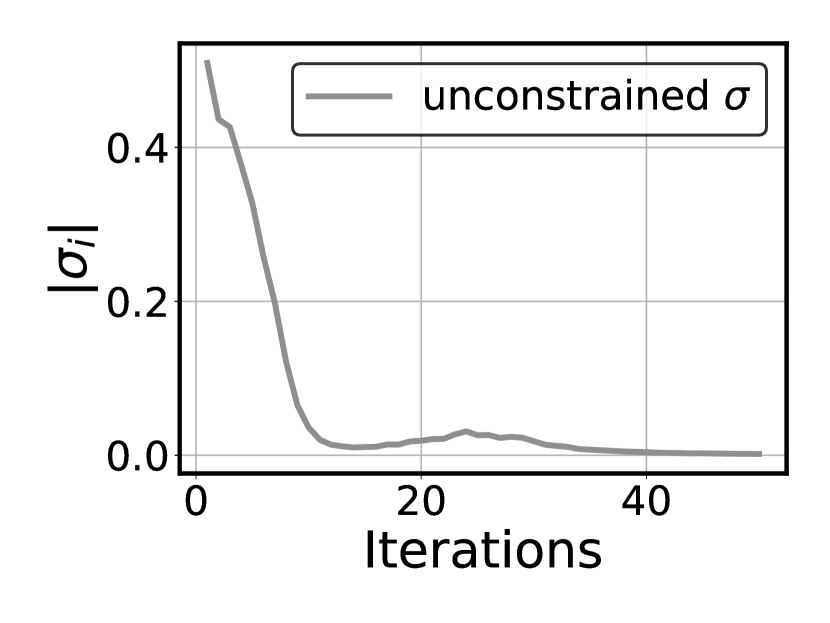
(a) R channel

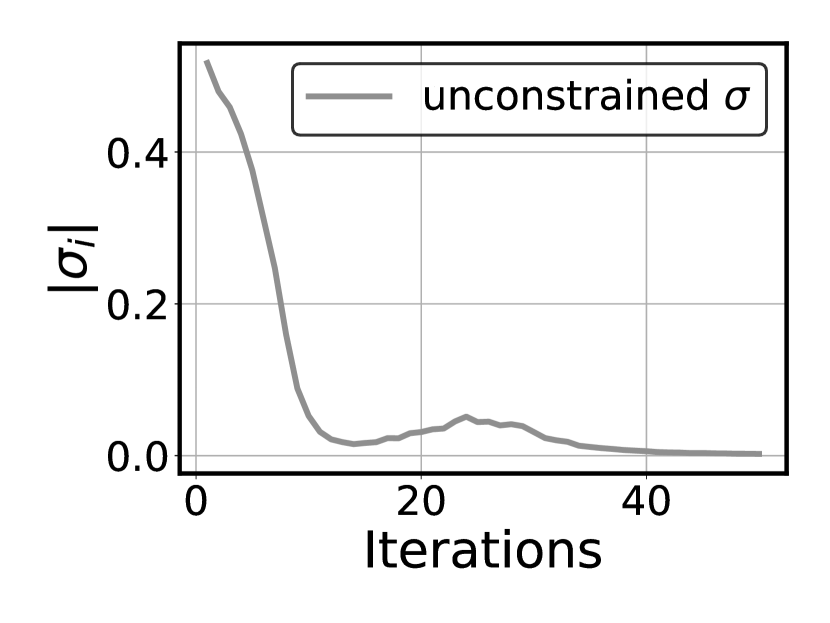
(b) G channel

(c) B channel

Figure 2: The degradation curves of $\bm{\sigma}_{i}$ during training. When $\bm{\sigma}_{i}$ approaching zero, Equation (6) is equivalent to $\ell_{1}$ loss.

Owing to the reparameterization trick [64], learning probabilistic model via Equation (6) seems straightforward. However, there exists a trivial solution to easily bridge the Jensen gap (i.e., $\mathbb{E}[f(\mathbf{z})]=f(\mathbb{E}[\mathbf{z}])$) such that $\bm{\sigma}\in\vec{\mathbf{0}}$. As shown in Figure 2, the output of the $\bm{\sigma}$ branch gradually approaches zero which ultimately eliminates the randomness in our learning target. Similar degradation also occurs in Variational Auto-Encoder (VAE). In a nutshell, VAE is an auto-encoder when latent variable $\mathbf{z}$ that determines encodings distribution lose randomness. VAE regularises its random latent variable $\mathbf{z}$ towards Normal distribution that enables generative process [65]. Otherwise, the latent space will converge to a single point instead of a distribution. That is, VAE degrades into an one-to-one mapping given input images, i.e., an (deterministic) auto-encoder. In light of this, we focus on avoiding the degradation of $\bm{\sigma}$ in the following section.

III-C Beyond $\ell_{1}$ Loss

Data-independent $\bm{\sigma}$ The simplest way is to remove the trainable $\bm{\sigma}$ branch and let $\bm{\sigma}_{i}$ be a small constant $k$ invisible to the human eye. Then, $P(\mathbf{y}|\mathbf{x};\mathbf{W})\sim\mathcal{N}(\bm{\mu};k^{2}\bm{I})$ where $\bm{I}$ refers to an identity matrix. Contracting this term into Equation (6) and rearranging yields:

$$\mathbb{E}_{\mathbf{z}}\Big{[}\|\mathbf{\hat{y}}-(\bm{\mu}+k\cdot\mathbf{z})\|_{1}\Big{]}=\mathbb{E}_{\mathbf{z}}\Big{[}\|\underbrace{\mathbf{(\hat{y}}+\mathbf{z^{\prime}})}_{\mathrm{Noised\ HR}}-\bm{\mu}\|_{1}\Big{]}$$ (9)

where $\mathbf{z^{\prime}}$ is an additive Gaussian noise $\mathcal{N}(0,k)$ and $k\neq 0$. The left hand side of this equation is something we hope to optimize via backward propagation. The right hand side serves is the core of Noise2Noise [53] that restores corrupted images without clean data, i.e., learning super-resolution by only looking at noised HR images.

Though the performance of training on corrupted observations may approach its clean counterpart [53], the noise term can do harm to the optimization process. To be specific, we expect $\bm{\mu}$ to approach $\mathbf{\hat{y}}$ via stochastic gradient descent. However, for some $\mathbf{z^{\prime}}$ satisfying $(\mathbf{(\hat{y}}_{i}-\bm{\mu}_{i})+\mathbf{z^{\prime}})(\mathbf{\hat{y}}_{i}-\bm{\mu}_{i})<0$, we have

$$\mathrm{sgn}(\frac{\partial\|\mathbf{(\hat{y}}+\mathbf{z^{\prime}})-\bm{\mu}\|_{1}}{\partial\bm{\mu}_{i}})=-1\cdot\mathrm{sgn}(\frac{\partial\|\mathbf{\hat{y}}-\bm{\mu}\|_{1}}{\partial\bm{\mu}_{i}})$$

where $\mathbf{z^{\prime}}$ results in gradient ascent instead of descent, which ultimately hinders $\bm{\mu}$ from fitting $\mathbf{\hat{y}}$. To get a good estimate of the proper gradient, it would require sampling massive noised observations given a single clean image, which would be expensive. Hence, we hope to find some $\bm{\sigma}$ that run correct backprop efficiently and retain randomness.

Data-adaptive $\bm{\sigma}$ Fortunately, a delicate $\bm{\sigma}$ gives a definite answer to both. The full equation we want to optimize is:

$$\min_{\bm{\mu}}\ \mathbb{E}_{\mathbf{z}}\Big{[}\big{\|}\mathbf{\hat{y}}-(\bm{\mu}+|\mathbf{\hat{y}}-\bm{\mu}|*\mathbf{z})\big{\|}_{1}\Big{]}$$ (10)

where $|\mathbf{\hat{y}}-\bm{\mu}|$ corresponds to the $\bm{\sigma}$ term and $|\cdot|$ refers to element-wise absolute function. We shall denote Equation (10) as $\ell_{\mathbb{E}}$ in the remaining text for simplicity.

From the view of Equation (9), $\ell_{\mathbb{E}}$ is also in the form of adding some (data-adaptive) noise to HR images. However, for Equation (10), we allow the backprop through $|\mathbf{\hat{y}}-\bm{\mu}|$ instead of regarding it as a scaling factor, which contributes to the following property:

Lemma III.1.

Given a random variable $\mathbf{z}\sim\mathcal{N}(\bm{0},\bm{1})$ and fixed $\mathbf{\hat{y}}$, the gradient direction of $\bm{\mu}$ with respect to the following object

$$\min_{\bm{\mu}}\ \mathbb{E}_{\mathbf{z}}\Big{[}\big{\|}(\bm{\mu}+|\bm{\mu}-\mathbf{\hat{y}}|*\mathbf{z})-\mathbf{\hat{y}}\big{\|}_{1}\Big{]}$$

is always consistent with $\|\bm{\mu}-\mathbf{\hat{y}}\|_{1}$ and $\Big{|}\mathbb{E}_{\mathbf{z}}\big{[}\frac{\partial\ell_{\mathbb{E}}}{\partial\bm{\mu}_{i}}\big{]}\Big{|}$ converges to $1.17$.

Proof.

Since the expectation of random variable $\mathbf{z}$ does not depend on model parameters, we can safely move the gradient symbol into $\mathbb{E}_{\mathbf{z}}[\cdot]$ while maintaning equality:

$$\frac{\partial\ell_{\mathbb{E}}}{\partial\bm{\mu}_{i}}=\mathrm{sgn}\big{(}\bm{\mu}_{i}+|\bm{\mu}_{i}-\mathbf{\hat{y}}_{i}|*\mathbf{z}_{i}-\mathbf{\hat{y}}_{i}\big{)}\big{(}1+\mathbf{z}_{i}*\mathrm{sgn}(\bm{\mu}_{i}-\mathbf{\hat{y}}_{i})\big{)}.$$

Assuming that $\bm{\mu}_{i}>\mathbf{\hat{y}}_{i}$, the above equation can be further simplified as:

$$\frac{\partial\ell_{\mathbb{E}}}{\partial\bm{\mu}_{i}}=\mathrm{sgn}\big{(}(\bm{\mu}_{i}-\mathbf{\hat{y}}_{i})(1+\mathbf{z}_{i})\big{)}\big{(}1+\mathbf{z}_{i}\big{)}.$$

Leaving out the non-differentiable $\mathbf{z}_{i}=-1$, it is easy to prove that

$$\frac{\partial\ell_{\mathbb{E}}}{\partial\bm{\mu}_{i}}=\begin{cases}1+\mathbf{z}_{i},&\forall\mathbf{z}_{i}>-1\\ -1-\mathbf{z}_{i},&\text{otherwise}\end{cases}.$$

In both cases, we always have $\frac{\partial\ell_{\mathbb{E}}}{\partial\bm{\mu}_{i}}>0$. Similarly, for $\bm{\mu}_{i}<\mathbf{\hat{y}}_{i}$, we obtain $\frac{\partial\ell_{\mathbb{E}}}{\partial\bm{\mu}_{i}}<0$ given any $\mathbf{z}_{i}\sim\mathcal{N}(0,1)$. Recall that $\ell_{1}$ norm is not differentiable with respect to the origin. Elsewhere, the partial derivative $\mathrm{sgn}(\bm{\mu}_{i}-\mathbf{\hat{y}}_{i})$ is consistent with the gradient direction of $\frac{\partial\ell_{\mathbb{E}}}{\partial\bm{\mu}_{i}}$ above.

For the estimation of $\Big{|}\mathbb{E}_{\mathbf{z}}\big{[}\frac{\partial\ell_{\mathbb{E}}}{\partial\bm{\mu}_{i}}\big{]}\Big{|}$, we shall begin with $\bm{\mu}_{i}>\mathbf{\hat{y}}_{i}$ to simplify the derivation:

$$\mathbb{E}_{\mathbf{z}}\Big{[}\frac{\partial\ell_{\mathbb{E}}}{\partial\bm{\mu}_{i}}\Big{]} =\int_{-1}^{+\infty}(1+\mathbf{z}_{i})\phi(\mathbf{z}_{i})\mathrm{d}\mathbf{z}_{i}-\int^{-1}_{-\infty}(1+\mathbf{z}_{i})\phi(\mathbf{z}_{i})\mathrm{d}\mathbf{z}_{i}$$

$$=\Phi(+1)-\phi(\mathbf{z}_{i})\big{|}_{-1}^{+\infty}-\Phi(-1)+\phi(\mathbf{z}_{i})\big{|}^{-1}_{-\infty}$$

$$=\Phi(+1)-\Phi(-1)+2\phi(-1)$$

$$\approx 1.16663$$

where $\Phi(\cdot)$ and $\phi(\cdot)$ are the cumulative distribution function (CDF) and probability density function (PDF) of the standard normal distribution respectively. Similarly, we have $\mathbb{E}_{\mathbf{z}}\big{[}\frac{\partial\ell_{\mathbb{E}}}{\partial\bm{\mu}_{i}}\big{]}\approx-1.16663$ for any $\bm{\mu}_{i}<\mathbf{\hat{y}}_{i}$. ∎

For any $\mathbf{z}\sim\mathcal{N}(0,1)$, we have

$$\mathrm{sgn}(\frac{\partial\ell_{\mathbb{E}}}{\partial\bm{\mu}_{i}}) =\mathrm{sgn}(\frac{\partial\|\mathbf{\hat{y}}-\bm{\mu}\|_{1}}{\partial\bm{\mu}_{i}})$$ (11)

$$\Big{|}\mathbb{E}_{\mathbf{z}}\big{[}\frac{\partial\ell_{\mathbb{E}}}{\partial\bm{\mu}_{i}}\big{]}\Big{|} \approx 1.$$ (12)

Note that the gradient direction is always making $\bm{\mu}$ approach $\mathbf{\hat{y}}$ and the step-size converges to nearly one. Therefore, we can safely average the gradient of $\nabla_{\mathbf{W}}\ell_{\mathbb{E}}$ over arbitrarily many samplings of $\mathbf{z}$ and training images $\mathbf{x}$, without the risk of gradient ascent or the problem of vanishing/exploding gradient. Due to the ill-posed nature of super-resolution, $|\mathbf{\hat{y}}-\bm{\mu}|$ can never be a zero vector then the randomness of (10) will be preserved.

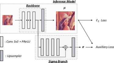
Figure 3: An illustration of the proposed learning scheme and the sigma branch. The newly added branch includes two operations: four Conv+PReLU blocks serve as a mapping function and the upsampler (Pixelshuffle coupled with $3\times 3$ convolution) adjusts the output size. “$\ell_{\mathbb{E}}$” and “Auxiliary Loss” correspond to Equation (10) and Equation (13) respectively. We use $\bm{\mu}$ as the super-resolved image at inference time.

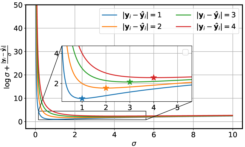
(a) Optimization landscape of $\sigma$.

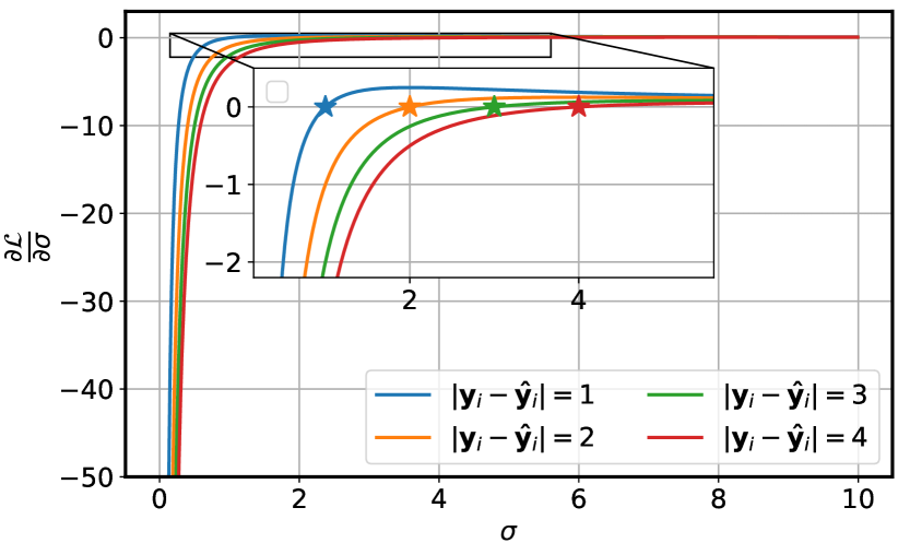
(b) Derivative to $\sigma$.

Figure 4: Objective function and its derivative to $\sigma$ under the naive setting. The star markers indicate the local optimums.

It is shown that $|\mathbf{\hat{y}}-\bm{\mu}|$ plays a core role in learning $\bm{\mu}$ and serves as $\bm{\sigma}$ in $\ell_{\mathbb{E}}$ loss, which inspires us to re-fetch the $\bm{\sigma}$ branch to perform the following multi-task learning except $\ell_{\mathbb{E}}$ loss:

$$\min_{\bm{\sigma}}\ \beta\cdot\big{\|}|\mathbf{\hat{y}}-\bm{\mu}|-\bm{\sigma}\big{\|}_{1}$$ (13)

where $\beta$ is a penalty factor and $\bm{\mu}$ is detached from backward propagation. This equation also, as a by-product, allows us to make a rough estimate of the model uncertainty in SISR via the prediction of $\bm{\sigma}$, e.g., small $\bm{\sigma}_{i}$ means we can be certain of the super-resolved image produced by neural networks, otherwise should be less confident (details in Section IV-G). Finally, Figure 3 further illustrates the overall structure of the proposed scheme.

III-D Revisiting Naive Setting

It is intuitive to directly model the joint probability density function $P(\mathbf{y}_{i},\mathbf{\hat{y}}_{i}|\mathbf{x},\mathbf{W})$ in the form of the PDF of Laplician distribution $\frac{1}{2\bm{\sigma}_{i}}\exp(-\frac{|\mathbf{y}_{i}-\mathbf{\hat{y}}_{i}|}{\bm{\sigma}_{i}})$ without considering $P(\mathbf{\hat{y}}_{i}|\mathbf{y}_{i})$. In this subsection, we argue that this naive setting where $\mathbf{y}_{i}$ and $\bm{\sigma}_{i}$ combine into a unified objective function is not suitable for either image restoration or uncertainty estimation.

Firstly, we are interested in estimating $P(\mathbf{y}_{i},\mathbf{\hat{y}}_{i}|\mathbf{x},\mathbf{W})$ using maximum likelihood estimation

$$\max~{}\log P(\mathbf{y}_{i},\mathbf{\hat{y}}_{i}|\mathbf{x},\mathbf{W}) =\max~{}-\log\bm{\sigma}_{i}-\frac{|\mathbf{y}_{i}-\mathbf{\hat{y}}_{i}|}{\bm{\sigma}_{i}}$$ (14)

$$\Leftrightarrow\min~{}\log\bm{\sigma}_{i}+\frac{|\mathbf{y}_{i}-\mathbf{\hat{y}}_{i}|}{\bm{\sigma}_{i}}$$ (15)

where $\mathbf{y}$ is the predicted SR image. It is easy to prove that Equation (15), as a twice differentiable function of $\bm{\sigma}_{i}$, is convex on an interval $\bm{\sigma}_{i}\in(0,2|\mathbf{y}_{i}-\mathbf{\hat{y}}_{i}|]$. The local optimum is surprisingly

$$\bm{\sigma}^{*}_{i}=|\mathbf{y}_{i}-\mathbf{\hat{y}}_{i}|$$ (16)

which is consistent with the learning target of Equation (13). However, as illustrated in Figure 4, the optimization process can be quite challenging when $|\mathbf{y}_{i}-\mathbf{\hat{y}}_{i}|$ is relatively large due to an ill-behaved (more precisely, flat) loss landscape of $\bm{\sigma}_{i}$. Note that, the averaged $\ell_{1}$ training loss on DIV2K dataset is roughly 3.3 in $2\times$ SR (more than 5 for $3\times$ SR), which implies we could not reach $\bm{\sigma}^{*}_{i}$ since the derivative approaches zero along with $\bm{\sigma}_{i}\rightarrow\bm{\sigma}^{*}_{i}$, as shown in Figure 4(b). In contrast, Equation (13) enjoys a constant derivative almost everywhere with the same $\bm{\sigma}^{*}_{i}$.

Besides, the behavior of Equation (15) can be counter-intuitive when $\bm{\sigma}_{i}\rightarrow\bm{\sigma}^{*}_{i}$, which leads to a weighted MAE loss for the prediction of $\mathbf{y}_{i}$. The gradient then becomes

$$\frac{\partial\mathcal{L}}{\partial\mathbf{y}_{i}}=\frac{1}{\bm{\sigma}_{i}}\text{sgn}(\mathbf{y}_{i}-\mathbf{\hat{y}}_{i})$$ (17)

Assuming that $\bm{\sigma}_{i}\approx\bm{\sigma}^{*}_{i}$, we may rewrite the above equation into

$$\frac{\partial\mathcal{L}}{\partial\mathbf{y}_{i}}\approx\frac{1}{|\mathbf{y}_{i}-\mathbf{\hat{y}}_{i}|}\text{sgn}(\mathbf{y}_{i}-\mathbf{\hat{y}}_{i}).$$ (18)

which indicates that pixels with larger regression error should contribute less to the gradient of $\mathbf{y}$. To be specific, since the magnitude of $\text{sgn}(\mathbf{y}_{i}-\mathbf{\hat{y}}_{i})$ remains $+1$ for all pixels, the gradient will be dominated by $\frac{1}{|\mathbf{y}_{i}-\mathbf{\hat{y}}_{i}|}$. It is common sense that learning based methods should focus on edges with large $|\mathbf{y}_{i}-\mathbf{\hat{y}}_{i}|$ instead of signals in low-frequency with small $|\mathbf{y}_{i}-\mathbf{\hat{y}}_{i}|$. As for Equation (15), it is just the other way around. Therefore, even if $\bm{\sigma}_{i}\rightarrow\bm{\sigma}^{*}_{i}$, one may encounter unexpected results.

IV Experiments

IV-A Dataset

For Bicubic image SR, following the common setting in [9, 38, 66, 15, 11, 12], we conduct all experiments on the 1st-800th images from DIV2K [67] training set then evaluate our models on five benchmarks: Set5 [68], Set14 [69], B100 [70], Urban100 [71] and Manga109 [72] with scale factors $2\times$, $3\times$, $4\times$. To make a fair comparison with early works trained on the tiny dataset [32], we also cite the reproduced DIV2K results [49] in Table IV. For real-world SR, we use the same dataset and training settings proposed in RealSR benchmark [73]. We report PSNR and SSIM on the Y channel in YCbCr space and ignore the same amount of pixels as scales from the border.

Since $\ell_{1}$ loss is also known-to-work for Additive White Gaussian Noise (AWGN) denoising, we evaluate our methods on another representative task: color (Table 4)/grayscale (Table 2) image denoising.

IV-B Training Details

We use low-resolution RGB image patches with the size of $48\times 48$ for training. All HR-LR image pairs are randomly rotated by $90^{\circ}$, $180^{\circ}$, $270^{\circ}$ and flipped horizontally [9]. We set the mini-batch size to 16. Our models are trained by Adam optimizer [74] with $\beta_{1}=0.9$, $\beta_{2}=0.999$, and $\epsilon=10^{-8}$. The initial learning rate is set to $10^{-4}$ and decreases to half at every $2\times 10^{5}$ mini-batch updates. The total training cost is $10^{6}$ iterations [9]. For RealSR, as described in [73], the training patch size is $192\times 192$ and learning rate is fixed at $10^{-4}$. Other details are the same as classical SR. We use the PyTorch framework [75] to implement our methods with an NVIDIA Tesla V100 GPU.

For image denoising, here we use the state-of-the-art DRUNet [76] as a strong baseline method. Following the same settings in [76], we include 400 BSD images [70], 4744 images of Waterloo Exploration Database [77], 900 images from DIV2K [67], and 2750 images from Flick2K dataset [9] as the training dataset. The standard AWGN with noise level $\sigma$ is added to the clean image. A specific noise level is randomly chosen from [0,50] during training. The learning rate starts from $1e^{-4}$ and finally ends at $1.56e^{-6}$. We set the patch size to $192\times 192$ and the batch size is 16 for 4 Nvidia RTX GPUs.

TABLE I: EDSR-baseline [9] results on Set14 ($2\times$) for different learning targets. We use the best setting in the following experiments.

$\ell_{1}$	Eq.(10)	Eq.(13)	PSNR (dB)	SSIM	Training cost
✓			33.57	0.9175	2.00 ms/iter
	✓		33.68	0.9181	2.06 ms/iter
		✓	33.57	0.9176	2.16 ms/iter
✓		✓	33.64	0.9180	2.71 ms/iter
	✓	✓	33.71	0.9185	2.77 ms/iter

TABLE II: Ablation study on the penalty factor $\beta$. (EDSR-baseline [9] on Set14 $2\times$)

$\beta$	0.001	0.005	0.01	0.05	0.1
PSNR (dB)	33.605	33.641	33.707	33.663	33.647
SSIM	0.9176	0.9181	0.9185	0.9184	0.9178

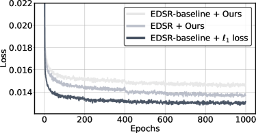
Figure 5: The error curves of training $2\times$ EDSR-baseline (1.37M parameters) and $2\times$ EDSR (42M parameters). Our method enjoys nearly the same convergence speed as $\ell_{1}$ loss. Due to the proposed multi-task learning object, the converged loss value is slightly larger than $\ell_{1}$ loss.

IV-C Ablation Studies

We first present an ablation analysis on each object function in our learning process and report quantitative results in terms of average PSNR and SSIM on Set14 [69] with the scale factor of 2. The baseline results in Table I (i.e., first row) are obtaind using EDSR pre-trained model . In the case of training neural networks by Equation (13) (i.e., third row), we run the backpropagation though both $\bm{\mu}$ and $\bm{\sigma}$ to allow the prediction of super-resolved images via $\bm{\mu}$ branch. The following rows illustrate that both $\ell_{\mathbb{E}}$ loss (Equation (10)) and the multi-task learning (Equation (13)) contribute to higher performances than $\ell_{1}$ baseline. When applying both settings to the original network, we can further improve the PSNR and SSIM results. In the following experiments, we use “Equation (10)+Equation (13)” as the learning target.

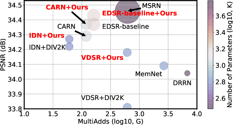
(a) Lightweight Models

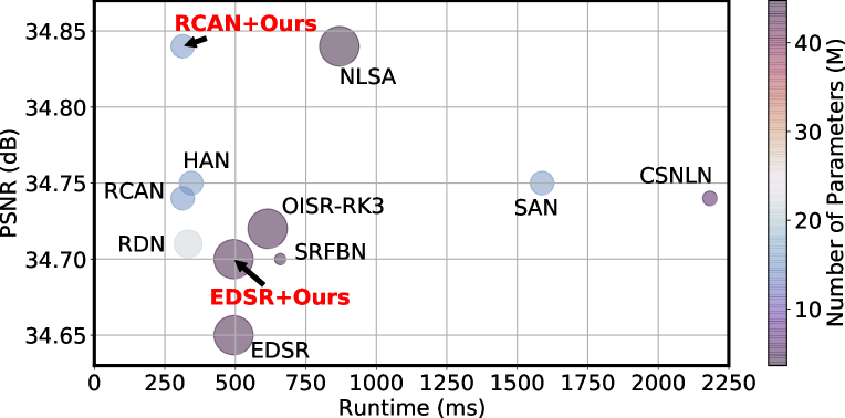
(b) Big Models

Figure 6: Trade-off between the model size and the average PSNR on Set5 [68] (3$\times$). The marker size indicates the number of parameters. The running time is measured on an 720P SR image. (Best viewed in color.)

TABLE III: Quantitative comparison with lightweight models. Our approach improves the performance of early baseline methods to the state-of-the-art. It is shown that networks with simple structures such as EDSR [9] can be competitive with recent elaborate-designed networks. When coupled with efficient models (e.g., CARN [66], IDN [78]), the improvement is consistent as shown in Table IV.

Scale	Methods	#Param.	MAC	Runtime	Set5 [68]		Set14 [69]		B100 [70]		Urban100 [71]
					PSNR	SSIM	PSNR	SSIM	PSNR	SSIM	PSNR	SSIM
2$\times$	VDSR [35]	668K	614.7G	120.8ms	37.53	0.9587	33.03	0.9124	31.90	0.8960	30.76	0.9140
	VDSR+Ours				37.83	0.9600	33.40	0.9158	32.05	0.8983	31.59	0.9226
	EDSR-baseline [9]	1370K	316.2G	56.5ms	37.99	0.9604	33.57	0.9175	32.16	0.8994	31.98	0.9272
	EDSR-baseline+Ours				38.02	0.9606	33.71	0.9185	32.18	0.9001	32.19	0.9292
	CARN [66]	964K	223.4G	56.7ms	37.76	0.9590	33.52	0.9166	32.09	0.8978	31.92	0.9256
	IMDN [79]	694K	159.6G	43.2ms	38.00	0.9605	33.63	0.9177	32.19	0.8996	32.17	0.9283
	OISR [38]	1372K	316.2G	68.8ms	38.02	0.9605	33.62	0.9178	32.20	0.9000	32.21	0.9290
3$\times$	VDSR [35]	668K	614.7G	117.3ms	33.66	0.9213	29.77	0.8314	28.82	0.7976	27.14	0.8279
	VDSR+Ours				34.18	0.9249	30.18	0.8395	28.99	0.8028	27.80	0.8436
	EDSR-baseline [9]	1555K	160.1G	30.4ms	34.37	0.9270	30.28	0.8417	29.09	0.8052	28.15	0.8527
	EDSR-baseline+Ours				34.41	0.9271	30.38	0.8435	29.12	0.8062	28.22	0.8543
	CARN [66]	1149K	118.9G	30.7ms	34.29	0.9255	30.29	0.8407	29.06	0.8034	28.06	0.8493
	IMDN [79]	703K	71.7G	22.4ms	34.36	0.9270	30.32	0.8417	29.09	0.8046	28.17	0.8519
	OISR [38]	1557K	160.1G	36.2ms	34.39	0.9272	30.35	0.8426	29.11	0.8058	28.24	0.8544
4$\times$	VDSR [35]	668K	614.7G	121.4ms	31.35	0.8838	28.01	0.7674	27.29	0.7251	25.18	0.7524
	VDSR+Ours				31.89	0.8900	28.45	0.7778	27.46	0.7327	25.76	0.7734
	EDSR-baseline [9]	1518K	114.2G	21.6ms	32.09	0.8938	28.58	0.7813	27.57	0.7357	26.04	0.7849
	EDSR-baseline+Ours				32.15	0.8933	28.65	0.7831	27.59	0.7377	26.15	0.7885
	CARN [66]	1112K	91.1G	22.5ms	32.13	0.8937	28.60	0.7806	27.58	0.7349	26.07	0.7837
	IMDN [79]	715K	41.1G	11.6ms	32.21	0.8948	28.58	0.7811	27.56	0.7353	26.04	0.7838
	OISR [38]	1520K	114.2G	24.9ms	32.14	0.8947	28.63	0.7819	27.60	0.7369	26.17	0.7888

Table II indicates that a proper $\beta$ matters in the balance between reconstruction loss $\ell_{\mathbb{E}}$ and the auxiliary term. Fortunately, $0.01$ seems to perform well in most cases. For simplicity, we set the channel number of the sigma branch to 160 and introduce a sigmoid function to normalize its output. In our experiments, we notice that nearly half of the estimated $\bm{\sigma}$ approach zero, which correspond to the low-frequency/smooth parts of the high-resolution images (as shown in Figure 9). In light of this, we set $|\mathbf{\hat{y}}_{i}-\bm{\mu}_{i}|$ that is less than the average to zero and focus on the hard samples. Due to the limited computing resource, we did not conduct an ablation study on the structure of the sigma branch, instead simply borrowing the idea of Conv+PReLU proposed in [3], shown in Figure 3.

TABLE IV: PSNR comparison with recently proposed loss functions for SISR. PISR [49] is a Knowledge Distillation framework where a “Teacher” network is required during training. “DIV2K” means models reproduced by [49] using DIV2K dataset with $\ell_{1}$ loss. “EDSR-baseline” refers to the baseline model in [9].

Model	Loss Type	2$\times$ Set5/B100	3$\times$ Set5/B100	4$\times$ Set5/B100
VDSR	$\ell_{2}$	37.53 / 31.90	33.67 / 28.82	31.35 / 27.29
	DIV2K [67]	37.64 / 31.96	33.80 / 28.83	31.37 / 27.25
	Edge [80]	37.70 / 31.98	33.82 / 28.88	31.45 / 27.35
	Riemann [81]	37.72 / 32.04	33.83 / 28.99	31.58 / 27.41
	Teacher [49]	37.77 / 32.00	33.85 / 28.86	31.51 / 27.29
	Ours	37.83 / 32.05	34.18 / 28.99	31.89 / 27.46
IDN	$\ell_{1}$	37.83 / 32.08	34.11 / 28.95	31.82 / 27.41
	DIV2K [67]	37.88 / 32.12	34.22 / 29.02	32.03 / 27.49
	Teacher [49]	37.93 / 32.14	34.31 / 29.03	32.01 / 27.51
	Ours	37.91 / 32.11	34.33 / 29.04	32.09 / 27.53
CARN	$\ell_{1}$	37.76 / 32.09	34.29 / 29.06	32.13 / 27.58
	Teacher [49]	37.82 / 32.08	34.10 / 28.95	31.83 / 27.45
	Ours	37.95 / 32.13	34.37 / 29.08	32.18 / 27.59
EDSR- baseline	$\ell_{1}$	37.99 / 32.16	34.37 / 29.09	32.09 / 27.57
	Riemann [81]	37.87 / 32.14	34.40 / 29.05	32.15 / 27.56
	Ours	38.02 / 32.20	34.43 / 29.11	32.15 / 27.59

TABLE V: Average PSNR (dB) for different models on RealSR testing set. We directly cite SRResNet and RCAN results reported in RealSR benchmark [73]. RCAN used in [73] is smaller than the original model. The running time is measured on a $1200\times 2200$ SR image.

Model	#Param.	Runtime	PSNR(dB)
			2$\times$	3$\times$	4$\times$
Bicubic	–	–	32.61	29.34	27.99
DPS [73]	1.26M	122.8ms	32.71	32.20	28.69
KPN [73]	1.48M	274.8ms	33.86	30.39	28.90
LP-KPN [73]	1.43M	181.3ms	33.90	30.42	28.92
SRResNet [6]	1.31M	143.1ms	33.69	30.18	28.67
SRResNet+Ours			33.87	30.49	28.84
RCAN [10]	8.18M	510.6ms	33.87	30.40	28.88
RCAN+Ours			34.06	30.63	29.00

IV-D Convergence rate

Figure 5 presents a comparison of the convergence rate between EDSR-baseline [9] and standard EDSR model [9], which indicates that deep SR models are still easy to train compared with lightweight counterparts, using the proposed learning object. Besides, the convergence speed of the proposed scheme is similar to $\ell_{1}$ loss, though we introduce randomness during training.

IV-E Quantitative Results

Figure 6 shows the performance comparison of our approach coupled with various SR methods to state-of-the-arts in terms of the number of operations and parameters. We notably improve the Pareto frontier with no extra parameter or computing cost at inference time. When compared with recent learning strategies for image restoration, ours performs the best at most cases (Table IV), even surpasses the knowledge distillation method PISR [49]. Listed SR methods generally benefit from the proposed scheme except for IDN [78] with the scale factor of 2 on B100 [70].

(c) LR

(d) GT

(e) EDSR [9]

(f) [9]+Ours

(g) LR

(h) GT

(i) CARN [66]

(j) [66]+Ours

Figure 7: Visual comparison for $2\times$, $3\times$ and $4\times$ SR with BI models on benchmark datasets.

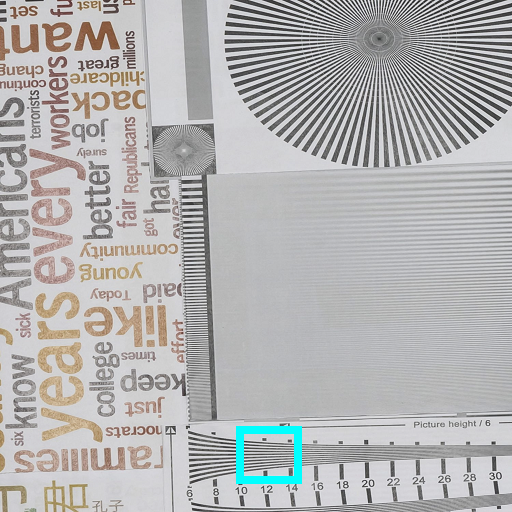
(a) LR

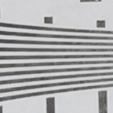
(b) GT

(c) SRRes[6]

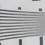
(d) [6]+Ours

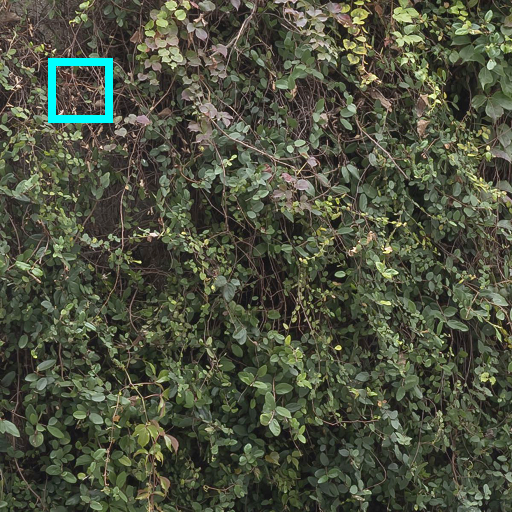
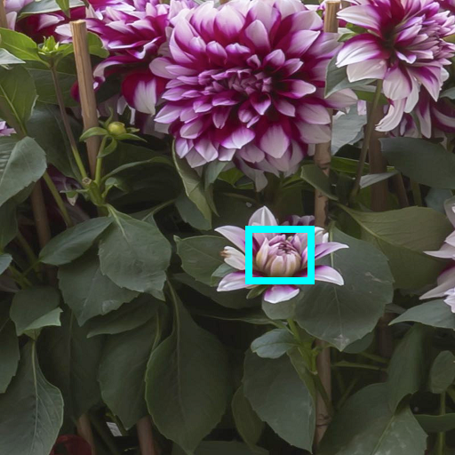
(e) LR

(f) GT

(g) RCAN[10]

(h) [10]+Ours

Figure 8: Qualitative comparison of $3\times$, $4\times$ RealSR results.

TABLE VI: Quantitative comparison with computing-intensive models. We report the multiply-accumulate operations (MAC) and real runtime cost, required to reconstruct a 1280$\times$720 HR image. RCAN [10] coupled with our methods can be competitive with recent leading works.

Scale	Methods	#Param.	Runtime	Set5 [68]		Set14 [69]		B100 [70]		Urban100 [71]		Manga109 [72]
				PSNR	SSIM	PSNR	SSIM	PSNR	SSIM	PSNR	SSIM	PSNR	SSIM
2$\times$	EDSR [9]	40.73M	1003.6ms	38.11	0.9602	33.92	0.9195	32.32	0.9013	32.93	0.9351	39.10	0.9773
	EDSR+Ours			38.24	0.9613	34.05	0.9209	32.36	0.9020	32.96	0.9360	39.19	0.9780
	RCAN [10]	15.44M	667.8ms	38.27	0.9614	34.12	0.9216	32.41	0.9027	33.34	0.9384	39.44	0.9786
	RCAN+Ours			38.25	0.9615	34.16	0.9231	32.40	0.9025	33.19	0.9381	39.41	0.9785
	SAN [11]	15.71M	4817.6ms	38.31	0.9620	34.07	0.9213	32.42	0.9028	33.10	0.9370	39.32	0.9792
	HAN [12]	15.92M	743.3ms	38.27	0.9614	34.16	0.9217	32.41	0.9027	33.35	0.9385	39.46	0.9785
	NLSA [42]	41.80M	1915.8ms	38.34	0.9618	34.08	0.9231	32.43	0.9027	33.42	0.9394	39.59	0.9789
3$\times$	EDSR [9]	43.68M	493.8ms	34.65	0.9280	30.52	0.8462	29.25	0.8093	28.80	0.8653	34.17	0.9476
	EDSR+Ours			34.70	0.9295	30.58	0.8467	29.28	0.8100	28.87	0.8669	34.18	0.9487
	RCAN [10]	15.63M	313.4ms	34.74	0.9299	30.65	0.8482	29.32	0.8111	29.09	0.8702	34.44	0.9499
	RCAN+Ours			34.84	0.9304	30.70	0.8493	29.33	0.8112	29.14	0.8716	34.56	0.9504
	SAN [11]	15.90M	1,587.9ms	34.75	0.9300	30.59	0.8476	29.33	0.8112	28.93	0.8671	34.30	0.9494
	HAN [12]	16.11M	343.7ms	34.75	0.9299	30.67	0.8483	29.32	0.8110	29.10	0.8705	34.48	0.9500
	NLSA [42]	44.75M	869.0ms	34.84	0.9306	30.70	0.8485	29.34	0.8117	29.25	0.8726	34.57	0.9508
4$\times$	EDSR [9]	43.10M	322.6ms	32.46	0.8968	28.80	0.7876	27.71	0.7420	26.64	0.8033	31.02	0.9148
	EDSR+Ours			32.48	0.8985	28.86	0.7883	27.74	0.7423	26.68	0.8045	31.12	0.9165
	RCAN [10]	15.59M	181.1ms	32.63	0.9002	28.87	0.7889	27.77	0.7436	26.82	0.8087	31.22	0.9173
	RCAN+Ours			32.69	0.9005	28.89	0.7892	27.78	0.7437	26.87	0.8094	31.40	0.9185
	SAN [11]	15.86M	880.0ms	32.64	0.9003	28.92	0.7888	27.78	0.7436	26.79	0.8068	31.18	0.9169
	HAN [12]	16.07M	196.8ms	32.64	0.9002	28.90	0.7890	27.80	0.7442	26.85	0.8094	31.42	0.9177
	NLSA [42]	44.15M	523.6ms	32.59	0.9000	28.87	0.7891	27.78	0.7444	26.96	0.8109	31.27	0.9184

We further detail the performance of our approach in contrast to recent lightweight networks [66, 38, 79] in Table III. To well describe different methods, we report the number of parameters, operations required to reconstruct a 720P image, and its average runtime speed measured on an NVIDIA Titan RTX GPU. From Table III, we observe that VDSR [35] trained by the proposed learning process outperforms baselines by a large margin, consistently for all scaling factors. Former state-of-the-art EDSR-baseline [9] with our approach also shows competitive results with recent well-designed lightweight SR methods. We further conduct experiments on the large BI degradation model EDSR [9]. As shown in Table VI, the original model has achieved high PSNR/SSIM on each dataset, while ours can further enhance the performance in most cases. For $3\times$ and $4\times$ Manga109 in particular, the PSNR gains of ours over RCAN are 0.112dB and 0.18 dB.

To further verify the effectiveness of our approach, we conduct extensive experiments on image denoising datasets with a strong baseline method DRUNet [76]. Since DRUNet has achieved promising results, we believe the improvements can be nontrivial. Note that, our methods outperform baseline with $\sim 0.1$dB on Urban100 and consistently bypass the previous leading methods on all datasets. The results are listed in Table 2 and 4.

TABLE VII: Quantitative comparison (average PSNR reported) with state-of-the-art methods for grayscale denoising on benchmark datasets. Best and second best results are shown in red and blue colors, respectively. For DRUNet [76], we use the official well-trained model as a strong baseline . All testing datasets are the same as FFDNet [82].

Dataset	$\sigma$	BM3D [83]	WNNM [84]	DnCNN [85]	IRCNN [86]	FFDNet [82]	N3Net [87]	NLRN [88]	FOCNet [89]	RNAN [90]	MWCNN [91]	GCDN [92]	DRUNet [93]	[93]+Ours
Set12 [85]	15	32.37	32.70	32.86	32.76	32.75	-	33.16	33.07	-	33.15	33.14	33.25	33.29
	25	29.97	30.28	30.44	30.37	30.43	30.55	30.80	30.73	-	30.79	30.78	30.94	30.99
	50	26.72	27.05	27.18	27.12	27.32	27.43	27.64	27.68	27.70	27.74	27.60	27.90	27.95
BSD68 [94]	15	31.08	31.37	31.73	31.63	31.63	-	31.88	31.83	-	31.86	31.83	31.90	31.93
	25	28.57	28.83	29.23	29.15	29.19	29.30	29.41	29.38	-	29.41	29.35	29.46	29.49
	50	25.60	25.87	26.23	26.19	26.29	26.39	26.47	26.50	26.48	26.53	26.38	26.57	26.59
Urban100 [71]	15	32.35	32.97	32.64	32.46	32.40	-	33.45	33.15	-	33.17	33.47	33.44	33.50
	25	29.70	30.39	29.95	29.80	29.90	30.19	30.94	30.64	-	30.66	30.95	31.10	31.17
	50	25.95	26.83	26.26	26.22	26.50	26.82	27.49	27.40	27.65	27.42	27.41	27.96	28.03

TABLE VIII: Quantitative comparison (average PSNR reported) with state-of-the-art methods for color image denoising on benchmark datasets. Best and second best results are shown in red and blue colors, respectively. For DRUNet [76], we use the official well-trained model as a strong baseline . All testing datasets are the same as FFDNet [82].

Dataset	$\sigma$	BM3D [83]	DnCNN [85]	IRCNN [86]	FFDNet [82]	RIDNet [95]	RPCNN [96]	BRDNet [97]	RNAN [98]	RDN [36]	IPT [99]	DRUNet [76]	[76]+Ours
CBSD68 [94]	15	33.52	33.90	33.86	33.87	34.01	-	34.10	-	-	-	34.29	34.33
	25	30.71	31.24	31.16	31.21	31.37	31.24	31.43	-	-	-	31.67	31.72
	50	27.38	27.95	27.86	27.96	28.14	28.06	28.16	28.27	28.31	28.39	28.48	28.53
Kodak24 [100]	15	34.28	34.60	34.69	34.63	-	-	34.88	-	-	-	35.18	35.23
	25	32.15	32.14	32.18	32.13	-	32.34	32.41	-	-	-	32.76	32.81
	50	28.46	28.95	28.93	28.98	-	29.25	29.22	29.58	29.66	29.64	29.71	29.75
McMaster [101]	15	34.06	33.45	34.58	34.66	-	-	35.08	-	-	-	35.39	35.41
	25	31.66	31.52	32.18	32.35	-	32.33	32.75	-	-	-	33.13	33.16
	50	28.51	28.62	28.91	29.18	-	29.33	29.52	29.72	-	29.98	30.07	30.10
Urban100 [71]	15	33.93	32.98	33.78	33.83	-	-	34.42	-	-	-	34.81	34.86
	25	31.36	30.81	31.20	31.40	-	31.81	31.99	-	-	-	32.60	32.67
	50	27.93	27.59	27.70	28.05	-	28.62	28.56	29.08	29.38	29.71	29.60	29.69

TABLE IX: The quality of model uncertainty measured on test datasets. PLL (higher is better $\uparrow$) is the widely accepted uncertainty metric. Since uncertainty should reflect underlying mistakes in super-resolved images, PSNR ($\uparrow$) between the predicted uncertainy $\bm{\sigma}$ and the actual fitting error $|\mathbf{\hat{y}}-\bm{\mu}|$ is also reported (i.e., PSNR between Fig. 9 and Fig. 9).

Model	Scale	S5 [68] PLL/PSNR	S14 [69] PLL/PSNR	B100 [70] PLL/PSNR	U100 [71] PLL/PSNR
EDSR	2$\times$	2.60 / 39.08	1.50 / 35.73	1.08 / 33.70	1.32 / 34.09
	3$\times$	2.28 / 35.82	1.21 / 32.28	0.86 / 30.65	0.74 / 29.98
	4$\times$	2.06 / 33.67	1.12 / 30.44	0.87 / 29.15	0.52 / 27.84
	2$\times$	2.86 / 41.92	2.04 / 37.43	2.25 / 35.86	2.03 / 36.17
	3$\times$	2.43 / 38.27	1.55 / 33.93	1.83 / 32.67	1.31 / 31.81
EDSR +Ours	4$\times$	1.98 / 35.87	1.03 / 31.93	1.49 / 30.95	0.78 / 29.33
CARN	2$\times$	2.58 / 38.56	1.54 / 35.28	1.19 / 33.47	1.14 / 32.96
	3$\times$	2.25 / 35.24	1.28 / 31.94	0.99 / 30.45	0.70 / 29.28
	4$\times$	2.02 / 33.23	1.13 / 30.17	0.91 / 29.01	0.44 / 27.35
	2$\times$	2.80 / 41.67	1.98 / 36.99	2.29 / 35.70	2.07 / 35.35
	3$\times$	2.28 / 37.92	1.40 / 33.62	1.80 / 32.46	1.34 / 31.19
CARN +Ours	4$\times$	2.07 / 35.80	1.17 / 31.89	1.60 / 30.97	0.99 / 29.11

IV-F Qualitative Results

To further illustrate the analysis above, we show visual comparisons in Figure 7 and 8. Bicubic downsampling results in the loss of texture details and structure information, which induces super-resolved images with blurring and artifacts. Even worse, EDSR generates perceptually convincing results such as “barbara” in Set14 (first row in Figure 7). However, the SR image contains several lines with wrong directions. Instead, our models can recover them being more faithful to the ground truth. CARN [66] with ours also obtains much better results by recovering more informative details.

Despite the promising results, networks can make mistakes when exposed to unseen data outside the trained distribution. In this case, we expect information about model uncertainty in addition to the SR images.

IV-G Model Uncertainty

By introducing a posterior distribution $P(\mathbf{y}|\mathbf{x};\mathbf{W})$, we can easily use the predicted $\bm{\sigma}$ as the estimated model uncertainty (Figure 9). Following previous Bayesian models [102, 59, 60, 103], we evaluate uncertainty quality based on the standard metric Predictive Log Likelihood (PLL):

$$\mathrm{PLL}(f(\mathbf{x}),(\mathbf{\hat{y}},\mathbf{x}))=\log P(\mathbf{\hat{y}}|f(\mathbf{x}))$$ (19)

where $P(\mathbf{\hat{y}}|f(\mathbf{x}))$ is the probability of target $\mathbf{\hat{y}}$ generated by a probalistic model $f(\mathbf{x})$. In this paper, $f(\mathbf{x})$ corresponds to the multivariate Gaussian $\mathcal{N}(\bm{\mu},\bm{\sigma}^{2})$ with predicted mean $\bm{\mu}$ and standard deviation $\bm{\sigma}$. $P(\mathbf{\hat{y}}|f(\mathbf{x}))$ is the Gaussian probability density function (PDF) evaluated at $\mathbf{\hat{y}}$.

We report the average PLL of our approach coupled with EDSR [9] and CARN [66] in Table IX. The original EDSR/CARN networks fail to consider the model uncertainty, hence we use their average fitting error $\mathbb{E}_{\mathcal{D}}[|\mathbf{\hat{y}}-\bm{\mu}|]$ calculated on the training dataset $\mathcal{D}$ to create a constant uncertainty estimation, which corresponds to baseline results in Table IX. Any improvement over the baseline reflects a sensible estimate of uncertainty. It is shown that PLL for high upscaling factors are generally low, which indicates that reconstructed $4\times$ image itself can be unreliable, i.e., networks fail to recognize the hidden mistakes.

To improve the interpretability of the model uncertainty, we visualize the predicted $\bm{\sigma}$ in Figure 9. It is shown that the estimated uncertainty strongly correlates with the actual residual error $|\mathbf{\hat{y}}-\bm{\mu}|$. We also report the PSNR results between them to further evaluate the uncertainty quality fairly since PLL has been criticized for being vulnerable to outliers [104].

V Implementation

In this section, we provide Python-style pseudo-codes to facilitate the implementation and further understanding of our approach by automatic differentiation, which has been well supported in mainstream deep-learning frameworks.

As discussed in Section III-B, the main limitation of $\ell_{1}$ loss is the degeneracy problem. By recalling Equation (10)

$$\min_{\bm{\mu}}\ \mathbb{E}_{\mathbf{z}}\Big{[}\big{\|}\mathbf{\hat{y}}-(\bm{\mu}+\underbrace{|\mathbf{\hat{y}}-\bm{\mu}|*\mathbf{z}}_{\text{training variance}})\big{\|}_{1}\Big{]},$$

as $|\mathbf{\hat{y}}-\bm{\mu}|\rightarrow 0$, the variance term approaches zero then the proposed Equation (10) also gradually degrades into $\ell_{1}$ loss

$$\min_{\bm{\mu}}\ \mathbb{E}_{\mathbf{z}}\Big{[}\big{\|}\mathbf{\hat{y}}-(\bm{\mu}+0^{+}*\mathbf{z})\big{\|}_{1}\Big{]}.$$

Note that large models lead to much better results than lightweight models, i.e., the residual error $|\mathbf{\hat{y}}-\bm{\mu}|$ is much smaller in practice, which indicates that cumbersome models may not benefit as much as lightweight ones from Equation (10).

To resolve this issue, we present a simple heuristic method that only applys Equation (10) to “hard samples” with large $|\mathbf{\hat{y}}_{i}-\bm{\mu}_{i}|$. This setting shares a similar idea with Focal-Loss [105] and prevents the vast number of easy samples (i.e., $|\mathbf{\hat{y}}_{i}-\bm{\mu}_{i}|\approx 0$) from overwhelming the sigma branch during training.

Algorithm 1 Pseudo-codes of Equation (10,13) in a Python style.

⬇

# mu: super-resolved images [N, C, H, W]

# hr: high resolution images (ground-truth) [N, C, H, W]

# sigma_pre: predicted standard deviations [N, C, H, W]

sigma_gt = abs(hr - mu) # real residual error

z = randn(hr.shape) # Gaussian random variables (4D tensor)

z = z*(sigma_gt>mean(sigma_gt))

# Set z corresponding to small sigma_gt (i.e., easy samples)

# to zero and focus on the hard samples.

loss_main = mean(abs(mu+sigma_gt*z.detach()-hr)) # Equation (8)

# As in VAE, averaging the gradient over many samples of z

# during training can handle the expectation over z.

loss_aux = mean(abs(sigma_pre-sigma_gt.detach())) # Equation (10)

return loss_main + beta*loss_aux # beta: penalty factor

 *: element-wise product.

(a) LR

(b) HR: $\mathbf{\hat{y}}$

(c) SR: $\bm{\mu}$

(d) $|\mathbf{\hat{y}}-\bm{\mu}|$

(e) $\bm{\sigma}$

Figure 9: The last column (9) visualizes the estimated uncertainty $\bm{\sigma}$ in $3\times$ SR. Dark color indicates large variance, i.e., high uncertainty. Considering the visual differences between HR and SR images and rael residual error (9), $\bm{\sigma}$ depicts a promising uncertainty estimation that approximates the error with high fidelity.

VI Conclusions

In this paper, we present a novel learning process for single image super-resolution with neural networks. Instead of best fitting the ground-truth HR images, we introduce a posterior distribution $P(\mathbf{y}|\mathbf{x};\mathbf{W})$ of underlying natural images $\mathbf{y}$. By sampling from $P(\mathbf{y}|\mathbf{x};\mathbf{W})$, the learning process serves as a multiple-valued mapping that better approximates the local manifold corresponding to the observed HR image. The experiments show that our method can produce SR images with minimal artifacts and the predicted standard deviation of $P(\mathbf{y}|\mathbf{x};\mathbf{W})$, as a by-product, allows us to make meaningful estimations on the model uncertainty.

Though presented in the context of super-resolution, the formulated learning process can be extended to other image reconstruction scenarios with $\mathbf{y}$ following different distributions, not limited to Gaussian. Finally, the performance may be further improved by a more complex sigma branch to predict the actual residual error, which helps to solve both HR image regression and uncertainty estimation simultaneously.

References

- [1] C. Dong, C. C. Loy, K. He, and X. Tang, “Learning a deep convolutional network for image super-resolution,” in Computer Vision - ECCV 2014 - 13th European Conference, Zurich, Switzerland, September 6-12, 2014, Proceedings, Part IV, ser. Lecture Notes in Computer Science, vol. 8692. Springer, 2014, pp. 184–199.
- [2] J. Kim, J. K. Lee, and K. M. Lee, “Deeply-recursive convolutional network for image super-resolution,” in 2016 IEEE Conference on Computer Vision and Pattern Recognition, CVPR 2016, Las Vegas, NV, USA, June 27-30, 2016. IEEE Computer Society, 2016, pp. 1637–1645.
- [3] C. Dong, C. C. Loy, and X. Tang, “Accelerating the super-resolution convolutional neural network,” in Computer Vision - ECCV 2016 - 14th European Conference, Amsterdam, The Netherlands, October 11-14, 2016, Proceedings, Part II, ser. Lecture Notes in Computer Science, vol. 9906. Springer, 2016, pp. 391–407.
- [4] J. Caballero, C. Ledig, A. P. Aitken, A. Acosta, J. Totz, Z. Wang, and W. Shi, “Real-time video super-resolution with spatio-temporal networks and motion compensation,” in 2017 IEEE Conference on Computer Vision and Pattern Recognition, CVPR 2017, Honolulu, HI, USA, July 21-26, 2017. IEEE Computer Society, 2017, pp. 2848–2857.
- [5] Y. Tai, J. Yang, and X. Liu, “Image super-resolution via deep recursive residual network,” in 2017 IEEE Conference on Computer Vision and Pattern Recognition, CVPR 2017, Honolulu, HI, USA, July 21-26, 2017. IEEE Computer Society, 2017, pp. 2790–2798.
- [6] C. Ledig, L. Theis, F. Huszar, J. Caballero, A. Cunningham, A. Acosta, A. P. Aitken, A. Tejani, J. Totz, Z. Wang, and W. Shi, “Photo-realistic single image super-resolution using a generative adversarial network,” in 2017 IEEE Conference on Computer Vision and Pattern Recognition, CVPR 2017, Honolulu, HI, USA, July 21-26, 2017. IEEE Computer Society, 2017, pp. 105–114.
- [7] J. W. Miller, R. M. Goodman, and P. Smyth, “On loss functions which minimize to conditional expected values and posterior proba- bilities,” IEEE Trans. Inf. Theory, vol. 39, no. 4, pp. 1404–1408, 1993.
- [8] H. Zhao, O. Gallo, I. Frosio, and J. Kautz, “Loss functions for image restoration with neural networks,” IEEE Trans. Computational Imaging, vol. 3, no. 1, pp. 47–57, 2017.
- [9] B. Lim, S. Son, H. Kim, S. Nah, and K. M. Lee, “Enhanced deep residual networks for single image super-resolution,” in 2017 IEEE Conference on Computer Vision and Pattern Recognition Workshops, CVPR Workshops 2017, Honolulu, HI, USA, July 21-26, 2017. IEEE Computer Society, 2017, pp. 1132–1140.
- [10] Y. Zhang, K. Li, K. Li, L. Wang, B. Zhong, and Y. Fu, “Image super-resolution using very deep residual channel attention networks,” in Computer Vision - ECCV 2018 - 15th European Conference, Munich, Germany, September 8-14, 2018, Proceedings, Part VII, ser. Lecture Notes in Computer Science, vol. 11211. Springer, 2018, pp. 294–310.
- [11] T. Dai, J. Cai, Y. Zhang, S. Xia, and L. Zhang, “Second-order attention network for single image super-resolution,” in IEEE Conference on Computer Vision and Pattern Recognition, CVPR 2019, Long Beach, CA, USA, June 16-20, 2019. Computer Vision Foundation / IEEE, 2019, pp. 11 065–11 074.
- [12] B. Niu, W. Wen, W. Ren, X. Zhang, L. Yang, S. Wang, K. Zhang, X. Cao, and H. Shen, “Single image super-resolution via a holistic attention network,” in Computer Vision - ECCV 2020 - 16th European Conference, Glasgow, UK, August 23-28, 2020, Proceedings, Part XII, ser. Lecture Notes in Computer Science, vol. 12357. Springer, 2020, pp. 191–207.
- [13] Y. Mei, Y. Fan, Y. Zhou, L. Huang, T. S. Huang, and H. Shi, “Image super-resolution with cross-scale non-local attention and exhaustive self-exemplars mining,” in 2020 IEEE/CVF Conference on Computer Vision and Pattern Recognition, CVPR 2020, Seattle, WA, USA, June 13-19, 2020. IEEE, 2020, pp. 5689–5698.
- [14] J. Liu, W. Zhang, Y. Tang, J. Tang, and G. Wu, “Residual feature aggregation network for image super-resolution,” in 2020 IEEE/CVF Conference on Computer Vision and Pattern Recognition, CVPR 2020, Seattle, WA, USA, June 13-19, 2020. IEEE, 2020, pp. 2356–2365.
- [15] S. Zhou, J. Zhang, W. Zuo, and C. C. Loy, “Cross-scale internal graph neural network for image super-resolution,” in Advances in Neural Information Processing Systems 33: Annual Conference on Neural Information Processing Systems 2020, NeurIPS 2020, December 6-12, 2020, virtual, 2020.
- [16] D. W. Stroock, Probability theory: an analytic view. Cambridge university press, 2010.
- [17] J. P. Allebach and P. W. Wong, “Edge-directed interpolation,” in Proceedings 1996 International Conference on Image Processing, Lausanne, Switzerland, September 16-19, 1996. IEEE Computer Society, 1996, pp. 707–710.
- [18] X. Li and M. T. Orchard, “New edge-directed interpolation,” IEEE Trans. Image Process., vol. 10, no. 10, pp. 1521–1527, 2001.
- [19] L. Zhang and X. Wu, “An edge-guided image interpolation algorithm via directional filtering and data fusion,” IEEE Trans. Image Process., vol. 15, no. 8, pp. 2226–2238, 2006.
- [20] M. Li and T. Q. Nguyen, “Markov random field model-based edge-directed image interpolation,” IEEE Trans. Image Process., vol. 17, no. 7, pp. 1121–1128, 2008.
- [21] J. Sun, Z. Xu, and H. Shum, “Image super-resolution using gradient profile prior,” in 2008 IEEE Computer Society Conference on Computer Vision and Pattern Recognition (CVPR 2008), 24-26 June 2008, Anchorage, Alaska, USA. IEEE Computer Society, 2008.
- [22] Y. Tai, S. Liu, M. S. Brown, and S. Lin, “Super resolution using edge prior and single image detail synthesis,” in The Twenty-Third IEEE Conference on Computer Vision and Pattern Recognition, CVPR 2010, San Francisco, CA, USA, 13-18 June 2010. IEEE Computer Society, 2010, pp. 2400–2407.
- [23] D. Ulyanov, A. Vedaldi, and V. S. Lempitsky, “Deep image prior,” in 2018 IEEE Conference on Computer Vision and Pattern Recognition, CVPR 2018, Salt Lake City, UT, USA, June 18-22, 2018. IEEE Computer Society, 2018, pp. 9446–9454.
- [24] J. Bruna, P. Sprechmann, and Y. LeCun, “Super-resolution with deep convolutional sufficient statistics,” in 4th International Conference on Learning Representations, ICLR 2016, San Juan, Puerto Rico, May 2-4, 2016, Conference Track Proceedings, 2016.
- [25] H. Chang, D. Yeung, and Y. Xiong, “Super-resolution through neighbor embedding,” in 2004 IEEE Computer Society Conference on Computer Vision and Pattern Recognition (CVPR 2004), with CD-ROM, 27 June - 2 July 2004, Washington, DC, USA. IEEE Computer Society, 2004, pp. 275–282.
- [26] X. Gao, K. Zhang, D. Tao, and X. Li, “Image super-resolution with sparse neighbor embedding,” IEEE Trans. Image Process., vol. 21, no. 7, pp. 3194–3205, 2012.
- [27] M. Bevilacqua, A. Roumy, C. Guillemot, and M. Alberi-Morel, “Low-complexity single-image super-resolution based on nonnegative neighbor embedding,” in British Machine Vision Conference, BMVC 2012, Surrey, UK, September 3-7, 2012. BMVA Press, 2012, pp. 1–10.
- [28] G. Freedman and R. Fattal, “Image and video upscaling from local self-examples,” ACM Trans. Graph., vol. 30, no. 2, pp. 12:1–12:11, 2011.
- [29] D. Glasner, S. Bagon, and M. Irani, “Super-resolution from a single image,” in IEEE 12th International Conference on Computer Vision, ICCV 2009, Kyoto, Japan, September 27 - October 4, 2009. IEEE Computer Society, 2009, pp. 349–356.
- [30] Z. Wang, Y. Yang, Z. Wang, S. Chang, J. Yang, and T. S. Huang, “Learning super-resolution jointly from external and internal examples,” IEEE Trans. Image Process., vol. 24, no. 11, pp. 4359–4371, 2015.
- [31] C. Yang and M. Yang, “Fast direct super-resolution by simple functions,” in IEEE International Conference on Computer Vision, ICCV 2013, Sydney, Australia, December 1-8, 2013. IEEE Computer Society, 2013, pp. 561–568.
- [32] R. Timofte, V. D. Smet, and L. V. Gool, “A+: adjusted anchored neighborhood regression for fast super-resolution,” in Computer Vision - ACCV 2014 - 12th Asian Conference on Computer Vision, Singapore, Singapore, November 1-5, 2014, Revised Selected Papers, Part IV, ser. Lecture Notes in Computer Science, vol. 9006. Springer, 2014, pp. 111–126.
- [33] J. Yang, J. Wright, T. S. Huang, and Y. Ma, “Image super-resolution via sparse representation,” IEEE Trans. Image Process., vol. 19, no. 11, pp. 2861–2873, 2010.
- [34] W. Dong, G. Shi, Y. Ma, and X. Li, “Image restoration via simultaneous sparse coding: Where structured sparsity meets gaussian scale mixture,” Int. J. Comput. Vis., vol. 114, no. 2-3, pp. 217–232, 2015.
- [35] J. Kim, J. K. Lee, and K. M. Lee, “Accurate image super-resolution using very deep convolutional networks,” in 2016 IEEE Conference on Computer Vision and Pattern Recognition, CVPR 2016, Las Vegas, NV, USA, June 27-30, 2016. IEEE Computer Society, 2016, pp. 1646–1654.
- [36] Y. Zhang, Y. Tian, Y. Kong, B. Zhong, and Y. Fu, “Residual dense network for image super-resolution,” in 2018 IEEE Conference on Computer Vision and Pattern Recognition, CVPR 2018, Salt Lake City, UT, USA, June 18-22, 2018. IEEE Computer Society, 2018, pp. 2472–2481.
- [37] T. Tong, G. Li, X. Liu, and Q. Gao, “Image super-resolution using dense skip connections,” in IEEE International Conference on Computer Vision, ICCV 2017, Venice, Italy, October 22-29, 2017. IEEE Computer Society, 2017, pp. 4809–4817.
- [38] X. He, Z. Mo, P. Wang, Y. Liu, M. Yang, and J. Cheng, “Ode-inspired network design for single image super-resolution,” in IEEE Conference on Computer Vision and Pattern Recognition, CVPR 2019, Long Beach, CA, USA, June 16-20, 2019. Computer Vision Foundation / IEEE, 2019, pp. 1732–1741.
- [39] X. Mao, C. Shen, and Y. Yang, “Image restoration using very deep convolutional encoder-decoder networks with symmetric skip connections,” in Advances in Neural Information Processing Systems 29: Annual Conference on Neural Information Processing Systems 2016, December 5-10, 2016, Barcelona, Spain, 2016, pp. 2802–2810.
- [40] G. Cheng, A. Matsune, Q. Li, L. Zhu, H. Zang, and S. Zhan, “Encoder-decoder residual network for real super-resolution,” in IEEE Conference on Computer Vision and Pattern Recognition Workshops, CVPR Workshops 2019, Long Beach, CA, USA, June 16-20, 2019. Computer Vision Foundation / IEEE, 2019, pp. 2169–2178.
- [41] P. Liu, H. Zhang, K. Zhang, L. Lin, and W. Zuo, “Multi-level wavelet-cnn for image restoration,” in 2018 IEEE Conference on Computer Vision and Pattern Recognition Workshops, CVPR Workshops 2018, Salt Lake City, UT, USA, June 18-22, 2018. IEEE Computer Society, 2018, pp. 773–782.
- [42] Y. Mei, Y. Fan, and Y. Zhou, “Image super-resolution with non-local sparse attention,” in IEEE Conference on Computer Vision and Pattern Recognition, CVPR 2021, virtual, June 19-25, 2021. Computer Vision Foundation / IEEE, 2021, pp. 3517–3526.
- [43] H. Chen, Y. Wang, T. Guo, C. Xu, Y. Deng, Z. Liu, S. Ma, C. Xu, C. Xu, and W. Gao, “Pre-trained image processing transformer,” CoRR, vol. abs/2012.00364, 2020.
- [44] J. Liang, J. Cao, G. Sun, K. Zhang, L. V. Gool, and R. Timofte, “Swinir: Image restoration using swin transformer,” CoRR, vol. abs/2108.10257, 2021.
- [45] F. Yang, H. Yang, J. Fu, H. Lu, and B. Guo, “Learning texture transformer network for image super-resolution,” in 2020 IEEE/CVF Conference on Computer Vision and Pattern Recognition, CVPR 2020, Seattle, WA, USA, June 13-19, 2020. Computer Vision Foundation / IEEE, 2020, pp. 5790–5799.
- [46] A. Dosovitskiy and T. Brox, “Generating images with perceptual similarity metrics based on deep networks,” in Advances in Neural Information Processing Systems 29: Annual Conference on Neural Information Processing Systems 2016, December 5-10, 2016, Barcelona, Spain, 2016, pp. 658–666.
- [47] J. Johnson, A. Alahi, and L. Fei-Fei, “Perceptual losses for real-time style transfer and super-resolution,” in Computer Vision - ECCV 2016 - 14th European Conference, Amsterdam, The Netherlands, October 11-14, 2016, Proceedings, Part II, ser. Lecture Notes in Computer Science, vol. 9906. Springer, 2016, pp. 694–711.
- [48] M. Mathieu, C. Couprie, and Y. LeCun, “Deep multi-scale video prediction beyond mean square error,” in 4th International Conference on Learning Representations, ICLR 2016, San Juan, Puerto Rico, May 2-4, 2016, Conference Track Proceedings, 2016.
- [49] W. Lee, J. Lee, D. Kim, and B. Ham, “Learning with privileged information for efficient image super-resolution,” in Computer Vision - ECCV 2020 - 16th European Conference, Glasgow, UK, August 23-28, 2020, Proceedings, Part XXIV, ser. Lecture Notes in Computer Science, vol. 12369. Springer, 2020, pp. 465–482.
- [50] Q. Gao, Y. Zhao, G. Li, and T. Tong, “Image super-resolution using knowledge distillation,” in Computer Vision - ACCV 2018 - 14th Asian Conference on Computer Vision, Perth, Australia, December 2-6, 2018, Revised Selected Papers, Part II, ser. Lecture Notes in Computer Science, vol. 11362. Springer, 2018, pp. 527–541.
- [51] E. L. Denton, S. Chintala, A. Szlam, and R. Fergus, “Deep generative image models using a laplacian pyramid of adversarial networks,” in Advances in Neural Information Processing Systems 28: Annual Conference on Neural Information Processing Systems 2015, December 7-12, 2015, Montreal, Quebec, Canada, 2015, pp. 1486–1494.
- [52] X. Yu and F. Porikli, “Ultra-resolving face images by discriminative generative networks,” in Computer Vision - ECCV 2016 - 14th European Conference, Amsterdam, The Netherlands, October 11-14, 2016, Proceedings, Part V, ser. Lecture Notes in Computer Science, vol. 9909. Springer, 2016, pp. 318–333.
- [53] J. Lehtinen, J. Munkberg, J. Hasselgren, S. Laine, T. Karras, M. Aittala, and T. Aila, “Noise2noise: Learning image restoration without clean data,” in Proceedings of the 35th International Conference on Machine Learning, ICML 2018, Stockholmsmässan, Stockholm, Sweden, July 10-15, 2018, ser. Proceedings of Machine Learning Research, vol. 80. PMLR, 2018, pp. 2971–2980.
- [54] J. Batson and L. Royer, “Noise2self: Blind denoising by self-supervision,” in Proceedings of the 36th International Conference on Machine Learning, ICML 2019, 9-15 June 2019, Long Beach, California, USA, ser. Proceedings of Machine Learning Research, vol. 97. PMLR, 2019, pp. 524–533.
- [55] Y. Quan, M. Chen, T. Pang, and H. Ji, “Self2self with dropout: Learning self-supervised denoising from single image,” in 2020 IEEE/CVF Conference on Computer Vision and Pattern Recognition, CVPR 2020, Seattle, WA, USA, June 13-19, 2020. Computer Vision Foundation / IEEE, 2020, pp. 1887–1895.
- [56] L. Yue, H. Shen, J. Li, Q. Yuan, H. Zhang, and L. Zhang, “Image super-resolution: The techniques, applications, and future,” Signal Process., vol. 128, pp. 389–408, 2016.
- [57] Y. Chen, F. Shi, A. G. Christodoulou, Y. Xie, Z. Zhou, and D. Li, “Efficient and accurate MRI super-resolution using a generative adversarial network and 3d multi-level densely connected network,” in Medical Image Computing and Computer Assisted Intervention - MICCAI 2018 - 21st International Conference, Granada, Spain, September 16-20, 2018, Proceedings, Part I, ser. Lecture Notes in Computer Science, vol. 11070. Springer, 2018, pp. 91–99.
- [58] Z. Ghahramani, “Probabilistic machine learning and artificial intelligence,” Nat., vol. 521, no. 7553, pp. 452–459, 2015.
- [59] Y. Gal and Z. Ghahramani, “Dropout as a bayesian approximation: Representing model uncertainty in deep learning,” in Proceedings of the 33nd International Conference on Machine Learning, ICML 2016, New York City, NY, USA, June 19-24, 2016, ser. JMLR Workshop and Conference Proceedings, vol. 48. JMLR.org, 2016, pp. 1050–1059.
- [60] M. Teye, H. Azizpour, and K. Smith, “Bayesian uncertainty estimation for batch normalized deep networks,” in Proceedings of the 35th International Conference on Machine Learning, ICML 2018, Stockholmsmässan, Stockholm, Sweden, July 10-15, 2018, ser. Proceedings of Machine Learning Research, vol. 80. PMLR, 2018, pp. 4914–4923.
- [61] S. Ioffe and C. Szegedy, “Batch normalization: Accelerating deep network training by reducing internal covariate shift,” in Proceedings of the 32nd International Conference on Machine Learning, ICML 2015, Lille, France, 6-11 July 2015, ser. JMLR Workshop and Conference Proceedings, vol. 37. JMLR.org, 2015, pp. 448–456.
- [62] A. Buades, B. Coll, and J. Morel, “A non-local algorithm for image denoising,” in 2005 IEEE Computer Society Conference on Computer Vision and Pattern Recognition (CVPR 2005), 20-26 June 2005, San Diego, CA, USA. IEEE Computer Society, 2005, pp. 60–65.
- [63] ——, “A review of image denoising algorithms, with a new one,” Multiscale Model. Simul., vol. 4, no. 2, pp. 490–530, 2005.
- [64] D. P. Kingma and M. Welling, “Auto-encoding variational bayes,” in 2nd International Conference on Learning Representations, ICLR 2014, Banff, AB, Canada, April 14-16, 2014, Conference Track Proceedings, 2014.
- [65] C. Doersch, “Tutorial on variational autoencoders,” CoRR, vol. abs/1606.05908, 2016.
- [66] N. Ahn, B. Kang, and K. Sohn, “Fast, accurate, and lightweight super-resolution with cascading residual network,” in Computer Vision - ECCV 2018 - 15th European Conference, Munich, Germany, September 8-14, 2018, Proceedings, Part X, ser. Lecture Notes in Computer Science, vol. 11214. Springer, 2018, pp. 256–272.
- [67] E. Agustsson and R. Timofte, “Ntire 2017 challenge on single image super-resolution: Dataset and study,” in The IEEE Conference on Computer Vision and Pattern Recognition (CVPR) Workshops, July 2017.
- [68] M. Bevilacqua, A. Roumy, C. Guillemot, and M. Alberi-Morel, “Low-complexity single-image super-resolution based on nonnegative neighbor embedding,” in British Machine Vision Conference, BMVC 2012, Surrey, UK, September 3-7, 2012. BMVA Press, 2012, pp. 1–10.
- [69] R. Zeyde, M. Elad, and M. Protter, “On single image scale-up using sparse-representations,” in Curves and Surfaces - 7th International Conference, Avignon, France, June 24-30, 2010, Revised Selected Papers, ser. Lecture Notes in Computer Science, vol. 6920. Springer, 2010, pp. 711–730.
- [70] D. R. Martin, C. C. Fowlkes, D. Tal, and J. Malik, “A database of human segmented natural images and its application to evaluating segmentation algorithms and measuring ecological statistics,” in Proceedings of the Eighth International Conference On Computer Vision (ICCV-01), Vancouver, British Columbia, Canada, July 7-14, 2001 - Volume 2. IEEE Computer Society, 2001, pp. 416–425.
- [71] J. Huang, A. Singh, and N. Ahuja, “Single image super-resolution from transformed self-exemplars,” in IEEE Conference on Computer Vision and Pattern Recognition, CVPR 2015, Boston, MA, USA, June 7-12, 2015. IEEE Computer Society, 2015, pp. 5197–5206.
- [72] Y. Matsui, K. Ito, Y. Aramaki, A. Fujimoto, T. Ogawa, T. Yamasaki, and K. Aizawa, “Sketch-based manga retrieval using manga109 dataset,” Multim. Tools Appl., vol. 76, no. 20, pp. 21 811–21 838, 2017.
- [73] J. Cai, H. Zeng, H. Yong, Z. Cao, and L. Zhang, “Toward real-world single image super-resolution: A new benchmark and a new model,” in 2019 IEEE/CVF International Conference on Computer Vision, ICCV 2019, Seoul, Korea (South), October 27 - November 2, 2019. IEEE, 2019, pp. 3086–3095.
- [74] D. P. Kingma and J. Ba, “Adam: A method for stochastic optimization,” in 3rd International Conference on Learning Representations, ICLR 2015, San Diego, CA, USA, May 7-9, 2015, Conference Track Proceedings, 2015.
- [75] A. Paszke, S. Gross, F. Massa, A. Lerer, J. Bradbury, G. Chanan, T. Killeen, Z. Lin, N. Gimelshein, L. Antiga, A. Desmaison, A. Köpf, E. Yang, Z. DeVito, M. Raison, A. Tejani, S. Chilamkurthy, B. Steiner, L. Fang, J. Bai, and S. Chintala, “Pytorch: An imperative style, high-performance deep learning library,” in Advances in Neural Information Processing Systems 32: Annual Conference on Neural Information Processing Systems 2019, NeurIPS 2019, December 8-14, 2019, Vancouver, BC, Canada, 2019, pp. 8024–8035.
- [76] K. Zhang, Y. Li, W. Zuo, L. Zhang, L. Van Gool, and R. Timofte, “Plug-and-play image restoration with deep denoiser prior,” IEEE Transactions on Pattern Analysis and Machine Intelligence, 2021.
- [77] K. Ma, Z. Duanmu, Q. Wu, Z. Wang, H. Yong, H. Li, and L. Zhang, “Waterloo exploration database: New challenges for image quality assessment models,” IEEE Trans. Image Process., vol. 26, no. 2, pp. 1004–1016, 2017.
- [78] Z. Hui, X. Wang, and X. Gao, “Fast and accurate single image super-resolution via information distillation network,” in 2018 IEEE Conference on Computer Vision and Pattern Recognition, CVPR 2018, Salt Lake City, UT, USA, June 18-22, 2018. IEEE Computer Society, 2018, pp. 723–731.
- [79] Z. Hui, X. Gao, Y. Yang, and X. Wang, “Lightweight image super-resolution with information multi-distillation network,” in Proceedings of the 27th ACM International Conference on Multimedia, MM 2019, Nice, France, October 21-25, 2019. ACM, 2019, pp. 2024–2032.
- [80] G. Seif and D. Androutsos, “Edge-based loss function for single image super-resolution,” in 2018 IEEE International Conference on Acoustics, Speech and Signal Processing, ICASSP 2018, Calgary, AB, Canada, April 15-20, 2018. IEEE, 2018, pp. 1468–1472.
- [81] J. Mu, X. Zhang, S. Zhu, and R. Xiong, “Riemannian loss for image restoration,” in IEEE Conference on Computer Vision and Pattern Recognition Workshops, CVPR Workshops 2019, Long Beach, CA, USA, June 16-20, 2019. Computer Vision Foundation / IEEE, 2019, pp. 502–504.
- [82] K. Zhang, W. Zuo, and L. Zhang, “Ffdnet: Toward a fast and flexible solution for cnn-based image denoising,” IEEE Transactions on Image Processing, vol. 27, no. 9, pp. 4608–4622, 2018.
- [83] K. Dabov, A. Foi, V. Katkovnik, and K. Egiazarian, “Image denoising by sparse 3-d transform-domain collaborative filtering,” IEEE Transactions on image processing, vol. 16, no. 8, pp. 2080–2095, 2007.
- [84] S. Gu, L. Zhang, W. Zuo, and X. Feng, “Weighted nuclear norm minimization with application to image denoising,” in IEEE conference on computer vision and pattern recognition, 2014, pp. 2862–2869.
- [85] K. Zhang, W. Zuo, Y. Chen, D. Meng, and L. Zhang, “Beyond a gaussian denoiser: Residual learning of deep cnn for image denoising,” IEEE transactions on image processing, vol. 26, no. 7, pp. 3142–3155, 2017.
- [86] K. Zhang, W. Zuo, S. Gu, and L. Zhang, “Learning deep cnn denoiser prior for image restoration,” in IEEE Conference on Computer Vision and Pattern Recognition, 2017, pp. 3929–3938.
- [87] T. Plötz and S. Roth, “Neural nearest neighbors networks,” arXiv preprint arXiv:1810.12575, 2018.
- [88] D. Liu, B. Wen, Y. Fan, C. C. Loy, and T. S. Huang, “Non-local recurrent network for image restoration,” arXiv preprint arXiv:1806.02919, 2018.
- [89] X. Jia, S. Liu, X. Feng, and L. Zhang, “Focnet: A fractional optimal control network for image denoising,” in IEEE Conference on Computer Vision and Pattern Recognition, 2019, pp. 6054–6063.
- [90] Y. Zhang, K. Li, K. Li, B. Zhong, and Y. Fu, “Residual non-local attention networks for image restoration,” arXiv preprint arXiv:1903.10082, 2019.
- [91] P. Liu, H. Zhang, K. Zhang, L. Lin, and W. Zuo, “Multi-level wavelet-cnn for image restoration,” in IEEE conference on computer vision and pattern recognition workshops, 2018, pp. 773–782.
- [92] D. Valsesia, G. Fracastoro, and E. Magli, “Deep graph-convolutional image denoising,” IEEE Trans. Image Process., vol. 29, pp. 8226–8237, 2020.
- [93] K. Zhang, Y. Li, W. Zuo, L. Zhang, L. Van Gool, and R. Timofte, “Plug-and-play image restoration with deep denoiser prior,” IEEE Transactions on Pattern Analysis and Machine Intelligence, 2021.
- [94] D. Martin, C. Fowlkes, D. Tal, and J. Malik, “A database of human segmented natural images and its application to evaluating segmentation algorithms and measuring ecological statistics,” in IEEE International Conference on Computer Vision, 2001, pp. 416–423.
- [95] S. Anwar and N. Barnes, “Real image denoising with feature attention,” in 2019 IEEE/CVF International Conference on Computer Vision, ICCV 2019, Seoul, Korea (South), October 27 - November 2, 2019. IEEE, 2019, pp. 3155–3164.
- [96] Z. Xia and A. Chakrabarti, “Identifying recurring patterns with deep neural networks for natural image denoising,” in IEEE Winter Conference on Applications of Computer Vision, 2020, pp. 2426–2434.
- [97] C. Tian, Y. Xu, and W. Zuo, “Image denoising using deep cnn with batch renormalization,” Neural Networks, vol. 121, pp. 461–473, 2020.
- [98] Y. Zhang, K. Li, K. Li, B. Zhong, and Y. Fu, “Residual non-local attention networks for image restoration,” in 7th International Conference on Learning Representations, ICLR 2019, New Orleans, LA, USA, May 6-9, 2019. OpenReview.net, 2019.
- [99] H. Chen, Y. Wang, T. Guo, C. Xu, Y. Deng, Z. Liu, S. Ma, C. Xu, C. Xu, and W. Gao, “Pre-trained image processing transformer,” in IEEE Conference on Computer Vision and Pattern Recognition, 2021, pp. 12 299–12 310.
- [100] R. Franzen, “Kodak lossless true color image suite,” source: http://r0k. us/graphics/kodak, vol. 4, no. 2, 1999.
- [101] L. Zhang, X. Wu, A. Buades, and X. Li, “Color demosaicking by local directional interpolation and nonlocal adaptive thresholding,” Journal of Electronic imaging, vol. 20, no. 2, p. 023016, 2011.
- [102] J. M. Hernández-Lobato and R. P. Adams, “Probabilistic backpropagation for scalable learning of bayesian neural networks,” in Proceedings of the 32nd International Conference on Machine Learning, ICML 2015, Lille, France, 6-11 July 2015, ser. JMLR Workshop and Conference Proceedings, vol. 37. JMLR.org, 2015, pp. 1861–1869.
- [103] T. D. Bui, D. Hernández-Lobato, J. M. Hernández-Lobato, Y. Li, and R. E. Turner, “Deep gaussian processes for regression using approximate expectation propagation,” in Proceedings of the 33nd International Conference on Machine Learning, ICML 2016, New York City, NY, USA, June 19-24, 2016, ser. JMLR Workshop and Conference Proceedings, vol. 48. JMLR.org, 2016, pp. 1472–1481.
- [104] R. Selten, “Axiomatic characterization of the quadratic scoring rule,” Experimental Economics, vol. 1, no. 1, pp. 43–61, 1998.
- [105] T. Lin, P. Goyal, R. B. Girshick, K. He, and P. Dollár, “Focal loss for dense object detection,” in IEEE International Conference on Computer Vision, ICCV 2017, Venice, Italy, October 22-29, 2017. IEEE Computer Society, 2017, pp. 2999–3007.