Spatial meshing for general
Bayesian multivariate models

Abstract

Quantifying spatial and/or temporal associations in multivariate geolocated data of different types is achievable via spatial random effects in a Bayesian hierarchical model, but severe computational bottlenecks arise when spatial dependence is encoded as a latent Gaussian process (GP) in the increasingly common large scale data settings on which we focus. The scenario worsens in non-Gaussian models because the reduced analytical tractability leads to additional hurdles to computational efficiency. In this article, we introduce Bayesian models of spatially referenced data in which the likelihood or the latent process (or both) are not Gaussian. First, we exploit the advantages of spatial processes built via directed acyclic graphs, in which case the spatial nodes enter the Bayesian hierarchy and lead to posterior sampling via routine Markov chain Monte Carlo (MCMC) methods. Second, motivated by the possible inefficiencies of popular gradient-based sampling approaches in the multivariate contexts on which we focus, we introduce the simplified manifold preconditioner adaptation (SiMPA) algorithm which uses second order information about the target but avoids expensive matrix operations. We demostrate the performance and efficiency improvements of our methods relative to alternatives in extensive synthetic and real world remote sensing and community ecology applications with large scale data at up to hundreds of thousands of spatial locations and up to tens of outcomes. Software for the proposed methods is part of R package meshed, available on CRAN.

Keywords: multivariate spatial models, directed acyclic graphs, domain partitioning, latent Gaussian processes.

1 Introduction

Geolocated data are routinely collected in many fields and motivate the development of geostatistical models based on Gaussian processes (GPs). GPs are appealing due to their analytical tractability, their flexibility via a multitude of covariance or kernel choices, and their ability to effectively represent and quantify uncertainty. When Gaussian distributional assumptions are appropriate, GPs may be used directly as correlation models for the multivariate response. Otherwise, flexible models of multivariate spatial association can in principle be built via assumptions of conditional independence of the outcomes on a latent GP encoding space- and/or time-variability, regardless of data type. The poor scalability of naïve implementations of GPs to large scale data is addressed in a growing body of literature. Sun et al., (2011), Banerjee, (2017) and Heaton et al., (2019) review and compare methods for big data geostatistics. Methods include low-rank approaches (Banerjee et al., , 2008; Cressie and Johannesson, , 2008), covariance tapering (Furrer et al., , 2006; Kaufman et al., , 2008), domain partitioning (Sang and Huang, , 2012; Stein, , 2014), local approximations (Gramacy and Apley, , 2015), and composite likelihood approximations (Stein et al., , 2004). In particular, a popular strategy is to assume sparsity in the Gaussian precision matrix via Gaussian random Markov fields (GRMF; Rue and Held, , 2005) which can be represented as sparse undirected graphical models. Proper joint densities are a result of using directed acyclic graphs (DAG), leading to Vecchia’s approximation (Vecchia, , 1988), nearest-neighbor GPs (NNGPs; Datta et al., 2016a, ), and generalizations (see e.g. Katzfuss, , 2017; Katzfuss and Guinness, , 2021). DAGs can be designed by taking a small number of “past” neighbors after choosing an arbitrary ordering of the data. In models of the response and in the conditionally-conjugate latent Gaussian case, posterior computations rely on sparse-matrix routines for scalability (Finley et al., , 2019; Jurek and Katzfuss, , 2020), enabling fast cross-validation (Shirota et al., , 2019; Banerjee, , 2020). Alternatives to sparse-matrix algorithms involve Gibbs samplers whose efficiency improves by prespecifying a DAG defined on domain partitions, resulting in spatially meshed GPs (MGPs; Peruzzi et al., , 2020). These perspectives are reinforced when considering multivariate outcomes (see e.g. Zhang and Banerjee, 2021; Dey et al., 2021; Peruzzi and Dunson, 2021).

The literature on scalable GPs predominantly relies on Gaussian assumptions on the outcomes, but in many applied contexts these assumptions are restrictive, inflexible, or inappropriate. For example, vegetation phenologists may wish to characterize the life cycle of plants in mountainous regions using remotely sensed Leaf Area Index (LAI, a count variable) and relate it to snow cover during 8 day periods (SC, a discrete variable whose values range from 0 to 8—see e.g., Figure 1). Similarly, community ecologists are faced with spatial patterns when considering dichotomous presence/absence data of several animal species (Figure 2). In this article, we address this key gap in the literature, which is how to construct arbitrary Bayesian multivariate geostatistical models which (1) may include non-Gaussian components, (2) lead to efficient computation for massive datasets.

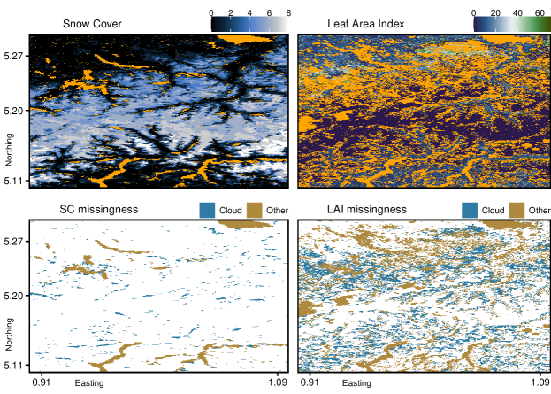
Figure 1: Snow cover (left) and Leaf Area Index, as measured by the MODIS-TERRA satellite. Missing data are in orange. Bottom maps detail the extents of cloud cover and other phenomena negatively impacting data quality.

There are considerable challenges in these contexts for efficient Bayesian computation when avoiding Gaussian distributional assumptions on the outcomes. General purpose Markov chain Monte Carlo (MCMC) methods can in principle be used to draw samples from the posterior distribution of the latent process by making local proposals within accept/reject schemes. However, due to the huge dimensionality of the parameter space, poor mixing and slow convergence are likely. For instance, random-walk Metropolis proposals are cheaply computed but lack in efficiency as they overlook the local geometry of the high dimensional posterior. Alternatively, one may consider gradient-based MCMC methods such as the Metropolis-adjusted Langevin algorithm (MALA; Roberts and Stramer, 2002), Hamiltonian Monte Carlo (HMC; Duane et al., 1987; Neal, 2011; Betancourt, 2018) and others such as MALA and HMC on the Riemannian manifold (Girolami and Calderhead, , 2011) or the no-U-turn sampler (NUTS; Hoffman and Gelman, , 2014) used in the Stan probabilistic programming language (Carpenter et al., , 2017). These methods are appealing because they modulate proposal step sizes using local gradient and/or higher order information of the target density. Unfortunately, their performance very rapidly drops with parameter dimension (Dunson and Johndrow, , 2020). Although it is common in other contexts to rely on subsamples to cheaply approximate gradients, Johndrow et al., (2020) show that such approximate MCMC algorithms are either slow or have large approximation error.

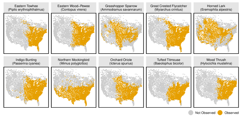
Figure 2: An extract of dichotomized North American Breeding Bird Survey data. Orange points correspond to locations at which at least 1 individual has been observed.

Such issues can be tackled by considering low-rank models, which facilitate the design of more efficient proposals as they involve parameters of greatly reduced dimension. Certain low-rank models endowed with conjugate full conditional distributions (Bradley et al., , 2018, 2019) lead to always-accepted Gibbs proposals. However, excessive dimension reduction—which may be necessary for acceptable MCMC performance—may lead to oversmoothing of the spatial surface, overlooking the small-range variability that frequently occurs in big spatial data (Banerjee et al., , 2010). Alternative dimension reduction strategies via divide-and-conquer methods that combine posterior samples obtained via MCMC from data subsets typically rely on assumptions of independence that are inappropriate in the highly correlated data settings in which we are interested (Neiswanger et al., , 2014; Wang and Dunson, , 2014; Wang et al., 2015b, ; Nemeth and Sherlock, , 2018; Blomstedt et al., , 2019; Mesquita et al., , 2020) or have only considered univariate Gaussian likelihoods (Guhaniyogi and Banerjee, , 2018).

The poor practical performance of MCMC in high dimensional settings has motivated the development of MCMC-free methods for posterior computation that take advantage of Laplace approximations (Sengupta and Cressie, , 2013; Zilber and Katzfuss, , 2020). In particular, the integrated nested Laplace approximation (INLA; Rue et al., , 2009) iterates between Gaussian approximations of the conditional posterior of the latent effects, and numerical integrations over the hyperparameters. INLAs are accurate because of the non-negligible impact the Gaussian prior on the latent process has on its posterior; they achieve scalability to big spatial data by forcing sparsity on the Gaussian precision matrix via a GMRF assumption (Lindgren et al., , 2011). INLAs are reliable alternatives to MCMC methods in several settings, but may be outperformed by carefully-designed MCMC methods in terms of accuracy or uncertainty quantification (Taylor and Diggle, , 2014). Furthermore, the practical reliance of INLAs on Matérn covariance models with small dimensional hyperparameters for fast numerical integration makes them less flexible than MCMC methods in multivariate contexts or whenever special-purpose parametric covariance functions are required.

In this article, we introduce methodological and computational innovations for scalable posterior computations for general non-Gaussian spatial models. Our contributions include a class of Bayesian hierarchical models of multivariate outcomes of possibly different types based on spatial meshing of a latent multivariate process. In our treatment, outcomes can be misaligned—i.e., not all measured at all spatial locations—and relatively large in number, and there is no Gaussian assumption on the latent process. We maintain this perspective when developing posterior sampling methods. In particular, we develop a new Langevin algorithm which, based on ideas related to manifold MALA, adaptively builds a preconditioner but also avoids cubic-cost operations, leading to efficiency improvements in the contexts in which we focus. Our methods enable computations on data of size $10^{5}$ or more. Unlike low-rank methods, we do not require restrictive dimensionality reduction at the level of the latent process. Unlike INLA, our computational methods are exact (upon convergence) for a class of valid spatial processes which is not restricted to latent GPs with Matérn covariances; furthermore, our methods are hit by a smaller computational penalty in higher-dimensional multivariate settings. Our methods are generally applicable to models of spatially referenced data, but we highlight the connections between Langevin methods and the Gibbs sampler available for Gaussian outcomes, and we develop new results for latent coregionalization models using MGPs. In applications, we consider Student-t processes, NUTS, and other cross-covariance models as methodological and computational alternatives to latent GPs, Langevin algorithms, and coregionalization models, respectively. Software for the proposed methods and the related posterior sampling algorithms is available as part of the meshed package for R, available on CRAN.

The article proceeds as follows. Section 2 outlines our model for spatially-referenced multivariate outcomes of different types and introduces general purpose methods and algorithms for scaling computations to high dimensional spatial data. Section 3 outlines Langevin methods for posterior sampling of the latent process and introduces a novel algorithm for multivariate spatial models. Section 4 translates the proposed methodologies for the latent Gaussian model of coregionalization. The remaining sections highlight algorithmic efficiency in applications on large synthetic and real world datasets motivated by remote sensing and spatial community ecology. The supplementary material includes alternative constructions of our proposed methods based on latent grids, Student-t processes, and NUTS for posterior computations, in addition to proofs, practical guidelines, and additional simulations.

2 Meshed Bayesian multivariate models for non-Gaussian data

We introduce our model for multivariate outcomes of possibly different types (e.g. continuous and counts) which also allows for misalignment. Let ${\cal G}=\{\boldsymbol{A},\boldsymbol{E}\}$ be a DAG with nodes $\boldsymbol{A}=\{a_{1},\dots,a_{M}\}$ and edges $\boldsymbol{E}=\{\text{Par}(a):a\in\boldsymbol{A}\}$, where $\text{Par}(a)\subset A$ is referred to as the parent set of $a$. Let ${\cal D}$ be the input domain and ${\cal S}\subset{\cal D}$ denote a user-specified set of “knots” or “reference locations.” We partition ${\cal S}$ into subsets ${\cal S}_{i}\subset{\cal S}$ such that ${\cal S}_{i}\cap{\cal S}_{j}=\emptyset$ if $i\neq j$ and $\cup_{i=1}^{M}{\cal S}_{i}={\cal S}$. Then, we setup our hierarchical model for multivariate outcomes as:

$$y_{j}(\boldsymbol{\ell})\,|\,\eta_{j}(\boldsymbol{\ell}),\gamma_{j}\sim F_{j}(\eta_{j}(\boldsymbol{\ell}),\gamma_{j}), \qquad\eta_{j}(\boldsymbol{\ell})=\boldsymbol{x}_{j}(\boldsymbol{\ell})^{\top}\bbeta_{j}+w_{j}(\boldsymbol{\ell}),$$ (1)

$$\bbeta_{j},\gamma_{j}\sim\pi(\bbeta_{j},\gamma_{j}) \boldsymbol{\theta}\sim\pi(\boldsymbol{\theta}),\quad\boldsymbol{w}(\cdot)\sim\Pi_{{\cal G}}$$

where $F_{j}$ is the probability distribution of the $j$th outcome, parametrized by an unknown constant $\gamma_{j}$ and the spatially-referenced term $\eta_{j}(\boldsymbol{\ell})$. The linear term $\eta_{j}(\boldsymbol{\ell})$ includes a $p_{j}$-dimensional vector of covariates specific for the $j$th outcome, denoted by $\boldsymbol{x}_{j}(\boldsymbol{\ell})$, whereas $w_{j}(\boldsymbol{\ell})$ is the $j$th element of the random vector $\boldsymbol{w}(\boldsymbol{\ell})$, for $j=1,\dots,q$. Given a set of locations ${\cal L}\subset{\cal D}$ of size $n_{{\cal L}}$ we denote $\boldsymbol{w}_{{\cal L}}=(\boldsymbol{w}(\boldsymbol{\ell}_{1})^{\top},\boldsymbol{w}(\boldsymbol{\ell}_{2})^{\top},\ldots,\boldsymbol{w}(\boldsymbol{\ell}_{n_{{\cal L}}})^{\top})^{\top}$. We assume $\boldsymbol{w}_{{\cal L}}$ is the finite realization at ${\cal L}$ of an infinite-dimensional latent process $\boldsymbol{w}(\cdot)$, with law $\Pi_{{\cal G}}$ and density $\pi_{{\cal G}}$, which characterizes spatial/temporal dependence between outcomes. We construct such a process by enforcing conditional independence assumptions encoded in ${\cal G}$ onto the law $\Pi$ of a $q$-variate spatial process (also referred to as the base or parent process). For locations $\boldsymbol{\ell}\in{\cal S}$, we make the assumption that $\pi_{{\cal G}}$ factorizes according to ${\cal G}$. This means $\pi_{{\cal G}}(\boldsymbol{w}_{\cal S}\,|\,\boldsymbol{\theta})=\prod_{a_{i}\in\boldsymbol{A}}\pi(\boldsymbol{w}_{i}\,|\,\boldsymbol{w}_{[i]},\boldsymbol{\theta})$, where we denote $\boldsymbol{w}_{i}=\boldsymbol{w}_{{\cal S}_{i}}$ and $\boldsymbol{w}_{[i]}$ is the vector of $\boldsymbol{w}(\cdot)$ at locations $\boldsymbol{\ell}\in\cup_{a_{j}\in\text{Par}(a_{i})}S_{j}$ – i.e. the set of locations mapped to parents of $a_{i}$. For locations $\boldsymbol{\ell}\in{\cal U}={\cal D}\setminus{\cal S}$, we assume conditional independence given a set of parents $[\boldsymbol{\ell}]\subset\boldsymbol{A}$, which means $\pi_{{\cal G}}(\boldsymbol{w}_{{\cal U}}\mid\boldsymbol{w}_{{\cal S}},\boldsymbol{\theta})=\prod_{\boldsymbol{\ell}\in{\cal U}}\pi(\boldsymbol{w}(\boldsymbol{\ell})\mid\boldsymbol{w}_{[\boldsymbol{\ell}]},\boldsymbol{\theta})$ where $\boldsymbol{w}_{[\boldsymbol{\ell}]}$ is a vector collecting realizations of $\boldsymbol{w}(\cdot)$ at locations ${\cal S}_{[\boldsymbol{\ell}]}=\cup_{\boldsymbol{a}_{i}\in[\boldsymbol{\ell}]}{\cal S}_{i}$.

2.1 DAG and partition choice

We refer to the method of building spatial processes via sparse DAGs associated to domain partitioning as spatial meshing. Several options for constructing ${\cal G}$ and populating and partitioning ${\cal S}$ are available, but sparsity assumptions on ${\cal G}$ are necessary to avoid computational bottlenecks in using $\Pi_{{\cal G}}$. Specifically, we restrict our focus on sparse DAGs such that $|\texttt{mb}(a)|\leq m$ for all $a\in\boldsymbol{A}$, where $\texttt{mb}(a)$ is the Markov blanket of $a$, and $m$ is a small number. The Markov blanket of a node in a DAG is the set $\texttt{mb}(a)=\text{Par}(a)\cup\text{Chi}(a)\cup\text{Copar}(a)$ which enumerates the parents of $a$ along with the set of children of $a$, $\text{Chi}(a)=\{b\in\boldsymbol{A}:a\in\text{Par}(b)\}$, and the set of co-parents of $a$, $\text{Copar}(a)=\{c\in\boldsymbol{A}:c\neq a\text{ and }\{a,c\}\subset\text{Par}(b)\text{ for some }b\in\text{Chi}(a)\}$—this is the set of $a$’s children’s other parents. We additionally assume that the undirected moral graph $\bar{{\cal G}}$ obtained by adding pairwise edges between co-parents has a small number of colors; if node $a$ has color $c$, then no elements of $\texttt{mb}(a)$ have the same color.

Figure 3: Directed acyclic graph representing a special case of model (1). For simplicity, we omit the directed edges from $(\bbeta_{j},\gamma_{j})$ to each $y_{j}(\boldsymbol{\ell})$, $\boldsymbol{\ell}\in{\cal T}$. If $y_{j}(\boldsymbol{\ell})$ is unobserved and therefore $\boldsymbol{\ell}\notin{\cal T}_{j}$, the corresponding node is missing.

Figure 3 visualizes (1) when implemented on a “cubic” spatial DAG using row-column indexing of the nodes resulting in $M=M_{\text{row}}\cdot M_{\text{col}}$ and ${\cal S}=\cup_{i=1}^{M_{\text{row}}}\cup_{j=1}^{M_{\text{col}}}S_{ji}$. Even though DAGs are abstract representations of conditional independence assumptions, nodes of the DAG in Figure 3 conform to a single pattern (i.e., edges from left and bottom nodes, and to right and top nodes). As a consequence, the moral graph $\bar{{\cal G}}$ only adds undirected edges between $a_{i+1,j}$ and $a_{i,j+1}$ for all $i=1,\dots,M_{\text{row}}-1$ and $j=1,\dots,M_{\text{col}}-1$ and has 4 colors (for node $a_{ij}$, we assign one of four color labels $\{ee,eo,oe,oo\}$ depending on whether $i$ and $j$ are even or odd, e.g. $\text{Color}(a_{32})=oe$). We refer to this kind of DAG as a cubic DAG as it naturally extends to a hypercube structure in $d>2$ dimensions.

Once a sparse DAG has been set, one needs to associate each node to a partition ${\cal S}_{i}$ of ${\cal S}$. With cubic DAGs, the $i$th node of ${\cal G}$ can be associated to the $i$th domain partition found via axis-parallel tiling, or via Voronoi tessellations using a grid of centroids. These two partitioning strategies are equivalent when data have no gaps; otherwise, the latter strategy simplifies the proposal in Peruzzi et al., (2020) and can be used to guarantee that every domain partition includes observations, see e.g. Figure 4.

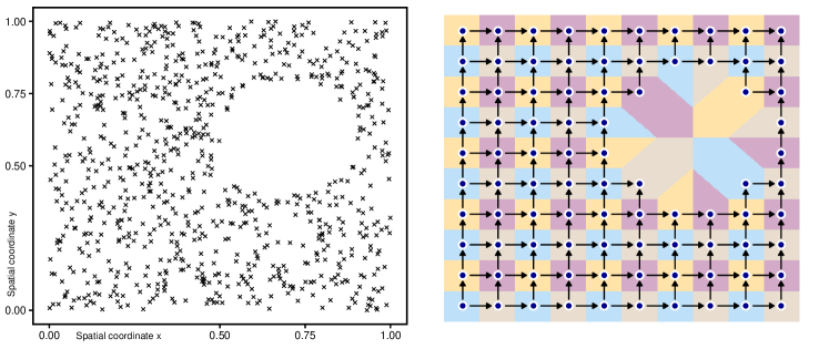
Figure 4: Visualizing cubic DAG and associated domain partitioning. Left: scatter of ${\cal S}$ locations. Right: ${\cal G}$ overlaid to partitions of the domain with colors matching those of $\bar{{\cal G}}$.

Suppose ${\cal D}_{i}$, $i=1,\dots,M$ is the chosen domain tessellation. Then, the parent set $[\boldsymbol{\ell}]$ for a location $\boldsymbol{\ell}\in{\cal U}$ can be as simple as letting $[\boldsymbol{\ell}]={\cal S}_{i}$ if $\boldsymbol{\ell}\in{\cal U}_{i}={\cal D}_{i}\setminus{\cal S}_{i}$.

This general methodology can be used to construct other processes. For instance, dropping the sparsity assumptions on ${\cal G}$, one can recover the base process itself.

Proposition 2.1.

If ${\cal G}$ is such that for all $a_{i_{j}}\in\boldsymbol{A}$, $Par(a_{i})=\{a_{1},\dots,a_{i-1}\}$ then $\Pi_{{\cal G}}=\Pi$ at ${\cal S}$, i.e. $\pi_{{\cal G}}(\boldsymbol{w}_{{\cal S}})=\pi(\boldsymbol{w}_{{\cal S}})$. The same result holds if $M=1$.

Proof.

Omitting $\boldsymbol{\theta}$ for clarity, $\pi_{{\cal G}}(\boldsymbol{w}_{{\cal S}})$ $=\prod_{a_{i}\in\boldsymbol{A}}\pi(\boldsymbol{w}_{i}\,|\,\boldsymbol{w}_{[i]})$ $=\pi(\boldsymbol{w}_{1})\prod_{i=2}^{M}\pi(\boldsymbol{w}_{i}\,|\,\boldsymbol{w}_{1},\dots,\boldsymbol{w}_{i-1})=\pi(\boldsymbol{w}_{1},\dots,\boldsymbol{w}_{M})=\pi(\boldsymbol{w}_{{\cal S}})$. If $M=1$ then $\boldsymbol{A}=\{a_{1}\}$ and ${\cal S}={\cal S}_{1}$, $\boldsymbol{E}=\{\emptyset\}$, and the result is immediate. ∎

Several other spatial process models based on Vecchia’s approximation can be derived similarly (Vecchia, , 1988; Banerjee et al., , 2008; Datta et al., 2016a, ; Katzfuss, , 2017; Katzfuss and Guinness, , 2021; Peruzzi and Dunson, , 2021, and others) and any of these can be used in place of $\Pi_{{\cal G}}$. DAG and partition choice both relate to the restrictiveness of spatial conditional independence assumptions. Relative to the same partition, adding edges to a DAG brings $\Pi_{{\cal G}}$ closer to $\Pi$ in a Kullback-Leibler (KL) sense (Peruzzi et al., , 2020, Section 2), and similar reasoning informs placement of knots in recursive treed DAGs (Peruzzi and Dunson, , 2021). Here, we consider a cubic DAG and consider alternative nested partitions. Proposition 2.2 shows that coarser partitions lead to smaller KL divergence of $\Pi_{{\cal G}}$ from the base process $\Pi$.

Proposition 2.2.

Consider a $2\times 1$ domain partition $\boldsymbol{w}=(\boldsymbol{w}_{1}^{\top},\boldsymbol{w}_{2}^{\top})^{\top}$ and suppose ${\cal G}_{1}$ is a DAG with nodes $\boldsymbol{A}_{1}=\{a_{1},a_{2}\}$ and the edge $a_{1}\to a_{2}$. Take a finer $3\times 1$ partition nested in the first, i.e. we write $\boldsymbol{w}_{2}=(\boldsymbol{w}_{21}^{\top},\boldsymbol{w}_{22}^{\top})^{\top}$, and DAG ${\cal G}_{2}$ such that $\boldsymbol{A}_{2}=\{a_{1},a_{21},a_{22}\}$, edges $a_{1}\to a_{21}$ and $a_{21}\to a_{22}$. Then, $KL(\pi\|\pi_{{\cal G}_{1}})\leq KL(\pi\|\pi_{{\cal G}_{2}})$.

Proof.

Since $\pi_{{\cal G}_{1}}=\pi(\boldsymbol{w}_{1})\pi(\boldsymbol{w}_{2}\,|\,\boldsymbol{w}_{1})=\pi(\boldsymbol{w}_{1})\pi(\boldsymbol{w}_{21}\,|\,\boldsymbol{w}_{1})\pi(\boldsymbol{w}_{22}\,|\,\boldsymbol{w}_{21},\boldsymbol{w}_{1})$, the coarser partition model can be equivalently written in terms of the finer partition using the DAG ${\cal G}_{1}^{*}$ with nodes $\boldsymbol{A}_{1}^{*}=\boldsymbol{A}_{2}$ and the additional edge $a_{1}\to a_{22}$. Then, ${\cal G}_{2}$ is sparser than ${\cal G}_{1}^{*}$ and therefore $KL(\pi\|\pi_{{\cal G}_{1}})\leq KL(\pi\|\pi_{{\cal G}_{2}})$. ∎

We provide a discussion in the supplement relating to KL comparisons between non-nested partitioning schemes.

2.2 Posterior distribution and sampling

After introducing the set ${\cal T}_{j}=\{\boldsymbol{\ell}\in{\cal T}:y_{j}(\boldsymbol{\ell})\text{ is observed}\}$, we obtain ${\cal T}_{1}\cup\cdots\cup{\cal T}_{q}={\cal T}=\{\boldsymbol{\ell}_{1},\dots,\boldsymbol{\ell}_{n}\}$ as the set of locations at which at least one outcome is observed. Then, we denote as $\overline{{\cal T}}={\cal T}\setminus{\cal S}$ the set of non-reference locations with at least one observed outcome. The posterior distribution of (1) is

$$\pi(\{\bbeta_{j},\gamma_{j}\}_{j=1}^{q},\boldsymbol{w}_{{\cal S}},\boldsymbol{w}_{\overline{{\cal T}}},\boldsymbol{\theta}\,|\,\boldsymbol{y}_{{\cal T}})\propto$$ (2)

$$\qquad\qquad\pi(\boldsymbol{\theta})\pi_{{\cal G}}(\boldsymbol{w}_{\cal S}\,|\,\boldsymbol{\theta})\pi_{{\cal G}}(\boldsymbol{w}_{\overline{{\cal T}}}\,|\,\boldsymbol{w}_{\cal S}\boldsymbol{\theta})\prod_{j=1}^{q}\pi(\bbeta_{j},\gamma_{j})\prod_{\boldsymbol{\ell}\in{\cal T}_{j}}dF_{j}(y_{j}(\boldsymbol{\ell})\,|\,w_{j}(\boldsymbol{\ell}),\bbeta_{j},\gamma_{j}).$$

Sampling (2) may proceed via Algorithm 1, where we denote as $\boldsymbol{y}_{i}$ the vector of observed outcomes at ${\cal S}_{i}$ and as $\boldsymbol{w}_{\texttt{mb}(i)}$ the vector of latent effects at the Markov blanket of $\boldsymbol{w}_{i}$, which includes parents, children, coparents of $a_{i}\in A$, and all locations $\boldsymbol{\ell}\in{\cal U}$ such that $\boldsymbol{w}_{i}$ is part of $\boldsymbol{w}_{[\boldsymbol{\ell}]}$. Algorithm 1 has the structure of a Gibbs sampler, as the Bayesian hierarchy is expanded to include the spatial DAG ${\cal G}$: at each step of the MCMC loop, the goal is to sample from a full conditional distribution of one random component, conditioning on the most recent value of all the others. Upon convergence, one obtains correlated samples from the target joint posterior density. The lack of conditional conjugacy at steps 1–5 which we may expect given our avoidance of simplifying assumptions on $F_{j}$’s and the base process $\Pi$ implies that 1–5 will require accept/reject steps in which updating parameter $\boldsymbol{z}$ proceeds by generating a move to $\boldsymbol{z}^{*}$ via a proposal distribution $q(\cdot\mid\boldsymbol{z})$ and then accepting such move with probability $\min\{1,\frac{p(\boldsymbol{z}^{*}\mid-)q(\boldsymbol{z}\mid\boldsymbol{z}^{*})}{p(\boldsymbol{z}\mid-)q(\boldsymbol{z}^{*}\mid\boldsymbol{z})}\}$ where $p(\boldsymbol{z}\mid-)$ is the target distribution to be sampled from. Steps 3 and 4 are generally not a concern in the setting on which we focus due to the independence of $(\bbeta_{j},\gamma_{j})$ on $(\bbeta_{i},\gamma_{i})$ for $i\neq j$ given the latent process and the fact that the number of covariates for each outcomes is typically small relative to the data size.

Algorithm 1 Posterior sampling of spatially meshed model (1) and predictions.

1:Initialize $\bbeta_{j}^{(0)}$ and $\gamma_{j}^{(0)}$ for $j=1,\dots,q$, $\boldsymbol{w}_{{\cal S}}^{(0)}$ $\boldsymbol{w}_{\overline{{\cal T}}}^{(0)}$, and $\boldsymbol{\theta}^{(0)}$

2:for $t\in\{1,\dots,T^{*},T^{*}+1,\dots,T^{*}+T\}$ do $\triangleright$ sequential MCMC loop

3:     for $j=1,\dots,q$, sample $\bbeta_{j}^{(t)}\,|\,\boldsymbol{y}_{\cal T},\boldsymbol{w}_{{\cal T}}^{(t-1)},\gamma_{j}^{(t-1)}$

4:     for $j=1,\dots,q$, sample $\gamma_{j}^{(t)}\,|\,\boldsymbol{y}_{\cal T},\boldsymbol{w}_{{\cal T}}^{(t-1)},\bbeta_{j}^{(t)}$

5:     sample $\boldsymbol{\theta}^{(t)}\,|\,\boldsymbol{w}^{(t-1)}_{\overline{{\cal T}}},\boldsymbol{w}^{(t-1)}_{\cal S}$

6:     for $c\in\text{Colors}({\cal G})$ do $\triangleright$ sequential

7:          for $i\in\{i:\text{Color}(a_{i})=c\}$ do in parallel

8:                    sample $\boldsymbol{w}_{i}^{(t)}\,|\,\boldsymbol{w}_{\texttt{mb}(i)}^{(t)},\boldsymbol{y}_{i},\boldsymbol{\theta}^{(t)},\{\bbeta_{j}^{(t)},\gamma_{j}^{(t)}\}_{j=1}^{q}$ $\triangleright$ reference sampling

9:     for $\boldsymbol{\ell}\in\overline{{\cal T}}$ do in parallel

10:          sample $\boldsymbol{w}(\boldsymbol{\ell})^{(t)}\,|\,\boldsymbol{w}_{[\boldsymbol{\ell}]}^{(t-1)},\boldsymbol{y}(\boldsymbol{\ell}),\boldsymbol{\theta}^{(t)},\{\bbeta_{j}^{(t)},\gamma_{j}^{(t)}\}_{j=1}^{q}$ $\triangleright$ non-reference sampling

11:Assuming convergence has been attained after $T^{*}$ iterations:

12:discard $\{\bbeta_{j}^{(t)},\gamma_{j}^{(t)}\}_{j=1}^{q},\boldsymbol{w}_{{\cal S}}^{(t)},\boldsymbol{w}_{\overline{{\cal T}}}^{(t)},\boldsymbol{\theta}^{(t)}$ for $t=1,\dots,T^{*}$

13:Output: Correlated sample of size $T$ with density

$$\{\bbeta_{j}^{(t)},\gamma_{j}^{(t)}\}_{j=1}^{q},\boldsymbol{w}_{{\cal S}}^{(t)},\boldsymbol{w}_{\overline{{\cal T}}}^{(t)},\boldsymbol{\theta}^{(t)}\sim\pi_{\cal G}(\{\bbeta_{j},\gamma_{j}\}_{j=1}^{q},\boldsymbol{w}_{{\cal S}}^{(t)},\boldsymbol{w}_{\overline{{\cal T}}}^{(t)},\boldsymbol{\theta}\mid\boldsymbol{y}_{{\cal T}}).$$

14:Predict at $\boldsymbol{\ell}^{*}\in{\cal U}$: for $t=1,\dots,T$ and $j=1,\dots,q$, sample from $\pi(\boldsymbol{w}_{\boldsymbol{\ell}^{*}}^{(t)}\,|\,\boldsymbol{w}_{[\boldsymbol{\ell}^{*}]}^{(t)},\boldsymbol{\theta}^{(t)})$, then from $F_{j}(w_{j}(\boldsymbol{\ell}^{*})^{(t)},\bbeta_{j}^{(t)},\gamma_{j}^{(t)})$

It is also typical in these settings to choose a reference set ${\cal S}$ which includes all locations with at least one observed outcome, implying that $\overline{{\cal T}}=\emptyset$; when this is the case, step 10 is not performed in Algorithm 1. We consider alternative strategies to restore flexibility in choosing ${\cal S}$ in the supplementary material. Our sparsity assumptions encoded in $\Pi_{{\cal G}}$ via ${\cal G}$ facilitate computations at steps 5 and 8, which would otherwise be the two major computational bottlenecks. Specifically, in step 3 and assuming $\overline{{\cal T}}=\emptyset$, a proposal $\boldsymbol{\theta}^{*}$ generated from a distribution $q(\cdot\mid\boldsymbol{\theta})$ is accepted with probability $\alpha$

$$\alpha=\min\left\{1,\frac{\pi(\boldsymbol{\theta}^{*})\prod_{i=1}^{M}\pi(\boldsymbol{w}_{i}\,|\,\boldsymbol{w}_{[i]},\boldsymbol{\theta}^{*})q(\boldsymbol{\theta}\mid\boldsymbol{\theta}^{*})}{\pi(\boldsymbol{\theta})\prod_{i=1}^{M}\pi(\boldsymbol{w}_{i}\,|\,\boldsymbol{w}_{[i]},\boldsymbol{\theta})q(\boldsymbol{\theta}^{*}\mid\boldsymbol{\theta})}\right\},$$ (3)

whose computation is likely expensive when $\boldsymbol{w}_{i}$ and $\boldsymbol{w}_{[i]}$ are high dimensional because the base law $\Pi$ models pairwise dependence of elements of $\boldsymbol{w}_{i}$ based on their spatial distance. As an example, a GP assumption on $\Pi$ leads to $\pi(\boldsymbol{w}_{i}\,|\,\boldsymbol{w}_{[i]},\boldsymbol{\theta})=N(\boldsymbol{w}_{i};\boldsymbol{H}_{i},\boldsymbol{R}_{i})$ where $\boldsymbol{H}_{i}=\boldsymbol{C}_{i,[i]}\boldsymbol{C}_{[i]}^{-1}$ and $\boldsymbol{R}_{i}=\boldsymbol{C}_{i}-\boldsymbol{H}_{i}\boldsymbol{C}_{[i],i}$, whose computation has complexity $O(\min\{n_{i}^{3}q^{3},n_{[i]}^{3}q^{3}\})$. If $n_{i}$ or the number of parent locations $n_{[i]}$ are large, such density evaluation is computationally prohibitive. Partitioning of ${\cal S}$ ensures that $n_{i}$ is small for all $i$, and sparsity of ${\cal G}$ enforces a ceiling on $n_{[i]}$.

Step 8 updates the latent process at each partition and is performed in two loops. The outer loop is sequential with a number of sequential steps equalling the number of colors of $\bar{{\cal G}}$, which is small by construction. The inner loop can be performed in parallel or, equivalently, all partitions of the same color can be updated as a single block. In step 8, the lack of conditional conjugacy implies that proposals for $\boldsymbol{w}_{i}^{*}$ for all $i=1,\dots,M$ need to be designed and then accepted with probability $\alpha_{i}$

$$\alpha_{i}= \min\left\{1,\frac{\pi(\boldsymbol{w}^{*}_{i}\,|\,\textrm{---})dF(\boldsymbol{y}_{i}\,|\,\boldsymbol{w}^{*}_{i},\textrm{---})q(\boldsymbol{w}_{i}\mid\boldsymbol{w}^{*}_{i})}{\pi(\boldsymbol{w}_{i}\,|\,\textrm{---})dF(\boldsymbol{y}_{i}\,|\,\boldsymbol{w}_{i},\textrm{---})q(\boldsymbol{w}_{i}^{*}\mid\boldsymbol{w}_{i})}\right\},$$ (4)

where we denote the full conditional distribution of $\boldsymbol{w}_{i}$ as $\pi(\boldsymbol{w}_{i}\,|\,\textrm{---})$ and the outcome densities $dF(\boldsymbol{y}_{i}\,|\,\boldsymbol{w}^{*}_{i},\textrm{---})=\prod_{j=1}^{q}\prod_{\boldsymbol{\ell}_{i}\in{\cal S}_{i}\cap{\cal T}_{j}}dF_{j}(y_{j}(\boldsymbol{\ell}_{i})\,|\,w_{j}(\boldsymbol{\ell}),\bbeta_{j},\gamma_{j})$. Here, it is desirable to increase the size of each $\boldsymbol{w}_{i}$: in proposition 2.2 we showed that a coarser partitioning of ${\cal S}_{i}$ leads to less restrictive spatial conditional independence assumptions. Furthermore, we may expect a smaller number of larger blocks to lead to improved sampling efficiency at step 8. However, several roadblocks appear when $\boldsymbol{w}_{i}$ is high dimensional. Firstly, evaluating $\pi(\boldsymbol{w}^{*}_{i}\,|\,\textrm{---})/\pi(\boldsymbol{w}_{i}\,|\,\textrm{---})$ becomes expensive. Secondly, it is difficult to design an efficient proposal distribution $q(\cdot\mid\boldsymbol{w}_{i})$ in high dimensions. A random-walk Metropolis (RWM) proposal proceeds by letting $\boldsymbol{w}^{*}_{i}=\boldsymbol{w}_{i}+\boldsymbol{g}_{i}$ where we let $\boldsymbol{g}_{i}\sim N(\mathbf{0},\boldsymbol{G}_{i})$, but the $n_{i}q\times n_{i}q$ matrix $\boldsymbol{G}_{i}$ must be specified by the user for all $i$, making a RWM proposal unlikely to achieve acceptable performance in practice if $n_{i}$ is large, especially if one were to take $\boldsymbol{G}_{i}$ as diagonal matrices. Manual specification of $\boldsymbol{G}_{i}$’s can be circumvented via Adaptive Metropolis (AM) methods, which build $\boldsymbol{G}_{i}$ dynamically based on past acceptances and rejections (see e.g., Haario et al., , 2001; Andrieu and Thoms,, 2008; Vihola, , 2012), or via gradient-based schemes such as HMC, which use local information about the target distribution. However, when the dimension of $\boldsymbol{w}_{i}$ is large the Markov chain will only make small steps and thus negatively impact overall efficiency and convergence regardless of the proposal scheme. The above mentioned issues worsen when $q$ is larger, because spatial meshing via partitioning and a sparse DAG only operates at the level of the spatial domain.

Finally, while it is easier to specify smaller dimensional proposals, reducing the size of each $\boldsymbol{w}_{i}$ will lead to more restrictive spatial conditional independence assumptions and poorer sampling performance due to high posterior correlations in the spatial nodes. Therefore, proposal mechanisms for updating $\boldsymbol{w}_{i}$ should (1) be inexpensive to compute and allow for the number of outcomes to increase without overly restrictive spatial conditional independence assumptions, and (2) use local target information with minimal or no user input.

We begin detailing novel computational approaches in the next section, maintaining a general perspective. We implement our proposals on Gaussian coregionalized meshed process models and detail Algorithm 3 with an account of computational cost in terms of flops and clock time.

3 Gradient-based sampling of spatially meshed models

Algorithm 1—is essentially a Metropolis-within-Gibbs sampler for updating the latent effects $\boldsymbol{w}_{{\cal T}}$ in $M+|\overline{{\cal T}}|$ small dimensional substeps. The setup and tuning of efficient proposals for updating $\boldsymbol{w}_{i}$ remains a challenge and we consider several update schemes below. Given our assumption that $\overline{{\cal T}}=\emptyset$, we only need to sample all $\boldsymbol{w}_{i}$’s conditional on their Markov blanket (step 8). The target full conditional density, for $i=1,\dots,M$, is

$$p(\boldsymbol{w}_{i}\,|\,\textrm{---})\propto\pi(\boldsymbol{w}_{i}\,|\,\boldsymbol{w}_{[i]},\boldsymbol{\theta})\prod_{j\in\{i\to j\}}\pi(\boldsymbol{w}_{j}\,|\,\boldsymbol{w}_{i},\boldsymbol{w}_{[j]\setminus\{i\}},\boldsymbol{\theta})\prod_{\begin{subarray}{c}j=1,\dots,q,\\ \boldsymbol{\ell}\in{\cal S}_{i}\\ y_{j}(\boldsymbol{\ell})\text{ is observed}\end{subarray}}dF_{j}(y_{j}(\boldsymbol{\ell})\,|\,w_{j}(\boldsymbol{\ell}),\bbeta_{j},\gamma_{j}),$$ (5)

which takes the form $p(\boldsymbol{w}_{i}\,|\,\textrm{---})\propto\text{[$i$'s parents]}\times\text{[$i$'s children]}\times\text{[data at $i$]}$ and where the last term is a product of one-dimensional densities due to conditional independence of the outcomes given the latent process. The update of $\boldsymbol{w}_{i}$ proceeds by proposing a move $\boldsymbol{w}_{i}\to\boldsymbol{w}_{i}^{*}$ using density $q(\cdot\,|\,\boldsymbol{w}_{i})$; then, $\boldsymbol{w}_{i}^{*}$ is accepted with probability $\min\{1,\alpha\}$ where $\alpha=\frac{p(\boldsymbol{w}_{i}^{*}\,|\,\textrm{---})q(\boldsymbol{w}_{i}\,|\,\boldsymbol{w}_{i}^{*})}{p(\boldsymbol{w}_{i}\,|\,\textrm{---})q(\boldsymbol{w}_{i}^{*}\,|\,\boldsymbol{w}_{i})}$. We consider gradient-based update schemes that are accessible due to the sparsity of ${\cal G}$ and the low dimensional terms in (5).

3.1 Langevin methods for meshed models

Updating $\boldsymbol{w}_{{\cal S}}$ in spatially models via Metropolis-adjusted Langevin methods proceeds in general by proposing a move to $\boldsymbol{w}_{i}^{*}$ for each $i=1,\dots,M$ via

$$q(\boldsymbol{w}_{i}^{*}\mid\boldsymbol{w}_{i}) =N\left(\boldsymbol{w}_{i}+\varepsilon_{i}^{2}\boldsymbol{M}\nabla_{\boldsymbol{w}_{i}}\log p(\boldsymbol{w}_{i}\mid\textrm{---})/2,\varepsilon_{i}^{2}\boldsymbol{M}\right),$$ (6)

$$\text{i.e.}\quad\boldsymbol{w}_{i}^{*} =\boldsymbol{w}_{i}+\frac{\varepsilon_{i}^{2}}{2}\boldsymbol{M}\nabla_{\boldsymbol{w}_{i}}\log p(\boldsymbol{w}_{i}\mid\textrm{---})+\varepsilon_{i}\boldsymbol{M}^{\frac{1}{2}}\boldsymbol{u},$$

where $\boldsymbol{u}\sim N(\mathbf{0},I_{n_{i}})$ and $I_{n_{i}}$ is the identity matrix of dimension $n_{i}$, $\nabla_{\boldsymbol{w}_{i}}p(\boldsymbol{w}_{i}\mid\textrm{---})$ denotes the gradient of the full conditional log-density $\log p(\boldsymbol{w}_{i}\mid\textrm{---})$ with respect to $\boldsymbol{w}_{i}$, and $\varepsilon_{i}$ is a step size specific to node $i$ which can be chosen adaptively via dual averaging (see, e.g., the discussion in Hoffman and Gelman, , 2014). With (5) as the target, let $\boldsymbol{f}_{i}$ be the $n_{i}q\times 1$ vector that stacks $n_{i}$ blocks of size $q\times 1$, each of the $n_{i}$ blocks has $\frac{\delta}{\delta w_{j}(\boldsymbol{\ell})}\log dF(y_{j}(\boldsymbol{\ell})\,|\,w_{j}(\boldsymbol{\ell}),\bbeta_{j},\gamma_{j})$ as its $j$th element, for $\boldsymbol{\ell}\in{\cal S}_{i}$, and zeros if $y_{j}(\boldsymbol{\ell})$ is unobserved. Then, we obtain

$$\nabla_{\boldsymbol{w}_{i}}p(\boldsymbol{w}_{i}\mid\textrm{---}) =\boldsymbol{f}_{i}+\frac{\delta}{\delta\boldsymbol{w}_{i}}\log p(\boldsymbol{w}_{i}\,|\,\boldsymbol{w}_{[i]},\boldsymbol{\theta})+\sum_{j\to\{i\to j\}}\frac{\delta}{\delta\boldsymbol{w}_{i}}\log p(\boldsymbol{w}_{j}\,|\,\boldsymbol{w}_{i},\boldsymbol{w}_{[j]\setminus\{i\}},\boldsymbol{\theta}).$$ (7)

The matrix $\boldsymbol{M}$ in (6) is a preconditioner also referred to as the mass matrix (Neal, , 2011). In the simplest setting, one sets $\boldsymbol{M}=I_{n_{i}}$ to obtain a MALA update (Roberts and Tweedie, , 1996). If we assume that gradients can be computed with linear cost, MALA iterations run very cheaply in $O(qn_{i})$ flops. However, we may conjecture that taking into account the geometry of the target beyond its gradient might be advantageous when seeking to formulate efficient updates. Complex update schemes that achieve this goal may operate on the Riemannian manifold (Girolami and Calderhead, , 2011), but lead to an increase in the computational burden relative to simpler schemes. A special case of manifold MALA corresponding to relatively small added complexity disregards changes in curvature and fixes $\boldsymbol{M}^{-1}=\boldsymbol{G}_{\boldsymbol{w}_{i}}^{-1}=-E\left[\frac{\delta^{2}}{\delta\boldsymbol{w}_{i}^{2}}\log p(\boldsymbol{w}_{i}\,|\,\textrm{---})\right]$. Let $\boldsymbol{F}_{i}$ be the $n_{i}q\times n_{i}q$ diagonal matrix whose diagonal $\text{diag}(\boldsymbol{F}_{i})$ is a $n_{i}q\times 1$ vector that stacks $n_{i}$ blocks of size $q\times 1$, each of the $n_{i}$ blocks has $-E\left[\frac{\delta^{2}}{\delta^{2}w_{j}(\boldsymbol{\ell})}\log dF(y_{j}(\boldsymbol{\ell})\,|\,w_{j}(\boldsymbol{\ell}),\bbeta_{j},\gamma_{j})\right]$ as its $j$th element, for $\boldsymbol{\ell}\in{\cal S}_{i}$, and zeros if $y_{j}(\boldsymbol{\ell})$ is unobserved. For a target taking the form of (5) we find

$$\boldsymbol{G}_{\boldsymbol{w}_{i}}^{-1} =\boldsymbol{F}_{i}-\frac{\delta^{2}}{\delta\boldsymbol{w}_{i}^{2}}\log p(\boldsymbol{w}_{i}\,|\,\boldsymbol{w}_{[i]},\boldsymbol{\theta})-\sum_{j\to\{i\to j\}}\frac{\delta^{2}}{\delta\boldsymbol{w}_{i}^{2}}\log p(\boldsymbol{w}_{j}\,|\,\boldsymbol{w}_{i},\boldsymbol{w}_{[j]\setminus\{i\}},\boldsymbol{\theta});$$ (8)

this choice leads to an interpretation of (6) as a simplified manifold MALA proposal (SM-MALA) in which the curvature of the target $p(\boldsymbol{w}_{i}\,|\,\textrm{---})$ is assumed constant (but remains position-specific, Girolami and Calderhead, 2011). We make a connection between a modified SM-MALA update and the Gibbs sampler available when the latent process and all outcomes are Gaussian.

Proposition 3.1.

In the hierarchical model $\boldsymbol{\alpha}\sim N_{k}(\boldsymbol{\alpha};\boldsymbol{m}_{\alpha},\boldsymbol{V}_{\alpha})$, $\boldsymbol{x}\,|\,\boldsymbol{\alpha},S\sim N_{n}(\boldsymbol{x};A\boldsymbol{\alpha},S)$, consider the following proposal for updating $\boldsymbol{\alpha}\,|\,\boldsymbol{x},S$:

$$\boldsymbol{\alpha}^{*}=\boldsymbol{\alpha}+\frac{\varepsilon_{1}^{2}}{2}\boldsymbol{G}_{\boldsymbol{\alpha}}\nabla_{\boldsymbol{\alpha}}\log p(\boldsymbol{\alpha}\mid\textrm{---})+\varepsilon_{2}\boldsymbol{G}_{\boldsymbol{\alpha}}^{\frac{1}{2}}\boldsymbol{u},$$

where $\boldsymbol{u}\sim N_{n}(0,I_{n})$, and we set $\varepsilon_{1}=\sqrt{2}$, $\varepsilon_{2}=1$. Then, $q(\boldsymbol{\alpha}^{*}\,|\,\boldsymbol{\alpha})=p(\boldsymbol{\alpha}^{*}\,|\,\boldsymbol{x},S)$, i.e. this modified SM-MALA proposal leads to always accepted Gibbs updates.

Proof.

We compute

$$\nabla_{\boldsymbol{\alpha}}\log p(\boldsymbol{\alpha}\,|\,\textrm{---}) =\nabla_{\boldsymbol{\alpha}}\log p(\boldsymbol{x}\,|\,\boldsymbol{\alpha},S)\pi(\boldsymbol{\alpha})=\nabla_{\boldsymbol{\alpha}}\log\left\{N_{n}(\boldsymbol{x};A\boldsymbol{\alpha},S)N_{k}(\boldsymbol{\alpha};\boldsymbol{m}_{\alpha},\boldsymbol{V}_{\alpha})\right\}$$

$$=-\frac{1}{2}\nabla_{\boldsymbol{\alpha}}\{(\boldsymbol{\alpha}-\boldsymbol{m}_{\alpha})^{\top}\boldsymbol{V}_{\alpha}^{-1}(\boldsymbol{\alpha}-\boldsymbol{m}_{\alpha})+(\boldsymbol{x}-A\boldsymbol{\alpha})^{\top}S^{-1}(\boldsymbol{x}-A\boldsymbol{\alpha})\}$$

$$=A^{\top}S^{-1}\boldsymbol{x}+\boldsymbol{V}_{\alpha}^{-1}\boldsymbol{m}_{\alpha}-\left(A^{\top}S^{-1}A+\boldsymbol{V}_{\alpha}^{-1}\right)\boldsymbol{\alpha}$$

from which we immediately find $\boldsymbol{G}_{\boldsymbol{\alpha}}=\left(A^{\top}S^{-1}A+\boldsymbol{V}_{\alpha}^{-1}\right)^{-1}$. Then, the update is

$$\boldsymbol{\alpha}^{*} =\boldsymbol{\alpha}+\frac{\varepsilon_{1}^{2}}{2}\left(A^{\top}S^{-1}A+\boldsymbol{V}_{\alpha}^{-1}\right)^{-1}\left(A^{\top}S^{-1}\boldsymbol{x}+\boldsymbol{V}_{\alpha}^{-1}\boldsymbol{m}_{\alpha}-\left(A^{\top}S^{-1}A+\boldsymbol{V}_{\alpha}^{-1}\right)\boldsymbol{\alpha}\right)+\widetilde{\boldsymbol{u}}$$

$$=\frac{\varepsilon_{1}^{2}}{2}\left(A^{\top}S^{-1}A+\boldsymbol{V}_{\alpha}^{-1}\right)^{-1}\left(A^{\top}S^{-1}\boldsymbol{x}+\boldsymbol{V}_{\alpha}^{-1}\boldsymbol{m}_{\alpha}\right)-\left(1-\frac{\varepsilon_{1}^{2}}{2}\right)\boldsymbol{\alpha}+\widetilde{\boldsymbol{u}},$$

where $\widetilde{\boldsymbol{u}}\sim N(\mathbf{0},\varepsilon_{2}^{2}\left(A^{\top}S^{-1}A+\boldsymbol{V}_{\alpha}^{-1}\right)^{-1})$. Setting $\varepsilon_{1}=\sqrt{2}$ and $\varepsilon_{2}=1$ leads to the Gibbs update one obtains from a Gaussian likelihood and a Gaussian conjugate prior. In fact, since $q(\boldsymbol{\alpha}^{*}\,|\,\boldsymbol{\alpha})=p(\boldsymbol{\alpha}^{*}\,|\,\boldsymbol{x},S)$ then the acceptance probability for $\boldsymbol{\alpha}^{*}$ is $\frac{p(\boldsymbol{\alpha}^{*}\,|\,\boldsymbol{x},S)q(\boldsymbol{\alpha}\,|\,\boldsymbol{\alpha}^{*})}{p(\boldsymbol{\alpha}\,|\,\boldsymbol{x},S)q(\boldsymbol{\alpha}^{*}\,|\,\boldsymbol{\alpha})}=1$. ∎

A corollary of this proposition in the context of spatially meshed models is that when $F_{j}(y_{j}(\boldsymbol{\ell});w_{j}(\boldsymbol{\ell}),\bbeta_{j},\gamma_{j});=N(y_{j}(\boldsymbol{\ell});w_{j}(\boldsymbol{\ell})+\boldsymbol{x}_{j}(\boldsymbol{\ell})^{\top}\bbeta_{j},\gamma_{j}^{2})$ for all $j=1,\dots,q$, an algorithm based on the modified SM-MALA proposal with unequal step sizes for updating $\boldsymbol{w}_{i}$ is a Gibbs sampler. In other words, MCMC methods based on SM-MALA updates are akin to a generalization of methods that have been shown to scale to big spatial data analyses (Datta et al., 2016a, ; Datta et al., 2016b, ; Finley et al., , 2019; Peruzzi et al., , 2020; Peruzzi and Dunson, , 2021; Peruzzi et al., , 2021). In more general cases, the probability of accepting the proposed $\boldsymbol{w}_{i}^{*}$ depends on the ratio $q(\boldsymbol{w}_{i}\,|\,\boldsymbol{w}_{i}^{*})/q(\boldsymbol{w}_{i}^{*}\,|\,\boldsymbol{w}_{i})$. Computing this ratio requires $O(2q^{3}n_{i}^{3})$ floating point operations since the dimension of $\boldsymbol{w}_{i}$ and $\boldsymbol{w}_{i}^{*}$ is $qn_{i}$ and one needs to compute both $\boldsymbol{G}_{\boldsymbol{w}_{i}}^{-\frac{1}{2}}$ and $\boldsymbol{G}_{\boldsymbol{w}_{i}^{*}}^{-\frac{1}{2}}$, e.g. via Cholesky or QR factorizations. For these reasons, SM-MALA proposals may lead to unsatisfactory performance with larger $q$ due to their steeper compute costs relative to simpler MALA updates. We propose a novel alternative below that overcomes these issues.

3.2 Simplified Manifold Preconditioner Adaptation

Using a dense, constant preconditioner $\boldsymbol{M}$ in (6) rather than the identity matrix leads to a computational cost of $O(q^{2}n_{i}^{2})$ per MCMC iteration, which is larger than MALA updates; however, “good” choices of $\boldsymbol{M}$ might improve overall efficiency. Relative to SM-MALA updates, constant $\boldsymbol{M}$ might be convenient when $q$ and/or $n_{i}$ are large and many MCMC iterations are likely needed, but it is unclear how $\boldsymbol{M}$ can be fixed from the outset in the context of Algorithm 1. Adaptive methods may build such a preconditioner adaptively by using past values of $\boldsymbol{w}_{i}$ (Haario et al., , 2001; Andrieu and Thoms,, 2008; Atchadé, , 2006; Marshall and Roberts, , 2012): typically, starting from initial guess $\boldsymbol{M}_{(0)}$, at iteration $m$ one uses the preconditioner $\boldsymbol{M}_{(m)}$, and as $m$ grows, smaller and smaller changes are applied to $\boldsymbol{M}_{(m)}$ to get $\boldsymbol{M}_{(m+1)}$. This adaptation method is not immediately advantageous as its cost per iteration is $O(q^{3}n_{i}^{3})$ due to the need to compute a matrix square root (e.g., Cholesky) as $\boldsymbol{M}$ is updated in the adaptation period (which may be infinite). Furthermore, building $\boldsymbol{M}$ as an empirical covariance using past $\boldsymbol{w}_{i}$’s may lead to slow adaptation.

Algorithm 2 The $m$th iteration of Simplified Manifold Preconditioner Adaptation.

1:Setup and inputs: $d$-dimensional random vector $X\sim P$, $p(\cdot)$ target density,

2:let $\boldsymbol{g}_{\boldsymbol{x}}=\nabla_{\boldsymbol{x}}\log p(\boldsymbol{x})$ and $\boldsymbol{G}_{\boldsymbol{x}}=\left(-E\left[\frac{\delta^{2}}{\delta\boldsymbol{x}^{2}}\log p(\boldsymbol{x})\right]\right)^{-1}$, adaptation step size $\kappa$, MALA step size $\varepsilon$, and define a sequence $\{\gamma_{m}\}$ with $\gamma_{m}>0$, $\gamma_{m}\downarrow 0$.

3:function SiMPA($\boldsymbol{x}_{(m)},\boldsymbol{M}_{(m-1)}^{\frac{1}{2}},\gamma_{m},\kappa,\varepsilon$)

4:     Sample $z\sim U(0,1)$, $v\sim U(0,1)$, $\boldsymbol{u}\sim N(\mathbf{0},I_{d})$.

5:     if $z<\gamma_{m}$: $\triangleright$ adapting

6:          compute $\overrightarrow{\boldsymbol{M}}^{\frac{1}{2}}$ using $\overrightarrow{\boldsymbol{M}}=\boldsymbol{M}_{(m-1)}+\kappa(\boldsymbol{G}_{\boldsymbol{x}_{(m-1)}}-\boldsymbol{M}_{(m-1)})$ $\triangleright$ $O(d^{3})$ flops

7:          set $\boldsymbol{\mu}_{\text{(new)}}=\boldsymbol{x}_{(m-1)}+\frac{\varepsilon^{2}}{2}\overrightarrow{\boldsymbol{M}}\boldsymbol{g}_{\boldsymbol{x}_{(m-1)}}$ and propose $\boldsymbol{x}_{\text{(new)}}=\boldsymbol{\mu}_{\text{(new)}}+\varepsilon\overrightarrow{\boldsymbol{M}}^{\frac{1}{2}}\boldsymbol{u}$

8:          compute $\overleftarrow{\boldsymbol{M}}^{\frac{1}{2}}$ using $\overleftarrow{\boldsymbol{M}}=\boldsymbol{M}_{(m-1)}+\kappa(\boldsymbol{G}_{\boldsymbol{x}_{\text{(new)}}}-\boldsymbol{M}_{(m-1)})$ $\triangleright$ $O(d^{3})$ flops

9:          set reverse proposal mean $\boldsymbol{\mu}_{\text{(back)}}=\boldsymbol{x}_{\text{(new)}}+\frac{\varepsilon^{2}}{2}\overleftarrow{\boldsymbol{M}}\boldsymbol{g}_{\boldsymbol{x}_{\text{(new)}}}$

10:          set $\alpha=p(\boldsymbol{x}_{\text{(new)}})/p(\boldsymbol{x}_{(m-1)})\cdot N(\boldsymbol{x}_{(m-1)};\boldsymbol{\mu}_{\text{(back)}},\varepsilon^{2}\overleftarrow{\boldsymbol{M}})/N(\boldsymbol{x}_{\text{(new)}};\boldsymbol{\mu}_{\text{(new)}},\varepsilon^{2}\overrightarrow{\boldsymbol{M}})$

11:           if $\alpha<v$, set $\boldsymbol{x}_{(m)}=\boldsymbol{x}_{\text{(new)}}$ and $\boldsymbol{M}_{(m)}^{\frac{1}{2}}=\overleftarrow{\boldsymbol{M}}^{\frac{1}{2}}$ $\triangleright$ proposal accepted

12:           else set $\boldsymbol{x}_{(m)}=\boldsymbol{x}_{(m-1)}$ and $\boldsymbol{M}_{(m)}^{\frac{1}{2}}=\overrightarrow{\boldsymbol{M}}^{\frac{1}{2}}$ $\triangleright$ proposal rejected

13:     else: $\triangleright$ not adapting

14:          set $\boldsymbol{M}_{(m)}^{\frac{1}{2}}=\boldsymbol{M}_{(m-1)}^{\frac{1}{2}}$

15:          set $\boldsymbol{\mu}_{\text{(new)}}=\boldsymbol{x}_{(m-1)}+\frac{\varepsilon^{2}}{2}\boldsymbol{M}_{(m)}\boldsymbol{g}_{\boldsymbol{x}_{(m-1)}}$ and propose $\boldsymbol{x}^{\text{(new)}}=\boldsymbol{\mu}_{\text{(new)}}+\varepsilon\boldsymbol{M}_{(m)}^{\frac{1}{2}}\boldsymbol{u}$

16:          set reverse proposal mean $\boldsymbol{\mu}_{\text{(back)}}=\boldsymbol{x}_{\text{(new)}}+\frac{\varepsilon^{2}}{2}\boldsymbol{M}_{(m)}\boldsymbol{g}_{\boldsymbol{x}_{\text{(new)}}}$

17:          set $\alpha=p(\boldsymbol{x}_{\text{(new)}})/p(\boldsymbol{x}_{(m-1)})\cdot N(\boldsymbol{x}_{\text{(m)}};\boldsymbol{\mu}_{\text{(back)}},\varepsilon^{2}\boldsymbol{M}_{(m)})/N(\boldsymbol{x}_{\text{(new)}};\boldsymbol{\mu}_{\text{(new)}},\varepsilon^{2}\boldsymbol{M}_{(m)})$

18:           if $\alpha<v$, set $\boldsymbol{x}_{(m)}=\boldsymbol{x}_{\text{(new)}}$ $\triangleright$ proposal accepted

19:           else set $\boldsymbol{x}_{(m)}=\boldsymbol{x}_{(m-1)}$ $\triangleright$ proposal rejected

To resolve these issues, we propose to adapt $\boldsymbol{M}$ using two main ideas. First, we apply (fixed) changes to $\boldsymbol{M}_{(m)}$ with probability $\gamma_{m}\to 0$ as $m\to\infty$, which is a valid form of diminishing adaptation which guarantees ergodicity of the resulting chain (Roberts and Rosenthal, , 2007), and leads to an (expected) cost per iteration of $O(q^{2}n_{i}^{2}+\gamma_{m}q^{3}n_{i}^{3})$. This cost is only quadratic on $q$ and $n_{i}$ asymptotically; with spatial meshing, $n_{i}$ is small, and the quadratic cost on $q$ can be further reduced via coregionalization (we do so in Section 4). Second, rather than adaptively building an empirical covariance matrix based on past $\boldsymbol{w}_{i}$’s, we simply directly use the expected inverse Fisher information matrices. We outline the resulting Simplified Manifold Preconditioner Adaptation (SiMPA) as Algorithm 2 in general terms as it operates independently of spatial meshing. The key adaptation steps 6 and 8 are akin to standard adaptive MCMC methods, but the “direction” of adaptation is decided at the accept/reject step. If the proposed move is accepted, then the backward proposal variance $\overleftarrow{\boldsymbol{M}}$ is sent to the next iteration as it is a function of $\boldsymbol{x}_{\text{(new)}}$—it informs about the geometry of the target at the arrival point—whereas if the proposal is rejected, then the forward proposal variance $\overrightarrow{\boldsymbol{M}}$ is used at $m+1$, as it is a function of $\boldsymbol{x}_{(m-1)}$. Eventually, $\gamma_{m}\downarrow 0$ implies that steps 14 through 18 will almost always occur, leading to a constant preconditioner $\boldsymbol{M}_{(\infty)}$ and the desired asymptotic cost of $O(d^{2})$ as $m\to\infty$. In our applications, we use $\gamma_{m}=\mathbf{1}_{(m\leq\overline{T})}+\mathbf{1}_{(m>\overline{T})}(m-\overline{T})^{-a}$, where $\mathbf{1}_{A}$ is the indicator for the occurrence of $A$, $\overline{T}<\infty$ is the number of initial iterations during which adaptation always occurs, and $a>0$ is the rate at which the probability of adaptation decays after $\overline{T}$. Small values of the parameter $\kappa$ lead to $\boldsymbol{M}_{(m)}$ having long memory of the past. In our applications, we choose $\overline{T}=500$, $a=1/3$, $\kappa=1/100$.

Proposition 3.2.

If $\boldsymbol{M}_{(0)}=I_{d}$ and $\gamma_{m}=0$, SiMPA reverts to MALA; if $\kappa=1$ and $\gamma_{m}=1$, SiMPA reverts to SM-MALA.

Proof.

Letting $\boldsymbol{M}_{(0)}=I_{d}$, the preconditioners of forward and backward moves are $\overrightarrow{\boldsymbol{M}}=\overleftarrow{\boldsymbol{M}}=\boldsymbol{M}_{(0)}=I_{d}$ with probability $1-\gamma_{m}=1$ for all $m$, leading to standard MALA updates. If instead $\kappa=1$ then with probability $\gamma_{m}=1$ the forward move uses $\overrightarrow{\boldsymbol{M}}=\boldsymbol{G}_{\boldsymbol{x}_{m-1}}$ whereas the backward move uses $\overleftarrow{\boldsymbol{M}}=\boldsymbol{G}_{\boldsymbol{x}_{\text{new}}}$ as in the SM-MALA scheme. ∎

4 Gaussian coregionalization of multi-type outcomes

We have so far outlined general methods and sampling algorithms for big data Bayesian models on multivariate multi-type outcomes. In this section, we remain agnostic on the outcome distributions, but specify a Gaussian model of latent dependency based on coregionalization. GPs are a convenient and common modeling option for characterizing latent cross-variability. We now assume the base process law $\Pi_{\boldsymbol{\theta}}$ is a $q$-variate GP, i.e. $\boldsymbol{w}(\boldsymbol{\ell})\sim GP(\mathbf{0},\boldsymbol{C}_{\boldsymbol{\theta}}(\cdot,\cdot))$. The matrix-valued cross-covariance function $\boldsymbol{C}_{\boldsymbol{\theta}}(\cdot,\cdot)$ is parametrized by $\boldsymbol{\theta}$ and is such that $\boldsymbol{C}_{\boldsymbol{\theta}}(\cdot,\cdot)=[\text{cov}\{w_{i}(\boldsymbol{\ell}),w_{j}(\boldsymbol{\ell}^{\prime})\}]_{i,j=1}^{q}$, the $q\times q$ matrix with $(i,j)$th element given by the covariance between $w_{i}(\boldsymbol{\ell})$ and $w_{j}(\boldsymbol{\ell}^{\prime})$. $\boldsymbol{C}_{\boldsymbol{\theta}}(\cdot,\cdot)$ must be such that $\boldsymbol{C}_{\boldsymbol{\theta}}(\boldsymbol{\ell},\boldsymbol{\ell}^{\prime})=\boldsymbol{C}_{\boldsymbol{\theta}}(\boldsymbol{\ell}^{\prime},\boldsymbol{\ell})^{\top}$ and $\sum_{i=1}^{n}\sum_{j=1}^{n}\boldsymbol{z}_{i}^{\top}\boldsymbol{C}_{\boldsymbol{\theta}}(\boldsymbol{\ell}_{i},\boldsymbol{\ell}_{j})\boldsymbol{z}_{j}>0$ for any integer $n$ and any finite collection of points $\{\boldsymbol{\ell}_{1},\boldsymbol{\ell}_{2},\ldots,\boldsymbol{\ell}_{n}\}$ and for all $\boldsymbol{z}_{i}\in\Re^{q}\setminus\{\boldsymbol{0}\}$ (see, e.g., Genton and Kleiber, , 2015).

4.1 Coregionalized cross-covariance functions

The challenges in constructing valid cross-covariance functions can be overcome by considering a linear model of coregionalization (LMC; Matheron, , 1982; Wackernagel, , 2003; Schmidt and Gelfand, , 2003). A stationary LMC builds $q$-variate processes via linear combinations of $k$ univariate processes, i.e. $\boldsymbol{w}(\boldsymbol{\ell})=\sum_{h=1}^{k}\boldsymbol{\lambda}_{h}v_{h}(\boldsymbol{\ell})=\boldsymbol{\Lambda}\boldsymbol{v}(\boldsymbol{\ell})$, where $\boldsymbol{\Lambda}=[\boldsymbol{\lambda}_{1},\ldots,\boldsymbol{\lambda}_{k}]$ is a $q\times k$ full (column) rank matrix with $(i,j)$th entry $\lambda_{ij}$, whose $i$th row is denoted $\boldsymbol{\lambda}_{[i,:]}$, and each $v_{j}(\boldsymbol{\ell})$ is a univariate spatial process with correlation function $\rho_{j}(\boldsymbol{\ell},\boldsymbol{\ell}^{\prime})=\rho(\boldsymbol{\ell},\boldsymbol{\ell}^{\prime};\boldsymbol{\phi}_{j})$, and therefore $\boldsymbol{\theta}=(\text{vec}(\boldsymbol{\Lambda})^{\top},\boldsymbol{\Phi}^{\top})^{\top}$ where $\boldsymbol{\Phi}=(\boldsymbol{\phi}_{1}^{\top},\dots,\boldsymbol{\phi}_{k}^{\top})^{\top}$. Independence across the $k\leq q$ components of $\boldsymbol{v}(\boldsymbol{\ell})$ implies $\text{cov}\{v_{j}(\boldsymbol{\ell}),v_{h}(\boldsymbol{\ell}^{\prime})\}=0$ whenever $h\neq j$, and therefore $\boldsymbol{v}(\boldsymbol{\ell})$ is a multivariate process with diagonal cross-correlation $\boldsymbol{\rho}(\boldsymbol{\ell},\boldsymbol{\ell}^{\prime};\boldsymbol{\Phi})$. As a consequence, the $q$-variate $\boldsymbol{w}(\cdot)$ process cross-covariance is defined as $\boldsymbol{C}_{\boldsymbol{\theta}}(\boldsymbol{\ell},\boldsymbol{\ell}^{\prime})=\boldsymbol{\Lambda}\boldsymbol{\rho}(\boldsymbol{\ell},\boldsymbol{\ell}^{\prime};\boldsymbol{\Phi})\boldsymbol{\Lambda}^{\top}=\sum_{h=1}^{k}\boldsymbol{\lambda}_{h}\boldsymbol{\lambda}_{h}^{\top}\rho(\boldsymbol{\ell},\boldsymbol{\ell}^{\prime},\boldsymbol{\phi}_{h})$. If $\|\boldsymbol{\ell}-\boldsymbol{\ell}^{\prime}\|=0$, then $\boldsymbol{C}_{\boldsymbol{\theta}}(\mathbf{0})=\boldsymbol{\Lambda}\boldsymbol{\rho}(\mathbf{0};\boldsymbol{\Phi})\boldsymbol{\Lambda}^{\top}=\boldsymbol{\Lambda}\boldsymbol{\Lambda}^{\top}$ since $\boldsymbol{\rho}(\mathbf{0};\boldsymbol{\Phi})=\boldsymbol{I}_{k}$. Therefore, when $k=q$, $\boldsymbol{\Lambda}$ is identifiable e.g. as a lower-triangular matrix with positive diagonal entries corresponding to the Cholesky factorization of $\boldsymbol{C}_{\boldsymbol{\theta}}(\mathbf{0})$ (see e.g., Finley et al., , 2008; Zhang and Banerjee, , 2021, and references therein for Bayesian LMC models). When $k<q$, a coregionalization model is interpretable as a latent spatial factor model. For a set ${\cal L}=\{\boldsymbol{\ell}_{1},\dots,\boldsymbol{\ell}_{n}\}$ of locations, we let $\boldsymbol{\rho}_{\boldsymbol{\Phi},{\cal L}}$ be the $kn\times kn$ block-matrix whose $(i,j)$ block is $\boldsymbol{\rho}(\boldsymbol{\ell}_{i},\boldsymbol{\ell}_{j},\boldsymbol{\phi})$–which has zero off-diagonal elements–and thus $\boldsymbol{C}_{\boldsymbol{\theta},{\cal L}}=(I_{n}\otimes\boldsymbol{\Lambda})\boldsymbol{\rho}_{\boldsymbol{\Phi},{\cal L}}(I_{n}\otimes\boldsymbol{\Lambda}^{\top})$. Notice that the $qn\times 1$ vector $\boldsymbol{w}_{\cal L}$ can be represented by a $n\times q$ matrix $\boldsymbol{W}$ whose $j$th column includes realizations of the $j$th margin of the $q$-variate process. Assuming a GP, we find $\boldsymbol{w}_{{\cal L}}=\text{vec}(\boldsymbol{W}^{\top})\sim N(\mathbf{0},\boldsymbol{C}_{\boldsymbol{\theta},{\cal L}})$. We can also equivalently represent process realizations by outcome rather than by location: if we let $\widetilde{\boldsymbol{w}}_{{\cal L}}=\text{vec}(\boldsymbol{W})$ then $\widetilde{\boldsymbol{w}}_{{\cal L}}\sim N(\mathbf{0},Q\boldsymbol{C}_{\boldsymbol{\theta},{\cal L}}Q^{\top})$ where $Q$ is a permutation matrix that appropriately reorders rows of $\boldsymbol{C}_{\boldsymbol{\theta},{\cal L}}$ (and thus, $Q^{\top}$ reorders its columns). We can write $Q\boldsymbol{C}_{\boldsymbol{\theta},{\cal L}}Q^{\top}=\widetilde{\boldsymbol{C}}_{\boldsymbol{\theta},{\cal L}}=(\boldsymbol{\Lambda}^{\top}\otimes I_{n})\widetilde{\boldsymbol{\rho}}_{\boldsymbol{\Phi},{\cal L}}(\boldsymbol{\Lambda}\otimes I_{n})=(\boldsymbol{\Lambda}^{\top}\otimes I_{n})J\boldsymbol{\rho}_{\boldsymbol{\Phi},{\cal L}}J^{\top}(\boldsymbol{\Lambda}\otimes I_{n})$ where $J$ is a $nk\times nk$ permutation matrix that operates similarly to $Q$ but on the $k$ components of the LMC. Here, $\widetilde{\boldsymbol{\rho}}_{\boldsymbol{\Phi},{\cal L}}$ is a block-diagonal matrix whose $j$th diagonal block is $\rho_{j,{\cal L}}$, i.e. the $j$th LMC component correlation matrix at all locations. This latter representation clarifies that prior independence (i.e., a block diagonal $\widetilde{\boldsymbol{\rho}}_{\boldsymbol{\Phi},{\cal L}}$) does not translate to independence along the $q$ outcome margins once the loadings $\boldsymbol{\Lambda}$ are taken into account (in fact, $\boldsymbol{C}_{\boldsymbol{\theta},{\cal L}}$ is dense).

4.2 Latent GP hierarchical model

In practice, LMCs are advantageous in allowing one to represent dependence across $q$ outcomes via $k\ll q$ latent spatial factors. We build a multi-type outcome spatially meshed model by specifying $\Pi$ in (1) as a latent Gaussian LMC model with MGP factors

$$y_{j}(\boldsymbol{\ell})\,|\,\eta_{j}(\boldsymbol{\ell}),\gamma_{j}\sim F_{j} (\eta_{j}(\boldsymbol{\ell}),\gamma_{j}),$$ (9)

$$\eta_{j}(\boldsymbol{\ell})=\boldsymbol{x}_{j}(\boldsymbol{\ell})^{\top}\bbeta_{j}+\boldsymbol{\lambda}_{[j,:]}\boldsymbol{v}(\boldsymbol{\ell}), \qquad\qquad v_{h}(\cdot)\sim MGP_{{\cal G}}(\mathbf{0},\rho_{j}(\cdot,\cdot)),h=1,\dots,k$$

whose posterior distribution is

$$\pi(\{\bbeta_{j}^{(t)},\gamma_{j}^{(t)}\}_{j=1}^{q},\boldsymbol{v}_{{\cal T}}, \boldsymbol{\Phi},\boldsymbol{\Lambda}\,|\,\boldsymbol{y}_{{\cal T}})\propto\pi(\boldsymbol{\Phi})\prod_{h=1}^{k}\prod_{i=1}^{M}\pi(\boldsymbol{v}_{h,i}\,|\,\boldsymbol{v}_{h,[i]}\boldsymbol{\phi}_{h})\cdot$$ (10)

$$\qquad\qquad\qquad\prod_{j=1}^{q}\left(\pi(\bbeta_{j},\gamma_{j})\cdot\prod_{\boldsymbol{\ell}\in{\cal T}_{j}}dF_{j}(y_{j}(\boldsymbol{\ell})\,|\,v_{j}(\boldsymbol{\ell}),\boldsymbol{\lambda}_{[j,:]},\bbeta_{j},\gamma_{j})\right).$$

The LMC assumption on $\boldsymbol{w}(\cdot)$ using MGP margins leads to computational simplifications in evaluating the density of the latent factors. For each of the $M$ partitions, we now have a product of $k$ independent Gaussian densities of dimension $n_{i}$ rather than a single density of dimension $qn_{i}$.

4.3 Spatial meshing of Gaussian LMCs

When seeking to achieve scalability of LMCs to large scale data via spatial meshing, it is unclear whether one should act directly on the $q$-variate spatial process $\boldsymbol{w}(\cdot)$ obtained via coregionalization, or independently on each of the $k$ LMC component processes. We now show that the two routes are equivalent with MGPs if a single DAG and a single domain partitioning scheme are used.

If the base process $\Pi$ is a $q$-variate coregionalized GP, then for $i=1,\dots,M$ the conditional distributions are $\pi(\boldsymbol{w}_{i}\,|\,\boldsymbol{w}_{[i]},\boldsymbol{\theta})=N(\boldsymbol{w}_{i};\boldsymbol{H}_{i}\boldsymbol{w}_{[i]},\boldsymbol{R}_{i})$ where $\boldsymbol{H}_{i}=\boldsymbol{C}_{i,[i]}\boldsymbol{C}_{[i]}^{-1}$, $\boldsymbol{R}_{i}=\boldsymbol{C}_{i}-\boldsymbol{H}_{i}\boldsymbol{C}_{[i],i}$, and $\boldsymbol{C}(\boldsymbol{\ell},\boldsymbol{\ell}^{\prime})=\boldsymbol{\Lambda}\boldsymbol{\rho}(\boldsymbol{\ell},\boldsymbol{\ell}^{\prime})\boldsymbol{\Lambda}^{\top}$ (we omit the $\boldsymbol{\theta}$ and $\boldsymbol{\Phi}$ subscripts for simplicity). When sampling, (5) specifies to

$$p(\boldsymbol{w}_{i}\,|\,\textrm{---})\propto N(\boldsymbol{w}_{i};\boldsymbol{H}_{i}\boldsymbol{w}_{[i]},\boldsymbol{R}_{i})\prod_{j\in\{i\to j\}}N(\boldsymbol{w}_{j};\boldsymbol{H}_{i\to j}\boldsymbol{w}_{i}+\boldsymbol{H}_{[j]\setminus\{i\}}\boldsymbol{w}_{[j]\setminus\{i\}},\boldsymbol{R}_{j})\cdot$$ (11)

$$\qquad\qquad\qquad\cdot\qquad\prod_{\begin{subarray}{c}j=1,\dots,q,\\ \boldsymbol{\ell}\in{\cal S}_{i}\\ y_{j}(\boldsymbol{\ell})\text{ is observed}\end{subarray}}dF_{j}(y_{j}(\boldsymbol{\ell})\,|\,w_{j}(\boldsymbol{\ell}),\bbeta_{j},\gamma_{j}),$$

where the notation $i\to j$ and $[j]\setminus\{i\}$ refers to the partitioning of $\boldsymbol{H}_{j}$ by column into $\boldsymbol{H}_{j}=[\boldsymbol{H}_{i\to j}\ \boldsymbol{H}_{[j]\setminus\{i\}}]$ and thus $\boldsymbol{w}_{[j]\setminus\{i\}}$ corresponds to blocks of $\boldsymbol{w}_{[j]}$ excluding $\boldsymbol{w}_{i}$ (i.e. the co-parents of $i$ relative to node $j$). $\boldsymbol{H}_{i}$ and $\boldsymbol{R}_{i}$ have dimension $qn_{i}\times qn_{[i]}$ and $qn_{i}\times qn_{i}$, respectively. Although their dimension depends on $q$, the following proposition uncovers their structure.

Proposition 4.1.

A $q$-variate MGP on a fixed DAG ${\cal G}$, a domain partition $\mathbf{T}$, and a LMC cross-covariance function $\boldsymbol{C}_{\boldsymbol{\theta}}$ is equal in distribution to a LMC model built upon $k$ independent univariate MGPs, each of which is defined on the same ${\cal G}$ and $\mathbf{T}$.

The proof proceeds by showing that if $\boldsymbol{w}_{i}=(I_{n_{i}}\otimes\boldsymbol{\Lambda})\boldsymbol{v}_{i}$ then $\pi(\boldsymbol{w}_{i}\,|\,\boldsymbol{w}_{[i]})=\pi(\boldsymbol{v}_{i}\,|\,\boldsymbol{v}_{[i]})$ and that for all $i=1,\dots,M$ we can write $\pi(\boldsymbol{v}_{i}\,|\,\boldsymbol{v}_{[i]})=\prod_{h=1}^{k}\pi(v^{(h)}_{i}\,|\,v^{(h)}_{[i]})$, concluding that $\pi_{{\cal G}}(\boldsymbol{w}_{{\cal S}})=\prod_{i=1}^{M}\pi(\boldsymbol{w}_{i}\,|\,\boldsymbol{w}_{[i]})=\prod_{i=1}^{M}\prod_{h=1}^{k}\pi(v^{(h)}_{i}\,|\,v^{(h)}_{[i]})=\prod_{h=1}^{k}\pi_{{\cal G}}^{(h)}(v^{(h)}_{{\cal S}})$ where $\pi_{{\cal G}}^{(h)}$ is the density of the $h$th independent univariate MGP using ${\cal G}$, $\mathbf{T}$, and correlation function $\rho_{h}(\cdot,\cdot)$. The complete derivation is available in the supplement. A corollary of Proposition 4.1 is that a different spatially meshed GP can be constructed via unequal spatial meshing (i.e., different graphs and partitions) along the $k$ margins; this result intuitively says that an MGP behaves like a standard GP with respect to the construction of multivariate processes via LMCs and in other words, there is no loss in flexibility when using MGPs compared to the full GP. The supplementary material provides details on $\nabla_{\boldsymbol{v}_{i}}\log p(\boldsymbol{v}\,|\,\textrm{---})$ and $\boldsymbol{G}_{\boldsymbol{v}_{i}}$ for posterior sampling of the latent meshed Gaussian LMC models via Algorithm 1.

4.4 Complexity in fitting coregionalized cubic MGPs

We now consider model (9) and replace the GP prior with an MGP based on LMCs (as in Section 4.3) using a cubic mesh (Figure 3), whose main feature is that the number of parents of each reference node is at most $d$ when the dimension of the input space is $d$ (in spatial settings, $d=2$). The resulting coregionalized QMGP is implemented on $k$ factors to model dependence across $q\geq k$ outcomes, when at $n$ locations we observe at least one of them. We assume $\overline{{\cal T}}=\emptyset$, SiMPA updates at each block and let $H$ refer to the number of available processors for parallel computations.

In the resulting Algorithm 3, step 3 requires the update of $q$ sets of $p$ covariates plus $k$ factor loadings. SiMPA can be used here for a cost of $O(nq(p+k)^{3})$ during burn-in, $O(qn(p+k)^{2})$ after adaptation. The compute time is $O(nq(p+k)^{3}/H)$ and $O(nq(p+k)^{2}/H)$, respectively, because $(\bbeta_{j},\boldsymbol{\lambda}_{[j,:]})\perp(\bbeta_{h},\boldsymbol{\lambda}_{[h,:]})\,|\,\boldsymbol{y}_{\cal T},\boldsymbol{v}_{\cal S}$. Step 4 costs $O(qn)$ flops assuming a Metropolis update, and the compute time is $O(qn/H)$. Step 5 involves the evaluation of $k$ independent sets of MGP densities, each of which is a product of $M$ Gaussian conditional densities. We make the simplifying assumption that $n_{i}\approx m\approx n/M$ and $n_{[i]}\leq dm\approx dn/M$ for all $i=1,\dots,M$—we are taking $M$ partitions of size $m$ and a cubic mesh which attributes at most $d$ parents to each node in the DAG. The cost for this update is due to computing $\ddot{\boldsymbol{R}}_{i}$ for all $i$, which is $O(kM(dm)^{3})=O(nkd^{3}m^{2})$ flops in $O(nkd^{3}m^{2}/H)$ time. Finally, reference sampling of $\boldsymbol{v}_{i}$, $i=1,\dots,M$, whose sizes are $mk$ is performed via SiMPA in $O(nm^{2}k^{3})$ during adaptation, $O(nmk^{2})$ after adaptation, and in $O(nm^{2}k^{3}/H)$, $O(nmk^{2}/H)$ time, respectively, assuming that each color of ${\cal G}$ includes at least $H$ nodes (this fails to hold true if the number of nodes is very small). In summary, the cost of a $k$-factor coregionalized QMGP fit via SiMPA is linear in $n$ and $q$, which may be large, quadratic on $k$ and $p$, which we assume relatively small, and cubic on the domain dimension $d$, which is 2 or 3 for the spatial and spatiotemporal settings on which we focus.

Algorithm 3 Posterior sampling and prediction of LMC model (1) with MGP priors.

1:Initialize $\bbeta_{j}^{(0)}$, $\boldsymbol{\Lambda}^{(0)}$ and $\gamma_{j}^{(0)}$ for $j=1,\dots,q$, $\boldsymbol{w}_{{\cal S}}^{(0)}$, and $\boldsymbol{\Phi}^{(0)}$

2:for $t\in\{1,\dots,T^{*},T^{*}+1,\dots,T^{*}+T\}$ do $\triangleright$ sequential MCMC loop

3:     for $j=1,\dots,q$, do in parallel

4:          use SiMPA to update $\bbeta_{j}^{(t)},\boldsymbol{\lambda}_{[j,:]}^{(t)}\,|\,\boldsymbol{y}_{\cal T},\boldsymbol{v}_{{\cal S}}^{(t-1)},\gamma_{j}^{(t-1)}$ $\triangleright$ $O(nq(p+k)^{2}$)

5:     for $j=1,\dots,q$, do in parallel

6:          use Metropolis-Hastings to update $\gamma_{j}^{(t)}\,|\,\boldsymbol{y}_{\cal T},\boldsymbol{v}_{{\cal S}}^{(t-1)},\bbeta_{j}^{(t)},\boldsymbol{\lambda}_{[j,:]}^{(t)}$ $\triangleright$ $O(nq)$

7:     use Metropolis-Hastings to update $\boldsymbol{\Phi}^{(t)}\,|\,\boldsymbol{v}^{(t-1)}_{\cal S}$ $\triangleright$ $O(nkd^{3}m^{2})$

8:     for $c\in\text{Colors}({\cal G})$ do $\triangleright$ sequential

9:          for $i\in\{i:\text{Color}(a_{i})=c\}$ do in parallel

10:               use SiMPA to update $\boldsymbol{v}_{i}^{(t)}\,|\,\boldsymbol{v}_{\texttt{mb}(i)}^{(t)},\boldsymbol{y}_{i},\boldsymbol{\Lambda}^{(t)},\boldsymbol{\Phi}^{(t)},\{\bbeta_{j}^{(t)},\gamma_{j}^{(t)}\}_{j=1}^{q}$ $\triangleright$ $O(nmk^{2})$

11:Assuming convergence has been attained after $T^{*}$ iterations:

12:discard $\{\bbeta_{j}^{(t)},\gamma_{j}^{(t)}\}_{j=1}^{q},\boldsymbol{v}_{{\cal S}}^{(t)},\boldsymbol{\Lambda}^{(t)},\boldsymbol{\Phi}^{(t)}$ for $t=1,\dots,T^{*}$

13:Output: Correlated sample of size $T$ with density

$$\{\bbeta_{j}^{(t)},\gamma_{j}^{(t)}\}_{j=1}^{q},\boldsymbol{v}_{{\cal S}}^{(t)},\boldsymbol{\Lambda}^{(t)},\boldsymbol{\Phi}^{(t)}\sim\pi_{\cal G}(\{\bbeta_{j},\gamma_{j}\}_{j=1}^{q},\boldsymbol{w}_{{\cal S}}^{(t)},\boldsymbol{\Lambda},\boldsymbol{\Phi},\mid\boldsymbol{y}_{{\cal T}}).$$

14:Predict at $\boldsymbol{\ell}^{*}\in{\cal U}$: for $t=1,\dots,T$ and $j=1,\dots,q$, sample from $\pi(\boldsymbol{v}_{\boldsymbol{\ell}^{*}}^{(t)}\,|\,\boldsymbol{v}_{[\boldsymbol{\ell}^{*}]}^{(t)},\boldsymbol{\Phi}^{(t)})$, then from $F_{j}(w_{j}(\boldsymbol{\ell}^{*})^{(t)},\bbeta_{j}^{(t)},\boldsymbol{\lambda}_{[j,:]}^{(t)},\gamma_{j}^{(t)})$

5 Applications on remotely sensed non-Gaussian data

We concentrate here on a scenario in which two possibly misaligned non-Gaussian outcomes are measured at a large number of spatial locations and we aim to jointly model them. We will consider a larger number of outcomes in Section 6. In addition to the analysis presented here, the supplement includes (1) details on the comparisons across 750 multivariate synthetic datasets, and (2) performance assessments of multiple sampling schemes in multivariate multi-type models using latent coregionalized QMGPs.

5.1 Illustration: bivariate log-Gaussian Cox processes

When modeling spatial point patterns via log-Gaussian Cox processes with the goal of estimating their random intensity, one typically proceeds by counting occurrences within cells in a regular grid of the spatial domain. We simulate this scenario by generating a bivariate Poisson outcome at each location of a $120\times 120$ regular grid, for a data dimension of $qn=28,800$. In model (1), we let $F_{j}$ be a Poisson distribution with intensity $\exp\{\eta_{j}(\boldsymbol{\ell})\}$ at $\boldsymbol{\ell}\in[0,1]^{2}$. Given this construction, the bivariate latent process $\boldsymbol{w}(\cdot)$ equals the log-intensity of the bivariate count process. We fix the latent process $\Pi$ as a coregionalized GP with $\boldsymbol{\Lambda}\boldsymbol{\Lambda}^{\top}=(\sigma_{ij})_{i,j=1,2}$ where $\sigma_{11}=4$, $\sigma_{12}=\sigma_{21}=-1.3$, $\sigma_{22}=1$, which yields a latent cross-correlation between the two outcomes of $\rho=-0.65$; the two spatial correlations used in the LMC model are $\rho_{h}(\|\boldsymbol{\ell}-\boldsymbol{\ell}^{\prime}\|)=\exp\{-\phi_{h}\|\boldsymbol{\ell}-\boldsymbol{\ell}^{\prime}\|\}$ and we let $\phi_{1}=\phi_{2}=2.5$. We depict the log-intensity and the data in Figure 5. We introduce missing values at $1/5$ of the spatial locations, independently for each outcome, in order to obtain a test set.

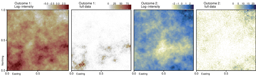
Figure 5: Log-intensity and corresponding synthetic count data at $14,400$ spatial locations for correlated spatial outcomes.

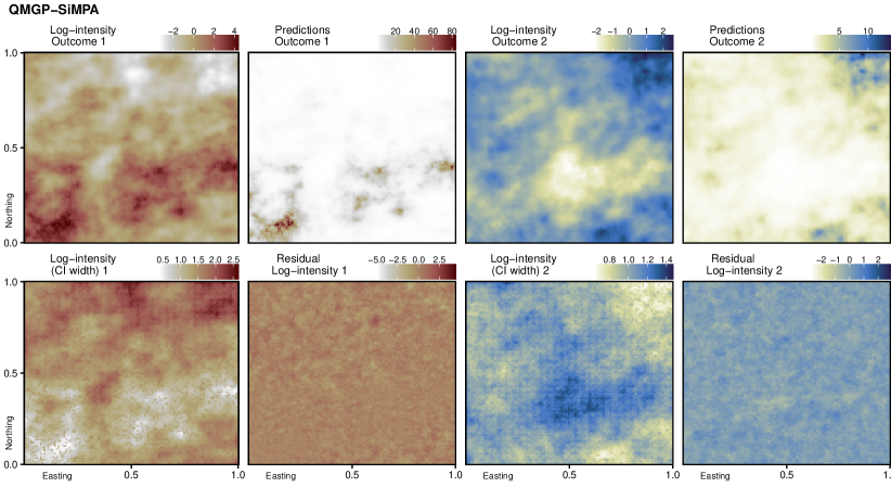
Figure 6: Output from fitting a coregionalized QMGP via SiMPA. Top row: recovered log-intensity and predictions for both outcomes. Bottom row: width of posterior credible intervals about log-intensity, and residual log-intensity.

We investigate the comparative performance of several coregionalized QMGP variants computed via MALA, SM-MALA, SiMPA and NUTS. We also consider latent multivariate Student-t processes (which we outline in the supplementary material, also see Chen et al., 2020; Shah et al., 2014) using an alternative cross-covariance specification based on Apanasovich and Genton, (2010)—in short “A&G10”—and previously used in Peruzzi et al., (2020), which we also implement in the meshed Gaussian case. We also compare with a data transformation method based on NNGPs: for each outcome, we use $y^{*}=log(1+y)$, then fit NNGP models of the response on each outcome independently. All MCMC-based models were fit on chains of length 30,000. Finally, we implement an MCMC-free stochastic partial differential equations method (SPDE; Lindgren et al., , 2011) fit via INLA. A summary of results from all implemented methods is available in Table 1, which reports root mean square prediction error (RMSPE) and mean absolute error in prediction (MAEP) when predicting the log-intensity $\eta_{j,\text{test}}$ and the outcomes $y_{j,\text{test}}$, $j=1,2$ on the test set of $5740$ locations, and the empirical coverage of 95% credible intervals (CI) about the log-intensity. Figure 7 expands on the analysis of empirical coverage of CIs by reporting the performance of all models at additional quantiles, relative to the oracle coverage (i.e. the empirical coverage of the model in which all unknowns are set to their true value). On the left subplots of Figure 7, a value near 1 implies that the empirical coverage of the $Q\%$ CI is close to the coverage of the true data generating model).

Langevin methods and NUTS for coregionalized QMGP outperformed other methods in all metrics for at least one outcome. However, NUTS had much slower compute times relative to simpler methods such as MALA and SiMPA, whereas SM-MALA exhibited slightly worse coverage. QMGPs based on LMCs outperformed those implemented with A&G10 cross-covariances, and a meshed Student-t process on a cubic DAG (QMTP) performed similarly to the analogous MGP using the same cross-covariance function. On the right of Figure 7, we report the rolling out-of-sample RMSPE in predicting $y_{j,\text{test}}$, $j=1,2$: QMGP-SiMPA predictions outperform SPDE-INLA starting from the 400th MCMC iteration—in other words, our proposed methodology led to good predictions for both outcomes in under 2.5 seconds in these contexts.

The comparison above is based on a single dataset; we replicate the same analysis on 750 smaller datasets. We target estimation of the latent correlation $\rho=\text{Corr}(w_{1}(\boldsymbol{\ell}),w_{2}(\boldsymbol{\ell}))$ in terms of absolute error and efficiency (ESS/s), along with the empirical coverage of 95% intervals about the log-intensity for both outcomes. Figure 8 summarizes our findings across the 750 datasets: Langevin methods, and in particular SiMPA, have low estimation error, high sampling efficiency, and excellent uncertainty quantification relative to all other tested methods. Additional details are available in the supplement.

Spatial proc.	SPDE		QMGP										QMTP		Univ. NNGP
Covariance	LMC										A&G10				Exponential
Compute	INLA		MALA		SM-MALA		SiMPA		NUTS						Resp/Transf
Outcome $\qquad j=$	1	2	1	2	1	2	1	2	1	2	1	2	1	2	1	2
$y_{j,\text{test}}(\boldsymbol{\ell})$ RMSPE	2.57	1.26	2.43	1.25	2.49	1.26	2.44	1.25	2.43	1.25	2.43	1.25	2.43	1.26	2.47	1.30
$y_{j,\text{test}}(\boldsymbol{\ell})$ MAEP	1.36	0.90	1.32	0.90	1.34	0.91	1.32	0.90	1.31	0.90	1.32	0.90	1.32	0.90	1.35	0.94
$\eta_{j,\text{test}}(\boldsymbol{\ell})$ RMSPE	0.42	0.22	0.41	0.23	0.46	0.27	0.41	0.23	0.41	0.23	0.41	0.23	0.42	0.23	1.19	0.85
$\eta_{j,\text{test}}(\boldsymbol{\ell})$ MAEP	0.33	0.18	0.32	0.18	0.36	0.21	0.32	0.18	0.32	0.18	0.33	0.18	0.33	0.18	0.92	0.68
$\eta_{j,\text{test}}(\boldsymbol{\ell})$ 95% Covg	0.79	0.85	0.94	0.97	0.94	0.98	0.94	0.97	0.94	0.97	0.87	0.93	0.81	0.91	0.61	0.77
Time (s)	217		149		223		166		530		280		550		207

Table 1: Summary of out-of-sample results for all implemented models. Bolded values correspond to best performance.

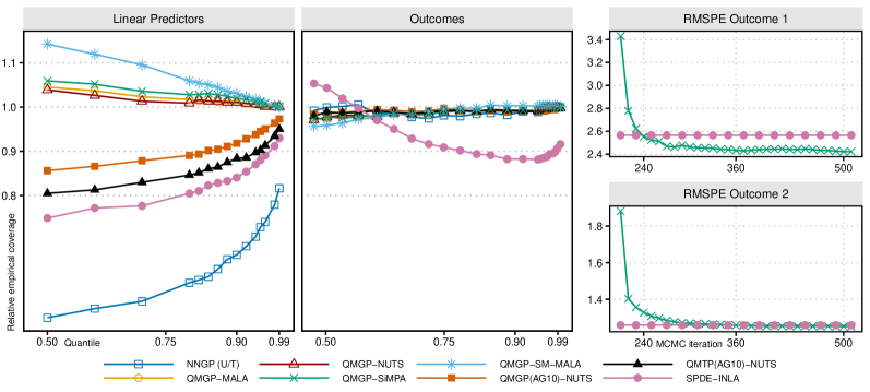
Figure 7: Left subplots: empirical coverage of uncertainty intervals at different quantiles, relative to the oracle model (values under 1 imply undercoverage of the interval). Right subplots: rolling RMSPE on both outcomes as a function of MCMC iteration–the RMSPE of the SPDE-INLA model is presented as a horizontal line.

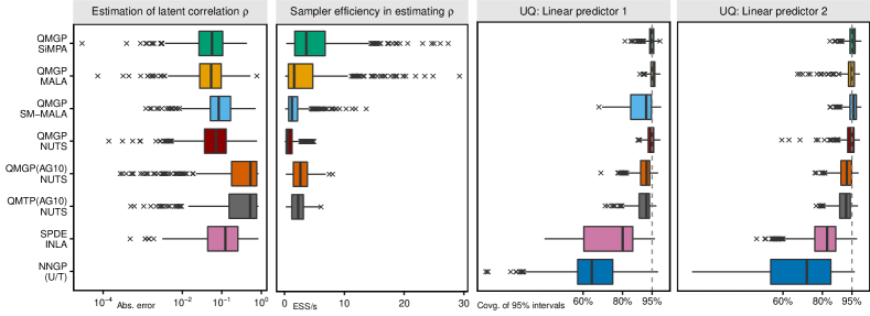
Figure 8: From the left: absolute error in estimation of $\rho$, efficiency in terms of ESS/s, and coverage of intervals about $\eta_{j,\text{test}}$, $j=1,2$, over 750 simulated datasets.

5.2 MODIS data: leaf area and snow cover

The dynamics of vegetation greenness are important drivers of ecosystem processes; in alpine regions, they are influenced by seasonal snow cover. Predictive models for vegetation greenup and senescence in these settings are crucial for understanding how local biological communities respond to global change (Walker et al., , 1993; Jönsson et al., , 2010; Wang et al., 2015a, ; Xie et al., , 2020). We consider remotely sensed leaf area and snow cover data from the MODerate resolution Imaging Spectroradiometer (MODIS) on the Terra satellite operated by NASA (v.6.1) at 122,500 total locations (a 350$\times$ 350 grid where each cell covers a 0.25km² area) over a region spanning northern Italy, Switzerland, and Austria, during the 8-day period starting on December 3rd, 2019 (Figure 1). Leaf area index (LAI; number of equivalent layers of leaves relative to a unit of ground area, available as level 4 product MOD15A2H) is our primary interest and is stored as a positive integer value but is missing or unavailable at 38.2% of all spatial locations due to cloud cover or poor measurement quality. Snow cover (SC; number of days within an 8-day period during which a location is covered by snow, obtained from level 3 product MOD10A2) is measured with error and missing at 7.3% of the domain locations.

We create a test set by introducing missingness in LAI at 10,000 spatial locations, of which 5030 are chosen uniformly at random across the whole domain and 4970 belong to a contiguous rectangular region as displayed on the bottom left subplot of Figure 9(a). We attempt to explain LAI based on SC by fitting (9) on the bivariate outcome $\boldsymbol{y}(\boldsymbol{\ell})=(y_{\text{SC}}(\boldsymbol{\ell}),y_{\text{LAI}}(\boldsymbol{\ell}))^{\top}$ where we assume a Binomial distribution with $8$ trials and logit link for SC, i.e. $E(y_{\text{SC}}(\boldsymbol{\ell})\mid\mu(\boldsymbol{\ell}))=8\mu(\boldsymbol{\ell})=8(1+\exp\{-\eta_{\text{SC}}(\boldsymbol{\ell})\})^{-1}$, and a Poisson or Negative Binomial distribution for LAI. In both cases, $E(y_{\text{LAI}}(\boldsymbol{\ell})\mid\eta_{\text{LAI}}(\boldsymbol{\ell}))=\mu_{\text{LAI}}(\boldsymbol{\ell})=\exp\{\eta_{\text{LAI}}(\boldsymbol{\ell})\}$; for the Poisson model, $Var(y_{\text{LAI}}(\boldsymbol{\ell})\mid\eta_{\text{LAI}}(\boldsymbol{\ell}))=\mu_{\text{LAI}}(\boldsymbol{\ell})$, whereas for the Negative Binomial model $Var(y_{\text{LAI}}(\boldsymbol{\ell})\mid\eta_{\text{LAI}}(\boldsymbol{\ell}))=\mu_{\text{LAI}}(\boldsymbol{\ell})+\tau\mu_{\text{LAI}}^{2}(\boldsymbol{\ell})$ where $\tau$ is an unknown scale parameter. We fit model (9) using latent coregionalized QMGPs with $k=2$ on a $50\times 50$ axis-parallel domain partition and run SiMPA for 30,000 iterations, of which 10,000 are discarded as burn-in and thinning the remaining ones with a 20:1 ratio, leading to a posterior sample of size 1,000. We compare our approaches in terms of prediction and uncertainty quantification about $y_{\text{LAI}}$ on the test set to a SPDE-INLA approach implemented on a $60\times 60$ mesh which led to similar compute times. As shown in Table 2, QMGP-SiMPA is competitive with or outperforms the SPDE-INLA method across all measured quantities. Figure 9(b) reports predictive maps of the tested models (prediction values are censored at 100 for visualization clarity), along with a visualization of 75% one-sided credible intervals which shows the SPDE-INLA method exhibiting undesirable spatial patterns, unlike QMGP-SiMPA.

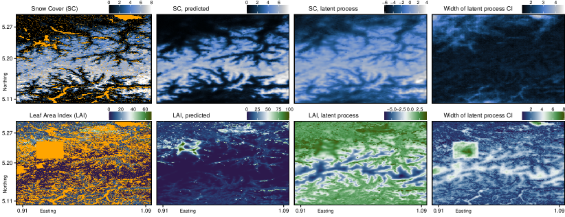
(a) From the left: in-sample data, predictions of outcomes and latent processes, uncertainty quantification from a QMGP-SiMPA model using a Poisson distribution for LAI.

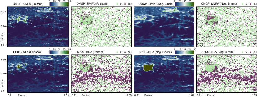
(b) Each raster image reports whole-domain predictions of all tested models, whereas each dark dot in the point clouds represents a domain location at which the 75% one-sided credible interval does not include the observed data point.

Figure 9: Performance of QMGP-SiMPA and SPDE-INLA in the MODIS data application.

Method	$F_{\text{LAI}}$	RMSPE	MedAE	CRPS		$CI_{75}$	$CI_{95}$	$CI_{99}$	Time
				(mean)	(median)				(minutes)
QMGP-SiMPA	Poisson	17.398	1.399	3.859	1.205	0.882	0.978	0.990	22.2
	Neg. Binom.	12.279	2.235	4.482	2.312	0.812	0.980	0.995	27.9
SPDE-INLA	Poisson	27.839	2.154	4.695	1.214	0.835	0.938	0.961	25.8
	Neg. Binom.	27019.470	2.444	54.986	1.720	0.875	0.975	0.987	86.5

Table 2: Root mean square error (RMSPE), median absolute error (MedAE), continuous ranked probability score (CRPS), and empirical coverage of one-sided intervals ($CI_{q}$), over the out-of-sample test set of 6,998 locations.

6 Application: spatial community ecology

Ecologists seek to jointly model the spatial occurrence of multiple species, while inferring the impact of phylogeny and environmental covariates. In order to realistically model such a scenario, we consider cases in which a relatively large number of georeferenced outcomes is observed, with the goal of predicting their realization at unobserved locations and estimating their latent correlation structure after accounting for spatial and/or temporal variability. Presence/absence information for different species is encoded as a multivariate binary outcome. Throughout this section, our model for multivariate outcomes lets $F_{j}(y_{j}(\boldsymbol{\ell});\eta_{j}(\boldsymbol{\ell}))=Bern(\mu_{j}(\boldsymbol{\ell}))$ where $\mu_{j}(\boldsymbol{\ell})=(1+\exp\{-\eta_{j}(\boldsymbol{\ell})\})^{-1}$ and $v_{h}(\cdot)\sim QMGP(\mathbf{0},\boldsymbol{\rho}_{h}(\cdot,\cdot)),h=1,\dots,k$ in model (9), leading to coregionalized $k$-factor QMGPs which we fit via several Langevin methods, all of which use domain partitioning with blocks of size $\approx 36$ and independent standard Gaussian priors on the lower-triangular elements of the factor loadings $\boldsymbol{\Lambda}$, unless otherwise noted.

We compare QMGP methods fit via our proposed Langevin algorithms to joint species distribution models (JSDM) implemented in R package Hmsc (Tikhonov et al., , 2020), a popular software package for community ecology. Hmsc uses a probit link for binary outcomes, i.e. $\mu_{j}(\boldsymbol{\ell})=\Phi(\eta_{j}(\boldsymbol{\ell}))$ where $\Phi(\cdot)$ is the Gaussian distribution function; then, non-spatial JSDMs are implemented by letting $v_{h}(\boldsymbol{\ell})\sim N(0,1)$ independently for all $\boldsymbol{\ell}$ and $h=1,\dots,K$, whereas NNGP-based JSDMs assume $v_{h}(\cdot)\sim NNGP(\mathbf{0},\boldsymbol{\rho}_{h}(\cdot,\cdot)),h=1,\dots,k$. We set the number of neighbors as $m=20$ in the NNGP specification. Hmsc assumes a cumulative shrinkage prior on the factor loadings (Bhattacharya and Dunson, , 2011), which we set up with minimal shrinking ($a_{1}=2,a_{2}=2$) unless otherwise noted.

6.1 Synthetic data

We generate 30 datasets by sampling $q=10$ binary outcomes at $n=900$ locations scattered uniformly in the domain $[0,1]^{2}$: after sampling $k=3$ independent univariate GPs $v_{j}(\cdot)\sim GP(\mathbf{0},C_{\varphi_{j}})$ where $C_{\varphi_{j}}(\boldsymbol{\ell},\boldsymbol{\ell}^{\prime})=\exp\{-\varphi_{j}\|\boldsymbol{\ell}-\boldsymbol{\ell}^{\prime}\|\}$ is the exponential covariance function with decay parameter $\varphi_{j}$, we construct a $q$-variate GP via coregionalization by letting $\boldsymbol{w}(\boldsymbol{\ell})=\boldsymbol{\Lambda}\boldsymbol{v}(\boldsymbol{\ell})$ where $\boldsymbol{\Lambda}$ is a $q\times k$ lower-triangular matrix. We then sample the binary outcomes using a probit link, i.e. $y_{j}(\boldsymbol{\ell})\sim Bern(\mu_{j}(\boldsymbol{\ell}))$ where $\mu_{j}(\boldsymbol{\ell})=\Phi(\boldsymbol{x}(\boldsymbol{\ell})^{\top}\bbeta_{j}+w_{j}(\boldsymbol{\ell}))$ for each $j=1,\dots,q$ and where $\boldsymbol{x}(\boldsymbol{\ell})$ is a column vector of $p=2$ covariates. For each of the 30 datasets, we randomly set $\varphi_{j}\sim U(1/2,10),j=1,\dots,k$, $\boldsymbol{\Lambda}_{jj}\sim U(3/2,2)$ for $j=1,\dots,k$, $\boldsymbol{\Lambda}_{ij}\sim U(-2,2)$ for $i<j$, and $\bbeta_{j}\sim N(\mathbf{0},I_{2}/5)$. These choices lead to a wide range of latent pairwise correlations induced on the outcomes via $\boldsymbol{w}(\cdot)$: letting $\boldsymbol{\Omega}=(\omega_{ij})_{i,j=1,\dots,q}=\boldsymbol{\Lambda}\boldsymbol{\Lambda}^{\top}$ represent the cross-covariance at zero spatial distance, we find the cross-correlations as $\boldsymbol{\Omega}_{\text{corr}}=\text{diag}(\omega_{jj}^{-1/2})\boldsymbol{\Omega}\text{diag}(\omega_{jj}^{-1/2})$. We realistically model long-range spatial dependence by choosing small values for $\varphi_{j}$, $j=1,\dots,k$. Lastly, we create a test set using 20% of the locations for each outcome (missing data locations differ for each outcome).

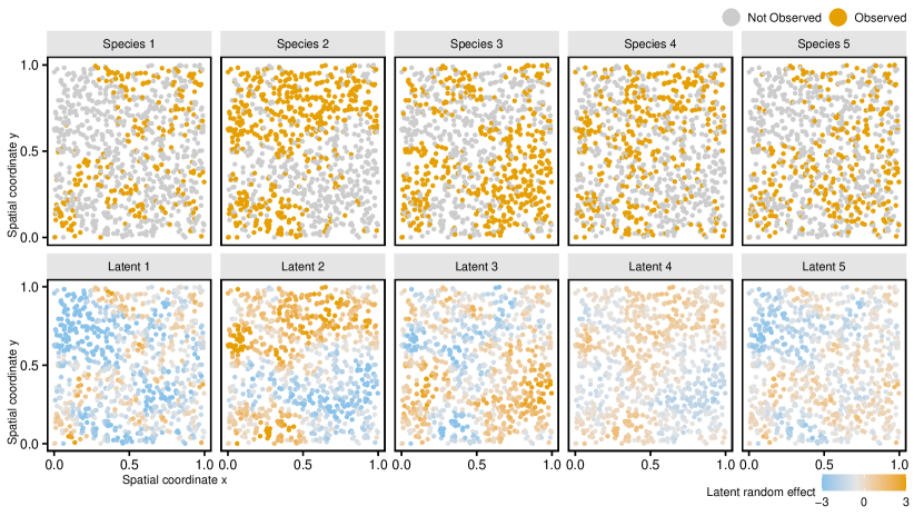
Figure 10: Synthetic dichotomous occurrence data (top row), and the spatial latent effects used to generate them (bottom row). Here, we show 5 (of 10) outcomes in 1 (of 30) simulated datasets.

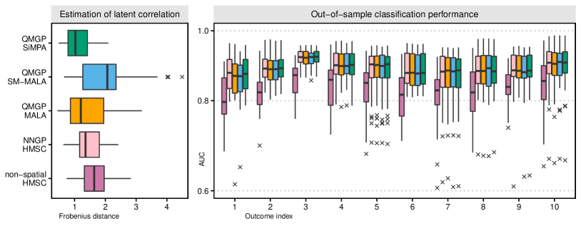
Figure 11: Box-plot summaries of estimation and classification performance over 30 datasets. Left: $\|\hat{\Omega}_{\text{corr}}-\Omega_{\text{corr}}\|_{F}$ for the competing methods. Right: AUC for each outcome.

We use the setup of QMGPs and Hmsc outlined above, noting that the link function used to generate the data is correctly specified for Hmsc but not for our models based on QMGP due to our current software implementation in R package meshed. MCMC for all methods was run for 10,000 iterations, of which the first 5,000 is discarded as burn-in. We compare all models based on the out-of-sample classification performance on each of the 10 outcomes as measured via the area under the receiver operating characteristic curve (AUC). Since a primary interest in these settings is to estimate latent correlations across outcomes, we compare models based on $\|\hat{\Omega}_{\text{corr}}-\Omega_{\text{corr}}\|_{F}$, i.e. the Frobenius distance between the Monte Carlo estimate of cross-correlation and its true value. Therefore, smaller values of $\|\hat{\Omega}_{\text{corr}}-\Omega_{\text{corr}}\|_{F}$ are desirable. Figure 11 shows box-plots summarising the results, whereas Table 3 reports averages along with compute times. In these settings, the non-spatial model unsurprisingly performed worst. Langevin methods for the spatial models proposed in this article – and in particular SiMPA – lead to improved classification performance, smaller errors in estimating latent correlations, and a 27-fold reduction in compute time, relative to the coregionalized NNGP method implemented via MCMC in Hmsc.

Method	Hmsc		MALA	SM-MALA	SiMPA
Prior on rand. eff.	non-spatial	NNGP	QMGP
Avg. AUC	0.827	0.885	0.882	0.881	0.885
Min. AUC	0.573	0.608	0.600	0.607	0.609
Max. AUC	0.969	0.983	0.985	0.985	0.985
$\|\hat{\Omega}_{\text{corr}}-\Omega_{\text{corr}}\|_{F}$	1.66	1.43	1.47	2.04	1.12
Avg. time (minutes)	5.22	16.3	0.47	0.76	0.59

Table 3: Performance in classification, estimation, and compute time, over 30 synthetic datasets.

6.2 North American breeding bird survey data

The North American Breeding Bird Survey dataset contains avian point count data for more than 700 North American bird taxa (species, races, and unidentified species groupings). These data are collected annually during the breeding season, primarily June, along thousands of randomly established roadside survey routes in the United States and Canada.

We consider a dataset of $n=4118$ locations spanning the continental U.S., and $q=27$ bird species. The specific species we consider belong to the passeriforme order and are observed at a number of locations which is between 40% and 60% of the total number of available locations – Figure 2 shows a subset of the data. We dichotomize the observed counts to obtain presence/absence data. The effective data size is $nq=$ 111,186. We implement Langevin methods using coregionalized QMGPs with $k=2,4,6,8,10$ spatial factors using exponential correlations with decay $\phi\sim U[0.1,10]$ a priori. We also test the sensitivity to the domain partitioning scheme by testing $8\times 4$ (coarse), $16\times 8$ (medium), and $32\times 16$ (fine) axis-parallel domain partitioning schemes. Finer partitioning implies more restrictive spatial conditional independence assumptions. In implementing the shrinkage prior of Bhattacharya and Dunson, (2011), Hmsc dynamically chooses the number of factors up to a maximum $k_{\text{max}}$: in the non-spatial Hmsc model, letting $k_{\text{max}}=10$ ultimately leads to 6 or fewer factors being used during MCMC. In the spatial Hmsc models using NNGPs, we set $k_{\text{max}}=2$ or $k_{\text{max}}=5$ to restrict run times. Figure 12 reports average classification performance and run times. QMGP-MALA scales only linearly with the number of factors, but its performance is strongly negatively impacted by partition size. QMGP-SM-MALA exhibits large improvements in classification performance, however these improvements come at a large run time cost. Performance of SM-MALA also slightly worsens with a coarser partition due to the increased dimension of the sampled targets. On the contrary, QMGP-SiMPA outperforms all other models while providing large time savings relative to SM-MALA and being less sensitive to the choice of partition. A QMGP-SiMPA model on the $32\times 16$ partition with $k=4$ outperforms a spatial NNGP-Hmsc model in classifying the 27 bird species with a reduction in run time of over three orders of magnitude (respectively 4.1 minutes and 70.7 hours). We provide a summary of the efficiency in sampling the elements of $\boldsymbol{\Omega}_{\text{corr}}$ in Table 4, where we make comparisons of ESS/s relative to the non-spatial Hmsc model. While efficient estimation of $\boldsymbol{\Omega}_{\text{corr}}$ remains challenging, QMGP-SiMPA models show marked improvements relative to a state-of-the-art alternative.

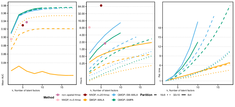
Figure 12: Left: mean AUC across the 27 bird species for different choices of $k$. Center: run times in hours. Right: run time of QMGP models as a proportion to the run time choosing $k=2$.

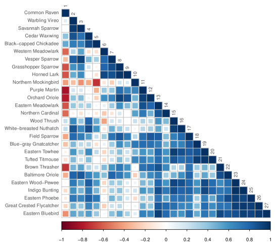
Figure 13: Lower triangular portion of $\boldsymbol{\Omega}_{\text{corr}}$, the estimated correlation among the 27 bird species.

Method	Hmsc		SiMPA
Prior	non-spatial	NNGP	QMGP
$k$	$\leq 10$	5	4	4	10	10
Setting		$m=20$	$32\times 16$	$8\times 4$	$32\times 16$	$8\times 4$
Avg. AUC	0.9349	0.9293	0.9544	0.9562	0.9729	0.9741
Time (minutes)	87.45	4245.02	4.17	56.77	10.95	295.23
ESS/s for elements of $\boldsymbol{\Omega}_{\text{corr}}$ (relative to Hmsc non-spatial)
min	1	$10^{-4}$	0.54	0.02	0.06	0.002
median	1	0.012	2.98	0.19	0.96	0.020
mean	1	0.015	4.26	0.33	1.28	0.032
max	1	0.102	29.61	4.08	8.84	0.406

Table 4: Out-of-sample performance in classification of the 27 bird species, compute time, and efficiency in estimation of $\boldsymbol{\Omega}_{\text{corr}}$, relative to a non-spatial JDSM model.

7 Discussion

We have introduced Bayesian hierarchical models based on DAG constructions of latent spatial processes for large scale non-Gaussian multivariate multi-type data which may be misaligned, along with computational tools for adaptive posterior sampling.

We have applied our methodologies using practical cross-covariance choices such as models of coregionalization built on independent stationary covariances. However, nonstationary models are desirable in many applied settings. Recent work (Jin et al., , 2021) highlights that DAG choice must be made carefully when considering explicit models of nonstationary, as spatial process models based on sparse DAGs induce nonstationarities even when using stationary covariances. Our work in this article will enable new research into nonstationary models of large scale non-Gaussian data. Furthermore, our methods can be applied for posterior sampling of Bayesian hierarchies based on more complex conditional independence models of multivariate dependence (Dey et al., , 2021).

Our methodologies rely on the ability to embed the assumed spatial DAG within the larger Bayesian hierarchy and lead to drastic reductions in wall clock time compared to models based on unrestricted GPs. Nevertheless, high posterior correlations of high dimensional model parameters may still negatively impact overall sampling efficiency in certain cases. Motivated by recent progress in improving sampling efficiency of multivariate Gaussian models (Peruzzi et al., , 2021), future research will consider generalized strategies for improving MCMC performance in spatial factor models of highly multivariate non-Gaussian data. Finally, optimizing DAG choice for MCMC performance is another interesting path, and recent work on the theory of Bayesian computation for hierarchical models (Zanella and Roberts, , 2021) might motivate further development for spatial process models based on DAGs.

Acknowledgements

The authors have received funding from the European Research Council (ERC) under the European Union’s Horizon 2020 research and innovation programme (grant agreement No 856506), and grant R01ES028804 of the United States National Institutes of Health (NIH)

Supplementary Material

Appendix A Spatial meshing with projections

The customary setup of a DAG-based model based on spatial meshing is to let ${\cal S}\cap{\cal T}\approx{\cal T}$ as the resulting large overlap between knots and observed locations avoids sampling at non-reference locations. However, it is often desirable to allow flexible choices of ${\cal S}$; for example, there are some computational advantages when ${\cal S}$ is a grid and ${\cal T}$ are irregularly spaced, or when the data are observed with particular patterns (Peruzzi et al., , 2021). In order to let ${\cal S}$ be more flexibly determined while also avoiding sampling $\boldsymbol{w}(\boldsymbol{\ell})$ at non-reference locations, we introduce a linear projection operator $\boldsymbol{H}(\boldsymbol{\ell})$ of dimension $q\times qn_{[\boldsymbol{\ell}]}$ and where $n_{[\boldsymbol{\ell}]}$ is the number of locations in $[\boldsymbol{\ell}]\subset{\cal S}$; after denoting $\widetilde{\boldsymbol{w}}(\boldsymbol{\ell})=\boldsymbol{H}(\boldsymbol{\ell})\boldsymbol{w}_{[\boldsymbol{\ell}]}$, we assume that if $\boldsymbol{\ell}\in{\cal S}$ then $\boldsymbol{H}(\boldsymbol{\ell})$ is such that $\widetilde{\boldsymbol{w}}(\boldsymbol{\ell})=\boldsymbol{w}(\boldsymbol{\ell})$. Then, we build the outcome model as

$$y_{j}(\boldsymbol{\ell})\,|\,\eta_{j}(\boldsymbol{\ell}),\gamma_{j} \sim F_{j}(\eta_{j}(\boldsymbol{\ell}),\gamma_{j}),\qquad\eta_{j}(\boldsymbol{\ell})=\boldsymbol{x}_{j}(\boldsymbol{\ell})^{\top}\bbeta_{j}+\widetilde{w}_{j}(\boldsymbol{\ell}),$$ (12)

$$\boldsymbol{w}(\cdot) \sim\Pi_{{\cal G}}$$

where we have replaced $\boldsymbol{w}(\boldsymbol{\ell})$ with $\widetilde{\boldsymbol{w}}(\boldsymbol{\ell})$. Setting $\boldsymbol{H}(\boldsymbol{\ell})$ such that $\widetilde{\boldsymbol{w}}(\boldsymbol{\ell})=E[\boldsymbol{w}(\boldsymbol{\ell})\,|\,\boldsymbol{w}_{[\boldsymbol{\ell}]}]$ leads to an interpretation of (12) as a “local” predictive process (Banerjee et al., , 2008). The posterior distribution for this model is:

$$\pi(\{\bbeta_{j},\gamma_{j}\}_{j=1}^{q},\boldsymbol{w}_{{\cal S}},\boldsymbol{\theta}\,|\,\boldsymbol{y}_{{\cal T}}) \propto\pi(\boldsymbol{\theta})\pi_{{\cal G}}(\boldsymbol{w}_{\cal S}\,|\,\boldsymbol{\theta})\prod_{j=1}^{q}\pi(\bbeta_{j},\gamma_{j})\prod_{\boldsymbol{\ell}\in{\cal T}_{j}}dF_{j}(y_{j}(\boldsymbol{\ell})\,|\,\widetilde{w}_{j}(\boldsymbol{\ell}),\bbeta_{j}(\boldsymbol{\ell}),\gamma_{j}).$$ (13)

In this scenario, omitting the residual term $\boldsymbol{e}(\boldsymbol{\ell})=\boldsymbol{w}(\boldsymbol{\ell})-\widetilde{\boldsymbol{w}}(\boldsymbol{\ell})$ from (12) leads to advantages in sampling, but possible oversmoothing of the latent spatial surface due to the fact that $\text{var}[\widetilde{\boldsymbol{w}}(\boldsymbol{\ell})]<\text{var}[\boldsymbol{w}(\boldsymbol{\ell})]$. In the conditionally conjugate Gaussian setting, such biases can be partly corrected (Banerjee et al., , 2010; Peruzzi et al., , 2021). Certain ad-hoc solutions may be available by allowing spatial variation of $\gamma_{j}$, i.e. replacing it with $\gamma_{j}(\boldsymbol{\ell})$. However, we may choose to ignore the residual term because (1) it is common to assume smoother surfaces with non-Gaussian data, (2) we can choose ${\cal S}$ to be very large, reducing possible biases, (3) we can revert to model (1) by setting ${\cal S}={\cal T}$. Posterior sampling for (12) proceeds via Algorithm 4.

Algorithm 4 Posterior sampling of model (12).

1:Initialize $\bbeta_{j}^{(0)}$ and $\gamma_{j}^{(0)}$ for $j=1,\dots,q$, $\boldsymbol{w}_{{\cal S}}^{(0)}$, and $\boldsymbol{\theta}^{(0)}$

2:for $t\in\{1,\dots,T^{*},T^{*}+1,\dots,T^{*}+T\}$ do $\triangleright$ MCMC loop

3:     for $j=1,\dots,q$, sample $\bbeta_{j}^{(t)}\,|\,\boldsymbol{y}_{\cal T},\widetilde{\boldsymbol{w}}_{{\cal T}}^{(t-1)},\gamma_{j}^{(t-1)}$

4:     for $j=1,\dots,q$, sample $\gamma_{j}^{(t)}\,|\,\boldsymbol{y}_{\cal T},\widetilde{\boldsymbol{w}}_{{\cal T}}^{(t-1)},\bbeta_{j}^{(t)}$

5:     sample $\boldsymbol{\theta}^{(t)}\,|\,\boldsymbol{y}_{{\cal T}},\boldsymbol{w}^{(t-1)}_{{\cal S}},\{\bbeta_{j}^{(t)},\gamma_{j}^{(t)}\}_{j=1}^{q}$

6:     for $i=1,\dots,M$, sample $\boldsymbol{w}_{i}^{(t)}\,|\,\boldsymbol{w}_{\texttt{mb}(i)}^{(t)},\boldsymbol{y}_{i},\boldsymbol{\theta}^{(t)},\{\bbeta_{j}^{(t)},\gamma_{j}^{(t)}\}_{j=1}^{q}$ $\triangleright$ reference sampling

7:end for

8:Assuming convergence has been attained after $T^{*}$ iterations:

9:discard $\{\bbeta_{j}^{(t)},\gamma_{j}^{(t)}\}_{j=1}^{q},\boldsymbol{w}_{{\cal S}}^{(t)},\boldsymbol{\theta}^{(t)}$ for $t=1,\dots,T^{*}$

10:Output: Correlated sample of size $T$ with density

$$\{\bbeta_{j}^{(t)},\gamma_{j}^{(t)}\}_{j=1}^{q},\boldsymbol{w}_{{\cal S}}^{(t)},\boldsymbol{\theta}^{(t)}\sim\pi(\{\bbeta_{j},\gamma_{j}\}_{j=1}^{q},\boldsymbol{w}_{{\cal S}}^{(t)},\boldsymbol{\theta}\mid\boldsymbol{y}_{{\cal T}}).$$

Figure 14: Directed acyclic graph representing a special case of model (12), for locations at which at least one outcome is observed. For simplicity, we consider ${\cal S}\cap{\cal T}=\emptyset$ and omit the directed edges from $(\bbeta_{j},\gamma_{j})$ to each $y_{j}(\boldsymbol{\ell})$. If $y_{j}(\boldsymbol{\ell})$ is unobserved and therefore $\boldsymbol{\ell}\notin{\cal T}_{j}$, the corresponding node is missing.

Appendix B Choice of DAG and partition

Figure 15: Illustration of the two partitioning schemes. On the right, we juxtapose the second partitioning scheme to clarify the changes relative to the scenario on the left.

Spatially meshed models on the same partition of ${\cal S}$ can be compared in terms of the sparsity of ${\cal G}$. If edges are added to a sparse DAG ${\cal G}_{1}$ to obtain ${\cal G}_{2}$, the child process $\Pi_{{\cal G}_{2}}$ is closer to the parent process $\Pi_{\boldsymbol{\theta}}$ (in a Kullback-Leibler (KL) sense) relative to $\Pi_{{\cal G}_{1}}$ (Peruzzi et al., , 2020). For treed DAGs and recursive domain partitioning, the KL divergence of $\Pi_{{\cal G}}$ from $\Pi$ can be reduced by increasing the block size at the root nodes (Peruzzi and Dunson, , 2021). Here, we analyse the modeling implications different non-nested domain partitions have, while using the same DAG structure to govern dependence between partition regions. This scenario occurs e.g. when constructing a cubic MGP model (QMGP).

We consider two partitions of the x-coordinate axis within a $2\times 2$ axis-parallel partitioning scheme (Figure 15) and construct $\Pi_{{\cal G}}^{(i)}$, $i=1,2$ based on each partitioning scheme. According to the first partitioning scheme, $\boldsymbol{w}_{{\cal S}}$ (in short, $\boldsymbol{w}$) is partitioned as $\boldsymbol{w}=\{\boldsymbol{w}_{1},\boldsymbol{w}_{2},\boldsymbol{w}_{3},\boldsymbol{w}_{4}\}$ whereas with the alternative we have $\boldsymbol{w}=\{\boldsymbol{w}_{1}^{*},\boldsymbol{w}_{2,2},\boldsymbol{w}_{3}^{*},\boldsymbol{w}_{4,2}\}$ where $\boldsymbol{w}_{1}^{*}=\{\boldsymbol{w}_{1},\boldsymbol{w}_{2,1}\}$ and $\boldsymbol{w}_{3}^{*}=\{\boldsymbol{w}_{3},\boldsymbol{w}_{4,1}\}$. When analysing the relative KL divergence of these two models from $\Pi$, we see

$$KL(\pi\|\pi_{{\cal G}}^{(2)})-KL(\pi\|\pi_{{\cal G}}^{(1)}) =\int\log\frac{\pi(\boldsymbol{w})}{\pi_{{\cal G}}^{(2)}(\boldsymbol{w})}\pi(\boldsymbol{w})d\boldsymbol{w}-\int\log\frac{\pi(\boldsymbol{w})}{\pi_{{\cal G}}^{(1)}(\boldsymbol{w})}\pi(\boldsymbol{w})d\boldsymbol{w}$$

$$=\int\log\pi_{{\cal G}}^{(1)}(\boldsymbol{w})\pi(\boldsymbol{w})d\boldsymbol{w}-\int\log\pi_{{\cal G}}^{(2)}(\boldsymbol{w})\pi(\boldsymbol{w})d\boldsymbol{w}$$

$$=\int\left(\log\pi_{{\cal G}}^{(1)}(\boldsymbol{w})-\log\pi_{{\cal G}}^{(2)}(\boldsymbol{w})\right)\pi(\boldsymbol{w})d\boldsymbol{w}$$

Since we fix the same ${\cal G}$ across partitions, we have

$$\pi_{{\cal G}}^{(1)}(\boldsymbol{w}_{\cal S}) =\pi(\boldsymbol{w}_{1})\pi(\boldsymbol{w}_{2}\,|\,\boldsymbol{w}_{1})\pi(\boldsymbol{w}_{3}\,|\,\boldsymbol{w}_{1})\pi(\boldsymbol{w}_{4}\,|\,\boldsymbol{w}_{2},\boldsymbol{w}_{3})$$

$$=\pi(\boldsymbol{w}_{1})\pi(\boldsymbol{w}_{2,1}\,|\,\boldsymbol{w}_{1})p(\boldsymbol{w}_{2,2}\,|\,\boldsymbol{w}_{1},\boldsymbol{w}_{2,1})\pi(\boldsymbol{w}_{3}\,|\,\boldsymbol{w}_{1})\pi(\boldsymbol{w}_{4,1}\,|\,\boldsymbol{w}_{2,1},\boldsymbol{w}_{2,2},\boldsymbol{w}_{3})\ \cdot$$

$$\qquad\cdot\ \pi(\boldsymbol{w}_{4,2}\,|\,\boldsymbol{w}_{2,1},\boldsymbol{w}_{2,2},\boldsymbol{w}_{3},\boldsymbol{w}_{4,1})$$

$$\pi_{{\cal G}}^{(2)}(\boldsymbol{w}_{\cal S}) =\pi(\boldsymbol{w}_{1}^{*})\pi(\boldsymbol{w}_{2,2}\,|\,\boldsymbol{w}_{1}^{*})\pi(\boldsymbol{w}_{3}^{*}\,|\,\boldsymbol{w}_{1}^{*})\pi(\boldsymbol{w}_{4,2}\,|\,\boldsymbol{w}_{2,2},\boldsymbol{w}_{3}^{*})$$

$$=\pi(\boldsymbol{w}_{1})\pi(\boldsymbol{w}_{2,1}\,|\,\boldsymbol{w}_{1})p(\boldsymbol{w}_{2,2}\,|\,\boldsymbol{w}_{1},\boldsymbol{w}_{2,1})\pi(\boldsymbol{w}_{3}\,|\,\boldsymbol{w}_{1},\boldsymbol{w}_{2,1})\pi(\boldsymbol{w}_{4,1}\,|\,\boldsymbol{w}_{1},\boldsymbol{w}_{2,1},\boldsymbol{w}_{3})\ \cdot$$

$$\qquad\cdot\ \pi(\boldsymbol{w}_{4,2}\,|\,\boldsymbol{w}_{2,2},\boldsymbol{w}_{3},\boldsymbol{w}_{4,1}),$$

and therefore the sign of $KL(\pi\|\pi_{{\cal G}}^{(2)})-KL(\pi\|\pi_{{\cal G}}^{(1)})$ depends on

$$\log\frac{\pi_{{\cal G}}^{(1)}(\boldsymbol{w})}{\pi_{{\cal G}}^{(2)}(\boldsymbol{w})} =\log\left(\frac{\pi(\boldsymbol{w}_{3}\,|\,\boldsymbol{w}_{1})}{\pi(\boldsymbol{w}_{3}\,|\,{\color[rgb]{0,.5,.5}\boldsymbol{w}_{2,1}},\boldsymbol{w}_{1})}\frac{\pi(\boldsymbol{w}_{4,1}\,|\,{\color[rgb]{0,.5,.5}\boldsymbol{w}_{2,2}},\boldsymbol{w}_{2,1},\boldsymbol{w}_{3})}{\pi(\boldsymbol{w}_{4,1}\,|\,{\color[rgb]{0,.5,.5}\boldsymbol{w}_{1}},\boldsymbol{w}_{2,1},\boldsymbol{w}_{3})}\frac{\pi(\boldsymbol{w}_{4,2}\,|\,{\color[rgb]{0,.5,.5}\boldsymbol{w}_{2,1}},\boldsymbol{w}_{2,2},\boldsymbol{w}_{3},\boldsymbol{w}_{4,1})}{\pi(\boldsymbol{w}_{4,2}\,|\,\boldsymbol{w}_{2,2},\boldsymbol{w}_{3},\boldsymbol{w}_{4,1})}\right),$$

where we see that the performance of $\Pi_{{\cal G}}^{(1)}$ relative to $\Pi_{{\cal G}}^{(2)}$ in approximating $\Pi$ is undetermined because there is no ordering between the number of edges in $\Pi_{{\cal G}}^{(1)}$ and $\Pi_{{\cal G}}^{(2)}$. Nevertheless, the above discussion remains useful in practice when the reference set ${\cal S}$ is chosen at observed locations. For example, if data are unavailable at $(2,1)$, then $\boldsymbol{w}_{2,1}$ has length zero, and one would then choose $\Pi_{{\cal G}}^{(1)}$ over $\Pi_{{\cal G}}^{(2)}$ if uncertainty about $\boldsymbol{w}_{4,1}$ is reduced by knowledge of $\boldsymbol{w}_{2,2}$ more than it is reduced by knowledge of $\boldsymbol{w}_{1}$.

Appendix C Alternative latent processes and sampling methods

We have concentrated our focus in the main article on latent GPs and Langevin sampling methods, but the methods we propose are more general and we provide further examples here.

C.1 Spatial meshing of Student-t processes

GPs are desirable thanks to their convenient properties; however, a similar construction based on cross-covariances can be used to model $\boldsymbol{w}(\cdot)$ as a $q$-variate Student-t process (TP), in which case we write $\boldsymbol{w}(\boldsymbol{\ell})\sim TP_{\nu_{0}}(\mathbf{0},\boldsymbol{C}(\cdot,\cdot))$ where $\nu_{0}>2\in\Re$ is a degrees of freedom parameter which controls tail heaviness; similarities with GPs include closedness under marginalization and analytic forms of conditional densities. Then, for any ${\cal L}$, the random effects have a multivariate Student-t distribution, i.e. $\boldsymbol{w}_{{\cal L}}\sim MVT_{\nu_{0}}(0,\boldsymbol{C}_{{\cal L}})$. In the limiting case $\nu_{0}\to\infty$ one obtains a GP with cross-covariance $\boldsymbol{C}(\cdot,\cdot)$. Shah et al., (2014) and Chen et al., (2020) introduce and consider TPs as alternatives to GPs in regression, citing improved flexibility owing to the ability of a TP to capture more extreme behavior. There are difficulties associated to using TPs in regression, notably the lack of closedness under linear combinations. This implies that spatial meshing of multivariate TPs built upon a LMC does not equate the LMC of spatially meshed univariate TPs.

The TP is closed under marginalization and conditioning, which implies that it is relatively easy to build a spatially meshed TP. Letting $\boldsymbol{w}_{\cal L}=\boldsymbol{w}$ and $\boldsymbol{C}_{\cal L}=\boldsymbol{C}$ for simplicity, the density of a zero-mean TP evaluated at $\boldsymbol{w}$, denoted as $MVT(\nu,\mathbf{0},\boldsymbol{C})$ is defined as (Shah et al., , 2014)

$$p(\boldsymbol{w}\,|\,\nu_{0}) =\frac{\Gamma(\frac{\nu+n}{2})}{((\nu-2)\pi)^{n/2}}|\boldsymbol{C}|^{-\frac{1}{2}}\left(1+\frac{1}{\nu-2}\boldsymbol{w}^{\top}\boldsymbol{C}^{-1}\boldsymbol{w}\right)^{-\frac{\nu+n}{2}}.$$

The above density formulation leads to $\text{cov}(\boldsymbol{w})=\boldsymbol{C}$. Closedness of the TP under marginalization and conditioning leads to the TP conditional densities also being multivariate t’s; we find

$$\pi(\boldsymbol{w}_{i}\,|\,\boldsymbol{w}_{[i]}) \sim MVT\left(\nu+n_{[i]},\boldsymbol{H}_{i}\boldsymbol{w}_{[i]},\frac{\boldsymbol{b}+\nu-2}{n_{[i]}+\nu-2}\boldsymbol{R}_{i}\right),$$

where $\boldsymbol{H}_{i}$ and $\boldsymbol{R}_{i}$ are defined like in the GP, and the new term $\boldsymbol{b}=\boldsymbol{w}_{[i]}^{\top}\boldsymbol{C}^{-1}_{[i]}\boldsymbol{w}_{[i]}$ determines how the conditional variance of $\boldsymbol{w}_{i}\,|\,\boldsymbol{w}_{[i]}$ also depends on the values of $\boldsymbol{w}_{[i]}$. In fact, $\text{cov}(\boldsymbol{w}_{i}\,|\,\boldsymbol{w}_{[i]})=\frac{\boldsymbol{b}+\nu-2}{n_{[i]}+\nu-2}\boldsymbol{R}_{i}$, where the (covariance-weighted) sum of squares $\boldsymbol{b}$ is used to inform the conditional density about the observed variance in the conditioning set. In fact, $\boldsymbol{b}/n_{[i]}$ is large (i.e., the conditioning set has larger spread), then the conditional variance is also larger. This intuitive behavior is missing from a GP, which we obtain in this context by letting $\nu\to\infty$ (or $n_{[i]}\to\infty$, which is uninteresting when doing spatial meshing).

C.1.1 Gradient based sampling for MTPs

When building gradient-based MCMC methods for posterior sampling MTPs, we require $\nabla_{\boldsymbol{w}_{i}}\log p(\boldsymbol{w}_{i}\,|\,\textrm{---})=\boldsymbol{f}_{i}+\frac{\delta}{\delta\boldsymbol{w}_{i}}\log p(\boldsymbol{w}_{i}\,|\,\boldsymbol{w}_{[i]},\boldsymbol{\theta})+\sum_{j\to\{i\to j\}}\frac{\delta}{\delta\boldsymbol{w}_{i}}\log p(\boldsymbol{w}_{j}\,|\,\boldsymbol{w}_{i},\boldsymbol{w}_{[j]\setminus\{i\}},\boldsymbol{\theta})$. In particular, letting $\boldsymbol{r}_{i}=\boldsymbol{w}_{i}-\boldsymbol{H}_{i}\boldsymbol{w}_{[i]}$ we find

$$\frac{\delta}{\delta\boldsymbol{w}_{i}}\log\pi(\boldsymbol{w}_{i}\,|\,\boldsymbol{w}_{[i]},\boldsymbol{\theta}) =-\frac{\nu+n_{i}+n_{[i]}}{\nu-2+\boldsymbol{w}_{[i]}\boldsymbol{C}_{[i]}^{-1}\boldsymbol{w}_{[i]}+\boldsymbol{r}_{i}^{\top}\boldsymbol{R}_{i}^{-1}\boldsymbol{r}_{i}}\boldsymbol{R}_{i}^{-1}\boldsymbol{r}_{i},$$

and we proceed similarly for $\nabla_{\boldsymbol{w}_{i}}\log\pi(\boldsymbol{w}_{j}\,|\,\boldsymbol{w}_{i},\boldsymbol{w}_{[j]\setminus\{i\}},\boldsymbol{\theta})$, where $\pi(\boldsymbol{w}_{j}\,|\,\boldsymbol{w}_{i},\textrm{---})$ is a MVT density of $\boldsymbol{w}_{j}$ but not of $\boldsymbol{w}_{i}$ because MVT are not closed under linear combinations. We partition $\boldsymbol{H}_{j}$ and $\boldsymbol{C}_{[j]}^{-1}$ as

$$\boldsymbol{H}_{j} =\begin{bmatrix}A&B\end{bmatrix}\qquad\boldsymbol{C}_{[j]}^{-1}=\begin{bmatrix}C&D\\ D^{\top}&E\end{bmatrix},$$

with $A$ and $C$ corresponding to blocks which refer to node $a_{i}\in[j]$, whereas $B$ and $E$ refer to nodes $[j]\setminus a_{i}$. Let $\widetilde{\boldsymbol{w}}_{j}=\boldsymbol{w}_{j}-B\boldsymbol{w}_{[j]\setminus\{i\}}$, $\alpha=\frac{\nu+n_{j}+n_{[j]}}{2}$, $\beta=\nu-2+\boldsymbol{w}_{[j]\setminus\{i\}}^{\top}E_{[j]\setminus\{i\}}\boldsymbol{w}_{[j]\setminus\{i\}}$, $c_{1}=\boldsymbol{w}_{i}^{\top}C\boldsymbol{w}_{i}+2\boldsymbol{w}_{i}^{\top}D\boldsymbol{w}_{[j]\setminus\{i\}}$, $c_{2}=(\widetilde{\boldsymbol{w}}_{j}-A\boldsymbol{w}_{i})^{\top}\boldsymbol{R}_{j}^{-1}(\widetilde{\boldsymbol{w}}_{j}-A\boldsymbol{w}_{i})$. Then

$$\nabla_{\boldsymbol{w}_{i}}\log\pi(\boldsymbol{w}_{j}\,|\,\boldsymbol{w}_{i},\boldsymbol{w}_{[j]\setminus\{i\}},\boldsymbol{\theta}) =\frac{\delta}{\delta\boldsymbol{w}_{i}}\left\{-\alpha\log\left(1+\frac{(\widetilde{\boldsymbol{w}}_{j}-A\boldsymbol{w}_{i})^{\top}\boldsymbol{R}_{j}^{-1}(\widetilde{\boldsymbol{w}}_{j}-A\boldsymbol{w}_{i})}{\boldsymbol{w}_{i}^{\top}C\boldsymbol{w}_{i}+2\boldsymbol{w}_{i}^{\top}D\boldsymbol{w}_{[j]\setminus\{i\}}+\beta}\right)\right\}$$

$$=\frac{2\alpha}{\beta+c_{1}+c_{2}}\left(A^{\top}\boldsymbol{R}_{j}^{-1}(\boldsymbol{w}_{j}-A\boldsymbol{w}_{i})+\frac{c_{2}(C\boldsymbol{w}_{i}+D\boldsymbol{w}_{[j]\setminus\{i\}})}{\beta+c_{1}}\right).$$

C.2 Alternative sampling methods

The Langevin algorithms outlined above can be replaced with any valid MCMC method when updating (5). Hamiltonian Monte Carlo (HMC) updates for $\boldsymbol{w}_{i}$ can be summarised as follows (refer to Neal, (2011) and Betancourt, (2018) for in depth treatments). After letting $\boldsymbol{w}_{i}$ and $\boldsymbol{u}\sim N(\mathbf{0},I_{n_{i}})$ represent position and momentum in a Hamiltonian system, we set $\boldsymbol{w}_{i}^{*}=\boldsymbol{w}_{i}$ and $\boldsymbol{u}^{*}=\boldsymbol{u}$ and take $L$ “leapfrog” steps, each of which deterministically moves $\boldsymbol{w}_{i}^{*}$ according to

$$\boldsymbol{u}^{*} {\ \displaystyle\mathrel{+}=\ }\frac{\varepsilon}{2}\nabla_{\boldsymbol{w}_{i}^{*}}\log p(\boldsymbol{w}_{i}^{*}\,|\,\textrm{--}),\qquad\boldsymbol{w}_{i}^{*}{\ \displaystyle\mathrel{+}=\ }\varepsilon\boldsymbol{u}^{*},\qquad\boldsymbol{u}^{*}{\ \displaystyle\mathrel{+}=\ }\frac{\varepsilon}{2}\nabla_{\boldsymbol{w}_{i}^{*}}\log p(\boldsymbol{w}_{i}^{*}\,|\,\textrm{--}),$$ (14)

where “$\displaystyle\mathrel{+}=$” updates the left-hand side by adding the right-hand side, and $\varepsilon$ is a step size. After $L$ steps, $\boldsymbol{w}_{i}^{*}$ is accepted with probability $\alpha=\min\left\{1,\frac{p(\boldsymbol{w}_{i}^{*}\,|\,\textrm{---})\exp\{-\frac{1}{2}\boldsymbol{u}^{*\top}\boldsymbol{u}^{*}\}}{p(\boldsymbol{w}_{i}\,|\,\textrm{---})\exp\{-\frac{1}{2}\boldsymbol{u}^{\top}\boldsymbol{u}\}}\right\}$. If $L=1$, (14) is equivalent to a MALA update. In addition to the possibility of including a mass matrix preconditioner as above, the tunable parameter of HMC methods are $L$ and $\varepsilon$. In particular, the challenges of adapting the step size $L$ can be resolved via NUTS (Hoffman and Gelman, , 2014), which overcomes these difficulties by doubling the number of paths recursively at each step, until a stopping criterion is met. An issue with NUTS in practice is that the total number of gradient evaluations has an upper limit of $2^{K}$, where $K$ is the maximum allowable recursion depth. If recursion reaches depth $j$, the total cost for a single NUTS iteration is $O(2^{j}qn_{i})$, which might be comparable to the melange updates outlined above. We compare NUTS to Langevin methods on synthetic data in Section 5.1 of the main article.

Appendix D Coregionalization of MGPs

D.1 Equivalency result

Proposition D.1.

A $q$-variate MGP on a fixed DAG ${\cal G}$, a domain partition $\mathbf{T}$, and a LMC cross-covariance function $\boldsymbol{C}_{\boldsymbol{\theta}}$ is equal in distribution to a LMC model built upon $k$ independent univariate MGPs, each of which is defined on the same DAG ${\cal G}$ and the same domain partition $\mathbf{T}$.

Proof.

For $i=1,\dots,M$, we want to show that the conditional densities $\pi(\boldsymbol{w}_{i}\mid\boldsymbol{w}_{[i]})=N(\boldsymbol{w}_{i};\boldsymbol{H}_{i}\boldsymbol{w}_{[i]},\boldsymbol{R}_{i})$ a $q$ variate MGP based on LMC cross-covariance $\boldsymbol{C}(\boldsymbol{\ell},\boldsymbol{\ell}^{\prime})=\boldsymbol{\Lambda}\boldsymbol{\rho}(\boldsymbol{\ell},\boldsymbol{\ell})\boldsymbol{\Lambda}^{\top}$ (we drop $\boldsymbol{\theta}$ and $\boldsymbol{\Phi}$ subscripts on $\boldsymbol{C}$ and $\boldsymbol{\rho}$, respectively, for simplicity) can be obtained equivalently via a LMC in which the $k$ margins are univariate MGPs

$$\boldsymbol{C}_{i,[i]} =(I_{n_{i}}\otimes\boldsymbol{\Lambda})\boldsymbol{\rho}_{i,[i]}(I_{n_{[i]}}\otimes\boldsymbol{\Lambda}^{\top})\qquad\boldsymbol{C}_{[i]}^{-1}=(I_{n_{[i]}}\otimes(\boldsymbol{\Lambda}^{\top})^{+})\boldsymbol{\rho}_{[i]}^{-1}(I_{n_{[i]}}\otimes\boldsymbol{\Lambda}^{+})$$ (15)

$$\boldsymbol{H}_{i}\boldsymbol{w}_{[i]} =\boldsymbol{C}_{i,[i]}\boldsymbol{C}_{[i]}^{-1}\boldsymbol{w}_{[i]}$$

$$=(I_{n_{i}}\otimes\boldsymbol{\Lambda})\boldsymbol{\rho}_{i,[i]}(I_{n_{[i]}}\otimes\boldsymbol{\Lambda}^{\top})(I_{n_{[i]}}\otimes(\boldsymbol{\Lambda}^{\top})^{+})\boldsymbol{\rho}_{[i]}^{-1}(I_{n_{[i]}}\otimes\boldsymbol{\Lambda}^{+})(I_{n_{[i]}}\otimes\boldsymbol{\Lambda})\boldsymbol{v}_{[i]}$$

$$=(I_{n_{i}}\otimes\boldsymbol{\Lambda})\boldsymbol{\rho}_{i,[i]}(I_{n_{[i]}}\otimes\boldsymbol{\Lambda}^{\top}(\boldsymbol{\Lambda}^{\top})^{+})\boldsymbol{\rho}_{[i]}^{-1}(I_{n_{[i]}}\otimes\boldsymbol{\Lambda}^{+}\boldsymbol{\Lambda})\boldsymbol{v}_{[i]}$$

$$=(I_{n_{i}}\otimes\boldsymbol{\Lambda})\boldsymbol{\rho}_{i,[i]}\boldsymbol{\rho}_{[i]}^{-1}\boldsymbol{v}_{[i]}=(I_{n_{i}}\otimes\boldsymbol{\Lambda})\ddot{\boldsymbol{H}}_{i}\boldsymbol{v}_{[i]},$$

where we denoted $\ddot{\boldsymbol{H}}_{i}=\boldsymbol{\rho}_{i,[i]}\boldsymbol{\rho}_{[i]}^{-1}$ and $\boldsymbol{\Lambda}^{+}$ denotes the Moore-Penrose pseudoinverse $\boldsymbol{\Lambda}^{+}=(\boldsymbol{\Lambda}^{\top}\boldsymbol{\Lambda})^{-1}$ (which exists because $\boldsymbol{\Lambda}$ is assumed of full column rank), and therefore $\boldsymbol{\Lambda}^{+}\boldsymbol{\Lambda}=I_{k}=\boldsymbol{\Lambda}^{\top}(\boldsymbol{\Lambda}^{\top})^{+}$. Similarly,

$$\boldsymbol{R}_{i} =\boldsymbol{C}_{i}-\boldsymbol{H}_{i}\boldsymbol{C}_{[i],i}=(I_{n_{i}}\otimes\boldsymbol{\Lambda})\boldsymbol{\rho}_{i}(I_{n_{i}}\otimes\boldsymbol{\Lambda}^{\top})-(I_{n_{i}}\otimes\boldsymbol{\Lambda})\boldsymbol{\rho}_{i,[i]}\boldsymbol{\rho}_{[i]}^{-1}\boldsymbol{\rho}_{[i],i}(I_{n_{i}}\otimes\boldsymbol{\Lambda}^{\top})$$ (16)

$$=(I_{n_{i}}\otimes\boldsymbol{\Lambda})\left(\boldsymbol{\rho}_{i}-\boldsymbol{\rho}_{i,[i]}\boldsymbol{\rho}_{[i]}^{-1}\boldsymbol{\rho}_{[i],i}\right)(I_{n_{i}}\otimes\boldsymbol{\Lambda}^{\top})=(I_{n_{i}}\otimes\boldsymbol{\Lambda})\ddot{\boldsymbol{R}}_{i}(I_{n_{i}}\otimes\boldsymbol{\Lambda}^{\top}).$$

Then

$$\pi(\boldsymbol{w}_{i}\,|\,\boldsymbol{w}_{[i]}) \propto|\boldsymbol{R}_{i}|^{-\frac{1}{2}}\exp\left\{-\frac{1}{2}(\boldsymbol{w}_{i}-\boldsymbol{H}_{i}\boldsymbol{w}_{[i]})^{\top}\boldsymbol{R}_{i}(\boldsymbol{w}_{i}-\boldsymbol{H}_{i}\boldsymbol{w}_{[i]})\right\}$$ (17)

$$=|(I_{n_{i}}\otimes\boldsymbol{\Lambda})\ddot{\boldsymbol{R}}_{i}(I_{n_{i}}\otimes\boldsymbol{\Lambda}^{\top})|^{-\frac{1}{2}}\ \cdot$$

$$\qquad\cdot\ \exp\left\{-\frac{1}{2}((I_{n_{i}}\otimes\boldsymbol{\Lambda})\boldsymbol{v}_{i}-(I_{n_{i}}\otimes\boldsymbol{\Lambda})\ddot{\boldsymbol{H}}_{i}\boldsymbol{v}_{[i]})^{\top}\ \cdot\right.$$

$$\left.\qquad\qquad\qquad\ \cdot\left((I_{n_{i}}\otimes\boldsymbol{\Lambda})\ddot{\boldsymbol{R}}_{i}(I_{n_{i}}\otimes\boldsymbol{\Lambda}^{\top})\right)^{-1}((I_{n_{i}}\otimes\boldsymbol{\Lambda})\boldsymbol{v}_{i}-(I_{n_{i}}\otimes\boldsymbol{\Lambda})\ddot{\boldsymbol{H}}_{i}\boldsymbol{v}_{[i]})\right\}$$

$$=|\ddot{\boldsymbol{R}}_{i}|^{-\frac{1}{2}}\exp\left\{-\frac{1}{2}(\boldsymbol{v}_{i}-\ddot{\boldsymbol{H}}_{i}\boldsymbol{v}_{[i]})^{\top}\ddot{\boldsymbol{R}}_{i}^{-1}(\boldsymbol{v}_{i}-\ddot{\boldsymbol{H}}_{i}\boldsymbol{v}_{[i]})\right\}=\pi(\boldsymbol{v}_{i}\,|\,\boldsymbol{v}_{[i]}).$$

We then proceed by reordering $\boldsymbol{v}_{i}$, $\ddot{\boldsymbol{H}}_{i}$ and $\ddot{\boldsymbol{R}}_{i}$ by factor index (from $h=1,\dots,k$) rather than by location (see discussion above). After letting $K_{i}$ denote the appropriate permutation matrix that applies such reordering and letting $v_{i}^{(h)}$ be the $n_{i}\times 1$ vector whose elements are realizations of the $h$th latent factor at the reference subset ${\cal S}_{i}$, we can write

$$K_{i}\boldsymbol{v}_{i} =\begin{bmatrix}v_{i}^{(1)}\\ \vdots\\ v_{i}^{(k)}\end{bmatrix}\qquad\qquad K_{i}\ddot{\boldsymbol{H}}_{i}\boldsymbol{v}_{i}=\begin{bmatrix}\widetilde{H}_{i}^{(1)}v_{[i]}^{(1)}\\ \vdots\\ \widetilde{H}_{i}^{(1)}v_{[i]}^{(k)}\end{bmatrix}$$

$$K_{i}\ddot{\boldsymbol{R}}_{i}^{-1}K_{i}^{\top}=\text{blockdiag}\left\{\widetilde{R}^{(1)}_{i},\dots,\widetilde{R}^{(h)}_{i}\right\},$$

where $\widetilde{H}^{(h)}_{i}v^{(h)}_{[i]}=\rho^{(h)}_{i,[i]}\rho_{[i]}^{(h)^{-1}}v^{(h)}_{[i]}$ and $\widetilde{R}^{(h)}_{i}=\rho^{(h)}_{i}-\rho^{(h)}_{i,[i]}\rho_{[i]}^{(h)^{-1}}\rho^{(h)}_{[i],i}$, with $\rho^{(h)}_{i,[i]}$ denoting the correlation function of the $h$th LMC component evaluated between pairs of ${\cal S}_{i}$ and ${\cal S}_{[i]}$ and the other terms are defined analogously. Since reordering does not affect the joint density $\pi(\boldsymbol{v}_{i}\,|\,\boldsymbol{v}_{[i]})$, we obtain

$$\pi(K_{i}\boldsymbol{v}_{i}\,|\,\boldsymbol{v}_{[i]})=\pi(\boldsymbol{v}_{i}\,|\,\boldsymbol{v}_{[i]}) =\prod_{h=1}^{k}N(v^{(h)}_{i};\widetilde{H}^{(h)}_{i},\widetilde{R}^{(h)}_{i}).$$

We have shown that the density of $(\boldsymbol{w}_{i}\,|\,\boldsymbol{w}_{[i]})$ is the same as that of $(\boldsymbol{v}_{i}\,|\,\boldsymbol{v}_{[i]})$ and that it can be written as a product of independent conditional densities. Then, for $i=1,\dots,M$:

$$\pi_{{\cal G}}(\boldsymbol{w}_{{\cal S}}) =\prod_{i=1}^{M}\pi(\boldsymbol{w}_{i}\,|\,\boldsymbol{w}_{[i]})=\prod_{i=1}^{M}\pi(\boldsymbol{v}_{i}\,|\,\boldsymbol{v}_{[i]})=\prod_{i=1}^{M}\prod_{h=1}^{k}N(v^{(h)}_{i};\widetilde{H}^{(h)}_{i},\widetilde{R}^{(h)}_{i})$$

$$=\prod_{h=1}^{k}\prod_{i=1}^{M}N(v^{(h)}_{i};\widetilde{H}^{(h)}_{i},\widetilde{R}^{(h)}_{i})=\prod_{h=1}^{k}\pi^{(h)}_{{\cal G}}(v^{(h)}_{{\cal S}}).$$

We have shown that the meshed density $\pi_{{\cal G}}$ at ${\cal S}$ is equal to the product of $k$ independent meshed densities which are defined on the same DAG ${\cal G}$ and the same partitioning of the spatial domain (i.e., $k$ independent MGPs). ∎

D.2 Langevin methods for coregionalized MGPs

We now show how Algorithm 1 is specified for the latent MGP model with LMC cross-covariance using melange when targeting (11). Let $K_{i}$ be the permutation matrix that reorders $\boldsymbol{v}_{i}$ by factor, i.e. the $h$th block of $\widetilde{\boldsymbol{v}}_{i}=K_{i}\boldsymbol{v}_{i}$ is the $n_{i}\times 1$ vector $v_{i}^{(h)}$, for $h=1,\dots,k$. Then, after letting $\boldsymbol{H}_{i}=(I_{n_{i}}\otimes\boldsymbol{\Lambda})\ddot{\boldsymbol{H}}_{i}$ and $\boldsymbol{R}_{i}=(I_{n_{i}}\otimes\boldsymbol{\Lambda})\ddot{\boldsymbol{R}}_{i}(I_{n_{i}}\otimes\boldsymbol{\Lambda}^{\top})$ and $r_{j}^{(h)}=v_{j}^{(h)}-\widetilde{H}^{(h)}_{[j]\setminus\{i\}}v^{(h)}_{[j]\setminus\{i\}}$, the gradient $\nabla_{\boldsymbol{v}_{i}}p(\boldsymbol{v}_{i}\mid\textrm{---})$ can be found as we get

$$\nabla_{\boldsymbol{v}_{i}}p(\boldsymbol{v}_{i}\mid\textrm{---}) =-\ddot{\boldsymbol{R}}_{i}\left(\boldsymbol{v}_{i}-\ddot{\boldsymbol{H}}_{i}\boldsymbol{v}_{[i]}\right)+\boldsymbol{f}_{i}$$ (18)

$$=-K_{i}^{\top}\begin{bmatrix}\widetilde{R}_{i}^{(1)}\left(v_{i}^{(1)}-\widetilde{H}_{i}^{(1)}v^{(1)}_{[i]}\right)+\widetilde{H}^{(1)^{\top}}_{i\to j}\widetilde{R}^{(1)^{-1}}_{j}\left(r_{j}^{(1)}-\widetilde{H}^{(1)}_{i\to j}v_{i}^{(1)}\right)\\ \vdots\\ \widetilde{R}_{i}^{(k)}\left(v_{i}^{(k)}-\widetilde{H}_{i}^{(k)}v^{(k)}_{[i]}\right)+\widetilde{H}^{(k)^{\top}}_{i\to j}\widetilde{R}^{(k)^{-1}}_{j}\left(r_{j}^{(k)}-\widetilde{H}^{(k)}_{i\to j}v_{i}^{(k)}\right)\end{bmatrix}+\boldsymbol{f}_{i},$$

where, letting ${\cal S}_{i}=\{\boldsymbol{\ell}_{1},\dots,\boldsymbol{\ell}_{n_{i}}\}$, we compute $\boldsymbol{f}_{i}=(\boldsymbol{f}_{i,\boldsymbol{\ell}_{1}}^{\top},\dots,\boldsymbol{f}_{i,\boldsymbol{\ell}_{n_{i}}}^{\top})^{\top}$ as the $n_{i}k\times 1$ vector whose $\boldsymbol{\ell}$ block is

$$\boldsymbol{f}_{i,\boldsymbol{\ell}}=\boldsymbol{\Lambda}^{\top}\begin{bmatrix}\nabla_{\boldsymbol{v}(\boldsymbol{\ell})}dF_{1}(y_{1}(\boldsymbol{\ell})\,|\,\boldsymbol{v}(\boldsymbol{\ell}),\boldsymbol{\lambda}_{[1,:]},\bbeta_{q},\gamma_{q})\\ \vdots\\ \nabla_{\boldsymbol{v}(\boldsymbol{\ell})}dF_{q}(y_{q}(\boldsymbol{\ell})\,|\,\boldsymbol{v}(\boldsymbol{\ell}),\boldsymbol{\lambda}_{[q,:]},\bbeta_{q},\gamma_{q})\end{bmatrix}.$$

For SM-MALA and SiMPA (Algorithm 2) we compute

$$\boldsymbol{G}_{\boldsymbol{v}_{i}}^{-1} =K_{i}^{\top}\left(\oplus\left\{\widetilde{R}_{i}^{(h)}+\widetilde{H}^{(h)^{\top}}_{i\to j}\widetilde{R}_{j}^{(h)^{-1}}\widetilde{H}^{(h)}_{i\to j}\right\}_{h=1}^{k}+K_{i}\boldsymbol{F}_{i}K_{i}^{\top}\right)K_{i},$$ (19)

where $\oplus$ is the direct sum operator, $\boldsymbol{F}_{i}=\oplus\{\boldsymbol{A}_{i}(\boldsymbol{\ell})\}_{\boldsymbol{\ell}\in{\cal S}_{i}}$, and after letting $x_{j}(\boldsymbol{\ell})=\boldsymbol{\lambda}_{[j,:]}\boldsymbol{v}(\boldsymbol{\ell})$, we compute $\boldsymbol{A}_{i}(\boldsymbol{\ell})=-\sum_{j=1}^{q}\boldsymbol{\lambda}_{[j,:]}^{\top}\boldsymbol{\lambda}_{[j,:]}E\left[\frac{\delta^{2}}{\delta^{2}x_{j}(\boldsymbol{\ell})}\log dF_{j}(y_{j}(\boldsymbol{\ell})\,|\,\boldsymbol{v}(\boldsymbol{\ell}),\boldsymbol{\lambda}_{[j,:]},\beta_{j},\gamma_{j})\right]$.

Appendix E Applications supplement

In all our applications, all methods we implement are allowed to use up to 16 CPU threads in a workstation with 128GB memory and an AMD Ryzen 9 5950X CPU. R package meshed (v.0.2) allows to set the number of OpenMP (Dagum and Menon, , 1998) threads, whereas Hmsc takes advantage of parallelization via BLAS when performing expensive operations (e.g., chol($\cdot$) ). The R-INLA package used to implement SPDE-INLA methods can similarly take advantage of multithreaded operations.

E.1 Model outputs in the bivariate count data application

We report model outputs from the SPDE-INLA and QMGP-MALA models for the bivariate count data application of Section 5.1.

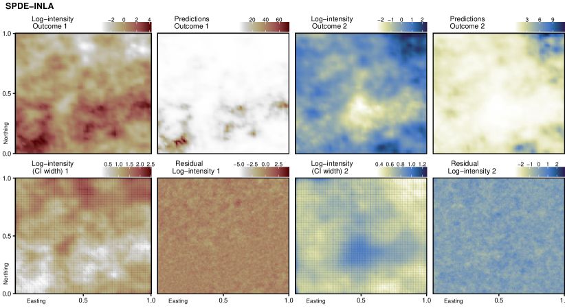
Figure 16: Output from fitting a SPDE model via INLA. Top row: recovered log-intensity and predictions for both outcomes. Bottom row: width of posterior credible intervals about log-intensity, and residual log-intensity.

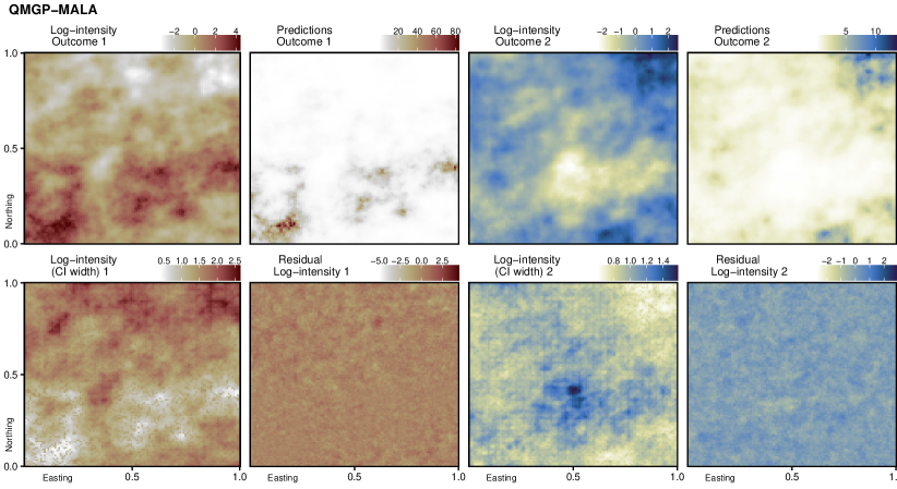
Figure 17: Output from fitting a coregionalized QMGP via MALA. Top row: recovered log-intensity and predictions for both outcomes. Bottom row: width of posterior credible intervals about log-intensity, and residual log-intensity.

E.2 Simulating 750 datasets with bivariate count outcomes

We provide additional details on the 750 simulated datasets of Figure 8 in the main article. We generate Poisson data on a $50\times 50$ regular grid, for a total of 2500 observations for $y_{j}(\boldsymbol{\ell})\sim Pois(\exp\{\eta_{j}(\boldsymbol{\ell})\})$ where $\boldsymbol{\eta}(\boldsymbol{\ell})=\boldsymbol{\Lambda}\boldsymbol{v}(\boldsymbol{\ell})$ and $\boldsymbol{v}(\cdot)$ is a bivariate GP with independent Matérn correlations with $\nu_{j}=1/2$ for $j=1,2$ and $\phi_{2}=2.5$. We choose $\phi_{1}\in\{2.5,12.5,25\}$. We introduce missing values at $1/5$ of spatial locations independently for each outcome. We fix the $2\times 2$ loading matrix via

$$\boldsymbol{\Lambda}=\begin{bmatrix}\lambda_{11}&\lambda_{12}\\ \lambda_{21}&\lambda_{22}\end{bmatrix}=\texttt{chol}\left(\begin{bmatrix}\lambda_{1}&0\\ 0&1\end{bmatrix}\cdot\begin{bmatrix}1&\rho\\ \rho&1\end{bmatrix}\cdot\begin{bmatrix}\lambda_{1}&0\\ 0&1\end{bmatrix}\right),$$

which implies $\lambda_{11}=\lambda_{1}$, $\lambda_{12}=0$, and $\lambda_{21}$ and $\lambda_{22}$ are such the latent correlation between the first and second margin is exactly $\rho$. We choose $\lambda_{1}\in\{\frac{\sqrt{2}}{2},2\}$ and $\rho\in\{-.9,-0.25,0,0.65,.9\}$. We generate 25 datasets for all combination of values of $\phi_{1}$, $\lambda_{1}$ and $\rho$. All QMGP models implemented in Section 5.1 use the GriPS method for sampling covariance parameters (Peruzzi et al., , 2021). Since the data are gridded, GriPS amounts to a parameter expansion strategy similar to the one used in Ghosh and Dunson, (2009). We report comparative results of the same analyses with/without GriPS in Figure 18. GriPS does not affect the relative performance of the tested methodologies for sampling QMGPs; however, it improves sampler efficiency and uncertainty quantification about the linear predictor. We note here that GriPS is less effective in higher dimensional multivariate cases and we did not observe advantages in the community ecology applications of Section 6 in the main article.

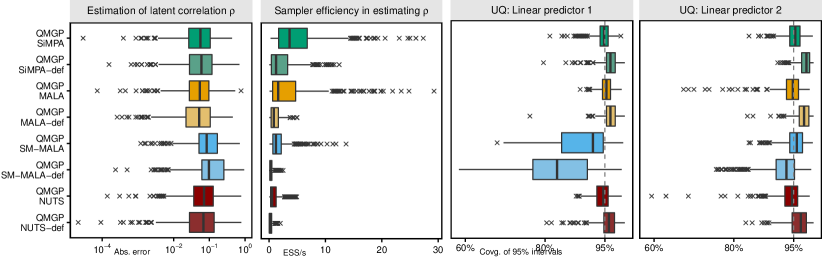
Figure 18: Estimation of $\rho$, its ESS/s, and coverage of intervals about $\eta_{j,\text{test}}$, with GriPS. Methods without GriPS are denoted as “-def”.

E.3 Latent process sampler efficiency in multi-type data

We use the same setup of Section E.2, choosing $\lambda_{1}\in\{2.5,12.5\}$, for each of the following pairs of outcome types: $\{(\text{Gaussian},\text{Poisson}),(\text{Neg. Binomial},\text{Binomial}),(\text{Neg. Binomial},\text{Poisson})\}$, for a total of 1500 datasets, of which 500 include a Binomial or Gaussian outcome, 1000 include a Poisson or Neg. Binomial outcome. We fix all unknowns ($\boldsymbol{\Lambda}$, $\phi_{1}$, $\phi_{2}$) to their true values except for the latent process, as we are interested in purely comparing sampling methods for $\boldsymbol{w}(\cdot)$. For each dataset, we calculate ESS/s for samples of $\boldsymbol{w}(\boldsymbol{\ell}_{i})$, $\boldsymbol{\ell}_{i}=1,\dots n$. After computing the median ESS/s as a summary efficiency measure for each dataset, we compute the mean of this measure over all datasets. Efficiency summary results are reported in Table 5. Comparisons based on RMSPE and coverage about $\eta_{j}(\boldsymbol{\ell}),j=1,2$ are in Table 6

Method	Binomial	Gaussian	Negative Binomial	Poisson
MALA	1.15	8.35	1.31	2.81
NUTS	0.25	2.15	0.32	0.68
SiMPA	4.26	17.65	9.03	8.90
SM-MALA	1.81	7.85	3.45	3.59

Table 5: Efficiency in posterior sampling of $\boldsymbol{w}(\cdot)$, in terms of ESS/s, for different types of outcome in the bivariate synthetic data application with multi-type outcomes.

Method	RMSPE				Covg. 95%
	Binomial	Gaussian	Neg. Bin.	Poisson	Binomial	Gaussian	Neg. Bin.	Poisson
MALA	0.450	0.332	14.206	1.198	0.897	0.942	0.899	0.930
NUTS	0.449	0.328	13.932	1.195	0.932	0.944	0.934	0.941
SiMPA	0.449	0.327	13.923	1.194	0.944	0.948	0.947	0.947
SM-MALA	0.449	0.327	13.971	1.212	0.943	0.948	0.939	0.940

Table 6: RMSPE in predicting the outcomes $\boldsymbol{y}_{j}(\boldsymbol{\ell})$ on the test set, and empirical coverage of 95% credible intervals about $\eta_{j}(\boldsymbol{\ell})$, $j=1,2$, for different types of outcome in the bivariate synthetic data application with multi-type outcomes.

References

• Andrieu and Thoms, (2008) Andrieu, C. and Thoms, J. (2008). A tutorial on adaptive MCMC. Statistics and Computing, 18:343–373. doi:10.1007/s11222-008-9110-y.
• Apanasovich and Genton, (2010) Apanasovich, T. V. and Genton, M. G. (2010). Cross-covariance functions for multivariate random fields based on latent dimensions. Biometrika, 97:15–30. doi:10.1093/biomet/asp078.
• Atchadé, (2006) Atchadé, Y. F. (2006). An adaptive version for the Metropolis adjusted Langevin algorithm with a truncated drift. Methodology and Computing in Applied Probability, 8:235–254. doi:10.1007/s11009-006-8550-0.
• Banerjee, (2017) Banerjee, S. (2017). High-dimensional Bayesian geostatistics. Bayesian Analysis, 12(2):583–614. doi:10.1214/17-BA1056R.
• Banerjee, (2020) Banerjee, S. (2020). Modeling massive spatial datasets using a conjugate Bayesian linear modeling framework. Spatial Statistics, 37:100417. doi:10.1016/j.spasta.2020.100417.
• Banerjee et al., (2010) Banerjee, S., Finley, A. O., Waldmann, P., and Ericsson, T. (2010). Hierarchical spatial process models for multiple traits in large genetic trials. Journal of American Statistical Association, 105(490):506–521. doi:10.1198/jasa.2009.ap09068.
• Banerjee et al., (2008) Banerjee, S., Gelfand, A. E., Finley, A. O., and Sang, H. (2008). Gaussian predictive process models for large spatial data sets. Journal of the Royal Statistical Society, Series B, 70:825–848. doi:10.1111/j.1467-9868.2008.00663.x.
• Betancourt, (2018) Betancourt, M. (2018). A conceptual introduction to Hamiltonian Monte Carlo. arXiv:1701.02434.
• Bhattacharya and Dunson, (2011) Bhattacharya, A. and Dunson, D. B. (2011). Sparse Bayesian infinite factor models. Biometrika, 98(2):291–306. doi:10.1093/biomet/asr013.
• Blomstedt et al., (2019) Blomstedt, P., Parente Paiva Mesquita, D., Lintusaari, J., Sivula, T., Corander, J., and Kaski, S. (2019). Meta-analysis of Bayesian analyses. arXiv:1904.04484.
• Bradley et al., (2018) Bradley, J. R., Holan, S. H., and Wikle, C. K. (2018). Computationally efficient multivariate spatio-temporal models for high-dimensional count-valued data (with discussion). Bayesian Analysis, 13(1):253–310. doi:10.1214/17-BA1069.
• Bradley et al., (2019) Bradley, J. R., Holan, S. H., and Wikle, C. K. (2019). Bayesian hierarchical models with conjugate full-conditional distributions for dependent data from the natural exponential family. Journal of the American Statistical Association. doi:10.1080/01621459.2019.1677471.
• Carpenter et al., (2017) Carpenter, B., Gelman, A., Hoffman, M. D., Lee, D., Goodrich, B., Betancourt, M., Brubaker, Marcus Guo, J., Li, P., and Riddell, A. (2017). Stan: A probabilistic programming language. Journal of Statistical Software, 76(1). doi:10.18637/jss.v076.i01.
• Chen et al., (2020) Chen, Z., Wang, B., and Gorban, A. N. (2020). Multivariate Gaussian and Student-t process regression for multi-output prediction. Neural Computing and Applications, 32:3005–3028. doi:10.1007/s00521-019-04687-8.
• Cressie and Johannesson, (2008) Cressie, N. and Johannesson, G. (2008). Fixed rank kriging for very large spatial data sets. Journal of the Royal Statistical Society, Series B, 70:209–226. doi:10.1111/j.1467-9868.2007.00633.x.
• Dagum and Menon, (1998) Dagum, L. and Menon, R. (1998). OpenMP: an industry standard api for shared-memory programming. Computational Science & Engineering, IEEE, 5(1):46–55.
• (17) Datta, A., Banerjee, S., Finley, A. O., and Gelfand, A. E. (2016a). Hierarchical nearest-neighbor Gaussian process models for large geostatistical datasets. Journal of the American Statistical Association, 111:800–812. doi:10.1080/01621459.2015.1044091.
• (18) Datta, A., Banerjee, S., Finley, A. O., Hamm, N. A. S., and Schaap, M. (2016b). Nonseparable dynamic nearest neighbor Gaussian process models for large spatio-temporal data with an application to particulate matter analysis. The Annals of Applied Statistics, 10:1286–1316. doi:10.1214/16-AOAS931.
• Dey et al., (2021) Dey, D., Datta, A., and Banerjee, S. (2021). Graphical Gaussian process models for highly multivariate spatial data. Biometrika. in press. doi:doi.org/10.1093/biomet/asab061.
• Duane et al., (1987) Duane, S., A.D., K., Pendleton, B. J., and Roweth, D. (1987). Hybrid Monte Carlo. Physics Letters B, 195:216–222.
• Dunson and Johndrow, (2020) Dunson, D. and Johndrow, J. E. (2020). The Hastings algorithm at fifty. Biometrika, 107(1):1–23. doi:10.1093/biomet/asz066.
• Finley et al., (2008) Finley, A. O., Banerjee, S., Ek, A. R., and McRoberts, R. E. (2008). Bayesian multivariate process modeling for prediction of forest attributes. Journal of Agricultural, Biological, and Environmental Statistics, 13:60. doi:10.1198/108571108X273160.
• Finley et al., (2019) Finley, A. O., Datta, A., Cook, B. D., Morton, D. C., Andersen, H. E., and Banerjee, S. (2019). Efficient algorithms for Bayesian nearest neighbor Gaussian processes. Journal of Computational and Graphical Statistics, 28:401–414. doi:10.1080/10618600.2018.1537924.
• Furrer et al., (2006) Furrer, R., Genton, M. G., and Nychka, D. (2006). Covariance tapering for interpolation of large spatial datasets. Journal of Computational and Graphical Statistics, 15:502–523. doi:10.1198/106186006X132178.
• Genton and Kleiber, (2015) Genton, M. G. and Kleiber, W. (2015). Cross-covariance functions for multivariate geostatistics. Statistical Science, 30:147–163. doi:10.1214/14-STS487.
• Ghosh and Dunson, (2009) Ghosh, J. and Dunson, D. B. (2009). Default prior distributions and efficient posterior computation in Bayesian factor analysis. Journal of Computational and Graphical Statistics, 18(2):306–320. doi:10.1198/jcgs.2009.07145.
• Girolami and Calderhead, (2011) Girolami, M. and Calderhead, B. (2011). Riemann manifold Langevin and Hamiltonian Monte Carlo methods. Journal of the Royal Statistical Society: Series B, 73(2):123–214. doi:10.1111/j.1467-9868.2010.00765.x.
• Gramacy and Apley, (2015) Gramacy, R. B. and Apley, D. W. (2015). Local Gaussian process approximation for large computer experiments. Journal of Computational and Graphical Statistics, 24(2):561–578. doi:10.1080/10618600.2014.914442.
• Guhaniyogi and Banerjee, (2018) Guhaniyogi, R. and Banerjee, S. (2018). Meta-kriging: Scalable Bayesian modeling and inference for massive spatial datasets. Technometrics, 60(4):430–444. doi:10.1080/00401706.2018.1437474.
• Haario et al., (2001) Haario, H., Saksman, E., and Tamminen, J. (2001). An adaptive Metropolis algorithm. Bernoulli, 7(2):223–242. doi:10.2307/3318737.
• Heaton et al., (2019) Heaton, M. J., Datta, A., Finley, A. O., Furrer, R., Guinness, J., Guhaniyogi, R., Gerber, F., Gramacy, R. B., Hammerling, D., Katzfuss, M., Lindgren, F., Nychka, D. W., Sun, F., and Zammit-Mangion, A. (2019). A case study competition among methods for analyzing large spatial data. Journal of Agricultural, Biological and Environmental Statistics, 24(3):398–425. doi:10.1007/s13253-018-00348-w.
• Hoffman and Gelman, (2014) Hoffman, M. D. and Gelman, A. (2014). The no-U-turn sampler: Adaptively setting path lengths in Hamiltonian Monte Carlo. Journal of Machine Learning Research, 15:351–1381.
• Jin et al., (2021) Jin, B., Peruzzi, M., and Dunson, D. B. (2021). Bag of DAGs: Flexible & scalable modeling of spatiotemporal dependence. arXiv:2112.11870.
• Johndrow et al., (2020) Johndrow, J. E., Pillai, N. S., and Smith, A. (2020). No free lunch for approximate mcmc. arXiv:2010.125147.
• Jönsson et al., (2010) Jönsson, A. M., Eklundh, L., Hellström, M., Bärring, L., and Jönsson, P. (2010). Annual changes in MODIS vegetation indices of Swedish coniferous forests in relation to snow dynamics and tree phenology. Remote Sensing of Environment, 114:2719–2730. doi:10.1016/j.rse.2010.06.005.
• Jurek and Katzfuss, (2020) Jurek, M. and Katzfuss, M. (2020). Hierarchical sparse Cholesky decomposition with applications to high-dimensional spatio-temporal filtering. arXiv:2006.16901.
• Katzfuss, (2017) Katzfuss, M. (2017). A multi-resolution approximation for massive spatial datasets. Journal of the American Statistical Association, 112:201–214. doi:10.1080/01621459.2015.1123632.
• Katzfuss and Guinness, (2021) Katzfuss, M. and Guinness, J. (2021). A general framework for Vecchia approximations of Gaussian processes. Statistical Science, 36(1):124–141. doi:10.1214/19-STS755.
• Kaufman et al., (2008) Kaufman, C. G., Schervish, M. J., and Nychka, D. W. (2008). Covariance tapering for likelihood-based estimation in large spatial data sets. Journal of the American Statistical Association, 103:1545–1555. doi:10.1198/016214508000000959.
• Lindgren et al., (2011) Lindgren, F., Rue, H., and Lindström, J. (2011). An explicit link between Gaussian fields and Gaussian Markov random fields: the stochastic partial differential equation approach. Journal of the Royal Statistical Society: Series B, 73:423–498. doi:10.1111/j.1467-9868.2011.00777.x.
• Marshall and Roberts, (2012) Marshall, T. and Roberts, G. (2012). An adaptive approach to Langevin MCMC. Statistics and Computing, 22:1041–1057. doi:10.1007/s11222-011-9276-6.
• Matheron, (1982) Matheron, G. (1982). Pour une analyse krigeante des données régionalisées. Technical report N.732, Centre de Géostatistique.
• Mesquita et al., (2020) Mesquita, D., Blomstedt, P., and Kaski, S. (2020). Embarrassingly parallel MCMC using deep invertible transformations. In Adams, R. P. and Gogate, V., editors, Proceedings of Machine Learning Research, volume 115, pages 1244–1252, Tel Aviv, Israel. PMLR. http://proceedings.mlr.press/v115/mesquita20a.html.
• Neal, (2011) Neal, R. M. (2011). MCMC using Hamiltonian dynamics. In Brooks, S., Gelman, A., Jones, G. L., and Meng, X.-L., editors, Handbook of Markov Chain Monte Carlo. CRC Press, New York. doi:10.1201/b10905.
• Neiswanger et al., (2014) Neiswanger, W., Wang, C., and Xing, E. P. (2014). Asymptotically exact, embarrassingly parallel MCMC. In Proceedings of the Thirtieth Conference on Uncertainty in Artificial Intelligence, UAI’14, page 623–632, Arlington, Virginia, USA. AUAI Press.
• Nemeth and Sherlock, (2018) Nemeth, C. and Sherlock, C. (2018). Merging mcmc subposteriors through gaussian-process approximations. Bayesian Analysis, 13(2):507–530. doi:doi = "10.1214/17-BA1063".
• Peruzzi et al., (2021) Peruzzi, M., Banerjee, S., Dunson, D. B., and Finley, A. O. (2021). Grid-Parametrize-Split (GriPS) for improved scalable inference in spatial big data analysis. arXiv:2101.03579.
• Peruzzi et al., (2020) Peruzzi, M., Banerjee, S., and Finley, A. O. (2020). Highly scalable Bayesian geostatistical modeling via meshed Gaussian processes on partitioned domains. Journal of the American Statistical Association. in press. doi:10.1080/01621459.2020.1833889.
• Peruzzi and Dunson, (2021) Peruzzi, M. and Dunson, D. B. (2021). Spatial multivariate trees for big data Bayesian regression. Journal of Machine Learning Research, accepted. arXiv:2012.00943.
• Roberts and Rosenthal, (2007) Roberts, G. O. and Rosenthal, J. S. (2007). Coupling and ergodicity of adaptive Markov chain Monte Carlo algorithms. Journal of Applied Probability, 44:458–475. doi:10.1239/jap/1183667414.
• Roberts and Stramer, (2002) Roberts, G. O. and Stramer, O. (2002). Langevin diffusions and Metropolis-Hastings algorithms. Methodology And Computing In Applied Probability, 4:337–357. doi:10.1023/A:1023562417138.
• Roberts and Tweedie, (1996) Roberts, G. O. and Tweedie, R. L. (1996). Exponential convergence of Langevin distributions and their discrete approximations. Bernoulli, 2(4):341–363.
• Rue and Held, (2005) Rue, H. and Held, L. (2005). Gaussian Markov Random Fields: Theory and Applications. Chapman & Hall/CRC. doi:10.1007/978-3-642-20192-9.
• Rue et al., (2009) Rue, H., Martino, S., and Chopin, N. (2009). Approximate Bayesian inference for latent Gaussian models by using integrated nested laplace approximations. Journal of the Royal Statistical Society: Series B, 71:319–392. doi:10.1111/j.1467-9868.2008.00700.x.
• Sang and Huang, (2012) Sang, H. and Huang, J. Z. (2012). A full scale approximation of covariance functions for large spatial data sets. Journal of the Royal Statistical Society, Series B, 74:111–132. doi:10.1111/j.1467-9868.2011.01007.x.
• Schmidt and Gelfand, (2003) Schmidt, A. M. and Gelfand, A. E. (2003). A Bayesian coregionalization approach for multivariate pollutant data. Journal of Geophysical Research, 108:D24. doi:10.1029/2002JD002905.
• Sengupta and Cressie, (2013) Sengupta, A. and Cressie, N. (2013). Hierarchical statistical modeling of big spatial datasets using the exponential family of distributions. Spatial Statistics. doi:10.1016/j.spasta.2013.02.002.
• Shah et al., (2014) Shah, A., Wilson, A. G., and Ghahramani, Z. (2014). Student-t processes as alternatives to Gaussian processes. In Proceedings of the 17th International Conference on Artificial Intelligence and Statistics (AISTATS).
• Shirota et al., (2019) Shirota, S., Finley, A. O., Cook, B. D., and Banerjee, S. (2019). Conjugate nearest neighbor Gaussian process models for efficient statistical interpolation of large spatial data. arXiv:1907.10109.
• Stein, (2014) Stein, M. L. (2014). Limitations on low rank approximations for covariance matrices of spatial data. Spatial Statistics, 8:1–19. doi:doi:10.1016/j.spasta.2013.06.003.
• Stein et al., (2004) Stein, M. L., Chi, Z., and Welty, L. J. (2004). Approximating likelihoods for large spatial data sets. Journal of the Royal Statistical Society, Series B, 66:275–296. doi:10.1046/j.1369-7412.2003.05512.x.
• Sun et al., (2011) Sun, Y., Li, B., and Genton, M. (2011). Geostatistics for large datasets. In Montero, J., Porcu, E., and Schlather, M., editors, Advances and Challenges in Space-time Modelling of Natural Events, pages 55–77. Springer-Verlag, Berlin Heidelberg. doi:10.1007/978-3-642-17086-7.
• Taylor and Diggle, (2014) Taylor, B. M. and Diggle, P. J. (2014). INLA or MCMC? a tutorial and comparative evaluation for spatial prediction in log-Gaussian Cox processes. Journal of Statistical Computation and Simulation, 84(10):2266–2284. doi:10.1080/00949655.2013.788653.
• Tikhonov et al., (2020) Tikhonov, G., Opedal, O. H., Abrego, N., Lehikoinen, A., de Jonge, M. M. J., Oksanen, J., and Ovaskainen, O. (2020). Joint species distribution modelling with the R-package Hmsc. Methods in Ecology and Evolution, 11(3):442–447. doi:10.1111/2041-210X.13345.
• Vecchia, (1988) Vecchia, A. V. (1988). Estimation and model identification for continuous spatial processes. Journal of the Royal Statistical Society, Series B, 50:297–312. doi:10.1111/j.2517-6161.1988.tb01729.x.
• Vihola, (2012) Vihola, M. (2012). Robust adaptive Metropolis algorithm with coerced acceptance rate. Statistics and Computing, 22:997–1008. doi:10.1007/s11222-011-9269-5.
• Wackernagel, (2003) Wackernagel, H. (2003). Multivariate Geostatistics: An Introduction with Applications. Springer, Berlin. doi:10.1007/978-3-662-05294-5.
• Walker et al., (1993) Walker, D. A., Halfpenny, J. C., Walker, M. D., and Wessman, C. A. (1993). Long-term studies of snow-vegetation interactions. BioScience, 43(5):287–301. doi:10.2307/1312061.
• (69) Wang, K., Zhang, L., Qiu, Y., Ji, L., Tian, F., Wang, C., and Wang, Z. (2015a). Snow effects on alpine vegetation in the Qinghai-Tibetan plateau. International Journal of Digital Earth, 8(1):58–75. doi:10.1080/17538947.2013.848946.
• Wang and Dunson, (2014) Wang, X. and Dunson, D. B. (2014). Parallelizing MCMC via Weierstrass sampler. arXiv:1312.4605.
• (71) Wang, X., Guo, F., Heller, K. A., and Dunson, D. B. (2015b). Parallelizing MCMC with random partition trees. In Proceedings of the 28th International Conference on Neural Information Processing Systems - Volume 1, NIPS’15, page 451–459, Cambridge, MA, USA. MIT Press. arXiv:1506.03164.
• Xie et al., (2020) Xie, J., Jonas, T., Rixen, C., de Jong, R., Garonna, I., Notarnicola, C., Asam, S., Schaepman, M. E., and Kneubühler, M. (2020). Land surface phenology and greenness in Alpine grasslands driven by seasonal snow and meteorological factors. Science of The Total Environment, 725:138380. doi:10.1016/j.scitotenv.2020.138380.
• Zanella and Roberts, (2021) Zanella, G. and Roberts, G. (2021). Multilevel linear models, gibbs samplers and multigrid decompositions. Bayesian Analysis. doi:10.1214/20-BA1242.
• Zhang and Banerjee, (2021) Zhang, L. and Banerjee, S. (2021). Spatial factor modeling: A Bayesian matrix-normal approach for misaligned data. Biometrics. doi:10.1111/biom.13452.
• Zilber and Katzfuss, (2020) Zilber, D. and Katzfuss, M. (2020). Vecchia-Laplace approximations of generalized Gaussian processes for big non-Gaussian spatial data. arXiv:1906.07828.