A First Look at First-Passage Processes

Abstract

These notes are based on the lectures that I gave (virtually) at the Bruneck Summer School in 2021 on first-passage processes and some applications of the basic theory. I begin by defining a first-passage process and presenting the connection between the first-passage probability and the familiar occupation probability. Some basic features of first passage on the semi-infinite line and a finite interval are then discussed, such as splitting probabilities and first-passage times. I also treat the fundamental connection between first passage and electrostatics. A number of applications of first-passage processes are then presented, including the hitting probability for a sphere in greater than two dimensions, reaction rate theory and its extension to receptors on a cell surface, first-passage inside an infinite absorbing wedge in two dimensions, stochastic hunting processes in one dimension, the survival of a diffusing particle in an expanding interval, and finally the dynamics of the classic birth-death process.

1 What is a First-Passage Process?

The first-passage probability is defined as the probability that a diffusing particle or a random walk first reaches a given site (or set of sites) at a specified time. Typical examples of first-passage processes include: fluorescence quenching, in which light emission by a fluorescent molecule stops when it reacts with a quencher; integrate-and-fire neurons, in which a neuron fires when a fluctuating voltage level first reaches a specified level; and the execution of buy/sell orders when a stock price first reaches a threshold. To appreciate why first-passage phenomena might be relevant practically, consider the following example. You are an investor who buys stock in a company at a price of $100. Suppose that this price fluctuates daily by $\pm\$1$. You will sell if the stock price reaches $200 and if the stock price reaches $0, the company has gone bankrupt and you’ve lost all your investment. What it the probability of doubling your investment or losing your entire investment? How long will it take before one of these two events occurs? These are the types of questions that are the purview of first-passage phenomena. Much of the material covered here is discussed more detail in this monograph [1], and in other general reviews and texts on probability theory and stochastic processes [2, 3, 4, 5].

2 First-Passage and Occupation Probabilities

Let’s start by deriving the formal relation between the first-passage probability and the familiar occupation probability. For concreteness, consider a random walk in discrete space and discrete time. We define $P(\mathbf{r},t)$ as the occupation probability; this is the probability that a random walk is at site $\mathbf{r}$ at time $t$ when it starts at the origin. Similarly, let $F(\mathbf{r},t)$ be the first-passage probability, namely, the probability that the random walk first visits $\mathbf{r}$ at time $t$ with the same initial condition. Clearly $F(\mathbf{r},t)$ decays more rapidly in time than $P(\mathbf{r},t)$ because once a random walk reaches $\mathbf{r}$, there can be no further contribution to $F(\mathbf{r},t)$, although the same walk may still contribute to $P(\mathbf{r},t)$.

Figure 1: Schematic diagrammatic relation between the occupation probability of a random walk (whose propagation is represented by a wavy line) and the first-passage probability (straight line).

It is convenient to write $P(\mathbf{r},t)$ in terms of $F(\mathbf{r},t)$ and then invert this relation to find $F(\mathbf{r},t)$. For a random walk to be located at $\mathbf{r}$ at time $t$, the walk must first reach $\mathbf{r}$ at some earlier time step $t^{\prime}$ and then return to $\mathbf{r}$ after $t-t^{\prime}$ additional steps (Fig. 1). This connection between $F(\mathbf{r},t)$ and $P(\mathbf{r},t)$ may be expressed as the convolution

$$P(\mathbf{r},t)=\delta_{\mathbf{r},0}\delta_{t,0}+\sum_{t^{\prime}\leq t}F(\mathbf{r},t^{\prime})\,P(0,t-t^{\prime})\,,$$ (2.1)

where $\delta_{t,0}$ is the Kronecker delta function. This equation expresses the fact that if a random walk is at $\mathbf{r}$ at time $t$, it must have first reached $\mathbf{r}$ at some earlier time $t^{\prime}$ (which could even be $t$). If the walk reached $\mathbf{r}$ at a time earlier than $t$, then it must return to $\mathbf{r}$ (and any number of such returns could occur) in the remaining time $t-t^{\prime}$. The probability for this set of events is expressed by $P(0,t-t^{\prime})$. The delta function term accounts for the initial condition that the walk starts at $\mathbf{r}=0$.

The above convolution is most conveniently solved by introducing the generating functions,

$$P(\mathbf{r},z)=\sum_{t=0}^{\infty}P(\mathbf{r},t)z^{t}\,,\qquad F(\mathbf{r},z)=\sum_{t=0}^{\infty}F(\mathbf{r},t)z^{t}\,.$$

For a random walk in continuous time, we would merely replace the sum over discrete time in Eq. (2.1) by an integral and then use the Laplace transform. However, the asymptotic results would be identical. To solve for the first-passage probability, we multiply Eq. (2.1) by $z^{t}$ and sum over all $t$. We thereby find that the generating functions for $P$ and $F$ are related by

$$P(\mathbf{r},z)=\delta_{\mathbf{r},0}+F(\mathbf{r},z)P(0,z)\,.$$ (2.2)

Thus we obtain the fundamental connection between the generating functions

$$F(\mathbf{r},z)=\begin{cases}{\displaystyle\frac{P(\mathbf{r},z)}{P(0,z)}}&\mathbf{r}\neq 0\,,\\[11.38109pt] {\displaystyle 1-\frac{1}{P(0,z)}},&\mathbf{r}=0\,.\end{cases}$$ (2.3)

The important point is that the first-passage probability can be determined solely from the occupation probability. Many profound results about random walks in infinite space can be obtained from the fundamental relation (2.3) (see, e.g., [6, 7, 8, 9]). Our focus here will be on random walks or diffusion in confined geometries that reflect important physical constraints.

3 The Half Line

Suppose that a diffusing particle starts at $x_{0}>0$ on the infinite half line $[0,\infty]$ and is absorbed when it reaches the origin. Does the particle ever reach the origin? If so, when does this particle first reach the origin? To answer these questions, we have to solve the diffusion equation for the concentration $c(x,t)$, subject to the initial condition $c(x,t\!=\!0)=\delta(x-x_{0})$, and the boundary condition $c(x\!=\!0,t\!>\!0)=0$; the latter enforces the absorption of the particle when it reaches the origin.

A standard approach to solve this problem is to first take the Laplace transform of the diffusion equation and then solve for the Green’s function of this transformed equation. Then one inverts the Laplace transform of the Green’s function to obtain the concentration $c(x,t)$ in the time domain. The diffusive flux to the origin gives the probability that the particle reaches the origin at time $t$. Because of the absorbing boundary condition, when the particle does reach the origin, it is removed from the system. Thus the diffusive flux corresponds to the probability for the particle to reach the origin for the first time—namely, the first-passage probability to the origin.

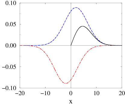
Figure 2: Concentration profile of a diffusing particle on the absorbing infinite half line $(0,\infty)$ at $Dt=10$, with $x_{0}=2$ (solid curve). Also shown are the component Gaussian (blue dashed) and image anti-Gaussian (red dot-dash) and their superposition in the physical region $x>0$.

A more fun way to solve this problem is by invoking the familiar image method from electrostatics. In this method, a diffusing particle that starts at $x_{0}>0$ and is subject to an absorbing boundary condition at $x=0$ is equivalent to removing the boundary altogether and introducing an image “antiparticle” that is initially at $x=-x_{0}$. Because the concentration is clearly equal to zero at the origin by symmetry, this image antiparticle effectively imposes the absorbing boundary condition $c(x\!=\!0,t)=0$. The initial particle and the image antiparticle both diffuse freely on $[-\infty,\infty]$ and their superposition gives a resultant concentration $c(x,t)$ for $x>0$ that solves the original problem.

Hence the concentration for a diffusing particle on the positive half-line is the sum of a Gaussian centered at $x_{0}$ and an anti-Gaussian centered at $-x_{0}$:

$$c(x,t)=\frac{1}{\sqrt{4\pi Dt}}\left[e^{-(x-x_{0})^{2}/4Dt}-e^{-(x+x_{0})^{2}/4Dt}\right].$$ (3.1)

This concentration profile has a linear dependence on $x$ near the origin and a Gaussian tail for $x/\sqrt{Dt}\gg 1$, as illustrated in Fig. 2. Because the initial condition is normalized, the first-passage probability to the origin at time $t$ is just the diffusive flux to this point. From the above expression for $c(x,t)$, we find

$$F(0,t)=+D\frac{\partial c(x,t)}{\partial x}\bigg{|}_{x=0}=\frac{x_{0}}{\sqrt{4\pi Dt^{3}}}\,\,e^{-x_{0}^{2}/4Dt}\qquad t\to\infty\,.$$ (3.2)

This fundamental and simple formula has a number of striking implications:

1. The particle is sure to reach to the origin because $\int_{0}^{\infty}F(0,t)\,dt=1$. That is, eventual absorption is certain.

2. The average time for the particle to reach the origin is infinite! This fact arises because the first-passage probability has the long-time algebraic tail $F(0,t)\to x_{0}/\sqrt{4\pi Dt^{3}}$ for $t\gg x_{0}^{2}/D$. This dichotomy between hitting the origin with certainty but taking an infinite average time to do so underlies many of the intriguing features of one-dimensional diffusion.

3. The typical time to reach the origin is finite. We can define the term typical time in a precise way as follows: As a preliminary, define the typical position of the particle, $x_{T}$, as

   $$\int_{x_{T}}^{\infty}c(x,t)\,dx=\tfrac{1}{2}\,.$$ (3.3)

   That is, one half of the total probability lies in the range beyond $x_{T}$ and one half lies in the range $[0,x_{T}]$. Substituting the concentration profile (3.1) into the above integral and performing the integral leads to the transcendental equation

   $$\text{erfc}\left(\frac{x_{T}-x_{0}}{\sqrt{4Dt}}\right)-\text{erfc}\left(\frac{x_{T}+x_{0}}{\sqrt{4Dt}}\right)=1\,.$$ (3.4)

   This equation can only be solved numerically and the salient feature is that $x_{T}$ monotonically decreases with time and reaches zero at a time that is roughly $1.1\,x_{0}^{2}/D$; this defines the typical hitting time.

4. Even though the average time to reach the origin is infinite, the number of times the origin is reached in a time $t$ is proportional to $\sqrt{t}$. This result follows directly from the probability distribution of a freely diffusing particle. At large times, the bulk of Gaussian distribution for a particle that starts at $x_{0}$ will spread past the origin. Each site that is within the Gaussian envelope will have been visited of the order of $\sqrt{t}$ times. This last fact will be relevant for our discussion of the reaction rate of the sphere in Sec. 6.

4 The Finite Interval

We now turn to the first-passage properties in a finite interval. The reason for focusing on the finite interval is that the basic first-passage questions in this geometry have many profound implications. Moreover, the interval geometry is sufficiently simple that many results can be readily derived. Let us begin by outlining the basic questions that we will address. We consider a diffusing particle that starts at some point $x_{0}$ within the interval $[0,L]$, with absorbing boundary conditions at both ends of the interval. Eventually the particle is absorbed, and our goal is to characterize the time dependence of this absorption. Basic first-passage questions include:

1. What is the time dependence of the survival probability $S(t)$? This is the probability that a diffusing particle does not touch either absorbing boundary before time $t$.

2. What is the time dependence of the first-passage, or exit probabilities, to either 0 or to $L$ as a function of $x_{0}$? Integrating these probabilities over all time gives the eventual hitting, or splitting probability to a specified boundary. What is the dependence of the splitting probability to 0 or to $L$ as a function of the starting position?

3. What is the average exit time, that is, the average time until the particle hits either of the absorbing boundaries as a function of starting position? What are the conditional exit times, that is, the average time to hit a specified boundary (without ever touching the other boundary) as a function of the starting position?

To answer the first question, we need to solve the diffusion equation in the interval, subject to the initial condition that a particle starts at $x_{0}$, and with absorbing boundary conditions at both ends. This is a standard exercise and the result for the concentration is

$$c(x,t)=\sum_{n\geq 1}^{\infty}\frac{2}{L}\sin\frac{n\pi x_{0}}{L}\,\sin\frac{n\pi x}{L}\;e^{-n^{2}\pi^{2}\,Dt/L^{2}}~{}.$$ (4.1)

Since the large-$n$ eigenmodes decay more rapidly in time, the most slowly decaying eigenmode dominates in the long-time limit. As a result, the survival probability, which is the spatial integral of the concentration over the interval, asymptotically decays as

$$S(t)\sim e^{-D\pi^{2}t/L^{2}}\,.$$ (4.2)

For answering the second question, it is mathematically simpler to work in the Laplace transform domain. Applying the Laplace transform to the diffusion equation recasts it as

$$sc(x,s)-c(x,t=0)=Dc^{\prime\prime}(x,s)\,,$$ (4.3)

where the prime denotes differentiation with respect to $x$. The argument $s$ indicates that $c(x,s)$ is the Laplace transform. Within the standard Green’s function approach, the homogeneous equation in each subdomain $(0,x_{0})$ and $(x_{0},L)$ has elementary solutions of the form $c(x,s)=A\exp(x\sqrt{{s/D}})+B\exp(-x\sqrt{{s/D}})$, with the constants $A$ and $B$ determined by the boundary conditions. Because the absorbing boundary condition at $x=0$ mandates an antisymmetric combination of exponentials and because the form of the Green’s function as $x\to L$ must be identical to that as $x\to 0$, we can be immediately write

$$\begin{split}c_{<}(x,s)&=A\sinh\left(\sqrt{\frac{s}{D}}\,x\right)\hskip 36.135ptx<x_{0}\,,\\[5.69054pt] c_{>}(x,s)&=B\sinh\left(\sqrt{\frac{s}{D}}(L-x)\right)\quad x>x_{0}\,,\end{split}$$ (4.4)

for the subdomain Green’s functions $c_{<}$ and $c_{>}$, where $A$ and $B$ are constants.

We now impose the continuity condition $c_{<}(x_{0},s)=c_{>}(x_{0},s)$ and the jump condition that is obtained by integrating Eq. (4.3) over an infinitesimal interval that includes $x_{0}$:

$$c^{\prime}(x,s)\big{|}_{x=x_{0}^{+}}-c^{\prime}(x,s)\big{|}_{x=x_{0}^{-}}=-1/D\,,$$

to finally obtain

$$c(x,s)=\frac{\displaystyle\sinh\left(\sqrt{\frac{s}{D}}\,x_{<}\right)\sinh\left(\sqrt{\frac{s}{D}}(L-x_{>})\right)}{\displaystyle\sqrt{sD}\sinh\left(\sqrt{\frac{s}{D}}\,L\right)}\,.$$ (4.5)

From this Green’s function, the Laplace transform of the fluxes at $x=0$ and at $x=L$ are

$$j_{-}(s|x_{0}) \equiv+D\frac{\partial c(x,s)}{\partial x}\Bigg{|}_{x=0}={\displaystyle\sinh\left({\sqrt{\frac{s}{D}}}(L-x_{0})\right)}\bigg{/}{\displaystyle\sinh\left({\sqrt{\frac{s}{D}}}\,L\right)}\,.$$ (4.6a)

$$j_{+}(s|x_{0}) \equiv-D\frac{\partial c(x,s)}{\partial x}\Bigg{|}_{x=L}={\displaystyle\sinh\left(\sqrt{\frac{s}{D}}\,x_{0}\right)}\bigg{/}{\displaystyle\sinh\left(\sqrt{\frac{s}{D}}\,L\right)}\,.$$ (4.6b)

The subsidiary argument $x_{0}$ in $j$ emphasizes that the flux depends on the initial particle position. Since the initial condition is normalized, the magnitude of the flux to each boundary is identical to the respective first-passage probabilities.

For $s=0$, these Laplace transforms are just the time-integrated first-passage probabilities to 0 and at $L$. These quantities therefore coincide with the respective splitting probabilities, ${\mathcal{E}}_{-}(x_{0})$ and ${\mathcal{E}}_{+}(x_{0})$, namely, the probabilities to eventually hit the left and the right ends of the interval as a function of the initial position $x_{0}$:

$$\begin{split}{\mathcal{E}}_{-}(x_{0})&=j_{-}(s\!=\!0|x_{0})=1-\frac{x_{0}}{L}\,,\\[5.69054pt] {\mathcal{E}}_{+}(x_{0})&=j_{+}(s\!=\!0|x_{0})=\frac{x_{0}}{L}\,.\end{split}$$ (4.7)

Thus the splitting probabilities are given by an amazingly simple formula—the probability of reaching one endpoint is just the fractional distance to the other endpoint!

It is instructive to also derive these splitting probabilities by the backward Kolmogorov approach [1, 2]. The word backward reflects the feature that the initial condition becomes the dependent variable, rather than the current position of the particle. As we shall see, this method provides a powerful tool for determining first-passage properties. Physically, we obtain the eventual hitting probability ${\mathcal{E}}_{+}(x_{0})$ to the right boundary by summing the probabilities for all paths that start at $x_{0}$ and reach $L$ without touching $0$. Thus

$${\mathcal{E}}_{+}(x_{0})=\sum_{\text{paths}}\Pi_{x_{0}\to L}\,,$$ (4.8)

where $\Pi_{x_{0}\to L}$ denotes the probability of a path from $x_{0}$ to $L$ that avoids $0$. As illustrated in Fig. 3, the sum over all such paths can be decomposed into the outcome after one step and the sum over all path remainders from the intermediate point $x^{\prime}$ to $L$. This gives

$$\mathcal{E}_{+}(x_{0})=\tfrac{1}{2}\sum_{\text{paths}^{\prime}}\Pi_{x_{0}+\delta x\to L}+\tfrac{1}{2}\,\sum_{\text{paths}^{\prime\prime}}\Pi_{x_{0}-\delta x\to L}=\tfrac{1}{2}[{\mathcal{E}}_{+}(x_{0}\!+\!\delta x)+{\mathcal{E}}_{+}(x_{0}\!-\!\delta x)]\,.$$ (4.9)

Here $\delta x$ is the length of a single random-walk step and paths^′ and paths^′′ indicate, respectively, all paths that start at $x_{0}\pm\delta x$ and reach $L$ without touching 0.

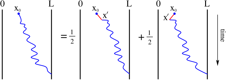
Figure 3: Schematic decomposition of a random walk path from $x_{0}$ to $L$ into the outcome after one step (red) and the remainder from $x^{\prime}$ to $L$. The factors $1/2$ account for the probabilities associated with the first step of the decomposed paths.

Equation (4.9) reduces to $\Delta^{(2)}{\mathcal{E}}_{\pm}(x_{0})=0$, where $\Delta^{(2)}$ is the discrete second-difference operator, $\Delta^{(2)}f(x)\equiv f(x-\delta x)-2f(x)+f(x+\delta x)$. This difference equation is subject to the boundary conditions ${\mathcal{E}}_{+}(0)=0$, ${\mathcal{E}}_{+}(L)=1$. The solution is simply

$${\mathcal{E}}_{+}(x_{0})=\frac{x}{L}\,,$$ (4.10)

and correspondingly ${\mathcal{E}}_{-}(x)=1-\frac{x}{L}$.

It is worth mentioning that there is an even simpler way to determine the exit probabilities by the martingale method [10]. This solution relies on the fact that the motion of the random walk in the interval is a “fair game” at any time. Thus the average position of the walk is time independent. Formally, a martingale is a process in which the average value of a random variable at time $t+\delta t$ equals the average value of this variable at time $t$.

For the present example, at $t=0$, the average position of the particle is $\langle x\rangle=x_{0}$. At infinite time, the walk is either at the left end or the right end of the interval, with respective probabilities ${\mathcal{E}}_{+}(x_{0})$ or ${\mathcal{E}}_{-}(x_{0})$. Thus the average position at infinite time is $\langle x\rangle=0\times{\mathcal{E}}_{-}(x_{0})+L\times{\mathcal{E}}_{+}(x_{0})$. Since the initial average position equals the final average position, we immediately recover (4.10).

For a biased random walk with a probability $p$ of hopping to the right and probability $q$ of hopping to the left, the analog of Eq. (4.9) for the splitting probability is

$${\mathcal{E}}(x_{0})=p{\mathcal{E}}_{+}(x_{0}\!+\!\delta x)+q{\mathcal{E}}_{+}(x_{0}\!-\!\delta x)\,,$$ (4.11)

with solution

$${\mathcal{E}}_{+}(x_{0})=\frac{1-e^{-vx_{0}/D}}{1-e^{-vL/D}}\equiv\frac{1-e^{-u_{0}P\!e}}{1-e^{-P\!e}}\,,$$ (4.12)

where $v=(p-q)\delta x$, $D=\delta x^{2}/2$, $u_{0}=x_{0}/L$, and $P\!e=vL/D$ is the Péclet number, which is a dimensionless measure of the influence of the bias relative to diffusive fluctuations. When the Péclet number is large, the exit probability clearly reflects the strong influence of the bias (Fig. 4).

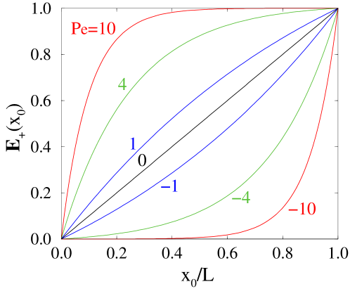
Figure 4: Dependence of the exit probability to $x=L$ on $u_{0}=x_{0}/L$ in the interval $[0,L]$ for various Péclet numbers $P\!e$.

We now extend the backward Kolmogorov approach to determine the average exit time from the finite interval. We distinguish between the unconditional average exit time, namely, the average time for a particle to reach either end of the interval, and the conditional average exit time, namely, the average time for a particle to reach, say, the right end of the interval without ever touching the other end.

In close analogy with (4.8), the unconditional exit time satisfies

$$t(x_{0})=\sum_{\text{paths}}(\Pi t)_{x_{0}\to\pm L}\,.$$ (4.13)

That is, to compute the average unconditional exit time, we take the time for a path to go from $x_{0}$ to $\pm L$ times the probability of this path and sum over all possible paths. Using the same decomposition that which led to (4.9), the unconditional exit time satisfies

$$t(x_{0}) =\tfrac{1}{2}\!\!\sum_{\text{paths}^{\prime}}\!\!\Pi_{x_{0}+\delta x\to\pm L}(t_{x_{0}+dx\to\pm L}\!+\!dt)+\tfrac{1}{2}\!\!\sum_{\text{paths}^{\prime\prime}}\!\!\Pi_{x_{0}-\delta x\to\pm L}(t_{x_{0}-dx\to\pm L}\!+\!dt)\,.$$ (4.14)

Notice that the term

$$\tfrac{1}{2}\!\!\sum_{\text{paths}^{\prime}}\!\!\Pi_{x_{0}+\delta x\to\pm L}\;t_{x_{0}+dx\to\pm L}$$

has exactly the same form as (4.13), so that the above expression is merely $\frac{1}{2}t(x_{0}+\delta x)$. A similar identification holds for the analogous term

$$\tfrac{1}{2}\!\!\sum_{\text{paths}^{\prime\prime}}\!\!\Pi_{x_{0}-\delta x\to\pm L}\;t_{x_{0}-dx\to\pm L}\,.$$

Finally, the terms multiplying the factor $dt$ in (4.14) just gives the probability of all possible paths from $x_{0}$ to either end of the interval; this probability is clearly equal to 1. Thus we have

$$t(x_{0})=\tfrac{1}{2}[t(x_{0}\!+\!\delta x)+t(x_{0}\!-\!\delta x)]+dt\,.$$ (4.15)

In the continuum limit, we expand (4.15) in a Taylor series to second order in $\delta x$ to give

$$\frac{\delta x^{2}}{2}t^{\prime\prime}=-dt\,.$$

Now identifying $\delta x^{2}/(2dt)$ as the diffusion coefficient $D$, the equation for the unconditional exit time reduces to $D\,t^{\prime\prime}=-1$, subject to the boundary conditions $t(0)=t(L)=0$. The solution is (see Fig. 5)

$$t(x_{0})=\frac{x_{0}(L-x_{0})}{2D}\,.$$ (4.16)

Notice that this exit time is of the order of $L$ for a particle that starts a distance of the order of one from an absorbing boundary and of the order of $L^{2}$ for a particle that starts near the middle of the interval.

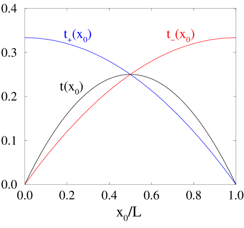
Figure 5: Unconditional and conditional average exit times from the finite interval $[0,L]$, normalized by $L^{2}/2D$, as a function of the dimensionless initial position $x_{0}/L$.

Now let’s calculate the conditional exit time to the right boundary when starting from $x_{0}$, $t_{+}(x_{0})$. By definition this conditional time is

$$t_{+}(x_{0})=\frac{\sum_{\text{paths}_{+}}(\Pi t)_{x_{0}\to L}}{\sum_{\text{paths}_{+}}\Pi_{x_{0}\to L}}=\frac{\sum_{\text{paths}_{+}}(\Pi t)_{x_{0}\to L}}{{\mathcal{E}}_{+}(x_{0})}\,.$$ (4.17)

That is, the conditional exit time is the time for a path to start at $x_{0}$ and reach $L$ without touching 0 multiplies by the probability of this path, summed over all such allowable paths. Here the subscript + on the word paths indicates that only paths that go from $x_{0}$ to $L$ without touching 0 are included. Since the total probability of all these restricted paths is less than 1, we need to divide by this total probability, ${\mathcal{E}}_{+}(x_{0})$, to obtain the properly normalized conditional exit time. Thus, for the quantity ${\mathcal{E}}_{+}(x_{0})t_{+}(x_{0})$, we have

$${\mathcal{E}}_{+}(x_{0})t_{+}(x_{0}) =\sum_{\text{paths}_{+}}(\Pi t)_{x_{0}\to L}$$

$$=\tfrac{1}{2}\!\!\sum_{\text{paths}^{\prime}_{+}}\Pi(t_{x_{0}+dx\to L}+dt)+\tfrac{1}{2}\!\!\sum_{\text{paths}^{\prime\prime}_{+}}\Pi(t_{x_{0}-dx\to L}+dt)$$

$$=\tfrac{1}{2}\left[{\mathcal{E}}_{+}(x_{0}\!+\!dx)t_{+}(x_{0}\!+\!dx)\right]+\tfrac{1}{2}\left[{\mathcal{E}}_{+}(x_{0}\!-\!dx)t_{+}(x_{0}\!-\!dx)\right]$$

$$\hskip 158.99377pt+{\mathcal{E}}_{+}(x_{0})\,dt\,.$$ (4.18)

In the continuum limit, the above equation reduces to $D({\mathcal{E}}_{+}t_{+})^{\prime\prime}=-{\mathcal{E}}_{+}$, with solution

$$t_{+}(x_{0})=\frac{L^{2}-x_{0}^{2}}{6D}\,.$$ (4.19)

From this result, we also immediately find $t_{-}(x_{0})=t_{+}(L-x_{0})$. The dependences of all the exit times on the starting position are illustrated in Fig. 5.

5 Connection with Electrostatics

One of the alluring features of first-passage processes is its intimate connection to electrostatics. By this connection, one can recast an electrostatic problem in a given geometry as a first-passage problem in the same geometry. With this perspective, it is possible to solve seemingly difficult first-passage problems in a simple way by this electrostatic connection.

To illustrate the basic principle, consider the following general problem. Suppose that a diffusing particle starts at some point $\mathbf{r}_{0}$ inside an arbitrary bounded domain. At the boundary of this domain, the particle is absorbed. Eventually, all of the initial probability is absorbed on the boundary and we ask: what is the exit probability at some arbitrary point $\mathbf{r}_{B}$ on the domain boundary? Formally, we have to solve the diffusion equation in this domain, subject to the appropriate initial and boundary conditions:

$$\begin{cases}\displaystyle{\frac{\partial c(\mathbf{r},t)}{\partial t}}=D\nabla^{2}c(\mathbf{r},t)\\[5.69054pt] c(\mathbf{r},t=0)=\delta(\mathbf{r}-\mathbf{r}_{0})\\[2.84526pt] c(\mathbf{r},t)\big{|}_{\mathbf{r}_{B}}=0\end{cases}$$ (5.1)

Then the exit probability at the boundary point $\mathbf{r}_{B}$ is given by

$$\mathcal{E}(\mathbf{r}_{B})=-D\int_{0}^{\infty}\frac{\partial c(\mathbf{r},t)}{\partial\hat{\mathbf{n}}}\bigg{|}_{\mathbf{r}_{B}}\,dt\,,$$ (5.2)

where $\hat{\mathbf{n}}$ is the outward normal to the surface of the domain at $\mathbf{r}_{B}$.

Let’s look critically at this calculation. We are attempting to solve a partial differential equation in some domain (which may well be difficult), then take the result of this calculation and integrate over all time. That is, we really don’t need that exit probability at all times, but merely the time integral of the exit probability. This observation suggests that it will be useful to take the original problem (5.1) and integrate it over all time. To simplify what emerges, we also define the time integrated concentration, $\mathcal{C}(\mathbf{r})\equiv\int_{0}^{\infty}c(\mathbf{r},t)\,dt$. Performing this time integration on Eq. (5.1) leads to

$$\begin{cases}-\delta(\mathbf{r}-\mathbf{r}_{0})=D\nabla^{2}\mathcal{C}(\mathbf{r})\\ \mathcal{C}(\mathbf{r})\big{|}_{\mathbf{r}_{B}}=0\end{cases}$$

The delta function on the left-hand side is what remains when we integrate the time derivative in (5.1) over all time. At $t=\infty$ the concentration is zero, while at $t=0$, we merely have the initial condition. But notice that in terms of the time-integrated concentration, the exit probability may be written as

$$\mathcal{E}(\mathbf{r}_{B})=-D\frac{\partial\mathcal{C}(\mathbf{r},t)}{\partial\hat{\mathbf{n}}}\bigg{|}_{\mathbf{r}_{B}}\,.$$ (5.3)

Thus we arrive at the fundamental result:

$$\mathcal{E}(\mathbf{r}_{B}) =\text{the\ electric\ field\ at\ }\mathbf{r}_{B}\text{\ on the surface of a grounded conductor,}$$

$$\hskip 14.45377pt\text{when a point charge of magnitude\ }1/(D\Omega_{d})\text{\ is placed at\ }\mathbf{r}_{0}\,.$$

Here $\Omega_{d}$ is the surface area of a $d$-dimensional sphere; this factor is needed to convert the prefactor $D$ in the diffusion equation to the correct prefactor in the Laplace equation. Thus a given first-passage problem can be expressed as an equivalent electrostatic problem in the same geometry.

6 Hitting a Sphere and Reaction Rate Theory

What is the probability $H(r)$ that a diffusing particle eventually hits a sphere of radius $a$, when the particle starts at a distance $r>a$ from the origin? One can determine this hitting probability in the standard way by solving the diffusion equation exterior to the sphere, computing the flux to the sphere, and then integrating over all time. However, it is much simpler to use the connection between first passage and electrostatics. Indeed, by a direct extension of Eq. (4.9) to three dimensions, the hitting probability satisfies (here for a discrete random walk in Cartesian coordinates for simplicity)

$$H(x,y) =\tfrac{1}{6}\big{[}H(x+1,y,z)+H(x-1,y,z)+H(x,y+1,z)$$

$$\hskip 36.135pt+H(x,y-1,z)+H(x,y,z+1)+H(x,y,z-1)\big{]}\,.$$ (6.1)

Let us now take the continuum limit so that we can work in spherical coordinates. Then the above discrete difference equation becomes $\nabla^{2}H=0$, subject to the boundary conditions $H(r\!=\!a)=1$ and $H(\infty)=0$. The solution is

$$H(r)=\frac{a}{r}\,.$$ (6.2)

Amazingly simple!

Now let’s treat a related problem that is fundamental in chemical kinetics. Suppose that there is an initially uniform concentration of particles exterior to an absorbing sphere of radius $a$. A fundamental kinetic characteristic of the absorbing sphere is its reaction rate $k$, namely, the efficiency at which this sphere captures particles. Formally, $k$ is defined as the number of particles absorbed per unit time divided by the initial concentration. This normalization ensures that the reaction rate is a quantity that is intrinsic to the system. By dimensional analysis, the reaction rate as defined above has units of (length)${}^{d}/$time. Moreover the reaction rate can only be a function of intrinsic parameters of the system, namely, the diffusion coefficient $D$ and the sphere radius $a$. Since the units of $D$ are length²/time, we infer that $k$ must have units of $D\,a^{d-2}$. Thus the reaction rate $k=A\,D\,a^{d-2}$, where $A$ is a constant of the order of 1. This example shows the power of dimensional analysis in obtaining a non-trivial physical property of multi-particle system.

This simple result has some surprising implications. First, in three dimensions, the reaction rate is linear in $a$; it is not proportional to the cross-sectional area of the sphere. Second for $d<2$, the reaction rate increases when the radius of the absorbing sphere is decreased! This nonsensical result indicates that there is a basic problem with classic chemical kinetics for $d<2$. This pathology arises because the concentration field exterior to the absorber never reaches a steady state for $d<2$. Instead, the absorption rate of the sphere is time dependent. In contrast, for $d>2$, a steady state concentration field does arise. Once this steady state is reached, it is a trivial exercise to compute the steady-state density by solving the Laplace equation rather than the diffusion equation, and thereby obtain the steady-state flux to the sphere. From these steps, one finds the exact reaction rate

$$k=4\pi Da\,.$$ (6.3)

Armed with the basic result for the reaction rate, we now turn to a much more profound problem that is fundamental to living systems, namely, how many receptors should there be on the surface of a cell? One might expect that much of the cell surface should be covered by receptors so that its detection efficiency is high. On the other hand, one can imagine that receptors are complex and evolutionarily expensive machines. Based on cost considerations only, it would be advantageous for a cell to minimize the number of receptors. What is the appropriate balance between these two competing attributes? As a first step to address this question, we want to compute the reaction rate of a cell that is sensitive to its environment only at the locations of the receptors. We model the cell as a sphere of radius $a$ in which most of the surface is reflecting. However, on the sphere surface there are also $N$ circular domains of radius $s$ that are absorbing (Fig. 6). We view these $N$ absorbing circles as the receptors on the cell surface. What is the reaction rate of this toy model of a cell? If most of the sphere surface is reflecting, one might anticipate that the reaction efficiency of the cell will be poor. Surprisingly, the reaction efficiency of the sphere with $N$ absorbing receptors is almost as good as a perfectly absorbing sphere, even when the area fraction covered by the receptors is vanishingly small! This realization is the brilliant insight of the article by Berg and Purcell that was far ahead of its time [11]. Here I outline their argument.

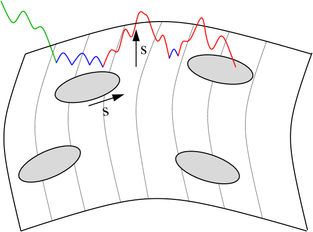
Figure 6: Cartoon of a cell surface with 4 receptors (gray ovals). A diffusing particle first hits the cell (green trajectory) and then makes 3 non-independent hits of the surface (blue), before an independent hit (red). The particle lands on a receptor after one more non-independent hit.

The first step in their argument relies on the feature that if a diffusing particle hits the surface of a sphere, it will hit again many times before diffusing away; this point was discussed above in Sec. 3. There are two types of subsequent hitting events: (i) the particle rises a distance less than $s$ above the surface before hitting it again, and (ii) the particle rises a distance greater than $s$ above the surface before hitting it again (Fig. 6). In the former case, if the particle initially misses a receptor, it will likely miss upon the second encounter. In the latter case, if the particle misses a receptor initially, we have no information about whether the second encounter will hit or miss a receptor. Thus the rise distance $s$ demarcates the regime of dependent subsequent hits and independent subsequent hits. It is the latter events that are relevant for estimating the reaction rate. We thus use the height $s$ as the criterion for determining the number of times that a particle independently hits the cell surface before diffusing away.

When a particle is a distance $s$ above the cell surface, the probability that it eventually hits the cell again is, using Eq. (6.2),

$$p_{s}=\frac{a}{a+s}\,.$$ (6.4a)

Thus the probability that the diffusing particle independently hits the cell $$n p_{s}^{n}(1-p_{s})$$ times before diffusing away is . Correspondingly, the average number of independent hits to the surface is

$$\langle n\rangle=\sum_{n>0}np_{s}^{n}\;(1-p_{s})=(1-p_{s})^{-1}=\frac{a+s}{s}\sim\frac{a}{s}\,.$$ (6.4b)

The probability for a diffusing particle to not land on a receptor in a single independent hitting event is

$$\beta=1-\frac{N\pi s^{2}}{4\pi a^{2}}\,,$$ (6.4c)

namely, the area fraction of the surface that is not covered by receptors. Thus the probability $p_{\rm escape}$ that a diffusing particle that reaches the cell but never lands on a receptor is the probability that the particle always misses a receptor in each of its independent hitting attempts. This is

$$p_{\rm escape}=\sum_{n>0}(\beta p_{s})^{n}(1-p_{s})=\frac{1-p_{s}}{1-\beta p_{s}}=\frac{4a}{4a+Ns}\,.$$ (6.4d)

The probability that a diffusing particle ultimately hits a receptor thus is

$$p_{\rm hit}=1-p_{\rm escape}=\frac{Ns}{4a+Ns}\,.$$ (6.4e)

The final result for the reaction rate of a cell of radius $a$ that is covered by $N$ receptors, each of radius $s$, is

$$k=4\pi Da\times\frac{Ns}{4a+Ns}\equiv 4\pi Da\times\text{efficiency}\,.$$ (6.5)

To understand the implication of this result, let’s use some numbers that typify a cell: $a=1$ micron, $s=10$ nanometers, and $N=10^{4}$. The area fraction covered by the receptors is roughly $10^{-3}$, but the absorption efficiency of the cell is roughly 2/3! Evidently, Mother Nature is very smart to not waste resources on endowing a cell with too many receptors.

7 Wedge Domains

We now turn to the first-passage properties of diffusion in a two-dimensional wedge domain with absorption when the particle hits the wedge boundary. One of our motivations for studying this system is that first passage in the wedge can be mapped onto a simple diffusive capture problem in one dimension that we’ll treat in the next section. We will obtain first-passage properties in the wedge geometry both by direct solution of the diffusion equation and also, for two dimensions, in a more aesthetically pleasing fashion by conformal transformation techniques, in conjunction with the electrostatic formulation. We also present a heuristic extension of the electrostatic approach that allows us to infer, with little additional computational effort, time-dependent first-passage properties in the wedge from corresponding time-integrated properties.

Solution to the Diffusion Equation

We first solve the diffusion equation in the wedge to determine the survival probability of a diffusing particle. While the exact Green’s function for this system is well known [12, 13], we adopt the strategy of choosing an initial condition that allows us to eliminate angular variables and deal with an effective radial problem. This simplification is appropriate if we are interested only in asymptotic first-passage properties.

The diffusion equation for the two-dimensional wedge geometry in plane polar co-ordinates is

$$\frac{\partial c}{\partial t}=D\left(\frac{\partial^{2}c}{\partial r^{2}}+\frac{1}{r}\frac{\partial c}{\partial r}+\frac{1}{r^{2}}\frac{\partial^{2}c}{\partial\theta^{2}}\right),$$ (7.1)

where $c=c(r,\theta,t)$ is the particle concentration at $(r,\theta)$ at time $t$, $D$ is the diffusion coefficient, and the boundary conditions are $c=0$ at $\theta=0,\Theta$, where $\Theta$ is the wedge opening angle. To reduce this two-dimensional problem to an effective one-dimensional radial problem, note that the exact Green’s function can be written as an eigenfunction expansion in which the angular dependence is a sum of sine waves of the form $\sin(n\pi\theta/\Theta)$, such that an integral number of half-wavelengths fit within $(0,\Theta)$ to satisfy the absorbing boundary conditions [13]. In this series, each sine wave is multiplied by a conjugate decaying function of time, in which the decay rate increases with $n$. In the long time limit, only the lowest term in this expansion dominates the survival probability. Consequently, we obtain the long-time behavior by choosing an initial condition whose angular dependence is a half sine-wave in the wedge. This ensures that the time-dependent problem will contain only this single term in the Fourier series.

We therefore define $c(r,\theta,t=0)=\pi\delta(r-r_{0})/(2\Theta r_{0})\times\sin(\pi\theta/\Theta)$. With this initial distribution function and after the Laplace transform is applied, the diffusion equation (7.1) becomes

$$sc(r,\theta,s)-\frac{\pi}{2\Theta r_{0}}\delta(r-r_{0})\sin(\pi\theta/\Theta)=D\left(\frac{\partial c^{2}}{\partial r^{2}}+\frac{1}{r}\frac{\partial c}{\partial r}+\frac{1}{r^{2}}\frac{\partial^{2}c}{\partial\theta^{2}}\right)\,,$$

where $c=c(r,\theta,s)$. Substituting in the ansatz $c(r,\theta,s)=R(r,s)\sin(\pi\theta/\Theta)$, the angular dependence may now be separated and reduces the system to an effective one-dimensional radial problem. By introducing the dimensionless co-ordinate $x=r\sqrt{s/D}$, we find the modified Bessel equation for the remaining radial co-ordinate,

$$R^{\prime\prime}(x,s)+\frac{1}{x}R^{\prime}(x,s)-\left(1+\frac{\nu^{2}}{x^{2}}\right)R(x,s)=-\frac{\nu}{2Dx_{0}}\delta(x-x_{0}),$$ (7.2)

where $\nu=\pi/\Theta$ and the prime now denotes differentiation with respect to $x$.

The general solution for $x\neq x_{0}$ is a superposition of modified Bessel functions of order $\nu$. Since the domain is unbounded, the interior Green’s function ($x<x_{0}$) involves only $I_{\nu}$, since $K_{\nu}$ diverges as $x\to 0$, while the exterior Green’s function ($x>x_{0}$) involves only $K_{\nu}$, since $I_{\nu}$ diverges as $x\to\infty$. By imposing continuity at $x=x_{0}$, we find that the Green’s function has the symmetric form $R(x,s)=AI_{\nu}(x_{<})K_{\nu}(x_{>})$, with the constant $A$ determined by the joining condition that arises from integrating Eq. (7.2) over an infinitesimal radial range that includes $r_{0}$. This gives

$$R_{>}^{\prime}\mid_{x=x_{0}}-R_{<}^{\prime}\mid_{x=x_{0}}=-\frac{\nu}{2Dx_{0}}\,,$$

from which $A=\nu/2D$. Therefore the radial Green’s function in the wedge is

$$R(x,s)=\frac{\nu}{2D}\,I_{\nu}(x_{<})\,K_{\nu}(x_{>}),$$ (7.3)

and its Laplace inverse has the relatively simple closed form [12, 13]

$$R(r,t)=\frac{\nu}{4Dt}\,\,e^{-(r^{2}+r_{0}^{2})/4Dt}\,\,I_{\nu}\left(\frac{rr_{0}}{2Dt}\right).$$ (7.4)

With this radial Green’s function, the asymptotic survival probability is

$$S(t)\sim\int_{0}^{\Theta}\sin(\nu\theta)\,d\theta\,\int_{0}^{\infty}r\,R(r,t)\,dr.$$ (7.5)

We can estimate this integral by noting that the radial distance over which the concentration is appreciable extends to the order of $\sqrt{Dt}$. This provides a cutoff $r\approx\sqrt{Dt}$ in the radial integral in Eq. (7.5), within which the Gaussian factors in $R(r,t)$ can be replaced by one. Using the small-argument expansion of the Bessel function, we then obtain

$$S(t)=\int_{0}^{\Theta}\!\!\!\sin(\nu\theta)\,d\theta\,\int_{0}^{\infty}\!\!\!r\,R(r,t)\,dr\propto\int_{0}^{\sqrt{Dt}}\!\frac{1}{Dt}\left(\frac{rr_{0}}{Dt}\right)^{\nu}\,r\,dr\sim\left(\frac{r_{0}}{\sqrt{Dt}}\right)^{\pi/\Theta}.$$ (7.6)

The basic result is that the survival probability of a diffusing particle in a wedge of opening angle $\Theta$ decays with time as

$$S(t)\sim t^{-\pi/2\Theta}\equiv t^{-\alpha}.$$ (7.7)

The striking feature of this formula is that the exponent $\alpha$ depends on the wedge opening angle in a non-trivial way, with $\alpha\to\infty$ as $\Theta\to 0$ and $\alpha\to 1/4$ for $\Theta\to 2\pi$.

Conformal Transformations and Electrostatic Methods

Let’s now solve the same wedge problem by exploiting conformal transformations, together with the connection between first passage and electrostatics. To set the stage for the wedge geometry, consider the first-passage probability for a diffusing particle in two dimensions to an absorbing infinite line. This problem may also be solved elegantly by the electrostatic formulation. In this approach, the time-integrated concentration $\mathcal{C}(x,y)=\int_{0}^{\infty}c(x,y,t)\,dt$ obeys the Laplace equation

$$\nabla^{2}\mathcal{C}(z)=-\frac{1}{2\pi D}\;\delta(z-z_{0})\,,$$

where $z=(x,y)$ is the complex co-ordinate and the factor $1/(2\pi D)$ ensures the correct normalization. Using the image method for two-dimensional electrostatics, we find that the complex potential is

$$\mathcal{C}(z)=\frac{1}{2\pi D}\ln\frac{z-z_{0}}{z-z_{0}^{*}}=\frac{1}{2\pi D}\ln\frac{x-x_{0}+i(y-y_{0})}{x-x_{0}+i(y+y_{0})},$$ (7.8)

where the asterisk denotes complex conjugation. Finally, the time-integrated flux that is absorbed at $x$ coincides with the electric field at this point. This is

$${\mathcal{E}}(x|x_{0},y_{0}) =-D\,\frac{\partial\mathcal{C}(x,y)}{\partial y}\bigg{|}_{y=0}$$

$$=\frac{1}{2\pi}\left(\frac{1}{y_{0}+i(x-x_{0})}+\frac{1}{y_{0}-i(x-x_{0})}\right)$$

$$=\frac{1}{\pi}\frac{y_{0}}{(x-x_{0})^{2}+y_{0}^{2}}\,.$$ (7.9)

We now use a conformal transformation to extend the result for the hitting probability to the infinite line to the hitting probability in the wedge. Consider the transformation $w=f(z)=z^{\pi/\Theta}$ that maps the interior of the wedge of opening angle $\Theta$ to the upper half plane. In complex co-ordinates, the electrostatic potential in the wedge is

$$\mathcal{C}(z)=\frac{1}{2\pi D}\ln\frac{z^{\pi/\Theta}-z_{0}^{\pi/\Theta}}{z^{\pi/\Theta}-(z_{0}^{*})^{\pi/\Theta}}.$$ (7.10)

From this expression and using the analogy between electrostatics and first passage, we can extract time-integrated first-passage properties in the wedge. For example, the probability of being absorbed at a distance $x$ from the wedge apex, when a particle begins at a unit distance from the apex along the wedge bisector, is just the electric field at this point

$${\mathcal{E}}(x|x_{0},y_{0})=\frac{1}{\Theta}\frac{x^{\pi/\Theta-1}}{1+x^{2\pi/\Theta}}\to x^{-(1+\pi/\Theta)}\qquad\text{for~{}}x\to\infty\,.$$ (7.11)

Although the electrostatic formulation ostensibly gives only time-integrated first-passage properties, we can adapt it to also give time-dependent features. This adaptation is based on the following re-interpretation of the equivalence between electrostatics and diffusion: an electrostatic system with a point charge and specified boundary conditions is identical to a diffusive system in the same geometry and boundary conditions, in which a continuous source of particles is fed in at the location of the charge starting at time $t=-\infty$. Suppose now that the particle source is “turned on” at $t=0$. Then, in a near zone that extends out to a distance of the order of $\sqrt{Dt}$ from the source, the concentration has sufficient time to reach its steady-state value. Within this zone, the diffusive solution converges to the Laplacian solution. Outside this zone, however, the concentration is close to zero. This almost-Laplacian solution provides the time integral of the survival probability up to time $t$. We can then deduce the survival probability by differentiating the concentration that is due to this finite-duration source.

Thus suppose that a constant source of diffusing particles at $z_{0}$ inside the absorbing wedge is turned on at $t=0$. Within the region where the concentration has had time to reach the steady state, $|z_{0}|<|z|<\sqrt{Dt}$, the density profile is approximately equal to the Laplacian solution, $\mathcal{C}(z)\sim|z|^{-\pi/\Theta}$. We can neglect the angular dependence of $\mathcal{C}(z)$ in this zone, as this dependence is immaterial for the survival probability. Conversely, for $|z|>\sqrt{Dt}$, the particle concentration is vanishingly small because a particle is unlikely to diffuse such a large distance. From the analogy between electrostatics and first passage, the near-zone density profile is just the same as the time integral of the diffusive concentration. Thus, by using the equivalence between the spatial integral of this near-zone concentration in the wedge and the time integral of the survival probability, we have

$$\int_{0}^{t}S(t^{\prime})\,dt^{\prime}\approx\int_{0}^{\sqrt{Dt}}r^{-\pi/\Theta}\,r\,dr\sim t^{1-\pi/2\Theta}.$$ (7.12)

Since the total density injected into the system equals $t$, the survival probability in the wedge is roughly $\int_{0}^{t}S(t^{\prime})\,dt^{\prime}/t\sim t^{1-\pi/2\Theta}/t$, which gives $S(t)\sim t^{-\pi/2\Theta}$.

8 Stochastic Hunting in One Dimension

What is the time dependence of the survival probability of a diffusing lamb that is hunted by $N$ diffusing lions? We define this survival probability as $S_{N}(t)$. This toy problem is most interesting in a one-dimensional geometry where all the lions are located to one side of the lamb. It is known [14] that this survival probability asymptotically decays algebraically with time,

$$S_{N}(t)\sim t^{-\beta_{N}}\,,$$ (8.1)

and the goal is to compute the decay exponent $\beta_{N}$. As we shall discuss, the decay exponent is known for $N=1$ and $N=2$ only: $\beta_{1}=\frac{1}{2}$, and $\beta_{2}=\frac{3}{4}$. For $N\geq 3$, $\beta_{N}$ grows slowly with $N$, and numerical simulations give $\beta_{3}\approx 0.91$, $\beta_{4}\approx 1.03$, and $\beta_{10}\approx 1.4$. The focus of this section is to derive $\beta_{2}=\frac{3}{4}$ by a simple geometric approach and to develop some analytical understanding of the dependence of $\beta_{N}$ on $N$ for $N\to\infty$.

Let us begin by treating a lamb that starts at $x_{0}>0$ and a single lion that starts at $x=0$. For simplicity, the diffusivities of the lamb and the lion are assumed to both equal $D$. The separation between the lamb and the lion thus diffuses with diffusion coefficient $2D$. When this separation reaches zero, the lamb has been eaten. This problem is just the classic first-passage problem on the positive infinite line, except that the diffusion coefficient is $2D$. The probability that the lamb survives until time $t$ is the same as the first-passage time being greater than $t$. This probability therefore is

$$S_{1}(t) =\int_{t}^{\infty}\!\frac{x_{0}}{\sqrt{8\pi Dt^{\prime 3}}}\;e^{-x_{0}^{2}/8Dt^{\prime}}\,dt^{\prime}=\text{erf}\biggl{(}\frac{x_{0}}{\sqrt{8Dt}}\biggr{)}\sim\frac{x_{0}}{\sqrt{8\pi Dt}}\,.$$ (8.2)

Thus the survival probability of the lamb asymptotically decays as $t^{-1/2}$. While the lamb is sure to die, its average lifetime is infinite. Thus a single diffusing lion is not a particularly good hunter and it might starve before eating the lamb.

What happens when there are $N=2$ lions? We again assume that the lions start from the origin while the lamb starts at $x_{0}>0$, and that the diffusivities of all particles are the same. Let us label the positions of the lions as $x_{1}$ and $x_{2}$, and the position of the lamb as $x_{3}$ The lamb survives up to time $t$ if the conditions $x_{3}>x_{2}$ and $x_{3}>x_{1}$ always hold. We can give an insightful geometric interpretation of this problem by viewing the motion of the three particles on the line as equivalent to the motion of a single effective particle in three dimensions with coordinates $(x_{1},x_{2},x_{3})$. The constraints $x_{3}>x_{2}$ and $x_{3}>x_{1}$ mean that the effective particle in three-space remains to the left of the plane $x_{2}=x_{3}$ and behind the plane $x_{1}=x_{3}$ (Fig. 7(a)). This allowed region is a wedge of opening angle $\Theta$ that is defined by the intersection of these two planes. If the particle hits one of the planes, then one of the lions has eaten the lamb.

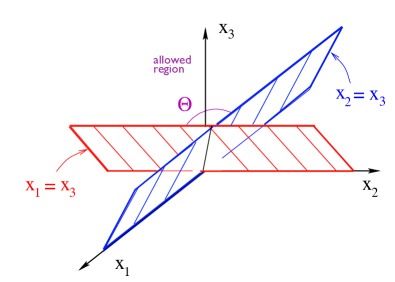
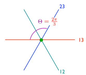
Figure 7: (a) The allowed region for the effective particle that corresponds to the motion of the lamb and two lions. (b) A view of the constraint planes perpendicular to the (1,1,1) axis. The constraint plane $x_{1}=x_{2}$ is also shown

This mapping therefore provides the lamb survival probability, since the survival probability of a diffusing particle within this absorbing wedge asymptotically decays as $S_{\rm wedge}(t)\sim t^{-\pi/2\Theta}$. What is the opening angle of this wedge? We can determine this angle in a simple way by also including the plane $x_{1}=x_{2}$ and then viewing the system along the $(1,1,1)$ axis (Fig. 7(b)). It is then clear that the wedge angle is $2\pi/3$. Substituting this result in Eq. (7.7), we find that $\beta_{2}=\frac{3}{4}$. Notice that $S_{2}(t)>S_{1}(t)^{2}$. This inequality reflects the fact that the incremental threat to the lamb from the second lion is less than the first.

In general, we can map the motion of the lamb and $N$ lions in one dimension to a single effective particle in $N+1$ dimensions, with absorption when the effective particle hits any of the $N$ constraint planes. However, the calculation of the survival probability of the effective particle within the domain where the effective particle is confined—known as a Weyl chamber—appears to be intractable.

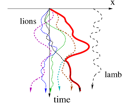
Figure 8: Space-time trajectories of 6 lions and 1 lamb. Although the motion of each lion is isotropic, the trajectory of the lion (whose identity may change) that happens to be closest to the lamb (solid red curve) tends to move towards the lamb.

While the problem for $N=3,4,\ldots$ lions is difficult, the problem becomes much simpler for large $N$. To determine the lamb survival probability for large $N$, we only need to focus on the lion closest to the lamb, because this last lion ultimately kills the lamb. As shown in Fig. 8, the individual identity of this last lion can change with time due to the crossing of different lion trajectories. For large $N$, there is a systematic bias of the motion of the last lion, $x_{\rm last}(t)$. This bias becomes stronger for increasing $N$, so that $x_{\rm last}(t)$ becomes smoother as $N$ increases (Fig. 9). This gradual approach of the last lion to the lamb is the mechanism which leads to the survival probability of the lamb decaying as $t^{-\beta_{N}}$, with $\beta_{N}$ a slowly increasing function of $N$.

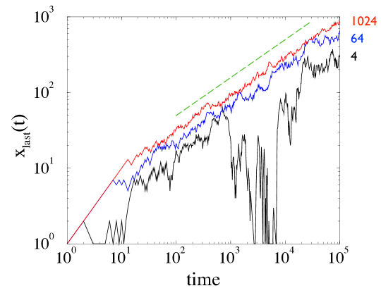
Figure 9: Position of the last lion versus time for 4, 64, and 1024 lions.

To estimate the location of this last lion when $N\gg 1$ lions are initially at the origin, we use the extreme statistics condition [15]

$$\int_{x_{\rm last}}^{\infty}\frac{N}{\sqrt{4\pi Dt}}\,e^{-x^{2}/4Dt}\,\,dx=1.$$ (8.3)

Equation (8.3) states that one lion out of an initial group of $N$ is in the range $[x_{\rm last},\infty]$. Although the integral in Eq. (8.3) can be expressed in terms of the complementary error function, it is instructive to evaluate it approximately in a self consistent way by writing $x=x_{\rm last}+\epsilon$ and re-expressing the integrand in terms of $\epsilon$. We thus find

$$\int_{0}^{\infty}\frac{N}{\sqrt{4\pi Dt}}\,e^{-x_{\rm last}^{2}/4Dt}\,e^{-x_{\rm last}\epsilon/2Dt}\,e^{-\epsilon^{2}/4Dt}\,\,d\epsilon=1.$$

Now the second term in the integrand,

$$e^{-x_{\rm last}\epsilon/2Dt}\,,$$

is non-negligible for $\epsilon<2Dt/x_{\rm last}$. Over this range of $\epsilon$, the third exponential factor is of the order of

$$e^{-Dt/x_{\rm last}^{2}}\,.$$

If we use the result for $x_{\rm last}$ in Eq. (8.5), the above exponential factor becomes

$$e^{-1/(4\ln N)}\,,$$

which is very close to 1 for large N. If we thus ignore this term, the integral above reduces to simple exponential decay, with the result

$$\frac{N}{\sqrt{4\pi Dt}}\,e^{-x_{\rm last}^{2}/4Dt}\,\frac{2Dt}{x_{\rm last}}=1.$$ (8.4)

We now define $y=x_{\rm last}/\sqrt{4Dt}$ and $M=N/\sqrt{4\pi}$, so that the above condition can be simplified to $y\exp(e^{y^{2}})=M$, whose asymptotic solution is

$$y=\sqrt{\ln M\,}\Bigl{(}1-\frac{1}{4}\frac{\ln(\ln M)}{\ln M}+\ldots\Bigr{)}.$$

To lowest order, this gives

$$x_{\rm last}(t)\sim\sqrt{4D\ln N\,t}\equiv\sqrt{A_{N}t},$$ (8.5)

for $N$ finite. For $N=\infty$, $x_{\rm last}(t)$ would always equal $t$ if an infinite number of discrete random walking lions were initially at the origin. A more suitable initial condition therefore is a concentration $c_{0}$ of lions that are uniformly distributed from $-\infty$ to 0. In this case, only $N\propto\sqrt{c^{2}_{0}Dt}$ of the lions are “dangerous,” that is, within a diffusion distance from the edge of the pack and thus potential candidates for eating the lamb. Consequently, for $N\to\infty$, the leading behavior of $x_{\rm last}(t)$ becomes

$$x_{\rm last}(t)\sim\sqrt{2D\ln(c^{2}_{0}Dt)\,t}\,.$$ (8.6)

An important feature of the time dependence of $x_{\rm last}$ is that fluctuations in this quantity decrease for large $N$ (Fig. 9). Therefore the lamb and $N$ diffusing lions can be recast as a two-body system of a lamb and an absorbing boundary which deterministically advances toward the lamb according to $x_{\rm last}(t)=\sqrt{A_{N}t}$. This determinism is what makes the problem for large $N$ tractable.

To solve this effective two-body problem, it is convenient to change coordinates from $(x,t)$ to $(^{\prime}=x-x_{\rm last}(t),t)$ to fix the absorbing boundary at the origin. By this construction, the diffusion equation for the lamb probability distribution is transformed to the convection-diffusion equation

$$\frac{\partial p(x^{\prime},t)}{\partial t}-\frac{x_{\rm last}}{2t}\frac{\partial p(x^{\prime},t)}{\partial x^{\prime}}=D\frac{\partial^{2}p(x^{\prime},t)}{\partial x^{\prime 2}}\,,\quad(0\leq x^{\prime}<\infty)$$ (8.7)

with the absorbing boundary condition $p(x^{\prime}=0,t)=0$. In this reference frame that is fixed on the average position of the last lion, the second term in Eq. (8.7) accounts for the bias of the lamb towards the absorber with an effective speed $-x_{\rm last}/2t$. Because $x_{\rm last}\sim\sqrt{A_{N}t}$ and $x^{\prime}\sim\sqrt{Dt}$ have the same time dependence, the lamb survival probability acquires a nontrivial dependence on the dimensionless parameter $A_{N}/D$. This behavior arises whenever there is a coincidence of fundamental length scales in the system (see, e.g., [16] for other such examples).

Equation (8.7) can be transformed into the parabolic cylinder equation by first introducing the dimensionless length $\xi=x^{\prime}/x_{\rm last}$ and making the following scaling ansatz for the lamb probability density,

$$p(x^{\prime},t)\sim t^{-\beta_{N}-1/2}\mathcal{C}(\xi).$$ (8.8)

The power law prefactor in Eq. (8.8) ensures that the integral of $p(x^{\prime},t)$ over all space, namely the survival probability, decays as $t^{-\beta_{N}}$, and $\mathcal{C}(\xi)$ expresses the spatial dependence of the lamb probability distribution in scaled length units. This ansatz codifies the fact that the probability density is not a function of $x^{\prime}$ and $t$ separately, but is a function only of the dimensionless ratio $x^{\prime}/x_{\rm last}(t)$.

Substituting Eq. (8.8) into Eq. (8.7), we obtain

$$\frac{D}{A_{N}}\frac{d^{2}{\mathcal{C}}}{d\xi^{2}}+\frac{1}{2}(\xi+1)\frac{d\mathcal{C}}{d\xi}+\bigl{(}\beta_{N}+\frac{1}{2}\bigr{)}\mathcal{C}=0.$$ (8.9)

By introducing $\eta=(\xi+1)\sqrt{A_{N}/2D}$ and $\mathcal{C}(\xi)=e^{-\eta^{2}/4}\,{\mathcal{D}}(\eta)$ in Eq. (8.9), we are led to the parabolic cylinder equation of order $2\beta_{N}$ [17]

$$\frac{d^{2}{\mathcal{D}}_{2\beta_{N}}}{d\eta^{2}}+\biggl{[}2\beta_{N}+\frac{1}{2}-\frac{\eta^{2}}{4}\biggr{]}{\mathcal{D}}_{2\beta_{N}}=0,$$ (8.10)

subject to the boundary condition, ${\mathcal{D}}_{2\beta_{N}}(\eta)=0$ for both $\eta=\sqrt{A_{N}/2D}$ and $\eta=\infty$. Equation (8.10) has the form of a Schrödinger equation for a quantum particle of energy $2\beta_{N}+\frac{1}{2}$ in a harmonic oscillator potential $\eta^{2}/4$ for $\eta>\sqrt{A_{N}/2D}$, but with an infinite barrier at $\eta=\sqrt{A_{N}/D}$ [18]. For the long-time behavior, we need to find the ground state energy in this potential. For $N\gg 1$, we may approximate this energy as the potential at the classical turning point, that is, $2\beta_{N}+\frac{1}{2}\simeq\eta^{2}/4$. We therefore obtain $\beta_{N}\sim A_{N}/16D$. Using the value of $A_{N}$ given in Eqs. (8.5) and (8.6) the decay exponent is

$$\beta_{N}\sim\begin{cases}\tfrac{1}{4}\ln N&N~{}\text{finite}\\[5.69054pt] \tfrac{1}{8}\ln t&N=\infty\,.\end{cases}$$ (8.11)

The latter dependence of $\beta_{N}$ implies that for $N\to\infty$, the survival probability has the log-normal form

$$S_{\infty}(t)\sim\exp\left(-\tfrac{1}{8}\,\ln^{2}t\right).$$ (8.12)

The important feature of the exponent $\beta_{N}$ is its very slow increase with $N$. That is, each successive lion that is added to the hunt has a decreasing influence on the survival of the lamb. Indeed, only a small subset of the lions for large $N$ actually have a chance to catch the lamb.

9 The Expanding Interval

We have seen that the survival probability $S(t)$ of a diffusing particle in a fixed-length absorbing interval of length $L$ asymptotically decays as $e^{-\pi^{2}Dt/L^{2}}$. What happens if the interval length grows with time, $L(t)\sim t^{\alpha}$? This simple question illustrates the relative effects of diffusion and the motion of the boundary on first-passage properties. This interplay is a classic problem in the first-passage literature, especially when the boundary motion matches that of diffusion. Solutions to this problem have been obtained by a variety of methods (see, e.g., [19, 20, 21, 22]). Here we give a physics-based approach that is based on [23].

It is easy to infer the survival probability for a slowly expanding interval. Here, slowly expanding means that the interval length grows slower than diffusion. Consequently, the probability distribution of the particle spreads faster than the interval grows and so that the survival probability should decay rapidly with time. Using an adiabatic approximation that one typically encounters in basic quantum mechanics, we will show that $S(t)\sim\exp\big{[}-At^{(1-2\alpha)}\big{]}$, where $A$ is a constant. Conversely, for the rapidly expanding interval, $\alpha>1/2$, the particle is unlikely reach the either end of the interval and the probability distribution is close to that for free diffusion. This is the basis of the free approximation that leads to a non-zero limiting value for $S(t)$ as $t\to\infty$.

In the marginal case where the interval expands at the same rate as diffusion, $L(t)=\sqrt{At}$, a new dimensionless parameter arises—the ratio of the diffusion length to the interval length. As we shall show, this leads to $S(t)$ decaying as a non-universal power-law in time, $S(t)\sim t^{-\beta}$, with $\beta=\b{(}A,D)$ diverging for $A/D\ll 1$ and approaching zero for $A/D\gg 1$.

Slowly Expanding Interval

For $L(t)\ll\sqrt{Dt}$, we invoke the adiabatic approximation [18], in which the spatial dependence of the concentration for an interval of length $L(t)$ is assumed to be identical to that of the static diffusion equation at the instantaneous value of $L$. This assumption is based on the expectation that the concentration in a slowly expanding interval is always close to that of a fixed-size interval. Thus we write

$$c(x,t)\simeq f(t)\,\cos\left(\frac{\pi x}{2L(t)}\right)\equiv c_{\rm ad}(x,t),$$ (9.1)

with $f(t)$ to be determined. The corresponding survival probability is

$$S(t)\approx\int_{-L(t)}^{L(t)}~{}c_{\rm ad}(x,t)\,dx=\frac{4}{\pi}~{}f(t)L(t).$$ (9.2)

For convenience, we now define the interval boundaries as $[-L(t),L(t)]$. To obtain $f(t)$, we substitute approximation (9.1) into the diffusion equation, as in separation of variables, to give

$$\frac{df}{dt}=-\left(\frac{D\pi^{2}}{4L^{2}}\right)f-\left(\frac{\pi x}{2L^{2}}\right)\,\frac{dL}{dt}\,\tan\left(\frac{\pi x}{2L}\right)\,f.$$ (9.3)

Notice that variable separation does not strictly hold, since the equation for $f(t)$ also involves $x$. However, when $L(t)$ increases as $(At)^{\alpha}$ with $\alpha<1/2$, the second term on the right-hand side is negligible. Thus we drop this second term and solve the simplified form of (9.3). We thereby find that the controlling factor of $f(t)$ is given by

$$f(t)\sim\exp\left[-\frac{D\pi^{2}}{4}\int_{0}^{t}\,\frac{dt^{\prime}}{L^{2}(t^{\prime})}\right]=\exp\left[-\frac{D\pi^{2}}{4(1-2\alpha)A^{2\alpha}}\,t^{1-2\alpha}\right].$$ (9.4)

Notice that $f(t)$ reduces to a pure exponential decay for a fixed-length interval, while for $\alpha\to 1/2$, Eq. (9.4) suggests a more slowly decaying functional form for $S(t)$.

Rapidly Expanding Interval

For a rapidly expanding interval, the escape rate from the system is small and the absorbing boundaries should eventually become irrelevant. We therefore expect that the concentration profile should approach the Gaussian distribution of free diffusion at long times [23]. We may then account for the slow decay of the survival probability by augmenting the Gaussian with an overall decaying amplitude. This free approximation is a nice example in which the existence of widely separated time scales, $\sqrt{Dt}$ and $L(t)$, suggests the nature of the approximation itself.

According to the free approximation, we write

$$c(x,t)\approx\frac{S(t)}{\sqrt{4\pi Dt}}\,e^{-x^{2}/4Dt}\equiv c_{\rm free}(x,t)\,.$$

Although this concentration does not satisfy the absorbing boundary condition, the inconsistency is negligible at large times, since the density is exponentially small at the interval boundaries. We may now find the time dependence of the survival probability by equating the probability flux to the interval boundaries, $2D|\frac{\partial c}{\partial x}|$, to the loss of probability within the interval. For $L(t)=(At)^{\alpha}$, this flux is

$$\frac{S(t)A^{\alpha}}{\sqrt{4\pi D}}\;t^{\alpha-3/2}\,\exp\left(-\frac{A^{2\alpha}}{4D}t^{2\alpha-1}\right),$$ (9.5)

which rapidly goes to zero for $\alpha>1/2$. Since this flux equals $-\frac{dS}{dt}$, it follows that the survival probability approaches a non-zero limiting value for $\alpha>1/2$, and that this limiting value goes to zero as $\alpha\to 1/2$. Explicitly,

$$\frac{dS(t)}{dt}=-\frac{1}{S(t)}\;B\,t^{\alpha-3/2}\;\exp\left(-C\,t^{2\alpha-1}\right)\,,$$ (9.6)

where $B\equiv A^{\alpha}/\sqrt{4\pi D}$ and $C\equiv A^{2\alpha}/(4D)$. We now introduce $y=Ct^{2\alpha-1}$ and change the integration variable from $t$ to $y$. After some straightforward steps we have

$$\ln S(t\!=\!\infty) =-\frac{B}{2\alpha-1}\int_{0}^{\infty}\left(\frac{y}{C}\right)^{1/2}e^{-y}\;\frac{dy}{y}$$

$$=-\frac{B}{C^{1/2}}\frac{1}{2\alpha-1}\,\Gamma\left(\tfrac{1}{2}\right)\,,$$ (9.7)

where $\Gamma(\cdot)$ is the Euler gamma function. Thus a diffusing particle has a non-zero probability to survive forever when the interval grows fast enough. This ultimate survival probability rapidly goes to zero as $\alpha\to 1/2$ from above.

Marginally Expanding Interval

For the marginal case of $\alpha=1/2$, the adiabatic and the free approximations are ostensibly no longer appropriate, since $L(t)=\sqrt{At}$ and $\sqrt{Dt}$ have a fixed ratio. However, for $A/D\ll 1$ and $A/D\gg 1$, we might hope that these methods could still be useful. Thus we continue to apply these heuristic approximations in their respective domains of validity, $A/D\ll 1$ and $A/D\gg 1$, and check their accuracies a posteriori. We will see that the survival probability exponents predicted by these two approximations are each quite close to the exact result except for $A/D\approx 1$.

When the adiabatic approximation is applied, the second term in Eq. (9.3) is, in principle, non-negligible for $\alpha=1/2$. However, for $A\ll D$, the interval still expands more slowly (in amplitude) than free diffusion and the error made by neglecting the second term in Eq. (9.3) may still be small. The solution to this crudely truncated equation immediately gives $f(t)$, which, when substituted into approximately (9.2) leads to $S_{\rm ad}(t)\approx t^{-\beta_{\rm ad}}$, with

$$\beta_{\rm ad}\approx\frac{D\pi^{2}}{4A}-\frac{1}{2}.$$ (9.8)

The trailing factor of $-1/2$ should not be taken very seriously, because the neglected term in Eq. (9.3) leads to additional corrections to $\beta_{\rm ad}$ that are also of the order of 1.

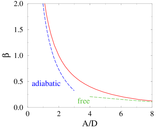
Figure 10: The survival probability exponent $\beta$ for the marginal case $L(t)=(At)^{1/2}$. Shown is the numerically exact value of $\beta$ (red, solid) from solution of Eq. (9.13), together with the predictions from the adiabatic and the free approximations, Eqs.(9.8) and (9.10) respectively (dashed curves).

Similarly for $A\gg D$, the free approximation gives

$$\frac{dS}{dt}\approx-2D\bigg{|}\frac{\partial c(x,t)}{\partial x}\bigg{|}_{x=\sqrt{At}}\;=\,-\frac{S(t)}{t}\sqrt{\frac{A}{4\pi D}}\,e^{-A/4D}.$$ (9.9)

This again leads to the non-universal power law for the survival probability, $S_{\rm free}\sim t^{-\beta_{\rm free}}$, with

$$\beta_{\rm free}=\sqrt{\frac{A}{4\pi D}}\,e^{-A/4D}.$$ (9.10)

As shown in Fig. 10, these approximations are surprisingly accurate over much of the range of $A/D$.

To complete our discussion, we outline a first-principles analysis for the survival probability of a diffusing particle in a marginally expanding interval [23]. When $L(t)=\sqrt{At}$, a natural scaling hypothesis is to write the density in terms of the two dimensionless variables

$$\xi\equiv\frac{x}{L(t)}\qquad{\rm and}\qquad\rho=\sqrt{\frac{A}{D}}\,.$$

We now seek solutions for the concentration in the form,

$$c(x,t)=t^{-\beta-1/2}\;\mathcal{C}_{\rho}(\xi),$$ (9.11)

where $\mathcal{C}_{\rho}(\xi)$ is a two-variable scaling function that encodes the spatial dependence. The power law prefactor ensures that the survival probability, namely, the spatial integral of $c(x,t)$, decays as $t^{-\beta}$, as defined at the outset of this section.

After substituting Eq. (9.11) into the diffusion equation, the scaling function satisfies the ordinary differential equation

$$\frac{1}{\rho^{2}}\frac{d^{2}\mathcal{C}}{d\xi^{2}}+\frac{\xi}{2}\frac{d\mathcal{C}}{d\xi}+\left(\beta+\frac{1}{2}\right)\mathcal{C}=0\,.$$

Then by introducing $\eta=\xi\,\sqrt{\rho/2}$ and $\mathcal{C}(\xi)=e^{-\eta^{2}/4}\,{\mathcal{D}}(\eta)$, we transform this into the parabolic cylinder equation [25]

$$\frac{d{\mathcal{D}}}{d\eta^{2}}+\left[2\beta+\frac{1}{2}-\frac{\eta^{2}}{4}\right]{\mathcal{D}}=0.$$ (9.12)

When the range of $\eta$ is unbounded, this equation has solutions for quantized values of the energy eigenvalue $E=2\beta+\frac{1}{2}=\frac{1}{2}$, $\frac{3}{2}$, $\frac{5}{2},\ldots$ [18].

For our interval problem, the range of $\eta$ is restricted to $|\eta|\leq\sqrt{A/2D}$. In the equivalent quantum mechanical system, this corresponds to a particle in a harmonic-oscillator potential for $|\eta|<\sqrt{A/2D}$ and an infinite potential for $|\eta|>\sqrt{A/2D}$. For this geometry, a spatially symmetric solution to Eq. (9.12), appropriate for the long-time limit for an arbitrary starting point, is

$${\mathcal{D}}(\eta)\equiv\tfrac{1}{2}\big{[}{\mathcal{D}}_{2\beta}(\eta)+{\mathcal{D}}_{2\beta}(-\eta)\big{]}\,,$$

where ${\mathcal{D}}_{\nu}(\eta)$ is the parabolic cylinder function of order $\nu$. Finally, the relation between the decay exponent $\beta$ and $\sqrt{A/D}$ is determined implicitly by the absorbing boundary condition, namely,

$${\mathcal{D}}_{2\beta}(\sqrt{A/2D})+{\mathcal{D}}_{2\beta}(-\sqrt{A/2D})=0.$$ (9.13)

This condition for $\beta=\beta(A/D)$ simplifies in the limiting cases $A/D\ll 1$ and $A/D\gg 1$. In the former, the exponent $\beta$ is large and the second two terms in the brackets in Eq. (9.12) can be neglected. Equivalently, the physical range of $\eta$ is small, so that the potential plays a negligible role. The solution to this limiting free-particle equation is just the cosine function, and the boundary condition immediately gives the limiting expression of Eq. (9.8), but without the subdominant term of $-1/2$. In the latter case of $A\gg D$, $\beta\to 0$ and Eq. (9.12) approaches the Schrödinger equation for the ground state of the harmonic oscillator. In this case, a detailed analysis of the differential equation reproduces the limiting exponent of Eq. (9.10) (see [23] for details). These provide rigorous justification for the limiting values of the decay exponent $\beta$ which we obtained by heuristic means.

The Khintchine Iterated Logarithm Law

In the marginal situation of $L(t)=(At)^{1/2}$, we have seen that the survival probability $S(t)$ decays as a power law $t^{-\beta(A,D)}$, with $\beta\to 0$ as $A/D\to\infty$. This decay becomes progressively slower as $A$ increases. On the other hand, when $L(t)\propto t^{\alpha}$, with $\alpha$ strictly greater than 1/2, the survival probability at infinite time is greater than zero. This leads to the following natural question: what is the nature of the transition between certain death, defined as $S(t\to\infty)=0$, and a non-zero survival survival probability, $S(t\to\infty)>0$?

The answer to this question is surprisingly rich. There is an infinite sequence of transitions, where $L(t)$ acquires additional iterated logarithmic time dependences, which define regimes where $S(t)$ assumes progressively slower functional forms. The first term in this series is known as the Khintchine iterated logarithm law ([24, 3]). While the Khintchine law has been obtained by rigorous methods, we can also obtain this intriguing result, as well as the infinite sequence of transitions, with relatively little computation by the free approximation.

Because we anticipate that the transition between life and death occurs when $L(t)$ grows slightly faster than $(At)^{1/2}$, we make the hypothesis that $A\propto u(t)$, with $u(t)$ growing slower than a power law in $t$. Now that $L(t)$ increases more rapidly than the diffusion length $(Dt)^{1/2}$, the free approximation should be asymptotically exact, since it already works extremely well when $L(t)=(At)^{1/2}$ with $A$ large. Within this approximation, we rewrite Eq. (9.9) as

$$\ln S(t)\sim-\int^{t}\frac{dt^{\prime}}{t^{\prime}}\sqrt{\frac{A}{4\pi D}}\,e^{-A/4D}.$$ (9.14)

Here we neglect the lower limit, since the free approximation is valid only as $t\to\infty$, where the short-time behavior is irrelevant. In this form, it is clear that for $L=(At)^{1/2}$, $\ln S$ decreases by an infinite amount for $t\to\infty$ because of the divergence of the integral. Thus $S(t\to\infty)\to 0$. To make the integral converge, the other factors in the integral must somehow cancel the logarithmic divergence that arises from the factor $dt/t$. Accordingly, let us substitute $L(t)=\sqrt{4Dt\,u(t)}$ into the approximation (9.14). This gives

$$\ln S(t)\sim-\frac{1}{\sqrt{\pi}}\int^{t}\frac{dt^{\prime}}{t^{\prime}}\sqrt{u(t^{\prime})}\,e^{-u(t^{\prime})}.$$

To simplify this integral, it is helpful to define $x=\ln t$ so that

$$S(x)\sim-\frac{1}{\sqrt{\pi}}\int^{\ln t}dx\,\sqrt{u(x)}\,e^{-u(x)}.$$ (9.15)

To lowest order, it is clear that if we choose $u(x)=\lambda\ln x$ with $\lambda>1$, the integral converges as $t\to\infty$. Thus the asymptotic survival probability is positive. Conversely, for $\lambda\leq 1$, the integral diverges and the particle surely dies. In this latter case, evaluation of the integral to lowest order gives

$$S(t)\sim\exp\left[-\frac{(\ln t)^{1-\lambda}\sqrt{\lambda\ln\ln t}}{\sqrt{\pi}(1-\lambda)}\right]\qquad\lambda<1.$$ (9.16)

This decay is slower than any power law, but faster than any power of logarithm, that is, $t^{-\beta}<S(t)<(\ln t)^{-\gamma}$ for $\beta\to 0$ and $\gamma\to\infty$.

What happens in the marginal case of $\lambda=1$? Here we can refine the criterion between life and death still further by incorporating into $u(x)$ a correction that effectively cancels the subdominant factor $\sqrt{u(x)}$ in Eq. (9.15). We therefore define $u(x)$ such that $e^{-u(x)}=1/x(\ln x)^{\mu}$. Then in terms of $y=\ln x$, Eq. (9.15) becomes

$$S(y)\sim-\frac{1}{\sqrt{\pi}}\int^{\ln\ln t}\frac{dy}{y^{\mu-1/2}}\left(1+\frac{\mu\ln y}{y}\right).$$ (9.17)

This integral now converges for $\mu>3/2$ and diverges for $\mu\leq 3/2$. In the latter case, the survival probability now lies between the bounds $(\ln t)^{-\gamma}<S(t)<(\ln\ln t)^{-\delta}$ for $\gamma\to 0$ and $\delta\to\infty$. At this level of approximation, we conclude that when the cage length grows faster than

$$aL^{*}(t)=\sqrt{4Dt\left(\ln\ln t+\tfrac{3}{2}\ln\ln\ln t+\ldots\right)}$$ (9.18a)

a diffusing particle has a non-zero asymptotic survival probability, while for a interval that expands as $$L^{*}$$, there is an extremely slow decay of the survival probability.

By incorporating successively finer corrections into $u(x)$ and following the same logic that led to Eq. (9.17), an infinite series of correction terms can be generated in the expression for $L^{*}(t)$. By this approach, the ultimate life-death transition corresponds to an ultra-slow decay in which $S(t)$ has the form $S(t)\sim\lim_{n\to\infty}1/\ln_{n}t$, where $\ln_{2}t\equiv\ln\ln t$ and $\ln_{n}t\equiv\ln\ln_{n-1}t$. It is remarkable that the physically motivated and relatively naive free approximation can generate such an intricate solution. As a final note, P. Erdös sharpened the result of Eq. (9.18a) considerably and found that $L^{*}(t)$ has the infinite series representation

$$L^{*}(t)=\sqrt{4Dt\left(\ln_{2}t+\tfrac{3}{2}\ln_{3}t+\ln_{4}t+\ln_{5}t+\ldots\right)}\,,$$ (9.18b)

in which only the coefficient of the term multiplying $\ln_{3}t$ is different than 1.

10 Birth-Death Dynamics

As our last topic, we determine the kinetics of the birth-death process. We imagine a collection of identical particles, each of which gives birth to an identical offspring with rate $\lambda$, and each particle can independently die with rate $\mu$. The goal is to determine the time dependence of the population size. As one can easily imagine, this is a classic model for a variety of biological processes and there is vast literature on this general topic (see, e.g., [26, 27]).

The most interesting case physically is the symmetric situation of equal birth and death rates for each particle, $\lambda=\mu$, so that the average population is static. For $\mu>\lambda$, the population size decreases as $e^{-(\mu-\lambda)t}$, which quickly goes to zero. In the opposite case, the population grows exponentially with time and an additional mechanism is needed to cut off this growth. For $\lambda=\mu$, the average population is fixed, but the time dependence of the distribution of the number of particle exhibits non-trivial kinetics on the positive infinite line. We can alternatively view the birth-death process as a continuous-time random walk on the line, but with birth and death rates for the entire population that are linear functions of $n$. That is, the overall process is symmetric but moves faster for a larger population.

Let $n$ denote the number of particles in the population. The time dependence of the average number of particles obeys the rate equation $\langle\dot{n}\rangle=(\lambda-\mu)\langle n\rangle=0$, where the overdot denotes the time derivative. Thus the average number of particles is conserved, as is clear from the condition $\lambda=\mu$. That is, the birth-death process for $\lambda=\mu$ is a martingale. More meaningful information is obtained from the full population distribution. For simplicity in the ensuing formulas, we now set $\lambda=\mu=1$ without loss of generality. Let $P_{n}(t)$ denote the probability that the population consists of $n$ particles at time $t$. This probability distribution changes in time according to

$$\dot{P}_{n}=(n-1)P_{n-1}-2nP_{n}+(n+1)P_{n+1}\,,$$ (10.1)

where we define $P_{-1}=0$, so that this equation is valid for all $n\geq 0$. For the standard continuous-time random walk, the corresponding master equation is $\dot{P}_{n}=P_{n-1}-2P_{n}+P_{n+1}$. We know that this random walk eventually hits the origin, but that the average time to do so is infinite. We want to find the behavior of these two first-passage properties for the birth-death process.

A convenient and powerful way to solve the master equation (10.1) is by the generating function method. We first define the generating function

$$g(z,t)=\sum_{n\geq 0}P_{n}(t)z^{n}\,,$$

then take each of the equations for $\dot{P}_{n}$, multiply it by $z^{n}$, and then sum over all $n$. In doing so, we will encounter terms from the right-hand side of (10.1), for example, the second term on the right, that looks like

$$\sum_{n\geq 0}2nP_{n}\,z^{n},$$

which we can recast as

$$2z\frac{\partial}{\partial z}\sum_{n\geq 0}P_{n}\,z^{n}=2z\frac{\partial g}{\partial z}\,.$$

By this device of converting multiplication by $n$ to differentiation for all three terms on the right-hand side of (10.1), we recast (10.1) as

$$g_{t}=(z^{2}-2z+1)g_{z}=(1-z)^{2}g_{z}\,,$$ (10.2)

where the subscripts now denote partial differentiation and the arguments of $g$ are not written for compactness.

This first-order partial differential equation can be simplified further by defining the variable $y$ via $dy=dz/(1-z)^{2}$, which implies that $y=1/(1-z)$, or equivalently, $z=1-y^{-1}$. In terms of the variable $y$, (10.2) is converted to the classic wave equation $g_{t}=g_{y}$. This equation has the general solution $g=F(t+y)$, where the function $F$ is, in principle, arbitrary, and whose explicit form is fixed by the initial condition. Let us specialize to the simple case of the single-particle initial condition, namely, $P_{n}(t=0)=\delta_{n,1}$. This immediately leads to $g(z,t\!=\!0)=z$. Then at $t=0$ the function $F$ is simply given by $F(y)=z$. However, we must express the right-hand side in terms of the true dependent variable $y$, which means that $F(y)=1-y^{-1}$. Thus for any $t\geq 0$ the generating function is

$$g(z,t)=F(y+t)=1-\frac{1}{t+y}\,.$$ (10.3)

To extract the individual terms in the power-series representation of the generating function, we now need to re-express this function in terms of $z$:

$$g(z,t) =1-\frac{1}{t+1/(1-z)}=1-\frac{1-z}{(1+t)(1-zx)}$$

$$=1-\frac{1-z}{1+t}\sum_{n\geq 0}(xz)^{n}$$

$$=1-\frac{1}{1+t}\sum_{n\geq 0}(xz)^{n}+\frac{z}{1+t}\sum_{n\geq 0}(xz)^{n}\,,$$ (10.4)

where, for notational simplicity, we introduce $x\equiv t/(1+t)$. From the last line of the above, we can immediately extract all the $P_{n}(t)$ and obtain the well-known formulas:

$$P_{0}(t)=\frac{t}{1+t}\qquad\quad P_{n}(t)=\frac{t^{n-1}}{(1+t)^{n+1}}\qquad n\geq 1\,.$$ (10.5)

With these results, we now obtain the first-passage properties of the birth-death process. The quantity $P_{0}(t)$ may be interpreted as the probability that the population has gone extinct by time $t$, while $S(t)=1-P_{0}(t)=1/(1+t)$ is the probability that the population survives up to to time $t$. Thus extinction is sure to occur, but the average extinction time is infinite, just as for isotropic diffusion. The main distinction with isotropic diffusion is that $S(t)\sim t^{-1/2}$ for diffusion, while $S(t)\sim t^{-1}$ for the birth-death process. Thus survival is less likely when the hopping rate is a linearly increasing function of $n$.

Concluding Comments

These lecture notes have given a whirlwind tour through some basic and some not-so-basic aspects of first-passage processes. At the level of fundamentals, I presented some classic results about first passage in the simplest geometries of the infinite half line and the finite interval, including first-passage probabilities, first-passage times, and splitting probabilities. I also discussed the intriguing connection between first passage and electrostatics. I then presented a number of applications. Some, like the reaction rate of a cell and the birth-death process are classic and have many immediate applications. Some, like the survival of a diffusing lamb that is hunted by $N$ diffusing lions and survival of a diffusing particle in a growing interval may seem somewhat idiosyncratic. However, the solution methods are quite generic and may prove useful in many other settings. I hope that the uninitiated reader will enjoy learning about some of these applications of first-passage processes and will be inspired to delve further into this fascinating topic.

Much of the material in Secs. 8 and 9 stems from joint work with Paul Krapivsky. I thank him for pleasant collaborations on these projects, as well as pointing out Ref. [28] to me. I also thank the National Science Foundation for financial support over many years that helped advance some of the topics discussed in these notes, most recently through NSF grant DMR-1910736.

References

- [1] S. Redner, A Guide to First-Passage Processes (Cambridge University Press, Cambridge, UK 2001).
- [2] A. J. Bray, S. N. Majumdar, and G. Schehr, Adv. Phys. 62 225 (2015).
- [3] W. Feller, An Introduction to Probability Theory and Its Applications, Vol. I, 3rd ed. (John Wiley, New York, 1968).
- [4] N. G. van Kampen, Stochastic Processes in Physics and Chemistry, 2nd ed., (North-Holland, Amsterdam, 1997).
- [5] S. Karlin and H. M. Taylor, A First Course in Stochastic Processes, 2nd ed. (Academic Press, New York, 2014).
- [6] E. Montroll, Proceedings of the Symposium on Applied Mathematics (American Mathematical Society, Providence, RI, 1965), 16, 193 (1965).
- [7] E. Montroll and G. H. Weiss, J. Math. Phys. 6, 167 1965.
- [8] G. H. Weiss, Aspects and Applications of the Random Walk, (North-Holland, Amsterdam, 1964).
- [9] B. D. Hughes, Random Walks and Random Environments, (Oxford University Press, New York, 1995).
- [10] P. G. Doyle and J. L. Snell, Random Walks and Electric Networks Carus Mathematical Monographs #22 (Mathematical Association of America, Oberlin, OH, 1984).
- [11] H. C. Berg and E. M. Purcell, Biophys. J. 20, 193 (1977).
- [12] A. Sommerfeld, Math. Annalen (Leipzig) 45, 263 (1894).
- [13] H. S. Carslaw and J. C Jaeger, Conduction of Heat in Solids edition, (Oxford University Press, Oxford, 1959).
- [14] M. Bramson and D. Griffeath, in Random Walks, Brownian Motion, and Interacting Particle Systems: A Festschrift in Honor of Frank Spitzer, 153 eds. R. Durrett and H. Kesten (Birkhäuser, Boston, MA, 1991).
- [15] J. Galambos, The Asymptotic Theory of Extreme Order Statistics. (Krieger, Malabar, FL, 1987).
- [16] G. I. Barenblatt, Scaling, Self-similarity, and Intermediate Asymptotics, (Cambridge University Press, Cambridge, UK, 1996).
- [17] C. M. Bender, & S. A. Orszag, Advanced Mathematical Methods for Scientists and Engineers (McGraw-Hill, New York, 1978).
- [18] See, for example, L. I. Schiff, Quantum Mechanics, (McGraw-Hill, New York, 1968).
- [19] L. Breiman, Proc. Fifth Berkeley Symp. Math. Statist. and Probab. 2, 9 (1966).
- [20] H. E. Daniels, J. Appl. Prob. 6, 399 (1969).
- [21] K. Uchiyama, Z. Wahrsch. verw. Gebiete 54, 75 (1980).
- [22] P. Salminen, Adv. Appl. Prob. 20, 411 (1988).
- [23] P. L. Krapivsky and S. Redner, Am. J. Phys. 64, 546 (1996).
- [24] A. Khintchine, Fundamental Mathematicae 6, 9 (1924).
- [25] M. Abramowitz, & I. A. Stegun, Handbook of Mathematical Functions (Dover, New York, 1972).
- [26] D. G. Kendall, J. Roy. Statist. Soc. Ser. B 11, 230 (1949).
- [27] P. L. Krapivsky, S. Redner and E. Ben-Naim, A Kinetic View of Statistical Physics (Cambridge University Press, Cambridge, UK, 2010).
- [28] P. Erdös, Ann. Math. 42, 119 (1942).