Arrow Spaces: An Approach to Inner Product Spaces and Affine Geometry

Abstract.

Given a postulated set of points, an algebraic system of axioms is proposed for an “arrow space’”. An arrow is defined to be an ordered set of two points $\left<T,H\right>$, named respectively Tail and Head. The set of arrows is an arrow space. The arrow space is axiomatically endowed with an arrow space “pre-inner product” which is analogous to the inner product of a Euclidean vector space. Using this arrow space pre-inner product, various properties of the arrow space are derived and contrasted with the properties of a Euclidean vector space. The axioms of a vector space and its associated inner product are derived as theorems that follow from the axioms of an arrow space since vectors are rigorously shown to be equivalence classes of arrows. Applications of using an arrow space to solve geometric problems in affine geometry are provided.

Keywords: Axiomatic Geometry; Point; Arrow; Pre-inner Product Space; Vectors; Line; Plane; Inner Product Space; Euclidean Geometry; Hilbert Space; Affine Geometry.

AMS Subject Classification: 51M05; 15A63; 46C05.

1. Introduction

An arrow is a fundamental object of mathematics and physics that is manifested graphically as a line segment with a direction. Indeed, the first appearance of a an arrow heads back to about circa 62,000 years before the common era. Another fundamental concept of mathematics and physics is the vector. Vectors are abstract algebraic quantities that are often represented by arrows. In physics, there are applications where vectors are forces and the arrow is a pictorial portrayal of this vector force acting on a point mass. We learn from Crow [7] that in 1687 Issac Newton used the main diagonal of the parallelogram to represent the resultant of two forces, with the understanding that the addition operation of two such forces must be commutative. This lead to the widely accepted requirement that the addition of vectors is commutative. But as we will soon see, the addition of arrows is not.

Consider three “points” $A$,$B$, and $C$. Let an arrow be an ordered pair of “points” $\left<T,H\right>$, where $T$ stands for Tail and $H$ stands for Head. Two arrows can be added together if and only if the head of the first is equal to the tail of the second. Consider the five distinct arrows $\overrightarrow{AB}$, $\overrightarrow{BC}$, $\overrightarrow{AC}$, $\overrightarrow{BA}$, $\overrightarrow{BB}$, and $\overrightarrow{AA}$. Define the addition operation $+_{A}$ of two arrows $\overrightarrow{AB}+_{A}\overrightarrow{BC}:=_{A}\overrightarrow{AC}$. Notice that $\overrightarrow{BC}+_{A}\overrightarrow{AB}\neq_{A}\overrightarrow{AC}$ since $\overrightarrow{BC}+_{A}\overrightarrow{AB}$ is undefined. Thus $+_{A}$ is not commutative. The nature of this noncommutativity is subtle since both $\overrightarrow{AB}+_{A}\overrightarrow{BA}$ and $\overrightarrow{BA}+_{A}\overrightarrow{AB}$ are defined with $\overrightarrow{AB}+_{A}\overrightarrow{BA}=_{A}\overrightarrow{AA}$ and $\overrightarrow{BA}+_{A}\overrightarrow{BB}=_{A}\overrightarrow{BB}$, yet $\overrightarrow{AA}\neq_{A}\overrightarrow{BB}$. This difference in the addition operation highlights the fact that the vector, although geometrically represented by arrow, cannot and should not be construed to be the same entity as the arrow. As we eventually see in Section 7, the arrow is in fact a precursor of the vector since the vector represents an equivalence class of arrows.

Although $+_{A}$ is limited to certain pairs of arrows, the addition of arrows, (when well defined), clearly encodes then starting point and the ending point within its resulting summation. As an example of the meaning of this sentence, take three points $A$, $B$, and $C$ and form Triangle $ABC$. We describe various paths around Triangle $ABC$ via arrow addition as show by the three paths illustrated in Figure 0.1.

$$\overrightarrow{AB}+_{A}\overrightarrow{BC}+_{A}\overrightarrow{CA} =_{A}\overrightarrow{AA},\quad\overrightarrow{BA}+_{A}\overrightarrow{AC}+_{A}\overrightarrow{CA}=_{A}\overrightarrow{BB}$$

(1.1) $$\overrightarrow{CB}+_{A}\overrightarrow{BA}+_{A}\overrightarrow{AC} =_{A}\overrightarrow{CC}.$$

The first begins and ends at Vertex $A$, the second begins and ends at Vertex $B$, while the third begins and ends at Vertex $C$. Vector addition does not provide such precise information. Let $V$,$W$, and $Z$ be three vectors in a linear space over the field $\mathbb{R}$. Let $+_{V}$ be the addition operation between vectors. Let $0$ denote the identity element of the given linear space. The equation $V+_{V}W+_{V}Z=0$ is a manifestation of the three arrow relations in (1). If the points $A$,$B$, and $C$ are all distinct, then the vector equation $V+_{V}W+_{V}Z=0$ cannot tell which of the three relations in (1) is our ultimate destination. Such information is often useful. Numerous problems in mathematical physics and in geometry make it imperative to know what is the first arrow in a sum of arrows and which one is the last since the goal is to determine the final destination given an initial point of departure Our approach of an arrow as an ordered set of points $\left<T,H\right>$ provides the framework to specifically determine such a final destination.

The collection of such ordered points, which we call an arrow space, also imparts a geometric framework to solve many problems of affine geometry without the necessity of a group action. This is because our definition of arrow is equivalent to the approach in [9], [10], where an arrow $\overrightarrow{AB}$ representing a vector $V$ is obtained by $V$ acting on the point $A$ via translation, namely $B=A+V$. This action is the heart of the definition of an affine space, (see Definition 2.1 in [10]), and mimics the action of a force on a point. The treatment of [9], [10] is consistent with an axiom advanced in the first half of the 20th by K. O. Friedrichs [8], namely given a vector $V$ and a point $A$ there exists a unique point $B$ such that the arrow $\overrightarrow{AB}$ corresponds to the vector $V$.

One of the main goals of this article is to propose a rigorous axiomatic setting of arrow spaces and their properties which is not found in either current linear algebra textbooks or the vast collection of vector analysis literature listed by Crow [7]. Our axiomatic treatment uses concepts and nomenclature from set theory, algebra, and inner product spaces. In this axiomatic treatment, vectors originate naturally from arrows rather than vice versa. The fundamental nature of arrows having length and direction is being brought out in full force by the modern notion of an arrow space pre-inner product defined on any pair of arrows. The axioms of the set of real numbers together with the supremum axiom are adopted in order guarantee that the real number line has no “holes”. Hence, calculus and its theorems are readily available for use when discussing properties of the arrow space and its associated pre-inner product. The modern set of axioms of vector analysis are derived as theorems from our axioms of an arrow space since vectors are equivalence classes of arrows, where two arrows are equivalent if and only if they same length and same direction; the concept of same direction is captured by requiring that a certain arrow pre-inner be equal to $1$.

The notion of a vector as an equivalence class of arrows which share the same length and direction is predated by Giusto Bellavitis. According to Crow [7], in 1835 Bellavitis publishes his first exposition on systems of equipollences. This system has some features in common with the now traditional vector analysis, as is suggested in his definition of equipollent; two straight lines are called equipollent if they are equal, parallel and directed in the same sense. His lines behave in exactly the same manner as complex numbers behave, but it is important to note that he viewed his lines as essentially geometric entities, not as geometric representations of algebraic entities.

We stress that the entities relied upon in our axiomatic treatment are algebraic. Geometric entities like point, line, ball, sphere, etc. are used for the representation of algebraic entities and making them tangible. The algebraic axiomatic foundation of a linear vector space and of a Hilbert space have been scrutinized over numerous decades and withstood the test of time. Thus one may view this current work as an attempt to propose an expanded Euclidean geometry that is supplemented by arrows and vectors and has much in common with linear algebra, with inner product spaces, and with their confirmed foundation.

The order of work in this paper is as follows. Section 2 rigorously defines the notion of an arrow space $\mathcal{P}_{A}$. Starting with a postulated set of points $\mathcal{P}$, we define arrows as ordered pairs of points $\overrightarrow{AB}=(A,B)$. We say that two points $A,\;B$ are equal, denoted by $A=_{P}B$, if $A$ and $B$ refer to a single point. Based on this definition of equal points, equal arrows can be defined as $\overrightarrow{AB}=_{A}\overrightarrow{CD}$ iff $A=_{P}C$ and $B=_{P}D$. An arrow addition, denoted by $+_{A}$, is then introduced. Two arrows can be added if and only if they have a point in common, namely $\overrightarrow{AB}+_{A}\overrightarrow{BC}=_{A}\overrightarrow{AC}$. The definition of $+_{A}$ implies if $A\neq_{P}B$, then $\overrightarrow{AB}+_{A}\overrightarrow{BA}\neq_{A}\overrightarrow{BA}+_{A}\overrightarrow{AB}$. Furthermore, motivated by the axioms and properties of inner product spaces, we define an arrow pre-inner product, denoted by $\left<-,-\right>_{A}$, on $\mathcal{P}_{A}$. This enables us to define the measure of an arrow, denoted $||.||_{A}$, an arrow scalar multiplication $(t)\;\overrightarrow{AB}$, a line, betweenness of points, and more.

Sections 3 and 4 are devoted to making comparisons between arrows spaces and vectors spaces. Section 3 emphasizes the differences between arrows and vectors by focusing on how the operation of arrow addition $+_{A}$ deviates from that of vector addition. Surprisingly, arrow addition is non-commutative. A similar comparison is then applied to the respective operations of scalar multiplication. Section 4 focuses on the similarities between arrow spaces and vector spaces. We begin by showing that $+_{A}$, like its vector counterpart, is associative, and that both vector spaces and arrow spaces have the notion of an additive identity and an additive inverse. We also show that arrow scalar multiplication is also associative and then go on to showcase those properties of arrow scalar multiplication which have analogs in terms of vector space scalar multiplication.

In Section 5 we use arrow scalar multiplication to define the notion of a line in an arrow space $\mathcal{P}_{A}$ and show that given any two distinct points $A$ and $B$, there exists a unique line, denoted by $l_{AB}$, containing $A$ and $B$; see Theorem 33. We then restrict our attention to the set of points that lie on a line $l$, namely the set of points $\mathcal{P}_{l}$. For $\mathcal{P}_{l_{A}}$, the arrow space associated with the line $l$, we define a relation $\Re_{l}$ as follows: we say that $\overrightarrow{AB}\;\Re_{l}\;\overrightarrow{CD}$ if and only if either $A=_{P}B$ and $C=_{P}D$, or

$$||\overrightarrow{AB}||_{A}=||\overrightarrow{CD}||_{A}\,\,\,\text{and}\,\,\,\left<\frac{\overrightarrow{AB}}{||\overrightarrow{AB}||_{A}},\;\frac{\overrightarrow{CD}}{||\overrightarrow{CD}||_{A}}\right>_{A}=1.$$

From the second condition of this relation we can extract a definition of parallelism which mimics Euclid’s notion of parallel lines; see Subsection 5.3. But first we prove that $\Re_{l}$ is an equivalence relation by showing that if $\overrightarrow{AB}\;\Re_{l}\;\overrightarrow{CD}$ and $\overrightarrow{EF}\;\Re_{l}\;\overrightarrow{GH}$, then $\left<\overrightarrow{AB},\overrightarrow{EF}\right>_{A}=\left<\overrightarrow{CD},\overrightarrow{GH}\right>_{A}$; see Theorem 37. We then exploit the definition of a line and the equivalence relation $\Re_{l}$ to prove that given any arrow $\overrightarrow{AB}$ and any point $P$ in $P_{l_{A}}$, there exists a unique parallel arrow $\overrightarrow{PK}$ (likewise a unique arrow $\overrightarrow{LP}$) such that $\overrightarrow{AB}\;\Re_{l}\;\overrightarrow{PK}$ (likewise $\overrightarrow{AB}\;\Re_{l}\;\overrightarrow{LP}$); see Theorem 40.

In Section 6 we return to an arbitrary arrow space $\mathcal{P}_{A}$ and directly define the relation $\Re$ in the context of $\mathcal{P}_{A}$; see Definition 42. But in order to prove that $\Re$ is an equivalence relation we have to postulate Theorem 37 as Axiom 4. The obtained equivalence classes, denoted by $[\,-\,]$, will become vectors and turns $\mathcal{P}_{A}$ into a vector space $\mathcal{P}_{v}$. Of course we need to show that $\mathcal{P}_{v}$ satisfies all the axioms of a vector space. This means we need to convert arrow addition into vector addition, $+_{V}$. Key to this conversion is the existence of a unique parallel arrow through a fixed given point, namely the analog of Theorem 37, which must now be postulated as Axiom 5. By using Axiom 5 we define $+_{V}$ as follows: given two vectors $[\overrightarrow{AB}]$ and $[\overrightarrow{CD}]$, and an arbitrary point $P$, let $\overrightarrow{LP}$ be the unique arrow such that $\overrightarrow{AB}\;\Re\;\overrightarrow{LP}$, and let $\overrightarrow{PK}$ be the unique arrow such that $\overrightarrow{CD}\;\Re\;\overrightarrow{PK}$. (The existence and uniqueness of the two arrows $\overrightarrow{LP}$ and $\overrightarrow{PK}$ are guaranteed by Axiom 5). Then

$$[\overrightarrow{AB}]+_{V}[\overrightarrow{CD}]=_{V}[\overrightarrow{LP}]+_{V}[\overrightarrow{PK}]=_{V}[\overrightarrow{LP}+_{A}\overrightarrow{PK}]=_{V}[\overrightarrow{LK}];$$

see Figure 1.1.

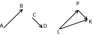
Figure 1.1. Adding equivalence classes of arrows.

Also arrow scalar multiplication is used to define a vector scalar multiplication as follows:

$$t\;[\overrightarrow{AB}]=_{V}[(t)\;\overrightarrow{AB}].$$

In Section 7 we prove that the set of equivalence classes of arrows, namely $\mathcal{P}_{v}$, with the operations of vector addition and vector scalar multiplication as defined above fulfills all the axioms of vector space. Then in Section 8 we demonstrate how the tools of this article can be applicable to the field of affine geometry by solving two problems through the context of the vector space $\mathcal{P}_{v}$ associated with the arrow space $\mathcal{P}_{A}$. The first problem is to show that for a given line $l_{OG}$, for every point $P\notin l_{OG}$, there exists a unique point $W\in l_{OG}$ such that $\left<\overrightarrow{WO},\overrightarrow{WP}\right>_{A}=0$; see Theorem 59. Then the Cauchy Schwartz inequality for arrows spaces is a corollary of Theorem 59. The other application is related to the barycentric coordinates of an affine space [[9], Page 22]. We show that given a set $\{P_{i}\}_{i=1}^{n}$ of distinct points in $\mathcal{P}$ and a finite set of real numbers $\{\lambda_{i}\}_{i=1}^{n}$ such that $\sum_{i=1}^{n}\lambda_{i}=1$, for a fixed coordinate free origin $O$, there exists a unique point $M$ such that $\sum_{i=1}^{n}[(\lambda_{i})\overrightarrow{OP_{i}}]=_{V}[\overrightarrow{OM}]$. Furthermore, the point $M$ is independent from the choice of the origin $O$.

2. Arrow Spaces

In this section we rigorously define the notion of an arrow and an arrow space. The definition of an arrow and its associated arrow space depends on a postulated set of points.

Axiom 0. There exists a set of points $\mathcal{P}$.

We will label individual points with Roman letters and with a slight abuse of notation denote $\mathcal{P}=\{A,\;B,\;C,...\}$. This labeling convention will allow us to denote equality among the elements of $\mathcal{P}$.

Definition 1.

Let $\mathcal{P}=\{A,\;B,\;C,...\}$ be a set of points. Let $A,\;B\in\mathcal{P}$. We define $A=_{P}B$ if and only if $A$ and $B$ refer to a single point. Otherwise, we write $A\neq_{P}B$ meaning that $A$ and $B$ refer to two distinct points.

We can now define an arrow as an ordered pair of points.

Definition 2.

Let $\mathcal{P}=\{A,\;B,\;C,...\}$ be a set of points. Let

$$\mathcal{P\times P}=\{(A,B)\;|\;A,\;B\in\mathcal{P}\}$$

be the Cartesian product of $\mathcal{P}$. Given any two points $A,\;B\in\mathcal{P}$, we define an arrow, denoted by $\overrightarrow{AB}$, to be the ordered pair $(A,B)$. The two points $A$ and $B$ are the tail and the head of the arrow $\overrightarrow{AB}$ respectively. If $A=_{P}B$, then $(A,B)=(A,A)$ and we denote the associated arrow by $\overrightarrow{AA}$. We call the set of all arrows, whose tails and heads are the points of a set $\mathcal{P}$, an arrow space and denote it by $\mathcal{P}_{A}$.

In the following definition we define equality among arrows.

Definition 3.

Let $\overrightarrow{AB},\;\overrightarrow{CD}$ be two arrows in $\mathcal{P}_{A}$. We put $\overrightarrow{AB}=_{A}\overrightarrow{CD}$ if and only if $A=_{P}C$ and $B=_{P}D$. If $A\neq_{P}C$ or $B\neq_{P}D$, we say that the two arrows are different and write $\overrightarrow{AB}\neq_{A}\overrightarrow{CD}$.

Next comes a technical definition, the negation of an arrow.

Definition 4.

Given the arrow $\overrightarrow{AB}$, we define $-\;\overrightarrow{AB}$ as $-\;\overrightarrow{AB}=\overrightarrow{BA}$; see Figure 3.1.

Note that if $A\neq_{P}B$, then $\overrightarrow{AB}\neq_{A}-\;\overrightarrow{AB}$.

In order to use arrows as a tool for solving various problems in affine geometry, and since arrows are actually precursors to vectors (see Section 6), we want to be able to manipulate them in a way that is reminiscent of the way we manipulate vectors. This means we need to define the binary operation of arrow addition and the notion of scalar multiplication acting on an arrow. Arrow addition is rather straightforward as seen by the following definition.

Definition 5.

Let $\overrightarrow{AB}$ and $\overrightarrow{BC}$ be any two arrows in $\mathcal{P}_{A}$. We define arrow addition, denoted by $+_{A}$, of $\overrightarrow{AB}$ and $\overrightarrow{BC}$ as $\overrightarrow{AB}+_{A}\overrightarrow{BC}=_{A}\overrightarrow{AC}$.

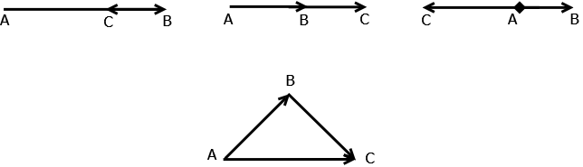
Figure 2.1. An illustration of Definition 5 where $\overrightarrow{AB}+_{A}\overrightarrow{BC}=_{A}\overrightarrow{AC}.$

However, to define the notion scalar multiplication in an arrow space we need metric notions of length and distance, along with the Euclidean notion of an angle. These crucial notions are algebraically captured by a postulated arrow pre-inner product, namely a symmetric, positive definite “bilinear” mapping $\left<-,-\right>_{A}:\mathcal{P}_{A}\times\mathcal{P}_{A}\longrightarrow\mathbb{R}$. This arrow pre-inner product will be a tool for defining the measure of an arrow, the definition of a line, and notion of betweenness for points that lie on a line.

Axiom 1. There exists a mapping $\left<-,-\right>_{A}:\mathcal{P}_{A}\times\mathcal{P}_{A}\longrightarrow\mathbb{R}$ such that

• (positive definiteness)

  (2.1) $$\left<\overrightarrow{AB},\overrightarrow{AB}\right>_{A}\geq 0\;\;\text{and}\;\left<\overrightarrow{AB},\overrightarrow{AB}\right>_{A}=0\;\text{if and only if}\;A=_{P}B,$$

• (symmetry)

  (2.2) $$\left<\overrightarrow{AB},\overrightarrow{CD}\right>_{A}=\left<\overrightarrow{CD},\overrightarrow{AB}\right>_{A},$$

• (arrow addition linearity)

  (2.3) $$\left<\overrightarrow{AB}+_{A}\overrightarrow{BC},\overrightarrow{LM}\right>_{A}=\left<\overrightarrow{AB},\overrightarrow{LM}\right>_{A}+\left<\overrightarrow{BC},\overrightarrow{MR}\right>_{A},$$

• (negation rule)

  (2.4) $$\left<-\;\overrightarrow{AB},\overrightarrow{CD}\right>_{A}=(-1)\;\left<\overrightarrow{AB},\overrightarrow{CD}\right>_{A}.$$

Regarding Axiom 1, we make two observations. First, Equation (2.2), when combined with Equation (2.3), implies that

$$\left<\overrightarrow{AB}+_{A}\overrightarrow{BC},\overrightarrow{LM}+_{A}\overrightarrow{MR}\right>_{A} =\left<\overrightarrow{AB},\overrightarrow{LM}\right>_{A}+\left<\overrightarrow{AB},\overrightarrow{MR}\right>_{A}$$

(2.5) $$+\left<\overrightarrow{BC},\overrightarrow{LM}\right>_{A}+\left<\overrightarrow{BC},\overrightarrow{MR}\right>_{A}.$$

Secondly, Equation (2.2), when combined with Equation (2.4), implies that

(2.6) $$\left<\overrightarrow{AB},-\;\overrightarrow{CD}\right>_{A}=(-1)\;\left<\overrightarrow{AB},\overrightarrow{CD}\right>_{A}=\left<-\;\overrightarrow{AB},\overrightarrow{CD}\right>_{A}.$$

Intuitively, we associate $\overrightarrow{AA}$ with the “zero” arrow, one of the infinitely many “zero” arrows. Thus we would like pre-inner product of Axiom 1 to behave correctly with respect to zero, namely that $\left<\overrightarrow{AA},-\right>=0$. This is indeed the case as evidenced by the following proposition.

Proposition 6.

For any two arrows $\overrightarrow{AA}$ and $\overrightarrow{CD}$ of $\mathcal{P}_{A}$, we have $\left<\overrightarrow{AA},\overrightarrow{CD}\right>_{A}=0$.

Proof.

Let $\overrightarrow{AA}$ and $\overrightarrow{CD}$ be any two arrows. Since

$$\overrightarrow{AA}=_{A}\overrightarrow{AD}+_{A}\overrightarrow{DA}\qquad\text{and}\qquad\;\overrightarrow{CD}=_{A}\overrightarrow{CA}+_{A}\overrightarrow{AD},$$

Definition 4 and Equations (2.5) and (2.6) imply that

$$\left<\overrightarrow{AA},\overrightarrow{CD}\right>_{A} =\left<\overrightarrow{AD}+_{A}\overrightarrow{DA},\overrightarrow{CA}+_{A}\overrightarrow{AD}\right>_{A}$$

$$=\left<\overrightarrow{AD},\overrightarrow{CA}\right>_{A}+\left<\overrightarrow{AD},\overrightarrow{AD}\right>_{A}+\left<\overrightarrow{DA},\overrightarrow{CA}\right>_{A}+\left<\overrightarrow{DA},\overrightarrow{AD}\right>_{A}$$

$$=\left<\overrightarrow{AD},\overrightarrow{CA}\right>_{A}+\left<\overrightarrow{AD},\overrightarrow{AD}\right>_{A}-\left<\overrightarrow{AD},\overrightarrow{CA}\right>_{A}-\left<\overrightarrow{AD},\overrightarrow{AD}\right>_{A}=0.$$

∎

The arrow pre-inner product of Axiom 1 provides a way of defining the measure (or length) of any arrow.

Definition 7.

For any arrow $\overrightarrow{AB}\in\mathcal{P}_{A}$, we define a measure, denoted $||-||_{A}$, as follows: $||\overrightarrow{AB}||_{A}=\sqrt{\left<\overrightarrow{AB},\overrightarrow{AB}\right>_{A}}$. If $||\overrightarrow{AB}||_{A}=1$, then we call this arrow a unit arrow.

The following lemma is an immediate consequence of Equation (2.1) and Definition 7.

Lemma 8.

For any arrow $\overrightarrow{AB}\in\mathcal{P}_{A}$, we have $||\overrightarrow{AB}||_{A}=0$ if and only if $A=_{P}B$.

We take advantage of the arrow pre-inner product and the measure to define the notion of scalar multiplication in an arrow space. To avoid confusion with the negation operation of Definition 4, we will always surround the scalar multiple with parenthesis.

Definition 9.

Let $\overrightarrow{AB}$ be any arrow in $\mathcal{P}_{A}$ and $t\in\mathbb{R}$. If $A=_{P}B$, or $t=0$, we put $(t)\overrightarrow{AB}=\overrightarrow{AA}$ . If $A\neq_{P}B$ and $t\neq 0$, we put $(t)\overrightarrow{AB}=_{A}\overrightarrow{AD}$, where $D$ is a point in $\mathcal{P}$ such that

• $||\overrightarrow{AD}||_{A}=|t|\;||\overrightarrow{AB}||_{A}$,
  

• $\left<\overrightarrow{AB},\overrightarrow{AD}\right>_{A}=||\overrightarrow{AB}||_{A}||\overrightarrow{AD}||_{A}$ if $t>0$,
  and $\left<\overrightarrow{AB},\overrightarrow{AD}\right>_{A}=-||\overrightarrow{AB}||_{A}||\overrightarrow{AD}||_{A}$ if $t<0$.

Observe that Definition 9 only deals with the existence of the point $D$. We will see in Section 5 that this $D$ is in fact unique; see Theorem 40.

The arrow pre-inner product, along with Definition 9 (2), suggests the following definition which is an algebraic quantification for when two arrow have the same direction.

Definition 10.

Let $A$, $B$, $C$, and $D$ be four distinct points of $\mathcal{P}$. We say $\overrightarrow{AB}$ has the same direction as $\overrightarrow{CD}$ if and only if $\left<\overrightarrow{AB},\overrightarrow{AD}\right>_{A}=||\overrightarrow{AB}||_{A}||\overrightarrow{AD}||_{A}$, or equivalently if and only if $\left<\frac{\overrightarrow{AB}}{|\overrightarrow{AB}||_{A}},\frac{\overrightarrow{CD}}{|\overrightarrow{CD}||_{A}}\right>=1$. We say $\overrightarrow{AB}$ has the opposite direction as $\overrightarrow{CD}$ if and only if $\left<\overrightarrow{AB},\overrightarrow{AD}\right>_{A}=-||\overrightarrow{AB}||_{A}||\overrightarrow{AD}||_{A}$, or equivalently if and only if $\left<\frac{\overrightarrow{AB}}{|\overrightarrow{AB}||_{A}},\frac{\overrightarrow{CD}}{|\overrightarrow{CD}||_{A}}\right>=-1$. Let $O$, $P$, $Q$, and $R$ be four (not necessarily distinct) points of $\mathcal{P}$. We say $\overrightarrow{OP}$ is perpendicular to, or forms a right angle with $\overrightarrow{QR}$ if and only if $\left<\overrightarrow{OP},\overrightarrow{QR}\right>_{A}=0$.

Remark 11.

Definition 10 implicitly measures when “angle” between two nontrivial arrows is zero (same direction), when it is $\pi$ (opposite direction), and when it is $\pi/2$ (right angle). These are the only three situations of angle measurement that are necessary for the axiomatic presentation of an arrow space presented in this paper. A thorough treatment of angles between two arrows is discussed in our LAA paper and in the Gingold/Salah paper.

Since we now have the notion of scalar multiplication, we require that the arrow pre-inner product of Axiom 1 behaves correctly with respect to this operation. In other words, we have the following axiom.

Axiom 2. (scalar multiplication linearity) For $\overrightarrow{AB}$ and $\overrightarrow{CD}$ any two arrows of $\mathcal{P}_{A}$ and $t\in\mathbb{R}$, we have

(2.7) $$\left<(t)\;\overrightarrow{AB},\overrightarrow{CD}\right>_{A}=t\left<\overrightarrow{AB},\overrightarrow{CD}\right>_{A}.$$

Observe that Equation (2.7), when combined with Equation (2.2), implies that

(2.8) $$\left<(t)\;\overrightarrow{AB},(s)\;\overrightarrow{CD}\right>_{A}=t\;s\left<\overrightarrow{AB},\overrightarrow{CD}\right>_{A},$$

a fact that will be extremely useful for the proofs in the paper.

The following lemma shows the relationship between length, scalar multiplication, and negation.

Lemma 12.

For any arrow $\overrightarrow{AB}\in\mathcal{P}_{A}$ and any $t\in\mathbb{R}$ we have

• (2.9) $$||(t)\;\overrightarrow{AB}||_{A}=|t|\;||\overrightarrow{AB}||_{A},$$

• (2.10) $$||\overrightarrow{AB}||_{A}=||\overrightarrow{BA}||_{A}.$$

Proof.

1) Definition 7 and Equation (2.8) imply that

$$||(t)\;\overrightarrow{AB}||_{A}^{2}=\left<(t)\;\overrightarrow{AB},(t)\;\overrightarrow{AB}\right>_{A}=t^{2}\left<\overrightarrow{AB},\overrightarrow{AB}\right>_{A}=t^{2}||\overrightarrow{AB}||_{A}^{2}.$$

Taking the positive square root of both sides preceding equation gives Equation (2.9).

2) Definitions 4 and 7, along with Equation (2.6), imply that

$$||\overrightarrow{BA}||_{A}^{2}=\left<\overrightarrow{BA},\overrightarrow{BA}\right>_{A}=\left<-\;\overrightarrow{AB},-\;\overrightarrow{AB}\right>_{A}=(-1)\;(-1)\left<\overrightarrow{AB},\overrightarrow{AB}\right>_{A}=||\overrightarrow{AB}||_{A}^{2}.$$

If we take the positive square root of both sides of the preceding equation we obtain Equation (2.10). ∎

We end this section with a theorem which relates scalar multiplication with equality of arrows.

Theorem 13.

Let $\overrightarrow{AB}$ be an arrow in $\mathcal{P}_{A}$ such that $A\neq_{P}B$. If $(a)\;\overrightarrow{AB}=_{A}(b)\;\overrightarrow{AB}$ for some real numbers $a$ and $b$, then we must have $a=b$.

Proof.

Let $\overrightarrow{AB}$ be an arrow such that $A\neq_{P}B$ and $(a)\;\overrightarrow{AB}=_{A}(b)\;\overrightarrow{AB}$ for some real numbers $a$ and $b$. If $a=0$, then it follows by Definition 9 that $(a)\;\overrightarrow{AB}=_{A}(0)\;\overrightarrow{AB}=_{A}\overrightarrow{AA}=(b)\;\overrightarrow{AB}$. Since $A\neq_{P}B$, it follows again by Definition 9 that $b=0$, which means that $a=b$. Now suppose that $a\neq 0$ and $b\neq 0$. Then Definition 7 implies that

(2.11) $$||(a)\;\overrightarrow{AB}||_{A}^{2}=\left<(a)\;\overrightarrow{AB},(a)\;\overrightarrow{AB}\right>_{A}.$$

Lemma 12 implies that $||(a)\;\overrightarrow{AB}||_{A}^{2}=|a|^{2}\;||\overrightarrow{AB}||_{A}^{2}$. Also, it is given that $(a)\;\overrightarrow{AB}=_{A}(b)\;\overrightarrow{AB}$. Thus, the Equation (2.11) can be rewritten as

$$|a|^{2}\;||\overrightarrow{AB}||_{A}^{2}=\left<(a)\;\overrightarrow{AB},(b)\;\overrightarrow{AB}\right>_{A}=ab\;\left<\overrightarrow{AB},\overrightarrow{AB}\right>_{A}.$$

where the last equality follows from by Equation (2.8). Since $\left<\overrightarrow{AB},\overrightarrow{AB}\right>_{A}=||\overrightarrow{AB}||_{A}^{2}$ (by Definition 7), the above equation implies that $|a|^{2}=a^{2}=ab$, or that $a=b$. ∎

3. How Arrows Differ From Vectors

For this section and the next we assume that we have an arrow space $\mathcal{P}_{A}$ and an arbitrary real vector space $V$. We want to examine the differences between $\mathcal{P}_{A}$ and $V$ and conclude that arrows are different entities than vectors. As a case in point, we show that arrow addition is restricted to certain pairs of arrows (the head of the first arrow must be the same as the tail of the second arrow) and cannot be performed on any two arbitrary arrows of $\mathcal{P}_{A}$; see Proposition 15. This is a fundamental difference from vector addition which is always defined for any two vectors in $V$. We also show in Proposition 16 that arrow addition is not commutative, a fact which draws a clear distinction between arrows and vectors. More differences between arrows and vectors will be further demonstrated.

We begin our analysis of the differences between arrows and vectors by recalling the well known fact that for any vector $v\in V$, it is always true that $(-1)\;v=-\;v$. However, this analog will not hold for arrows as witnessed by the fact that the two expressions $-\;\overrightarrow{AB}$ and $(-1)\;\overrightarrow{AB}$ in $\mathcal{P}_{A}$ are not the same.

Proposition 14.

For any $A\neq_{P}B$, we have $-\;\overrightarrow{AB}\neq_{A}(-1)\;\overrightarrow{AB}$.

Figure 3.1. An illustration of Proposition 14. Note that $(-1)\;\overrightarrow{AB}$ and $-\;\overrightarrow{AB}$ have different heads and tails.

Proof.

Definition 4 implies that $-\;\overrightarrow{AB}=_{A}\overrightarrow{BA}$, while Definition 9 implies that $(-1)\;\overrightarrow{AB}=_{A}\overrightarrow{AD}$, where $D\in\mathcal{P}$. Since $A\neq_{P}B$, an application of Definition 3 shows that $\overrightarrow{BA}\neq_{A}\overrightarrow{AD}$, which means that $-\;\overrightarrow{AB}\neq_{A}(-1)\;\overrightarrow{AB}$. ∎

Next we turn our attention to the ways in which arrow addition differs from that of vector addition. The addition of arrows, as given by Definition 5, seems natural. If we have an arrow $\overrightarrow{AB}$ which has $B$ as its head, and at the same time $B$ is the tail of another arrow $\overrightarrow{BC}$, then the resultant arrow obtained from adding these two arrows is the arrow that has its tail as the tail of the first arrow and its head as the head of the second arrow, namely $\overrightarrow{AC}$; see Figure 2.1. But this natural definition has some drawbacks. The first drawback is that arrow addition is not defined for arbitrary pairs of arrows.

Proposition 15.

The operation $+_{A}$ given by Definition 5 is not well defined for arbitrary elements of $\mathcal{P}_{A}\times\mathcal{P}_{A}$.

Proof.

This is an immediate consequence of Definition 5 since $\overrightarrow{AB}+_{A}\overrightarrow{DC}$ is not well defined if $B\neq_{P}D$. ∎

Proposition 15 demonstrates a fundamental difference between arrow addition and vector addition since vector addition is defined for any element of $V\times V$. Another fundamental difference between these two operations involves commutativity. Vector addition is commutative binary operation. However, this is surprisingly not the case for arrow addition as demonstrated by the following proposition. For this reason alone, arrows and vectors should not be thought of as a single notion.

Proposition 16.

The operation $+_{A}$ given by Definition 5 is not commutative.

Proof.

If $A$ and $B$ are two distinct points of $\mathcal{P}$, then Definition 5 implies that

$$\overrightarrow{AB}+_{A}\overrightarrow{BA}=_{A}\overrightarrow{AA}\qquad\text{and}\qquad\overrightarrow{BA}+_{A}\overrightarrow{AB}=_{A}\overrightarrow{BB}.$$

If $\overrightarrow{AB}+_{A}\overrightarrow{BA}=_{A}\overrightarrow{BA}+_{A}\overrightarrow{AB}$, then we would have $\overrightarrow{AA}=_{A}\overrightarrow{BB}$ which is impossible by Definition 3 as $A\neq_{P}B$. Therefore, $\overrightarrow{AB}+_{A}\overrightarrow{BA}\neq_{A}\overrightarrow{BA}+_{A}\overrightarrow{AB}$ implying that $+_{A}$ is noncommutative. ∎

We now turn our attention to differences between the corresponding operations of scalar multiplication. As was the case for arrow addition, we will discover that certain notions involving scalar multiplication in an arrow space are not well defined. First we show that the property $s(v+w)=sv+sw$, where $s\in\mathbb{R}$ and $v,w\in V$, does not necessarily hold in $\mathcal{P}_{A}$.

Theorem 17.

Let $A,\;B$, and $C$ be three distinct points of $\mathcal{P}$. Consider the two arrows $\overrightarrow{AB}$ and $\overrightarrow{BC}$ in $\mathcal{P}_{A}$. For any $s\neq 1$, $(s)\;(\overrightarrow{AB}+_{A}\overrightarrow{BC})$ and $(s)\;\overrightarrow{AB}+_{A}(s)\;\overrightarrow{BC}$ are not equivalent. In particular, $(s)\;\overrightarrow{AB}+_{A}(s)\;\overrightarrow{BC}$ is not well defined.

Proof.

First, if $s=0$, then Definitions 5 and 9 imply that

(3.1) $$(s)\;(\overrightarrow{AB}+_{A}\overrightarrow{BC})=_{A}(0)\;\overrightarrow{AC}=_{A}\overrightarrow{AA}.$$

On the other hand, let us “evaluate” expression $(s)\;\overrightarrow{AB}+_{A}(s)\;\overrightarrow{BC}$. Definition 9 implies that $(0)\;\overrightarrow{AB}=_{A}\overrightarrow{AA}$ and that $(0)\;\overrightarrow{BC}=_{A}\overrightarrow{BB}$. Since $A\neq_{P}B$, $\overrightarrow{AA}+_{A}\overrightarrow{BB}$ is not well defined in the sense of Definition 5.

Now assume $s\neq 0,\;1$. It follows by Definitions 5 and 9 that

(3.2) $$(s)\;(\overrightarrow{AB}+_{A}\overrightarrow{BC})=_{A}(s)\;\overrightarrow{AC}=_{A}\overrightarrow{AM},$$

for some points $C$ and $M$ in $\mathcal{P}$. On the other hand, Definition 9 implies that that $(s)\;\overrightarrow{AB}=_{A}\overrightarrow{AD}$ for some point $D$ in $\mathcal{P}$ with $D\neq_{P}B$ (as $s\neq 1$; see Theorem 23), and that $(s)\;\overrightarrow{BC}=_{A}\overrightarrow{BE}$ for some point $E$ in $\mathcal{P}$. Thus, $(s)\;\overrightarrow{AB}+_{A}(s)\;\overrightarrow{BC}=_{A}\overrightarrow{AD}+_{A}\overrightarrow{BE}$, and by Definition 5, as $D\neq_{P}B$, the right side is undefined. ∎

Next we show that the property $(s+t)v=sv+tv$, where $s,t\in\mathbb{R}$ and $v\in V$, also fails to hold in $\mathcal{P}_{A}$.

Theorem 18.

Given an arrow $\overrightarrow{AB}$ in $\mathcal{P}_{A}$ with $A\neq_{P}B$, let $s,\;t\in\mathbb{R}$ with $s\neq 0$. The two expressions $(s+t)\;(\overrightarrow{AB})$ and $(s)\;\overrightarrow{AB}+_{A}(t)\;\overrightarrow{AB}$ are not equivalent. However, if $s=0$, then $(s+t)\;(\overrightarrow{AB})=_{A}(s)\;\overrightarrow{AB}+_{A}(t)\;\overrightarrow{AB}$.

Proof.

First assume that $s=0$. Definition 9 implies that

(3.3) $$(t)\overrightarrow{AB}=_{A}\overrightarrow{AD}$$

for some point $D$ in $\mathcal{P}$ and that

(3.4) $$(s)\overrightarrow{AB}=_{A}\overrightarrow{AA}.$$

Equations (3.3) and (3.4), along with Definition 5, imply that implies that

$$(s+t)\;(\overrightarrow{AB})=_{A}(t)\overrightarrow{AB}=_{A}\overrightarrow{AD}=_{A}\overrightarrow{AA}+_{A}\overrightarrow{AD}=(s)\;(\overrightarrow{AB})+_{A}(t)\overrightarrow{AB}.$$

Now suppose that $s\neq 0$ and let $(s)\overrightarrow{AB}=_{A}\overrightarrow{AC}$ and $(t)\;\overrightarrow{AB}=_{A}\overrightarrow{AD}$ for some points $C$ and $D$ in $\mathcal{P}$, with $C\neq_{P}A$. The right hand side of the expression

(3.5) $$(s)\overrightarrow{AB}+_{A}(t)\overrightarrow{AB}=_{A}\overrightarrow{AC}+_{A}\overrightarrow{AD},$$

is undefined according to Definition 5. On the other hand, if we put $s+t=r$ for some real number $r$, then Definition 9 implies that

(3.6) $$(s+t)\;(\overrightarrow{AB})=_{A}(r)\overrightarrow{AB}=_{A}\overrightarrow{AE},$$

where $E$ is a point in $\mathcal{P}$. Thus the expression in Equation (3.6) is well defined while the right hand side of the Equation (3.5) is not well defined which makes it impossible to compare the two left hand sides of these equations. ∎

Corollary 19.

For any arrow $\overrightarrow{AB}$ in $\mathcal{P}_{A}$ with $A\neq_{P}B$, $\overrightarrow{AB}+_{A}(-1)\;\overrightarrow{AB}$ is not well defined.

4. Similarities Between Arrow Spaces and Vector Spaces

So far we have investigated some axioms of vector space $V$ which do not hold in $\mathcal{P}_{A}$. In this section we turn our attention to those axioms of $V$ which have corresponding analogs in $\mathcal{P}_{A}$. We first show that arrow addition $+_{A}$ is associative.

Theorem 20.

Let $\overrightarrow{AB},\;\overrightarrow{BC},\;\overrightarrow{CD}$ be arrows in $\mathcal{P}_{A}$. Then

$$(\overrightarrow{AB}+_{A}\overrightarrow{BC})+_{A}\overrightarrow{CD}=_{A}\overrightarrow{AB}+_{A}(\overrightarrow{BC}+_{A}\overrightarrow{CD}),$$

that is the addition $+_{A}$ is associative.

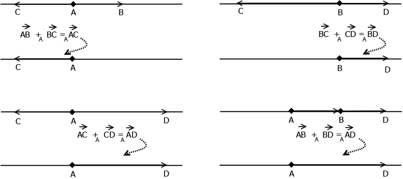
Figure 4.1. An illustration of Theorem 20. The left section of this figure explains $(\overrightarrow{AB}+_{A}\overrightarrow{BC})+_{A}\overrightarrow{CD}$, while the right one stands for $\overrightarrow{AB}+_{A}(\overrightarrow{BC}+_{A}\overrightarrow{CD})$.

Proof.

Given three arrows $\overrightarrow{AB},\;\overrightarrow{BC}$, and $\overrightarrow{CD}$ in $\mathcal{P}_{A}$, Definition 5 implies that

(4.1) $$(\overrightarrow{AB}+_{A}\overrightarrow{BC})+_{A}\overrightarrow{CD}=_{A}\overrightarrow{AC}+_{A}\overrightarrow{CD}=_{A}\overrightarrow{AD}.$$

A similar calculation shows that

$$\overrightarrow{AB}+_{A}(\overrightarrow{BC}+_{A}\overrightarrow{CD})=_{A}\overrightarrow{AB}+_{A}\overrightarrow{BD}\\ =_{A}\overrightarrow{AD}.$$

Combining the Equations (4.1) and (4) finishes the proof. ∎

A similar result regarding occurs for arrow scalar multiplication. But in order to prove the associativity of arrow scalar multiplication we will need the following proposition. This proposition is important in its own right since it will be crucial to proving the existence of line between any two points; see Subsection 5.1.

Proposition 21.

Let $\overrightarrow{AB}$ and $\overrightarrow{AD}$ be two arrows of $\mathcal{P}_{A}$ such that $||\overrightarrow{AB}||_{A}=||\overrightarrow{AD}||_{A}$ and $\frac{\left<\overrightarrow{AB},\overrightarrow{AD}\right>_{A}}{||\overrightarrow{AB}||_{A}\;||\overrightarrow{AD}||_{A}}=1$. Then $B=_{P}D$.

Proof.

Assume by way of contradiction that $B\neq_{P}D$. By hypothesis we have $||\overrightarrow{AB}||_{A}=||\overrightarrow{AD}||_{A}$ and $\frac{\left<\overrightarrow{AB},\overrightarrow{AD}\right>_{A}}{||\overrightarrow{AB}||_{A}\;||\overrightarrow{AD}||_{A}}=1$, which implies that

(4.2) $$\left<\overrightarrow{AB},\overrightarrow{AD}\right>_{A}=\left<\overrightarrow{AD},\overrightarrow{AD}\right>_{A}.$$

An application of Axiom 1 and Definition 4 to Equation (4.2) yields

$$\left<\overrightarrow{DA},\overrightarrow{AD}\right>_{A}+\left<\overrightarrow{AB},\overrightarrow{AD}\right>_{A}=\left<\overrightarrow{DB},\overrightarrow{AD}\right>_{A}=0.$$

Since $\overrightarrow{AD}=_{A}-\overrightarrow{DA}$ (see Definition 4), the preceding equation is equivalent to

(4.3) $$\left<\overrightarrow{DB},\overrightarrow{DA}\right>_{A}=0.$$

On the other hand, since $||\overrightarrow{AB}||_{A}=||\overrightarrow{AD}||_{A}$ we can rewrite Equation (4.2) as $\left<\overrightarrow{AB},\overrightarrow{AD}\right>_{A}=\left<\overrightarrow{AB},\overrightarrow{AB}\right>_{A}$. Then a similar argument shows that

(4.4) $$\left<\overrightarrow{DB},\overrightarrow{AB}\right>_{A}=0.$$

Adding Equations (4.3) and (4.4) and using Axiom 1 gives us

(4.5) $$\left<\overrightarrow{DB},\overrightarrow{DA}\right>_{A}+\left<\overrightarrow{DB},\overrightarrow{AB}\right>_{A}=\left<\overrightarrow{DB},\overrightarrow{DB}\right>_{A}=0.$$

By Definition 7, Equation (4.5) means that $||\overrightarrow{DB}||_{A}^{2}=0$, that is $||\overrightarrow{DB}||_{A}=0$. But by Lemma 8, the equation $||\overrightarrow{DB}||_{A}=0$ implies that $D=_{P}B$ which contradicts our assumption that $B\neq_{P}D$. Thus we conclude that $B=_{P}D$. ∎

Theorem 22.

For any $s,\;t\in\mathbb{R}$ and any arrow $\overrightarrow{AB}$ in $\mathcal{P}_{A}$, $(s\;t)\overrightarrow{AB}=_{A}(s)((t)\;\overrightarrow{AB})$, that is the arrow scalar multiplication is associative.

Proof.

If $A=_{P}B$ or at least one of the real numbers $s$ or $t$ is zero, then it follows directly from Definition 9 that $(st)\;\overrightarrow{AB}=_{A}(s)\;((t)\;\overrightarrow{AB})=_{A}\overrightarrow{AA}.$ Now let us assume $A\neq_{P}B$ and $s,t\neq 0$. Let

(4.6) $$(t)\;\overrightarrow{AB}=_{A}\overrightarrow{AC},$$

(4.7) $$(s)\;((t)\;\overrightarrow{AB})=_{A}(s)\;\overrightarrow{AC}=_{A}\overrightarrow{AD},$$

and

(4.8) $$(s\;t)\;\overrightarrow{AB}=_{A}\overrightarrow{AF},$$

for some points $C,\;D$, and $F$ in $\mathcal{P}$. We want to show that $\overrightarrow{AD}=_{A}\overrightarrow{AF}$. By Definition 9 and Equations (4.6) and (4.7) we have

$$||\overrightarrow{AC}||_{A}=|t|\;||\overrightarrow{AB}||_{A},\qquad||\overrightarrow{AD}||_{A}=|s|\;||\overrightarrow{AC}||_{A},$$

which implies that

(4.9) $$||\overrightarrow{AD}||_{A}=|s\;t|\;||\overrightarrow{AB}||_{A}.$$

Also, Definition 9 and Equation (4.8) imply that

(4.10) $$||\overrightarrow{AF}||_{A}=|s\;t|\;||\;\overrightarrow{AB}||_{A}.$$

We get from Equations (4.9) and (4.10) that

(4.11) $$||\overrightarrow{AF}||_{A}=||\overrightarrow{AD}||_{A}.$$

Next we show that $\left<\frac{\overrightarrow{AD}}{||\overrightarrow{AD}||_{A}},\frac{\overrightarrow{AF}}{||\overrightarrow{AF}||_{A}}\right>_{A}=1$. By Equations (4.7) and (4.8), and since $||\overrightarrow{AF}||_{A}=||\overrightarrow{AD}||_{A}=|s\;t|\;||\overrightarrow{AB}||_{A}$, we have

$$\left<\frac{\overrightarrow{AD}}{||\overrightarrow{AD}||_{A}},\frac{\overrightarrow{AF}}{||\overrightarrow{AF}||_{A}}\right>_{A}=\left<\frac{s\;((t)\;\overrightarrow{AB})}{|s\;t|\;||\overrightarrow{AB}||_{A}},\frac{(s\;t)\;\overrightarrow{AB}}{|s\;t|\;||\overrightarrow{AB}||_{A}}\right>_{A}.$$

Using Equation (2.8) and Definition 7, the preceding equation simplifies to

(4.12) $$\left<\frac{\overrightarrow{AD}}{||\overrightarrow{AD}||_{A}},\frac{\overrightarrow{AF}}{||\overrightarrow{AF}||_{A}}\right>_{A}=\frac{(s\;t)^{2}\;\left<\overrightarrow{AB},\overrightarrow{AB}\right>_{A}}{|s\;t|^{2}\;||\overrightarrow{AB}||_{A}^{2}}=1,$$

Then Proposition 21 implies that $D=_{P}F$ as desired. ∎

Recall that vector space $V$ has a unique vector $0$ which is the identity element with respect to addition, i.e. $v+0=v=0+v=v$ for all $v\in V$. If we think of $\overrightarrow{AA}$ as an analog to the zero vector, then the following theorem implies that $\overrightarrow{AA}$ is a left additive identity for arrows that have the point $A$ as a tail.

Theorem 23.

Given an arrow $\overrightarrow{AB}$ of $\mathcal{P}_{A}$, there is a a unique arrow $\overrightarrow{AA}$ (similarly, a unique arrow $\overrightarrow{BB}$) such that

(4.13) $$\overrightarrow{AA}+_{A}\overrightarrow{AB}=_{A}\overrightarrow{AB},$$

(and similarly $\overrightarrow{AB}+_{A}\overrightarrow{BB}=_{A}\overrightarrow{AB}$).

Proof.

Let $\overrightarrow{AB}$ be an arrow in $\mathcal{P}_{A}$. Since $\overrightarrow{AA}$ is well defined by Definition 2, Definition 5 implies that $\overrightarrow{AA}+_{A}\overrightarrow{AB}=_{A}\overrightarrow{AB}.$ Now if there exists another arrow $\overrightarrow{CD}$ such that

(4.14) $$\overrightarrow{CD}+_{A}\overrightarrow{AB}=_{A}\overrightarrow{AB},$$

then since $\overrightarrow{AB}$ is fixed, Definition 5 implies that $D=_{P}A$. Thus Equation (4.14) becomes

(4.15) $$\overrightarrow{CA}+_{A}\overrightarrow{AB}=_{A}\overrightarrow{CB}.$$

Since Equations (4.14) and (4.15) are equivalent, comparing them yields $\overrightarrow{CB}=_{A}\overrightarrow{AB}$, which means (by Definition 3) that we must have $C=_{P}A$. Therefore, $\overrightarrow{CD}=_{A}\overrightarrow{AA}$. ∎

For any $v\in V$, there is a unique element $-v$ (the additive inverse of $v$) such that $v+(-v)=-v+v=0$. The following theorem is the arrow space analog of the additive inverse.

Theorem 24.

Let $\overrightarrow{AA}$ be fixed in $\mathcal{P}_{A}$. For any arrow $\overrightarrow{AB}$ in $\mathcal{P}_{A}$ there exists a unique arrow $\overrightarrow{BA}$ such that

(4.16) $$\overrightarrow{AB}+_{A}\overrightarrow{BA}=_{A}\overrightarrow{AA}.$$

.

Proof.

Let $\overrightarrow{AA}$ be fixed. For any point $B\in\mathcal{P}$, $\overrightarrow{AB}$ is in $\mathcal{P}_{A}$. By Definition 2, $\overrightarrow{BA}$ is also in $\mathcal{P}_{A}$, and Definition 5 implies that

$$\overrightarrow{AB}+_{A}\overrightarrow{BA}=_{A}\overrightarrow{AA}.$$

Now if exists another arrow $\overrightarrow{CD}$ such that

(4.17) $$\overrightarrow{AB}+_{A}\overrightarrow{CD}=_{A}\overrightarrow{AA},$$

then since $\overrightarrow{AB}$ is fixed, the only way for $\overrightarrow{AB}+_{A}\overrightarrow{CD}$ to be defined is to have $C=_{P}B$. Thus if we change $C$ into $B$ in the Equation (4.17) and use Definition 5, we would have

(4.18) $$\overrightarrow{AB}+_{A}\overrightarrow{BD}=_{A}\overrightarrow{AD}.$$

Since Equations (4.17) and (4.18) are equivalent, comparing them yields $\overrightarrow{AD}=_{A}\overrightarrow{AA}$ which means ( by Definition 3), that $D=_{P}A$. Thus, $\overrightarrow{CD}=_{A}\overrightarrow{BA}$. ∎

The following proposition, the arrows space analog of the vector space property $s0=0$, is a direct consequence of Definition 9.

Proposition 25.

For any arrow $\overrightarrow{AA}$ in $\mathcal{P}_{A}$ and any $s\in\mathbb{R}$, $(s)\overrightarrow{AA}=_{A}\overrightarrow{AA}$.

In a vector space $V$, given $v\in V$, there is a unique scalar, denoted $1$, such that $1v=v$. The scalar multiplication identity in an arrow space $\mathcal{P}_{A}$ can also be identified as follows.

Theorem 26.

For any arrow $\overrightarrow{AB}$ in an arrow space $\mathcal{P}_{A}$, $(1)\overrightarrow{AB}=_{A}\overrightarrow{AB}$.

Proof.

If $A=_{P}B$, then the result follows from Proposition 25. So assume $A\neq_{P}B$. Lemma 8 implies that $||\overrightarrow{AB}||_{A}\neq 0$. Definition 9 implies that $(1)\overrightarrow{AB}=\overrightarrow{AD}$ for some point $D$ such that

(4.19) $$||\overrightarrow{AD}||=||(1)\overrightarrow{AB}||_{A}=||\overrightarrow{AB}||_{A},$$

and

(4.20) $$\left<\frac{\overrightarrow{AD}}{||\overrightarrow{AD}||},\;\frac{\overrightarrow{AB}}{||\overrightarrow{AB}||_{A}}\right>_{A}=1.$$

From Equations (4.19), and (4.20) we would like to conclude that $D=_{P}B$. But this will follow from the uniqueness of the point $D$ as referenced by the remark that followed Definition 9. ∎

In a vector space $V$, multiplication by the scalar $0$ always returns the zero vector, i.e. $0v=0$ for any $v\in V$. We end this section with the following proposition which provides the arrow space analog, where arrows of the form $\overrightarrow{AA}$ correspond to the zero vector.

Proposition 27.

For any arrow $\overrightarrow{AB}$ in $\mathcal{P}_{A}$, $(0)\overrightarrow{AB}=_{A}\overrightarrow{AA}$.

Proof.

Let $\overrightarrow{AB}$ be an arrow in $\mathcal{P}_{A}$. By Definition 9, $(0)\;\overrightarrow{AB}=_{A}\overrightarrow{AA}$. ∎

5. Lines in an Arrow Space

The line is a crucial concept of Euclidean geometry since it appears within three of Euclid’s original five axioms. Because an arrow space is to be the precursor of the Euclidean plane reinterpreted as a two-dimensional vector space, we will need to define what is meant by a line $l$ within an abstract arrow space $\mathcal{P}_{A}$. For any fixed $\overrightarrow{AB}\in\mathcal{P}_{A}$, we can use scalar multiplication to define a set of points with $\mathcal{P}_{A}$ determined by the “direction” of $\overrightarrow{AB}$. This aforementioned set of points in $\mathcal{P}_{A}$ is the line $l$. This set of points on $l$, namely $\mathcal{P}_{l}$, gives rise to a one-dimensional arrow space $\mathcal{P}_{l_{A}}$ contained within $\mathcal{P}_{A}$. When considered as an independent arrow space apart from $\mathcal{P}_{A}$, the arrow space $\mathcal{P}_{l_{A}}$ has the property that parallel postulate of the Euclidean plane is no longer an axiom but a theorem; see Subsection 5.3. This surprising result justifies an analysis of $\mathcal{P}_{l_{A}}$ in its own right and is focus of the two subsections contained within this section. But all of this analysis hinges on the definition and existence of a line within an arrow space. Thus we begin with this pivotal definition.

Definition 28.

Let $\mathcal{P}_{A}$ be a given arrow space. Given a fixed point $A\in\mathcal{P}$ and an arrow $\overrightarrow{AB}\in\mathcal{P}_{A}$ with $A\neq_{P}B$, a line containing $A$ and $B$, denoted by $l_{AB}$ or $l$, is the set of all the heads of arrows $\overrightarrow{AC}$ such that there exists $t\in\mathbb{R}$ with $\overrightarrow{AC}=_{A}(t)\;\overrightarrow{AB}$. The set of points on Line $l$ is denoted by $\mathcal{P}_{l_{AB}}$ or $\mathcal{P}_{l}$ when $\overrightarrow{AB}$ is understood. The set of arrows determined by $\mathcal{P}_{l}$ is the arrow space $\mathcal{P}_{l_{A}}$.

To justify the existence of a line between any two distinct points $A$ and $B$ of $\mathcal{P}$, we consider the next axiom which matches points on a line with the real numbers.

Axiom 3. Let $l$ be a line containing the points $A$ and $B$. There exists a one-to-one correspondence between the set of real numbers and the set of points that lie on $l$.

Axiom 3 shows that Line $l_{AB}$ is a nonempty set of $\mathcal{P}$; see the proof of Theorem 33. Furthermore, since the real line is a totally ordered set, Axiom 3 provides a geometric intuition of order (or betweenness) of points in $\mathcal{P}_{l}$ associated with Line $l$. The official algebraic definition of this geometric intuition is provided below.

Definition 29.

Let $A,\;B$, and $C$ be any three distinct points on Line $l$. We say that the point $B$ is between $A$ and $C$ if $\left<\frac{\overrightarrow{BA}}{||\overrightarrow{BA}||_{A}},\frac{\overrightarrow{BC}}{||\overrightarrow{BC}||_{A}}\right>_{A}=-1$. If $B$ is between $A$ and $C$, we write $A\prec B\prec C$.

Figure 5.1. A depiction of $A\prec B\prec C$, where $A$, $B$, and $C$ are three points on Line $l$.

The notion of betweenness provided by Definition 29, along with the correspondence between the real line and the line $l$ determined by $\overrightarrow{AB}$, allows us to illustrate an abstract arrow $\overrightarrow{AB}$ as a directed finite line segment which starts at the Tail $A$ and ends at Head $B$, where the direction is recorded by the placement of an arrowhead on the head point $B$. We have been using this illustration convention throughout the previous sections even though we had no concept of betweenness and an arrow $\overrightarrow{AB}$, in all rigor, should have been depicted as two discrete points $A$ and $B$.

5.1. Existence of Line

We are interested in proving an arrow space analog of Euclid’s first axiom, namely that given any two distinct points, there exists a unique line which contains the two given points; see Theorem 33. Before we do this, we introduce a lemma which is used in the proof of Theorem 33. This lemma provides an arrow pre-inner product constraint for two unit arrows which lie on the same line, namely that the unit arrows have the same direction (pre-inner product is $1$) or that the unit arrows have opposite directions (pre-inner product is $-1$).

Lemma 30.

If $A$, $B$, $M$, and $L$ are four distinct points of Line $l_{AB}$, then

(5.1) $$\frac{\left<\overrightarrow{ML},\overrightarrow{AB}\right>_{A}}{||\overrightarrow{ML}||_{A}\;||\overrightarrow{AB}||_{A}}=\pm 1.$$

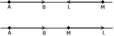
Figure 5.2. Points on Line $l_{AB}$ illustrating Equation (5.1).

Proof.

Let $A$, $B$, $M$, and $L$ be four distinct points of line $l_{AB}$. By Definition 28 there exists $t_{M},\;t_{L}\in\mathbb{R}$ such that

(5.2) $$\overrightarrow{AM}=_{A}(t_{M})\overrightarrow{AB},\qquad\overrightarrow{AL}=_{A}(t_{L})\overrightarrow{AB},$$

which when combined with Definition 4 implies that

(5.3) $$\overrightarrow{MA}=_{A}-((t_{M})\overrightarrow{AB}).$$

Since $\overrightarrow{MA}+_{A}\overrightarrow{AL}=_{A}\overrightarrow{ML}$, we find through various applications of Axioms 1 and 2 that

(5.4) $$\frac{\left<\overrightarrow{ML},\overrightarrow{AB}\right>_{A}}{||\overrightarrow{ML}||_{A}\;||\overrightarrow{AB}||_{A}}=\frac{(-t_{M}+t_{L})\left<\overrightarrow{AB},\overrightarrow{AB}\right>_{A}}{||\overrightarrow{MA}+_{A}\overrightarrow{AL}||_{A}\;||\overrightarrow{AB}||_{A}}.$$

We can also simplify the denominator of Equation (5.4) in a similar manner, namely

(5.5) $$||\overrightarrow{MA}+_{A}\overrightarrow{AL}||_{A}=\sqrt{(t_{L}-t_{M})^{2}}\;||\overrightarrow{AB}||_{A}.$$

Equation (5.5) implies that

(5.6) $$||\overrightarrow{MA}+_{A}\overrightarrow{AL}||_{A}\;||\overrightarrow{AB}||_{A}=|t_{L}-t_{M}|\;||\overrightarrow{AB}||_{A}^{2}.$$

Plugging the result of Equation (5.6), (notice that $t_{L}-t_{M}\neq 0$ since otherwise we would have $L=_{P}M$ which is a contradiction to the hypotheses of this lemma), into the right hand side of the Equation (5.4) yields

$$\frac{\left<\overrightarrow{ML},\overrightarrow{AB}\right>_{A}}{||\overrightarrow{ML}||_{A}\;||\overrightarrow{AB}||_{A}}=\frac{(t_{L}-t_{M})\;||\overrightarrow{AB}||_{A}^{2}}{|t_{L}-t_{M}|\;||\overrightarrow{AB}||_{A}^{2}}=\pm 1.$$

∎

We next provide a pre-inner product condition for determining when a given point lies on a fixed line; see Theorems 31 and 32. Since the set of points $\mathcal{P}_{l}$ of $l_{AB}$ is contained within underlying the set of points $\mathcal{P}$ of $\mathcal{P}_{A}$, we can examine the following situation. Suppose for some point $D\in\mathcal{P}$ distinct from $A$ and $B$, we have $\frac{\left<\overrightarrow{AB},\overrightarrow{AD}\right>_{A}}{||\overrightarrow{AB}||_{A}\;||\overrightarrow{AD}||_{A}}=1$, then $D\in\mathcal{P}_{l}$, see Figure 5.2.

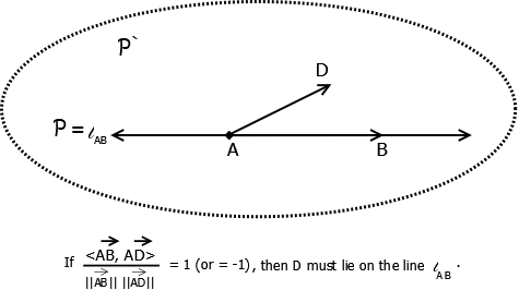
Figure 5.3. An illustration for when a given point lies on a fixed line.

Theorem 31.

Let $A,\;B,\;D$ be three distinct points of $\mathcal{P}$ such that $\frac{\left<\overrightarrow{AB},\overrightarrow{AD}\right>_{A}}{||\overrightarrow{AB}||_{A}\;||\overrightarrow{AD}||_{A}}=1$. Then the following is true:

• $$\frac{\left<\overrightarrow{AB},\overrightarrow{BD}\right>}{||\overrightarrow{AB}||_{A}\;||\overrightarrow{BD}||_{A}}=\pm 1;$$

• either

  $$||\overrightarrow{AD}||_{A}=||\overrightarrow{AB}||_{A}+||\overrightarrow{BD}||_{A},$$

  

  Figure 5.4. A depiction of three points $A,\;B,\;D$ where $||\overrightarrow{AD}||_{A}=||\overrightarrow{AB}||_{A}+||\overrightarrow{BD}||_{A}$.

  or

  $$||\overrightarrow{AB}||_{A}=||\overrightarrow{AD}||_{A}+||\overrightarrow{DB}||_{A};$$

  

  Figure 5.5. A depiction of three points $A,\;B,\;D$ when $||\overrightarrow{AB}||_{A}=||\overrightarrow{AD}||_{A}+||\overrightarrow{DB}||_{A}$.

• there exists $t_{D}\in\mathbb{R}$ with $t_{D}>0$ such that $\overrightarrow{AD}=_{A}(t_{D})\overrightarrow{AB}$; thus the point $D$ lies on the line $l_{AB}$; see Figure 5.4.

Proof.

1) First notice that it is not given that $A,\;B$, and $D$ lie on the same line; in fact, we need to prove this. So let $A,\;B$, and $D$ be three distinct points of $\mathcal{P}$ such that

(5.7) $$\frac{\left<\overrightarrow{AB},\overrightarrow{AD}\right>_{A}}{||\overrightarrow{AB}||_{A}\;||\overrightarrow{AD}||_{A}}=1,$$

Since $\overrightarrow{AD}=_{A}\overrightarrow{AB}+_{A}\overrightarrow{BD}$, applications of Axiom 1 and Definition 7 to Equation (5.7) implies that

$$1=\frac{\left<\overrightarrow{AB},\overrightarrow{AB}+_{A}\overrightarrow{BD}\right>_{A}}{||\overrightarrow{AB}||_{A}\;||\overrightarrow{AD}||_{A}}\ =\frac{||\overrightarrow{AB}||_{A}^{2}+\left<\overrightarrow{AB},\overrightarrow{BD}\right>_{A}}{||\overrightarrow{AB}||_{A}\;||\overrightarrow{AD}||_{A}}.$$

Multiplying both sides in the above by $||\overrightarrow{AB}||_{A}\;||\overrightarrow{AD}||_{A}$ yields

(5.8) $$||\overrightarrow{AB}||_{A}^{2}+\left<\overrightarrow{AB},\overrightarrow{BD}\right>_{A}=||\overrightarrow{AB}||_{A}\;||\overrightarrow{AD}||_{A}.$$

Similar calculations show that

(5.9) $$||\overrightarrow{AD}||_{A}=\sqrt{||\overrightarrow{AB}||_{A}^{2}+2\left<\overrightarrow{AB},\overrightarrow{BD}\right>_{A}+||\overrightarrow{BD}||_{A}^{2}}.$$

If we combine Equations (5.8) and (5.9), we get

(5.10) $$||\overrightarrow{AB}||_{A}^{2}+\left<\overrightarrow{AB},\overrightarrow{BD}\right>_{A}=||\overrightarrow{AB}||_{A}\;\sqrt{||\overrightarrow{AB}||_{A}^{2}+2\left<\overrightarrow{AB},\overrightarrow{BD}\right>_{A}+||\overrightarrow{BD}||_{A}^{2}}.$$

By squaring both sides of the above, we get

$$||\overrightarrow{AB}||_{A}^{4} +2||\overrightarrow{AB}||_{A}^{2}\;\left<\overrightarrow{AB},\overrightarrow{BD}\right>_{A}+\left<\overrightarrow{AB},\overrightarrow{BD}\right>^{2}$$

$$=||\overrightarrow{AB}||_{A}^{4}+2||\overrightarrow{AB}||_{A}^{2}\;\left<\overrightarrow{AB},\overrightarrow{BD}\right>_{A}+||\overrightarrow{AB}||_{A}^{2}\;||\overrightarrow{BD}||_{A}^{2},$$

which is equivalent to

$$\left<\overrightarrow{AB},\overrightarrow{BD}\right>^{2}=||\overrightarrow{AB}||_{A}^{2}\;||\overrightarrow{BD}||_{A}^{2}.$$

Taking the square root of both sides of the above gives

(5.11) $$\left<\overrightarrow{AB},\overrightarrow{BD}\right>=\pm||\overrightarrow{AB}||_{A}\;||\overrightarrow{BD}||_{A}.$$

Since $A\neq_{P}B,\;B\neq_{P}D$, it follows by Lemma 8 that $||\overrightarrow{AB}||_{A}\neq 0$ and that $||\overrightarrow{BD}||_{A}\neq 0$. Hence, if we divide both sides of the Equation (5.11) by $||\overrightarrow{AB}||_{A}\;||\overrightarrow{BD}||_{A}$, we get the desired equation.

2) To prove the second part of the theorem we return to Equation (5.7) and work on expanding the numerator $\left<\overrightarrow{AB},\overrightarrow{AD}\right>_{A}$ via Axiom 1 and the fact that $\overrightarrow{AD}=_{A}\overrightarrow{AB}+_{A}\overrightarrow{BD}$ and $\overrightarrow{AB}=_{A}\overrightarrow{AD}+_{A}\overrightarrow{DB}$. Equation (5.7) may then be rewritten as

$$||\overrightarrow{AB}||_{A}\;||\overrightarrow{AD}||_{A} =\left<\overrightarrow{AB},\overrightarrow{AD}\right>_{A}=\left<\overrightarrow{AD}+_{A}\overrightarrow{DB},\overrightarrow{AD}\right>_{A}$$

$$=\left<\overrightarrow{AD},\overrightarrow{AD}\right>_{A}+\left<\overrightarrow{DB},\overrightarrow{AD}\right>_{A}=\left<\overrightarrow{AD},\overrightarrow{AD}\right>_{A}+\left<\overrightarrow{DB},\overrightarrow{AB}+\overrightarrow{BD}\right>_{A}$$

(5.12) $$=||\overrightarrow{AD}||_{A}^{2}+\left<\overrightarrow{DB},\overrightarrow{AB}\right>_{A}-||\overrightarrow{BD}||_{A}^{2}.$$

The next step is to manipulate Equation (5.11) through Definition 4 and repeated applications of Axiom 1. Definition 4 implies that $\overrightarrow{BD}=_{A}-\overrightarrow{DB}$. Thus, it follows by Equation (2.6) and Equation (2.2) that

$$\left<\overrightarrow{AB},\overrightarrow{BD}\right>=\left<\overrightarrow{BD},\overrightarrow{AB}\right>=-\left<\overrightarrow{AB},\overrightarrow{DB}\right>.$$

This means that we can rewrite Equation (5.11) (noticing that $||\overrightarrow{DB}||_{A}=||\overrightarrow{BD}||_{A}$ by Equation (2.10)) as follows

(5.13) $$\left<\overrightarrow{DB},\overrightarrow{AB}\right>=\mp||\overrightarrow{AB}||_{A}\;||\overrightarrow{DB}||_{A}.$$

If we combine Equations (5.12) and (5.13), we get

$$||\overrightarrow{AD}||_{A}^{2}\mp||\overrightarrow{AB}||_{A}\;||\overrightarrow{DB}||_{A}-||\overrightarrow{DB}||_{A}^{2}=||\overrightarrow{AB}||_{A}\;||\overrightarrow{AD}||_{A}.$$

Rearranging the above equation yields

$$||\overrightarrow{AD}||_{A}^{2}-||\overrightarrow{DB}||_{A}^{2}=||\overrightarrow{AB}||_{A}\;||\overrightarrow{AD}||_{A}\pm||\overrightarrow{AB}||_{A}\;||\overrightarrow{DB}||_{A},$$

that is,

(5.14) $$(||\overrightarrow{AD}||_{A}-||\overrightarrow{DB}||_{A})(||\overrightarrow{AD}||_{A}+||\overrightarrow{DB}||_{A})=||\overrightarrow{AB}||_{A}\;(||\overrightarrow{AD}||_{A}\pm||\overrightarrow{DB}||_{A}).$$

Now Equation (5.14) tells us that either

(5.15) $$||\overrightarrow{AD}||_{A}-||\overrightarrow{BD}||_{A} =||\overrightarrow{AB}||_{A},\qquad\text{or}$$

(5.16) $$||\overrightarrow{AD}||_{A}+||\overrightarrow{DB}||_{A} =||\overrightarrow{AB}||_{A},$$

as desired.

3) Notice that when proving Part 2 either Equation (5.15) or Equation (5.16), is valid. We will show the validity of Equation (5.15) being valid and leave the validity of Equation (5.16) to the reader. Since $A\neq_{P}B$, Lemma 8 implies that $||\overrightarrow{AB}||_{A}\neq 0$. Hence, Equation becomes (5.15) as $||\overrightarrow{AD}||_{A}=||\overrightarrow{AB}||_{A}\left(1+\frac{||\overrightarrow{BD}||_{A}}{||\overrightarrow{AB}||_{A}}\right)$. If we put

$$t_{D}=1+\frac{||\overrightarrow{BD}||_{A}}{||\overrightarrow{AB}||_{A}},$$

then we can rewrite the preceding equation as $||\overrightarrow{AD}||_{A}=(t_{D})||\overrightarrow{AB}||_{A}$. Notice that $t_{D}>0$ as $||\overrightarrow{BD}||_{A},\;||\overrightarrow{AB}||_{A}>0$. Hence, by Equation (2.9) we have

(5.17) $$||\overrightarrow{AD}||_{A}=(t_{D})||\overrightarrow{AB}||_{A}=||(t_{D})\overrightarrow{AB}||_{A}.$$

Also, by Equations (2.6) and (2.9) we have

(5.18) $$\frac{\left<\overrightarrow{AD},(t_{D})\overrightarrow{AB}\right>}{||\overrightarrow{AD}||_{A}\;||(t_{D})\overrightarrow{AB}||_{A}}=\frac{t_{D}\;\left<\overrightarrow{AD},\overrightarrow{AB}\right>}{t_{D}\;||\overrightarrow{AD}||_{A}\;||\overrightarrow{AB}||_{A}}=\frac{\left<\overrightarrow{AD},\overrightarrow{AB}\right>}{||\overrightarrow{AD}||_{A}\;||\overrightarrow{AB}||_{A}}=1,$$

where the last equality follows by the hypothesis of this theorem. By Definition 9 we have $(t_{D})\overrightarrow{AB}=_{A}\overrightarrow{AK}$ for some point $K$, and by Definition 28 the point $K$ lies on the line $l_{AB}$. Equation (5.17) implies that $||\overrightarrow{AD}||=||\overrightarrow{AK}||$ while Equation (5.18) implies that $\frac{\left<\overrightarrow{AD},\overrightarrow{AK}\right>}{||\overrightarrow{AD}||_{A}\;||\overrightarrow{AK}||_{A}}=1$. Thus, Proposition 21 is applicable and shows that $D=_{P}K$, a point on $l_{AB}$. ∎

An analogous result occurs when the postulated inner product in the hypothesis of Theorem 31 is set equal to $-1$.

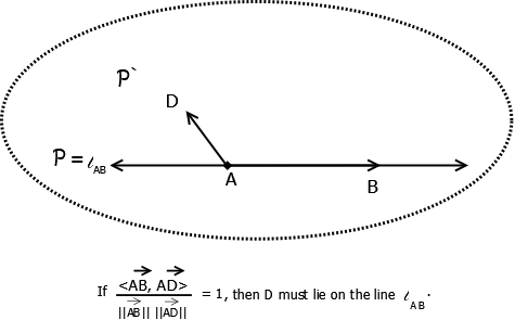
Figure 5.6. An illustration of Theorem 32.

Theorem 32.

Let $A,\;B$, and $D$ be three distinct points of $\mathcal{P}$ such that $\frac{\left<\overrightarrow{AB},\overrightarrow{AD}\right>_{A}}{||\overrightarrow{AB}||_{A}\;||\overrightarrow{AD}||_{A}}=-1$. Then the following is true:

• $$\frac{\left<\overrightarrow{AB},\overrightarrow{BD}\right>}{||\overrightarrow{AB}||_{A}\;||\overrightarrow{BD}||_{A}}=\pm 1;$$

• $$||\overrightarrow{AD}||_{A}=-||\overrightarrow{AB}||_{A}+||\overrightarrow{BD}||_{A};$$

  

  Figure 5.7. A depiction of three points $A,\;B,\;D$ when $||\overrightarrow{AD}||_{A}=-||\overrightarrow{AB}||_{A}+||\overrightarrow{BD}||_{A}$.

• there exists $t_{D}\in\mathbb{R}$ with $t_{D}<0$ such that $\overrightarrow{AD}=_{A}(t_{D})\overrightarrow{AB}$; thus the point $D$ lies on the line $l_{AB}$; see Figure 5.6.

Proof.

The proof of Part 1 is the same as the proof of Part 1 of Theorem 31 and is left to the reader. The proof of Part 2 is slightly more subtle. Since $\left<\overrightarrow{AB},\overrightarrow{AD}\right>_{A}=-||\overrightarrow{AB}||_{A}||\overrightarrow{AD}||_{A}$, Equation (5.14) becomes

(5.19) $$(||\overrightarrow{AD}||_{A}-||\overrightarrow{DB}||_{A})(||\overrightarrow{AD}||_{A}+||\overrightarrow{DB}||_{A})=-||\overrightarrow{AB}||_{A}\;(||\overrightarrow{AD}||_{A}\mp||\overrightarrow{DB}||_{A}).$$

A priori, it seems like Equation (5.19) has two possibilities. However, if we choose the minus sign option, Equation (5.19) becomes

$$(||\overrightarrow{AD}||_{A}-||\overrightarrow{DB}||_{A})(||\overrightarrow{AD}||_{A}+||\overrightarrow{DB}||_{A})=-||\overrightarrow{AB}||_{A}\;(||\overrightarrow{AD}||_{A}-||\overrightarrow{DB}||_{A})$$

which leads to the contradiction of $-||\overrightarrow{AB}||=||\overrightarrow{AD}||_{A}+||\overrightarrow{DB}||_{A}$. Thus Equation (5.19) really is

$$(||\overrightarrow{AD}||_{A}-||\overrightarrow{DB}||_{A})(||\overrightarrow{AD}||_{A}+||\overrightarrow{DB}||_{A})=-||\overrightarrow{AB}||_{A}\;(||\overrightarrow{AD}||_{A}+||\overrightarrow{DB}||_{A}),$$

which is equivalent to

(5.20) $$||\overrightarrow{AD}||_{A}-||\overrightarrow{BD}||_{A}=-||\overrightarrow{AB}||_{A}.$$

For the proof of Part 3 we need to first rewrite Equation (5.20) as

(5.21) $$||\overrightarrow{AD}||_{A}+||\overrightarrow{AB}||_{A}=||\overrightarrow{BD}||_{A}.$$

Equation (5.21) shows that $||\overrightarrow{AB}||_{A}\leq||\overrightarrow{BD}||_{A}$, which in turn implies

(5.22) $$1\leq\frac{||\overrightarrow{BD}||_{A}}{||\overrightarrow{AB}||_{A}}.$$

Also, Equation (5.20) implies that $-||\overrightarrow{AD}||_{A}=||\overrightarrow{AB}||_{A}\left(1-\frac{||\overrightarrow{BD}||_{A}}{||\overrightarrow{AB}||_{A}}\right)$. If we put

$$t_{D}=1-\frac{||\overrightarrow{BD}||_{A}}{||\overrightarrow{AB}||_{A}},$$

then we can rewrite the preceding equation as $-||\overrightarrow{AD}||_{A}=(t_{D})||\overrightarrow{AB}||_{A}$. Equation (5.22) implies $t_{D}\leq 0$. However if $t_{D}=0$, we get a contradiction since by hypothesis $A$ is distinct from $D$. So in fact $t_{D}<0$. Then

$$\frac{\left<\overrightarrow{AD},(t_{D})\overrightarrow{AB}\right>}{||\overrightarrow{AD}||_{A}\;||(t_{D})\overrightarrow{AB}||_{A}}=\frac{t_{D}\;\left<\overrightarrow{AD},\overrightarrow{AB}\right>}{|t_{D}|\;||\overrightarrow{AD}||_{A}\;||\overrightarrow{AB}||_{A}}=-\frac{\left<\overrightarrow{AD},\overrightarrow{AB}\right>}{||\overrightarrow{AD}||_{A}\;||\overrightarrow{AB}||_{A}}=1,$$

where the last equality made use of the hypothesis of the theorem. Furthermore

(5.23) $$||\overrightarrow{AD}||_{A}=-(t_{D})||\overrightarrow{AB}||_{A}=|t_{D}|||\overrightarrow{AB}||_{A}=||(t_{D})\overrightarrow{AB}||_{A},$$

and the rest of the argument proceeds analogously to proof of Part 3 of Theorem 31. ∎

Finally we are in the position to prove the arrow space equivalent of Euler’s first axiom, namely that for any two distinct points there exists a unique line that contains the two points.

Theorem 33.

(Existence of a Unique Line) Given any two distinct points $A$ and $B$ of $\mathcal{P}$, there exists a unique line $l_{AB}$ containing $A$ and $B$.

Proof.

Let $A$ and $B$ be two distinct points of $\mathcal{P}$. It follows by Axiom 3 that the set $\{F\in\mathcal{P}|\;\overrightarrow{AF}=_{A}(t)\;\overrightarrow{AB},\;\text{where}\;t\in\mathbb{R}\}$ is non-empty. By Definition 28 this set forms a line containing $A$ and $B$. To show the uniqueness part of this theorem, let $l_{AB}=\{F\in\mathcal{P}|\;\overrightarrow{AF}=_{A}(t)\;\overrightarrow{AB},\;\text{where}\;t\in\mathbb{R}\}$ and $l_{ML}=\{K\in\mathcal{P}|\;\overrightarrow{MK}=_{A}(s)\;\overrightarrow{ML},\;\text{where}\;s\in\mathbb{R}\}$ be two lines each of which contains $A$ and $B$, where $M$ and $L$ are any two distinct points that lie on $l_{AB}$ other than $A$ and $B$. By Definition 28 there exists $t_{M},\;t_{L}\in\mathbb{R}$ such that

(5.24) $$\overrightarrow{AM}=_{A}(t_{M})\;\overrightarrow{AB}\,\,\text{and}\,\,\overrightarrow{AL}=_{A}(t_{L})\;\overrightarrow{AB}.$$

To show that $l_{AB}=l_{ML}$, let $D\in l_{ML}$. It follows by Definition 28 that there exists $s_{D}\in\mathbb{R}$ with

(5.25) $$\overrightarrow{MD}=_{A}(s_{D})\;\overrightarrow{ML}.$$

See Figure 5.8.

Figure 5.8. The relationship between points $M$, $A$, $L$, $B$, and $D$ on line $l_{AB}$

In order to show that $D\in l_{AB}$, we need to find some $t_{D}\in\mathbb{R}$ such that $\overrightarrow{AD}=_{A}(t_{D})\;\overrightarrow{AB}.$ Since $A,\;B,\;M$, and $L$ satisfy the hypotheses of Lemma 30 we have $\frac{\left<\overrightarrow{ML},\overrightarrow{AB}\right>_{A}}{||\overrightarrow{ML}||_{A}\;||\overrightarrow{AB}||_{A}}=\pm 1$ which is equivalent to

(5.26) $$\left<\overrightarrow{ML},\overrightarrow{AB}\right>_{A}=\pm||\overrightarrow{ML}||_{A}\;||\overrightarrow{AB}||_{A}.$$

Since $\overrightarrow{AD}=_{A}\overrightarrow{AM}+_{A}\overrightarrow{MD}$, it follows by Equation (2.5) and Definition 7 that

(5.27) $$\frac{\left<\overrightarrow{AD},\overrightarrow{AB}\right>_{A}}{||\overrightarrow{AD}||_{A}\;||\overrightarrow{AB}||_{A}}=\frac{\left<\overrightarrow{AM},\overrightarrow{AB}\right>_{A}+\left<\overrightarrow{MD},\overrightarrow{AB}\right>_{A}}{\sqrt{\left<\overrightarrow{AD},\overrightarrow{AD}\right>_{A}}\;||\overrightarrow{AB}||_{A}}.$$

The numerator of the right hand side in the Equation (5.27) can be rewritten, using Equations (5.24), (5.25), (5.26), Definition (7), and Equation (2.8) as follows

$$\left<\overrightarrow{AM},\overrightarrow{AB}\right>_{A}+\left<\overrightarrow{MD},\overrightarrow{AB}\right>_{A} =t_{M}\;||\overrightarrow{AB}||_{A}^{2}+s_{D}\;\left<\overrightarrow{ML},\overrightarrow{AB}\right>_{A}$$

(5.28) $$=t_{M}\;||\overrightarrow{AB}||_{A}^{2}\pm s_{D}\;||\overrightarrow{ML}||_{A}\;||\overrightarrow{AB}||_{A}.$$

Next we simplify the denominator of the right hand side of the Equation (5.27) through a series of similar calculations. Equations (2.5) and (2.2) imply that

$$\left<\overrightarrow{AD},\overrightarrow{AD}\right>=\left<\overrightarrow{AM},\overrightarrow{AM}\right>_{A}+2\left<\overrightarrow{MD},\overrightarrow{AM}\right>_{A}+\left<\overrightarrow{MD},\overrightarrow{MD}\right>_{A}.$$

Using Equations (5.24), (5.25), (5.26), Definition 7, and Equation (2.8), the preceding equation can be rearranged as follows

$$\left<\overrightarrow{AD},\overrightarrow{AD}\right> =t_{M}^{2}\;||\overrightarrow{AB}||_{A}^{2}+2t_{M}s_{D}\;\left<\overrightarrow{ML},\overrightarrow{AB}\right>_{A}+s_{D}^{2}\;||\overrightarrow{ML}||_{A}^{2}$$

$$=t_{M}^{2}\;||\overrightarrow{AB}||_{A}^{2}\pm 2t_{M}s_{D}\;||\overrightarrow{ML}||_{A}\;||\overrightarrow{AB}||_{A}+s_{D}^{2}\;||\overrightarrow{ML}||_{A}^{2}$$

(5.29) $$=(t_{M}\;||\overrightarrow{AB}||_{A}\pm s_{D}||\overrightarrow{ML}||_{A})^{2}.$$

This means that the denominator of the right hand side of the Equation (5.27) is

(5.30) $$\sqrt{\left<\overrightarrow{AD},\overrightarrow{AD}\right>_{A}}\;||\overrightarrow{AB}||_{A}=|t_{M}\;||\overrightarrow{AB}||_{A}^{2}\pm s_{D}||\overrightarrow{ML}||_{A}\;||\overrightarrow{AB}||_{A}|.$$

By Combining Equations (5.27), (5.28), and (5.30) we find that

$$\frac{\left<\overrightarrow{AD},\overrightarrow{AB}\right>_{A}}{||\overrightarrow{AD}||_{A}\;||\overrightarrow{AB}||_{A}}=\frac{t_{M}\;||\overrightarrow{AB}||_{A}^{2}\pm s_{D}\;||\overrightarrow{ML}||_{A}\;||\overrightarrow{AB}||_{A}}{|t_{M}\;||\overrightarrow{AB}||_{A}^{2}\pm s_{D}||\overrightarrow{ML}||_{A}\;||\overrightarrow{AB}||_{A}|}=\pm 1.$$

Now by means of Theorem 31 and 32, we conclude that $D$ is a point on $l_{AB}$. This means that $l_{AB}\subseteq l_{ML}$, and a similar argument shows that $l_{ML}\subseteq l_{AB}$ to conclude that $l_{AB}=l_{ML}$. ∎

5.2. Equivalence Relation on $\mathcal{P}_{l_{A}}$

Now that we have the definition of the unique $l$ determined by $\overrightarrow{AB}$, we can restrict the arrow pre-inner product of $\mathcal{P}_{A}$ to $\mathcal{P}_{l_{A}}$ and use this restricted arrow pre-inner product to define an equivalence relation on the arrows of $\mathcal{P}_{l_{A}}$ which geometrically captures when two arrows have equal length and same direction. Because the arrow pre-inner product on $\mathcal{P}_{l_{A}}$ is the restriction of the pre-inner product of $\mathcal{P}_{A}$ to those arrows of $\mathcal{P}_{l_{A}}$, we will also use $\left<-,-\right>_{A}$ to denoted the arrow pre-inner product of $\mathcal{P}_{l_{A}}$.

The aforementioned construction is an internal construction for an arrow pre-inner product on $\mathcal{P}_{l_{A}}$, reminiscent of describing the restricted the inner product structure of direct summand in a vector space. We could also describe an external construction for developing an arrow pre-inner product on $\mathcal{P}_{l_{A}}$ . Instead of using restricted arrow pre-inner product from $\mathcal{P}_{A}$, we focus on $\mathcal{P}_{l_{A}}$ as a separate arrow space and apply the constructions of Section 2 with a new arrow pre-inner product, which denote as $\left<-,-\right>_{A_{l}}$. This new arrow pre-inner product must obey Axioms 1 and 2 and thus gives rises to a new definition on $P_{l_{A}}$ of scalar multiplication, which is denoted as $(a)_{A_{l}}\overrightarrow{AB}$.

Either construction provides the arrow space $\mathcal{P}_{l_{A}}$ with an arrow pre-inner product structure which is compatible with the propositions and theorems of this and the next subsection. It is a matter of taste as to which construction is preferred by the reader. For simplicity, we will write our results using the notation of the internal/restricted construction, but the reader should note that substitution of $\left<-,-\right>_{A}$ with $\left<-,-\right>_{A_{l}}$ and $(a)\overrightarrow{AB}$ with $(a)_{A_{l}}\overrightarrow{AB}$ will not change the validity of the results.

The algebraic definition of an equivalence relation on an arrow space $\mathcal{P}_{l_{A}}$ is provided below and will be essential to proving the existence of a unique parallel arrow; see Theorem 40.

Definition 34.

Given two distinct points $O$ and $P$, let $\mathcal{P}_{l_{A}}$ denote the arrow space determined by $l_{OP}$. Let $\overrightarrow{AB}$ and $\overrightarrow{CD}$ be two arrows in $\mathcal{P}_{l_{A}}$. We say that $\overrightarrow{AB}\;\Re_{l}\;\overrightarrow{CD}$, if and only if either $A=_{P}B$ and $C=_{P}D$, or

$$||\overrightarrow{AB}||_{A}=||\overrightarrow{CD}||_{A}\,\,\text{and}\,\,\left<\frac{\overrightarrow{AB}}{||\overrightarrow{AB}||_{A}},\;\frac{\overrightarrow{CD}}{||\overrightarrow{CD}||_{A}}\right>_{A}=1.$$

The following proposition and corollary are immediate consequences of Definition 34. They will play a role in the proof of Theorem 37.

Proposition 35.

If $\overrightarrow{AB}\;\Re_{l}\;\overrightarrow{CD}$ with $A=_{P}B$, then $C=_{P}D$.

Corollary 36.

If $\overrightarrow{AB}\;\Re_{l}\;\overrightarrow{CD}$ with $A\neq_{P}B$, then $C\neq_{P}D$.

Our next goal is to show that $\Re_{l}$ is an equivalence relation. To do so we need to introduce the following two theorems.

Theorem 37.

Let $l_{OP}$ be a line and $\mathcal{P}_{l}$ be the set of points on this line. Let $\overrightarrow{AB},\;\overrightarrow{CD},\;\overrightarrow{EF}$, and $\overrightarrow{GH}$ be in $\mathcal{P}_{l_{A}}$ such that $\overrightarrow{AB}\;\Re_{l}\;\overrightarrow{CD}$ and $\overrightarrow{EF}\;\Re_{l}\;\overrightarrow{GH}$. Then

(5.31) $$\left<\overrightarrow{AB},\overrightarrow{EF}\right>_{A}=\left<\overrightarrow{CD},\overrightarrow{GH}\right>_{A}.$$

Figure 5.9. An illustration of Theorem 37. Note that the equivalence between arrows is color coded where equivalent arrows share the same color.

Proof.

The proof of this theorem will be divided into two cases. First, if $A=_{P}B$ (similarly if $C=_{P}D$), then since $\overrightarrow{AB}\;\Re_{l}\;\overrightarrow{CD}$, Proposition 35 implies that $C=_{P}D$. Hence, Proposition 6 implies that

$$\left<\overrightarrow{AB},\overrightarrow{EF}\right>_{A}=\left<\overrightarrow{AA},\overrightarrow{EF}\right>_{A}=0\,\,\text{and}\,\,\left<\overrightarrow{CD},\overrightarrow{GH}\right>_{A}=\left<\overrightarrow{CC},\overrightarrow{GH}\right>_{A}=0.$$

Therefore, $\left<\overrightarrow{AB},\overrightarrow{EF}\right>_{A}=\left<\overrightarrow{CD},\overrightarrow{GH}\right>_{A}=0$. A similar argument follows if $E=_{P}F$ (or $G=_{P}H$).

Secondly, we consider the case where $A\neq_{P}B,\;C\neq_{P}D,\;E\neq_{P}F$, and $G\neq_{P}H$. Then none of the quantities $||\overrightarrow{AB}||_{A},\;||\overrightarrow{CD}||_{A},\;||\overrightarrow{EF}||_{A}$, and $||\overrightarrow{GH}||_{A}$ is zero. Our proof technique is to write all of the quantities that appear in Definition 34 in terms of $\overrightarrow{OP}$. Since $\overrightarrow{AB}=_{A}\overrightarrow{AO}+_{A}\overrightarrow{OB}$, Definition 7 and Equation (2.5) imply that

(5.32) $$||\overrightarrow{AB}||_{A}^{2}=||\overrightarrow{AO}+_{A}\overrightarrow{OB}||_{A}^{2}=\left<\overrightarrow{AO},\overrightarrow{AO}\right>_{A}+2\left<\overrightarrow{AO},\overrightarrow{OB}\right>_{A}+\left<\overrightarrow{OB},\overrightarrow{OB}\right>_{A}.$$

Since $A$ and $B$ are points in $\mathcal{P}_{l}$, by Definition 28 there exist $a,\;b\in\mathbb{R}$ such that

(5.33) $$\overrightarrow{OA}=_{A}(a)\;\overrightarrow{OP},\qquad\overrightarrow{OB}=_{A}(b)\;\overrightarrow{OP}.$$

It follows by Definition 4 that

(5.34) $$\overrightarrow{AO}=_{A}-((a)\;\overrightarrow{OP}).$$

Now if we substitute Equation (5.34) and the second equation from (5.33) into the right hand side of the Equation (5.32) and use Equations (2.8) and (2.6), we get

$$||\overrightarrow{AB}||_{A}^{2}=(a^{2}-2ab+b^{2})\;\left<\overrightarrow{OP},\overrightarrow{OP}\right>_{A}=(a-b)^{2}\;||\overrightarrow{OP}||_{A}^{2}.$$

Taking the positive square root of both sides in the above yields

(5.35) $$||\overrightarrow{AB}||_{A}=|a-b|\;||\overrightarrow{OP}||.$$

Similarly, we can write

$$\overrightarrow{CD}=_{A}\overrightarrow{CO}+_{A}\overrightarrow{OD},\,\,\,\overrightarrow{EF}=_{A}\overrightarrow{EO}+_{A}\overrightarrow{OF},\,\,\text{and}\,\,\,\overrightarrow{GH}=_{A}\overrightarrow{GO}+_{A}\overrightarrow{OH}.$$

Since $\overrightarrow{CD}$, $\overrightarrow{EF}$, and $\overrightarrow{GH}$ are in $\mathcal{P}_{l_{A}}$ we see that the points $C,\;D,E,\;F,\;G$, and $H$ lie on the line $l_{OP}$. Hence by Definition 28 there are real numbers $c,\;d,\;e,\;f,\;g$, and $h$ such that

(5.36) $$\overrightarrow{OC}=_{A}(c)\;\overrightarrow{OP},\,\,\;\overrightarrow{OD}=_{A} (d)\;\overrightarrow{OP},\,\,\,\overrightarrow{OE}=_{A}(e)\overrightarrow{OP},$$

(5.37) $$\overrightarrow{OF}=_{A}(f)\overrightarrow{OP},\,\,\;\overrightarrow{OG}=_{A} (g)\overrightarrow{OP},\,\,\,\overrightarrow{OH}=_{A}(h)\overrightarrow{OH}.$$

If we repeat the steps that led to Equations (5.32) through (5.35) we obtain

(5.38) $$||\overrightarrow{CD}||_{A}=|c-d|\;||\overrightarrow{OP}||,\;||\overrightarrow{EF}||_{A}=|e-f|\;||\overrightarrow{OP}||,\;||\overrightarrow{GH}||_{A}=|g-h|\;||\overrightarrow{OP}||.$$

Calculations similar to those used to derive Equation (5.35) show that

(5.39) $$\left<\overrightarrow{AB},\overrightarrow{EF}\right>_{A}=(a-b)(e-f)\left<\overrightarrow{OP},\overrightarrow{OP}\right>_{A},\,\,\left<\overrightarrow{CD},\overrightarrow{GH}\right>_{A}=(c-d)(g-h)\left<\overrightarrow{OP},\overrightarrow{OP}\right>_{A}.$$

We want to emphasize that none of the quantities $|a-b|,\;|c-d|,\;|e-f|$, and $|g-h|$ is zero. This is because, for example, $|a-b|=0$ means $a=b$. But by the two equations in (5.33) $a=b$ would imply that $\overrightarrow{OA}=_{A}\overrightarrow{OB}$. If this is true, then we would have, by Definition 3, that $A=_{P}B$. This is a contradiction to our the assumption of $A\neq_{P}B$. The same argument applies for $|c-d|,\;|e-f|$, and $|g-h|$.

Now by Equations (5.35), (5.38), and (5.39), we have

(5.40) $$\frac{\left<\overrightarrow{AB},\overrightarrow{EF}\right>_{A}}{||\overrightarrow{AB}||_{A}\;||\overrightarrow{EF}||_{A}}=\frac{(a-b)(e-f)}{|a-b|\;|e-f|},$$

and

(5.41) $$\frac{\left<\overrightarrow{CD},\overrightarrow{GH}\right>_{A}}{||\overrightarrow{CD}||_{A}\;||\overrightarrow{GH}||_{A}}=\frac{(c-d)(g-h)}{|c-d|\;|g-h|}.$$

In a similar manner we obtain

(5.42) $$\frac{\left<\overrightarrow{AB},\overrightarrow{CD}\right>_{A}}{||\overrightarrow{AB}||_{A}\;||\overrightarrow{CD}||_{A}}=\frac{(a-b)(c-d)}{|a-b|\;|c-d|},$$

and

(5.43) $$\frac{\left<\overrightarrow{EF},\overrightarrow{GH}\right>_{A}}{||\overrightarrow{EF}||_{A}\;||\overrightarrow{GH}||_{A}}=\frac{(e-f)(g-h)}{|e-f|\;|g-h|}.$$

Since $\overrightarrow{AB}\;\Re_{l}\;\overrightarrow{CD}$, Definition 34 implies that $\frac{\left<\overrightarrow{AB},\overrightarrow{CD}\right>_{A}}{||\overrightarrow{AB}||_{A}\;||\overrightarrow{CD}||_{A}}=1$. Hence, we conclude from Equation (5.42) that $\frac{(a-b)(c-d)}{|a-b|\;|c-d|}=1$, which means that

(5.44) $$(a-b)(c-d)>0.$$

A similar argument shows that

(5.45) $$(e-f)(g-h)>0.$$

The signs of the products $(a-b)(e-f)$ and $(c-d)(g-h)$ in Equations (5.40) and (5.41) will decide whether the right hand side of each of these two equations is $1$ or $-1$. We want to prove that the products $(a-b)(e-f)$ and $(c-d)(g-h)$ have the same sign. To do so, we set up the following table.

$a-b$	$+$	$+$	$-$	$-$
$c-d$	$+$	$+$	$-$	$-$
$e-f$	$+$	$-$	$+$	$-$
$g-h$	$+$	$-$	$+$	$-$
($a-b$)($e-f$)	$+$	$-$	$-$	$+$
($c-d$)($g-h$)	$+$	$-$	$-$	$+$

We conclude from the preceding table that the two products $(a-b)(e-f)$ and $(c-d)(g-h)$ are either both positive or negative. This means that in Equations (5.40) and (5.41) we have

(5.46) $$\frac{\left<\overrightarrow{AB},\overrightarrow{EF}\right>_{A}}{||\overrightarrow{AB}||_{A}\;||\overrightarrow{EF}||_{A}}=\frac{\left<\overrightarrow{CD},\overrightarrow{GH}\right>_{A}}{||\overrightarrow{CD}||_{A}\;||\overrightarrow{GH}||_{A}}=\pm 1.$$

Now since $\overrightarrow{AB}\;\Re_{l}\;\overrightarrow{CD}$ and $\overrightarrow{EF}\;\Re_{l}\;\overrightarrow{GH}$, we have that $||\overrightarrow{AB}||_{A}=||\overrightarrow{CD}||_{A}$ and $||\overrightarrow{EF}||_{A}=||\overrightarrow{GH}||_{A}$. Thus Equation (5.46) simplifies to the desired conclusion. ∎

With aid of Theorem 37 we prove the following result which will be used directly in proving that $\Re_{l}$ is an equivalence relation.

Theorem 38.

Let $l_{OP}$ be a line and $\mathcal{P}_{l}$ be the set of points on this line. Let $\overrightarrow{AB},\;\overrightarrow{CD},\;\overrightarrow{EF}$ be three arrows in $\mathcal{P}_{l_{A}}$ such that $\overrightarrow{AB}\;\Re_{l}\;\overrightarrow{CD}$ and $\overrightarrow{EF}\;\Re_{l}\;\overrightarrow{CD}$. Then $\overrightarrow{AB}\;\Re_{l}\;\overrightarrow{EF}$.

Proof.

First, if $A=_{P}B$ (similarly, if $C=_{P}D$ or $E=_{P}F$), then since $\overrightarrow{AB}\;\Re_{l}\;\overrightarrow{CD}$, it follows by Proposition 35 that $C=_{P}D$. Similarly, $C=_{P}D$ and $\overrightarrow{EF}\;\Re_{l}\;\overrightarrow{CD}$ means that $E=_{P}F$. We conclude that if $A=_{P}B$, then $E=_{P}F$, which means by Definition 34 that $\overrightarrow{AB}\;\Re_{l}\;\overrightarrow{EF}$.

Suppose now that $A\neq_{P}B,\;C\neq_{P}D$, and $E\neq_{P}F$. It follows by Lemma 8 that

(5.47) $$||\overrightarrow{AB}||_{A}\neq 0,\,\,\;||\overrightarrow{CD}||_{A}\neq 0,\,\,\;\text{and}\,\,\;||\overrightarrow{EF}||_{A}\neq 0.$$

Since $\overrightarrow{AB}\;\Re_{l}\;\overrightarrow{CD}$ and $\overrightarrow{EF}\;\Re_{l}\;\overrightarrow{CD}$, Definition 34 implies that

(5.48) $$\left<\frac{\overrightarrow{AB}}{||\overrightarrow{AB}||_{A}},\;\frac{\overrightarrow{CD}}{||\overrightarrow{CD}||_{A}}\right>_{A}=\left<\frac{\overrightarrow{EF}}{||\overrightarrow{EF}||_{A}},\;\frac{\overrightarrow{CD}}{||\overrightarrow{CD}||_{A}}\right>_{A}=1,$$

and

(5.49) $$||\overrightarrow{AB}||_{A}=||\overrightarrow{CD}||_{A},\qquad\;||\overrightarrow{CD}||_{A}=||\overrightarrow{EF}||_{A}.$$

Furthermore, since $\overrightarrow{AB}\;\Re_{l}\;\overrightarrow{CD}$ and $\overrightarrow{EF}\;\Re_{l}\;\overrightarrow{CD}$, it follows by Theorem 37 that

(5.50) $$\left<\overrightarrow{AB},\overrightarrow{EF}\right>_{A}=\left<\overrightarrow{CD},\overrightarrow{CD}\right>_{A}=||\overrightarrow{CD}||_{A}^{2}\neq 0.$$

Dividing both sides in Equation (5.50) by $||\overrightarrow{CD}||_{A}^{2}$ yields $\frac{\left<\overrightarrow{AB},\overrightarrow{EF}\right>_{A}}{||\overrightarrow{CD}||_{A}^{2}}=1$. This is equivalent to $\frac{\left<\overrightarrow{AB},\overrightarrow{EF}\right>_{A}}{||\overrightarrow{AB}||_{A}\;||\overrightarrow{EF}||_{A}}=1$, as $||\overrightarrow{AB}||_{A}=||\overrightarrow{CD}||_{A}=||\overrightarrow{EF}||_{A}$ by (5.49), which means by Definition 34 that $\overrightarrow{AB}\;\Re_{l}\;\overrightarrow{EF}$. ∎

Now we show that $\Re_{l}$ is an equivalence relation.

Theorem 39.

The relation $\Re_{l}$ in Definition 34 is an equivalence relation on $\mathcal{P}_{l_{A}}$.

Proof.

We first show that the relation $\Re_{l}$ is reflexive, that is $\overrightarrow{AB}\;\Re_{l}\;\overrightarrow{AB}$. Let $\overrightarrow{AB}\in\mathcal{P}_{l_{A}}$. If $A=_{P}B$, then it follows directly by Definition 7 that $\overrightarrow{AB}\;\Re_{l}\;\overrightarrow{AB}$. Now suppose that $A\neq_{P}B$. Then Definition 7 and Lemma 12 imply that

$$\left<\frac{\overrightarrow{AB}}{||\overrightarrow{AB}||_{A}},\;\frac{\overrightarrow{AB}}{||\overrightarrow{AB}||_{A}}\right>_{A}=\left|\left|\frac{\overrightarrow{AB}}{||\overrightarrow{AB}||_{A}}\right|\right|_{A}^{2}=1.$$

Thus, $\overrightarrow{AB}\;\Re_{l}\;\overrightarrow{AB}$ for any $\overrightarrow{AB}$ in $\mathcal{P}_{l_{A}}$. Next we show that $\Re_{l}$ is symmetric. Let $\overrightarrow{AB}\;\Re_{l}\;\overrightarrow{CD}$. If $A=_{P}B$ (similarly, if $C=_{P}D$), then since $\overrightarrow{AB}\;\Re_{l}\;\overrightarrow{CD}$, it follows by Proposition 35 that $C=_{P}D$. Now since $C=_{P}D$ and $A=_{P}B$, it follows by Definition 34 that $\overrightarrow{CD}\;\Re_{l}\;\overrightarrow{AB}$. If $A\neq_{P}B,\;C\neq_{P}D$, and $\overrightarrow{AB}\;\Re_{l}\;\overrightarrow{CD}$, then by Definition 34 we have

(5.51) $$||\overrightarrow{AB}||_{A}=||\overrightarrow{CD}||_{A}\,\,\text{and}\,\,\left<\frac{\overrightarrow{AB}}{||\overrightarrow{AB}||_{A}},\;\frac{\overrightarrow{CD}}{||\overrightarrow{CD}||_{A}}\right>_{A}=1$$

But by Equation (2.2) we have

(5.52) $$\left<\frac{\overrightarrow{AB}}{||\overrightarrow{AB}||_{A}},\;\frac{\overrightarrow{CD}}{||\overrightarrow{CD}||_{A}}\right>_{A}=\left<\frac{\overrightarrow{CD}}{||\overrightarrow{CD}||_{A}},\;\frac{\overrightarrow{AB}}{||\overrightarrow{AB}||_{A}}\right>_{A}=1.$$

It follows by the Equations (5.51), (5.52), and Definition 34 that $\overrightarrow{CD}\;\Re_{l}\;\overrightarrow{AB}$ which means that $\Re_{l}$ is symmetric. Now let $\overrightarrow{AB},\;\overrightarrow{CD},\;\overrightarrow{EF}$ be three arrows in $\mathcal{P}_{l_{A}}$ such that $\overrightarrow{AB}\;\Re_{l}\;\overrightarrow{CD}$ and $\overrightarrow{CD}\;\Re_{l}\;\overrightarrow{EF}$. The transitivity of $\Re_{l}$, that is $\overrightarrow{AB}\;\Re_{l}\;\overrightarrow{EF}$, follows immediately from the reflexivity of $\Re_{l}$ and Theorem 38. Therefore, $\Re_{l}$ is an equivalence relation on $\mathcal{P}_{l_{A}}$. ∎

5.3. Existence of Parallel Arrow in $\mathcal{P}_{l_{A}}$

Now we introduce the following important theorem which is the analog of the parallel axiom in Euclidean geometry. Furthermore, as we will later discover, this theorem supplants Axiom 5 in Sections 6 and 7, which shows that fewer axioms are needed to construct an arrow space whose underlying set of points is $\mathcal{P}_{l}$.

Theorem 40.

(Existence of a Unique Parallel Arrow) Given an arrow $\overrightarrow{AB}$ on a line $l_{AB}$ with $A\neq_{P}B$ and any point $P$ on $l_{AB}$, there exists a unique point $K$ on $l_{AB}$ (and a unique point $K^{\prime}$ on $l_{AB}$ ) such that $\overrightarrow{AB}\;\Re_{l}\;\overrightarrow{PK}$ (likewise $\overrightarrow{AB}\;\Re_{l}\;\overrightarrow{K^{\prime}P}$). See Figure 5.10.

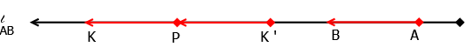
Figure 5.10. Existence of a parallel arrow.

Proof.

Let $\overrightarrow{AB}$ be an arrow of $\mathcal{P}_{l_{A}}$ with $A\neq_{P}B$. Let $P\in l_{AB}$ be any point. By Definition 28 and Theorem 13 there exists a unique $t\in\mathbb{R}$ such that

(5.53) $$\overrightarrow{AP}=_{A}(t)\overrightarrow{AB}.$$

By using Definition 4 this can be rewritten as

(5.54) $$\overrightarrow{PA}=_{A}-((t)\overrightarrow{AB}).$$

We are looking for some real number $s\in\mathbb{R}$ and a point $K\in l_{AB}$ such that

(5.55) $$\overrightarrow{AK}=_{A}(s)\overrightarrow{AB},$$

(5.56) $$||\overrightarrow{AB}||_{A}=||\overrightarrow{PK}||_{A},$$

and

(5.57) $$\left<\frac{\overrightarrow{AB}}{||\overrightarrow{AB}||_{A}},\;\frac{\overrightarrow{PK}}{||\overrightarrow{PK}||_{A}}\right>_{A}=1.$$

For the fixed points $A,\;B,\;P$, Equation (5.56) indicates that we should start with $||\overrightarrow{AB}||_{A}=||\overrightarrow{PK}||_{A}$ and uniquely solve for $K$ in a manner that satisfies Equations (5.55), (5.56), and (5.57). This will involve writing all the quantities in Equation (5.56) in terms of $\overrightarrow{AB}$. Since $\overrightarrow{PK}=\overrightarrow{PA}+\overrightarrow{AK}$, we have

$$||\overrightarrow{AB}||_{A}^{2} =||\overrightarrow{PK}||_{A}^{2}=||\overrightarrow{PA}+_{A}\overrightarrow{AK}||_{A}^{2}$$

(5.58) $$=\left<\overrightarrow{PA},\overrightarrow{PA}\right>_{A}+2\left<\overrightarrow{PA},\overrightarrow{AK}\right>_{A}+\left<\overrightarrow{AK},\overrightarrow{AK}\right>_{A}=(t-s)^{2}||\overrightarrow{AB}||_{A}^{2}.$$

Since $A\neq_{P}B$, Theorem 8 implies that $||\overrightarrow{AB}||_{A}\neq 0$. Hence we can divide both sides in Equation (5.58) by $||\overrightarrow{AB}||_{A}^{2}$ to get $(t-s)^{2}=1$. Taking the square root of both sides of the later equation yields

(5.59) $$t-s=\pm 1.$$

The above equation gives us two values of $s$, namely

(5.60) $$s_{0}=t+1\qquad s_{1}=t-1.$$

Notice that the number $t$ is fixed by the Equation (5.53) which yields the uniqueness of $s_{0},\;s_{1}$ in (5.60). The uniqueness of $s_{0}$ and $s_{1}$, in conjunction with Axiom 3, implies the uniqueness of $K$ and $K^{\prime}$, respectively. Therefore, we analyze the situation with $s_{0}$, (leaving $s_{1}$ to the reader, and express our claim as follows: there exists a unique point $K$ of $l_{AB}$ given by the equation

(5.61) $$\overrightarrow{AK}=_{A}(s_{0})\overrightarrow{AB},$$

where $s_{0}=t+1$. By construction this point satisfies Equation (5.56). It remains to confirm that this $K$ also satisfies Equation (5.57). Indeed, since $||\overrightarrow{PK}||_{A}=||\overrightarrow{AB}||_{A}$, we have

(5.62) $$\left<\frac{\overrightarrow{AB}}{||\overrightarrow{AB}||_{A}},\;\frac{\overrightarrow{PK}}{||\overrightarrow{PK}||_{A}}\right>_{A}=\left<\frac{\overrightarrow{AB}}{||\overrightarrow{AB}||_{A}},\;\frac{\overrightarrow{PK}}{||\overrightarrow{AB}||_{A}}\right>_{A}=\frac{\left<\overrightarrow{AB},\overrightarrow{PK}\right>_{A}}{\left<\overrightarrow{AB},\overrightarrow{AB}\right>_{A}}.$$

Hence, in order to prove the Equation (5.57), it is clear from the Equation (5.62) that we need only to show that

(5.63) $$\left<\overrightarrow{AB},\overrightarrow{PK}\right>_{A}=\left<\overrightarrow{AB},\overrightarrow{AB}\right>_{A}.$$

Now since $\overrightarrow{PK}=\overrightarrow{PA}+_{A}\overrightarrow{AK}$, by Equation (2.5) we have

$$\left<\overrightarrow{AB},\overrightarrow{PK}\right>_{A}=\left<\overrightarrow{AB},\overrightarrow{PA}+_{A}\overrightarrow{AK}\right>_{A}=\left<\overrightarrow{AB},\overrightarrow{PA}\right>_{A}+\left<\overrightarrow{AB},\overrightarrow{AK}\right>_{A}.$$

Since $\overrightarrow{AK}=_{A}(s_{0})\overrightarrow{AB}=_{A}(t+1)\;\overrightarrow{AB}$ and $\overrightarrow{PA}=_{A}-((t)\overrightarrow{AB)}$, the right hand side in the above becomes

$$\left<\overrightarrow{AB},\overrightarrow{PK}\right>_{A} =\left<\overrightarrow{AB},-((t)\overrightarrow{AB})\right>_{A}+\left<\overrightarrow{AB},(t+1)\;\overrightarrow{AB}\right>_{A}$$

$$=-t\left<\overrightarrow{AB},\overrightarrow{AB}\right>_{A}+(t+1)\left<\overrightarrow{AB},\overrightarrow{AB}\right>_{A}.$$

where the final equality follows from Equation (2.8). Rearranging the above yields $\left<\overrightarrow{AB},\overrightarrow{PK}\right>_{A}=\left<\overrightarrow{AB},\overrightarrow{AB}\right>_{A}$. This means that Equation (5.63) holds and combining Equations (5.62) and (5.63) yields Equation (5.57) as desired. ∎

6. An Equivalence Relation on Arrow Space

In this section we consider $\mathcal{P}$ to be any infinite set of points (including a set of points of a line). All definitions, axioms, and results from Sections 1 through 5 will be considered here unless otherwise is stated. For an arbitrary arrow space $\mathcal{P}_{A}$, we need to extend the definition of an equivalence relation on a line introduced in Section 5, which means restating Definition 34 in the context of an arbitrary arrow space and defining $\Re$. However, we need to make some changes to show that $\Re$ is an equivalence relation. In Section 5 we had all points contained in Line $l_{OP}$ and this restriction in direction allowed us to write all arrows as a scalar multiple of a fixed arrow $\overrightarrow{OP}$ and directly prove Theorem 37. This result was key to proving the transitivity of the relation $\Re_{l}$; see Theorem 38. However, if we try to prove the analog of Theorem 37 for a general arrow space we would face the difficulty expressing arrows in terms of one fixed arrow. Therefore, since this statement is crucial to prove transitivity of the relation $\Re$, we express it as an axiom, namely Axiom 4. Also, Theorem 40 from Section 5, namely the existence of a parallel arrow, must also be restated as Axiom 5 for the same reason. Once $\Re$ is shown to be an equivalence relation we can supplement $\mathcal{P}_{A}$ with vector algebra and form the associated vector space $\mathcal{P}_{v}$. The construction of $\mathcal{P}_{v}$ from $\mathcal{P}_{A}$ can also be applied to $\mathcal{P}_{l_{A}}$, taking into account that the statements of Axiom 4 and 5 from this section will be replaced by Theorems 37 and 40 respectively. Thus, less axioms are required in the case of line than the general case.

We start by defining a relation $\Re$ on $\mathcal{P}_{A}$.

Definition 41.

Let $\overrightarrow{AB}$ and $\overrightarrow{CD}$ be two arrows in $\mathcal{P}_{A}$. We say that $\overrightarrow{AB}\;\Re\;\overrightarrow{CD}$, if and only if either $A=_{P}B$ and $C=_{P}D$, or

$$||\overrightarrow{AB}||_{A}=||\overrightarrow{CD}||_{A}\,\,\text{and}\,\,\left<\frac{\overrightarrow{AB}}{||\overrightarrow{AB}||_{A}},\;\frac{\overrightarrow{CD}}{||\overrightarrow{CD}||_{A}}\right>_{A}=1.$$

We need the following axiom to prove transitivity of the relation $\Re$.

Axiom 4. Given $\overrightarrow{AB}$, $\overrightarrow{CD}$, $\overrightarrow{EF}$, and $\overrightarrow{GH}$ such that $\overrightarrow{AB}\;\Re\;\overrightarrow{CD}$ and $\overrightarrow{EF}\;\Re\;\overrightarrow{GH}$, then

(6.1) $$\left<\overrightarrow{AB},\overrightarrow{EF}\right>_{A}=\left<\overrightarrow{CD},\overrightarrow{GH}\right>_{A}.$$

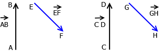
Figure 6.1. An illustration of Axiom 4 where equivalent arrows share the same color.

The proof of the following theorem is technically the same as that of Theorem 38, where Equation (6.1) of Axiom 4 is to be used instead of Theorem 37.

Theorem 42.

Let $\overrightarrow{AB},\;\overrightarrow{CD},\;\overrightarrow{EF}$ be three arrows in $\mathcal{P}_{A}$ such that $\overrightarrow{AB}\;\Re\;\overrightarrow{CD}$ and $\overrightarrow{CD}\;\Re\;\overrightarrow{EF}$. Then we have $\overrightarrow{AB}\;\Re\;\overrightarrow{EF}$.

Since proving that the relation $\Re$ is an equivalence relation is similar to the proof of Theorem 39 (notice that transitivity of $\Re$ follows directly from Theorem 42) we will state the theorem and skip the proof to avoid repetition.

Theorem 43.

The relation $\Re$ in Definition 41 is an equivalence relation on $\mathcal{P}_{A}$.

Now we are ready to introduce vectors.

Definition 44.

Consider the family of all equivalence classes that are obtained from Theorem 43 and denote it by $\mathcal{P}_{v}$. We call each equivalence class $[\overrightarrow{AB}]\in\mathcal{P}_{v}$ a vector, denoted by $v$. In particular, if $A=_{P}B$, then we call the equivalence class $[\overrightarrow{AA}]$ the zero vector and denote it by $\overrightarrow{0}$.

The following axiom represents a statement that combines equivalence classes (vectors), points, and arrows. Basically, it says that for any vector if a point is given, then there exist two unique arrows (one has the given point as a tail and the other has it as a head), and these two arrows are representatives of the given vector.

Axiom 5. (Existence of a Unique Parallel Arrow) Given an arrow $\overrightarrow{AB}$ with $A\neq_{P}B$ and any point $P\in\mathcal{P}$, there exists a unique point $K$ (and a unique point K’) in $\mathcal{P}$ such that $\overrightarrow{AB}\;\Re\;\overrightarrow{PK}$, that is

(6.2) $$||\overrightarrow{AB}||_{A}=||\overrightarrow{PK}||_{A}\;\;\,\text{and}\;\;\,\left<\frac{\overrightarrow{AB}}{||\overrightarrow{AB}||_{A}},\;\frac{\overrightarrow{PK}}{||\overrightarrow{PK}||_{A}}\right>_{A}=1,$$

where $P,\;K$ are the tail and head of $\overrightarrow{PK}$, respectively, (likewise, $||\overrightarrow{AB}||_{A}=||\overrightarrow{K^{\prime}P}||_{A}$, $\left<\frac{\overrightarrow{AB}}{||\overrightarrow{AB}||_{A}},\;\frac{\overrightarrow{K^{\prime}P}}{||\overrightarrow{K^{\prime}P}||_{A}}\right>_{A}=1$, where $K^{\prime},\;P$ are the tail and head of $\overrightarrow{K^{\prime}P}$, respectively.)

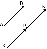
Figure 6.2. A depiction of Axiom 5 where $\overrightarrow{PK}$ and $\overrightarrow{K^{\prime}P}$ are equivalent to $\overrightarrow{AB}$.

Next we use Axiom 5 and Definition 5 to define an addition of the equivalence classes (vector addition). We use different notations for equality and addition of equivalence classes than that of arrows, namely $=_{V}$ and $+_{V}$, respectively.

Definition 45.

Let $[\overrightarrow{AB}]$ and $[\overrightarrow{CD}]\in\mathcal{P}_{v}$. Let $P$ be any point in $\mathcal{P}$. Consider the two unique arrows $\overrightarrow{KP}$ and $\overrightarrow{PL}$ that we get when we apply Axiom 5 to $\overrightarrow{AB}$ with the point $P$, and $\overrightarrow{CD}$ with the point $P$, respectively, such that $\overrightarrow{KP}\;\Re\;\overrightarrow{AB}$ and $\overrightarrow{PL}\;\Re\;\overrightarrow{CD}$. We define $[\overrightarrow{AB}]+_{V}[\overrightarrow{CD}]:=_{V}\;[\overrightarrow{KP}+_{A}\overrightarrow{PL}]=_{V}[\overrightarrow{KL}]$.

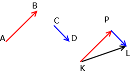
Figure 6.3. An illustration of vector addition where equivalent arrows share the same color.

Now we want to show that the addition $[\overrightarrow{AB}]+_{V}[\overrightarrow{CD}]$ given in Definition 45 is independent of the choice of the point $P$. This will be an easy task after we introduce the three following results.

Lemma 46.

Let $\overrightarrow{K_{1}P_{1}}$, $\overrightarrow{P_{1}L_{1}}$, $\overrightarrow{K_{2}P_{2}}$, and $\overrightarrow{P_{2}L_{2}}$ be such that (as in Figure (6.4)) $\overrightarrow{K_{1}P_{1}}\;\Re\;\overrightarrow{K_{2}P_{2}}$ and $\overrightarrow{P_{1}L_{1}}\;\Re\;\overrightarrow{P_{2}L_{2}}$, where $\{P_{1},\;K_{1},\;L_{1}\}$ and $\{P_{2},\;K_{2},\;L_{2}\}$ are disjoint sets. Then we have

(6.3) $$||\overrightarrow{K_{1}L_{1}}||_{A}=||\overrightarrow{K_{2}L_{2}}||_{A}.$$

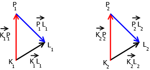
Figure 6.4. An illustration of Lemma 46. Note that the equivalence between arrows is color coded where equivalent arrows share the same color.

Proof.

Since $\overrightarrow{K_{1}P_{1}}\;\Re\;\overrightarrow{K_{2}P_{2}}$ and $\overrightarrow{P_{1}L_{1}}\;\Re\;\overrightarrow{P_{2}L_{2}}$, it follows by Definition 41 that

$$||\overrightarrow{K_{1}P_{1}}||_{A}=||\overrightarrow{K_{2}P_{2}}||_{A}\,\,\text{and}\,\,||\overrightarrow{P_{1}L_{1}}||_{A}=||\overrightarrow{P_{2}L_{2}}||_{A}.$$

Squaring both sides of each Equation in the above and using Definition 7 yields

(6.4) $$\left<\overrightarrow{K_{1}P_{1}},\overrightarrow{K_{1}P_{1}}\right>_{A}=\left<\overrightarrow{K_{2}P_{2}},\overrightarrow{K_{2}P_{2}}\right>_{A}\,\text{and}\,\left<\overrightarrow{P_{1}L_{1}},\overrightarrow{P_{1}L_{1}}\right>_{A}=\left<\overrightarrow{P_{2}L_{2}},\overrightarrow{P_{2}L_{2}}\right>_{A}$$

Also, since $\overrightarrow{K_{1}P_{1}}\;\Re\;\overrightarrow{K_{2}P_{2}}$ and $\overrightarrow{P_{1}L_{1}}\;\Re\;\overrightarrow{P_{2}L_{2}}$ we have, by Axiom 4 and Equation (2.2), that

(6.5) $$\left<\overrightarrow{K_{1}P_{1}},\overrightarrow{P_{1}L_{1}}\right>_{A}=\left<\overrightarrow{K_{2}P_{2}},\overrightarrow{P_{2}L_{2}}\right>_{A}=\left<\overrightarrow{P_{2}L_{2}},\overrightarrow{K_{2}P_{2}}\right>_{A}.$$

Now by Definitions 5 and 7 and Equations (6.4), (6.5), and (2.5) we have

$$||\overrightarrow{K_{2}L_{2}}||_{A}^{2} =\left<\overrightarrow{K_{2}P_{2}}+_{A}\overrightarrow{P_{2}L_{2}},\overrightarrow{K_{2}P_{2}}+_{A}\overrightarrow{P_{2}L_{2}}\right>_{A}$$

$$=\left<\overrightarrow{K_{2}P_{2}},\overrightarrow{K_{2}P_{2}}\right>_{A}+2\left<\overrightarrow{K_{2}P_{2}},\overrightarrow{P_{2}L_{2}}\right>_{A}+\left<\overrightarrow{P_{2}L_{2}},\overrightarrow{P_{2}L_{2}}\right>_{A}$$

$$=\left<\overrightarrow{K_{1}P_{1}},\overrightarrow{K_{1}P_{1}}\right>_{A}+2\left<\overrightarrow{K_{1}P_{1}},\overrightarrow{P_{1}L_{1}}\right>_{A}+\left<\overrightarrow{P_{1}L_{1}},\overrightarrow{P_{1}L_{1}}\right>_{A}$$

(6.6) $$=\left<\overrightarrow{K_{1}P_{1}}+_{A}\overrightarrow{P_{1}L_{1}},\overrightarrow{K_{1}P_{1}}+_{A}\overrightarrow{P_{1}L_{1}}\right>=||\overrightarrow{K_{1}L_{1}}||_{A}^{2}.$$

Taking the positive square root of both sides of Equation (6.6) gives the desired result. ∎

Theorem 47.

Let $\overrightarrow{K_{1}P_{1}}$, $\overrightarrow{P_{1}L_{1}}$, $\overrightarrow{P_{2}L_{2}}$, and $\overrightarrow{K_{2}P_{2}}$ be such that (see Figure (6.4)) $\overrightarrow{K_{1}P_{1}}\;\Re\;\overrightarrow{K_{2}P_{2}}$ and $\overrightarrow{P_{1}L_{1}}\;\Re\;\overrightarrow{P_{2}L_{2}}$, where $\{P_{1},\;K_{1},\;L_{1}\}$ and $\{P_{2},\;K_{2},\;L_{2}\}$ are disjoint sets. Then

(6.7) $$\frac{\left<\overrightarrow{K_{1}L_{1}},\overrightarrow{K_{2}L_{2}}\right>_{A}}{||\overrightarrow{K_{1}L_{1}}||_{A}||\overrightarrow{K_{2}L_{2}}||_{A}}=1.$$

Proof.

Since $\overrightarrow{K_{1}P_{1}}\;\Re\;\overrightarrow{K_{2}P_{2}}$, it follows by Definition 41 that

(6.8) $$\frac{\left<\overrightarrow{K_{1}P_{1}},\overrightarrow{K_{2}P_{2}}\right>_{A}}{||\overrightarrow{K_{1}P_{1}}||_{A}||\overrightarrow{K_{2}P_{2}}||_{A}}=1,\qquad||\overrightarrow{K_{1}P_{1}}||_{A}=||\overrightarrow{K_{2}P_{2}}||_{A}.$$

The two equations above together with Definition 7 imply that

(6.9) $$\left<\overrightarrow{K_{1}P_{1}},\overrightarrow{K_{2}P_{2}}\right>_{A}=||\overrightarrow{K_{1}P_{1}}||_{A}^{2}=\left<\overrightarrow{K_{1}P_{1}},\overrightarrow{K_{1}P_{1}}\right>_{A}.$$

Similarly, since $\overrightarrow{P_{1}L_{1}}\;\Re\;\overrightarrow{P_{2}L_{2}}$, we can get

(6.10) $$\left<\overrightarrow{P_{1}L_{1}},\overrightarrow{P_{2}L_{2}}\right>_{A}=\left<\overrightarrow{P_{1}L_{1}},\overrightarrow{P_{1}L_{1}}\right>_{A}.$$

Notice that Equation (6.7) is equivalent to

(6.11) $$\left<\overrightarrow{K_{1}L_{1}},\overrightarrow{K_{2}L_{2}}\right>_{A}=||\overrightarrow{K_{1}L_{1}}||_{A}||\overrightarrow{K_{2}L_{2}}||_{A}.$$

Also, we have by Lemma 46 that $||\overrightarrow{K_{1}L_{1}}||_{A}=||\overrightarrow{K_{2}L_{2}}||_{A}$. Hence, using this and Definition 7, Equation (6.11) becomes

(6.12) $$\left<\overrightarrow{K_{1}L_{1}},\overrightarrow{K_{2}L_{2}}\right>_{A}=||\overrightarrow{K_{1}L_{1}}||_{A}^{2}=\left<\overrightarrow{K_{1}L_{1}},\overrightarrow{K_{1}L_{1}}\right>_{A}.$$

Thus to prove this theorem it is enough to show that Equation (6.12) holds. Now by Definition 7 and Equation (2.5) we have

$$\left<\overrightarrow{K_{1}L_{1}},\overrightarrow{K_{2}L_{2}}\right>_{A} =\left<\overrightarrow{K_{1}P_{1}}+_{A}\overrightarrow{P_{1}L_{1}},\overrightarrow{K_{2}P_{2}}+_{A}\overrightarrow{P_{2}L_{2}}\right>_{A}$$

$$=\left<\overrightarrow{K_{1}P_{1}},\overrightarrow{K_{2}P_{2}}\right>_{A}+2\left<\overrightarrow{K_{1}P_{1}},\overrightarrow{P_{2}L_{2}}\right>_{A}+\left<\overrightarrow{P_{1}L_{1}},\overrightarrow{P_{2}L_{2}}\right>_{A}$$

(6.13) $$=\left<\overrightarrow{K_{1}P_{1}},\overrightarrow{K_{1}P_{1}}\right>_{A}+2\left<\overrightarrow{K_{1}P_{1}},\overrightarrow{P_{1}L_{1}}\right>_{A}+\left<\overrightarrow{P_{1}L_{1}},\overrightarrow{P_{1}L_{1}}\right>_{A},$$

where we used three applications of Axiom 4 to obtain the final equality. Applications of (2.5) and Definition 5, to the preceding equation yields

$$\left<\overrightarrow{K_{1}L_{1}},\overrightarrow{K_{2}L_{2}}\right>_{A}=\left<\overrightarrow{K_{1}L_{1}},\overrightarrow{K_{1}L_{1}}\right>_{A}.$$

This is exactly the Equation (6.12) which ends the proof of this theorem. ∎

Remark 48.

In the Equations (6.3) and (6.7) above, it is important to mention that the ruling of writing these equation is, for example, for the two arrows $\overrightarrow{K_{1}P_{1}}$, $\overrightarrow{P_{1}L_{1}}$, the corresponding arrow is to be written by taking the tail of the arrow whose head is the common point, and the head to be chosen as the head of the arrow whose tail is the common point. In this case the resultant arrow is $\overrightarrow{K_{1}L_{1}}$. Similarly, for $\overrightarrow{P_{2}L_{2}}$, and $\overrightarrow{K_{2}P_{2}}$, the resultant arrow is $\overrightarrow{K_{2}L_{2}}$.

Corollary 49.

Given $\overrightarrow{K_{1}P_{1}}$, $\overrightarrow{P_{1}L_{1}}$, $\overrightarrow{K_{2}P_{2}}$, and $\overrightarrow{P_{2}L_{2}}$ in an arrow space $\mathcal{P}_{A}$ where $\overrightarrow{K_{1}P_{1}}\;\Re\;\overrightarrow{K_{2}P_{2}},\;and\;\overrightarrow{P_{1}L_{1}}\;\Re\;\overrightarrow{P_{2}L_{2}}$, and where $\{P_{1},\;K_{1},\;L_{1}\}\cap\{P_{2},\;K_{2},\;L_{2}\}=\emptyset$, then $\overrightarrow{K_{1}L_{1}}\;\Re\;\overrightarrow{K_{2}L_{2}}$.

Proof.

By Lemma 46 we have

(6.14) $$||\overrightarrow{K_{1}L_{1}}||_{A}=||\overrightarrow{K_{2}L_{2}}||_{A}.$$

Also, by Theorem 47 we have

(6.15) $$\frac{\left<\overrightarrow{K_{1}L_{1}},\overrightarrow{K_{2}L_{2}}\right>_{A}}{||\overrightarrow{K_{1}L_{1}}||_{A}||\overrightarrow{K_{2}L_{2}}||_{A}}=1.$$

By means of Definition 41, Equations (6.14), (6.15) imply that $\overrightarrow{K_{1}L_{1}}\;\Re\;\overrightarrow{K_{2}L_{2}}$, as desired. ∎

Next we use Corollary 49 to prove that the addition of vectors in Definition 45 is independent from the choice of the point $P$.

Theorem 50.

Given any two equivalence classes $[\overrightarrow{AB}],\;[\overrightarrow{CD}]\in\mathcal{P}_{v}$, the addition, $[\overrightarrow{AB}]+_{V}[\overrightarrow{CD}]$ as given in Definition 45 is independent of the choice of the point $P$.

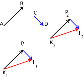
Figure 6.5. Independent Vector Addition. Note that the equivalence between arrows is color coded where equivalent arrows share the same color.

Proof.

Let $[\overrightarrow{AB}],\;[\overrightarrow{CD}]\in\mathcal{P}_{v}$ and let $P_{1},\;P_{2}$ be any two distinct points in $\mathcal{P}$. Using Axiom 5 let $\overrightarrow{K_{1}P_{1}}$ and $\overrightarrow{P_{1}L_{1}}$ be such that $\overrightarrow{K_{1}P_{1}}\;\Re\;\overrightarrow{AB}$ and $\overrightarrow{P_{1}L_{1}}\;\Re\;\overrightarrow{CD}$; and also let $\overrightarrow{K_{2}P_{2}}$ and $\overrightarrow{P_{2}L_{2}}$ be such that $\overrightarrow{K_{2}P_{2}}\;\Re\;\overrightarrow{AB}$ and $\overrightarrow{P_{2}L_{2}}\;\Re\;\overrightarrow{CD}$ (see Figure 6.5). Then since the relation $\Re$ is transitive, it follows that

(6.16) $$\overrightarrow{K_{1}P_{1}}\;\Re\;\overrightarrow{K_{2}P_{2}},\;\,\text{and}\;\,\overrightarrow{P_{1}L_{1}}\;\Re\;\overrightarrow{P_{2}L_{2}}.$$

To show that Definition 45 is independent of the choice of any point, it is enough to show that $\overrightarrow{K_{1}L_{1}}\;\Re\;\overrightarrow{K_{2}L_{2}}$. This is an immediate result of Remark 48 and Corollary 49. ∎

Now we define vector scalar multiplication

Definition 51.

Let $t\in\mathbb{R}$ and $u=[\overrightarrow{AB}]$ be any vector, where $\overrightarrow{AB}$ is some representative of an equivalence class. We define the scalar multiplication

$$t\;u=t\;[\overrightarrow{AB}]:=_{V}[(t)\;\overrightarrow{AB}].$$

In order to show that product $t\;u$ in Definition 51 is independent of the choice of the arrow $\overrightarrow{AB}$, we need the following lemma.

Lemma 52.

For any two arrows $\overrightarrow{AB},\;\overrightarrow{CD}$ and any $t\in\mathbb{R}$ if $\overrightarrow{AB}\;\Re\;\overrightarrow{CD}$, then $(t)\;\overrightarrow{AB}\;\Re\;(t)\;\overrightarrow{CD}$.

Proof.

If $A=_{P}B$, then since $\overrightarrow{AB}\;\Re\;\overrightarrow{CD}$, we would have by Proposition 35 that $C=_{P}D$. Then for any $t\in\mathbb{R}$ we have by Definition 9 that

$$(t)\;\overrightarrow{AB}=_{A}(t)\;\overrightarrow{AA}=_{A}\overrightarrow{AA},\;\,\text{and}\,\;(t)\;\overrightarrow{CD}=_{A}(t)\;\overrightarrow{CC}=_{A}\overrightarrow{CC}.$$

Thus, since we have by Definition 41 that $\overrightarrow{AA}\;\Re\;\overrightarrow{CC}$, we conclude that $(t)\;\overrightarrow{AB}\;\Re\;(t)\;\overrightarrow{CD}$. Now let $\overrightarrow{AB},\;\overrightarrow{CD}\in\mathcal{P}_{A}$, with $A\neq_{P}B,\;C\neq_{P}D$, such that $\overrightarrow{AB}\;\Re\;\overrightarrow{CD}$. If $t=0$, the if follows by Definition 9 that

$$(t)\;\overrightarrow{AB}=_{A}(0)\;\overrightarrow{AB}=_{A}\overrightarrow{AA},\;\,\text{and}\,\;(t)\;\overrightarrow{CD}=_{A}(0)\;\overrightarrow{CD}=_{A}\overrightarrow{CC}.$$

Thus, again we have by Definition 41 that $\overrightarrow{AA}\;\Re\;\overrightarrow{CC}$ and we conclude that $(t)\;\overrightarrow{AB}\;\Re\;(t)\;\overrightarrow{CD}$. We now consider that $\overrightarrow{AB},\;\overrightarrow{CD}\in\mathcal{P}_{A}$, with $A\neq_{P}B,\;C\neq_{P}D$, such that $\overrightarrow{AB}\;\Re\;\overrightarrow{CD}$ and $t\neq 0$. By Definition 41, we know that

(6.17) $$||\overrightarrow{AB}||_{A}=||\overrightarrow{CD}||_{A}\,\,\text{and}\,\,\left<\frac{\overrightarrow{AB}}{||\overrightarrow{AB}||_{A}},\;\frac{\overrightarrow{CD}}{||\overrightarrow{CD}||_{A}}\right>_{A}=1.$$

By Lemma 12 and (6.17) we have

(6.18) $$||(t)\;\overrightarrow{AB}||_{A}=|t|\;||\overrightarrow{AB}||_{A}=|t|\;||\overrightarrow{CD}||_{A}=||(t)\;\overrightarrow{CD}||_{A}.$$

Also, by Lemma 12, (2.8), and Equation (6.17) we have

(6.19) $$\left<\frac{(t)\;\overrightarrow{AB}}{||(t)\;\overrightarrow{AB}||_{A}},\;\frac{(t)\;\overrightarrow{CD}}{||(t)\;\overrightarrow{CD}||_{A}}\right>_{A}=\left<\frac{(t)\;\overrightarrow{AB}}{|t|\;||\overrightarrow{AB}||_{A}},\;\frac{(t)\;\overrightarrow{CD}}{|t|\;||\overrightarrow{CD}||_{A}}\right>_{A}=1.$$

Combining (6.18) and (6.19) with Definition 41 shows that

$$(t)\;\overrightarrow{AB}\;\Re\;(t)\;\overrightarrow{CD}.$$

∎

7. The Equivalence Classes Of arrows as a Vector space

In this section we show that the set $\mathcal{P}_{v}$ of all equivalence classes of arrows with the two operations, addition and scalar multiplication, from Definitions 45 and 51 satisfy all the axioms of vector space. Definitions 45 and 51 imply that $\mathcal{P}_{v}$ is closed under these two operations, namely that adding two equivalence classes and multiplying a scalar in any equivalence class is again an equivalence class. We now prove the remaining eight axioms of a vector space. We start by showing that the addition $+_{V}$ is commutative.

Theorem 53.

The addition $+_{V}$ is commutative, that is for any $[\overrightarrow{AB}]$ and $[\overrightarrow{CD}]$ in $\mathcal{P}_{v}$ we have

(7.1) $$[\overrightarrow{AB}]+_{V}[\overrightarrow{CD}]=_{V}[\overrightarrow{CD}]+_{V}[\overrightarrow{AB}].$$

Proof.

Let $P_{1}$ be any point and use Axiom 5 to find the arrows $\overrightarrow{K_{1}P_{1}}$ and $\overrightarrow{P_{1}L_{1}}$ such that (see Figure 7.1)

(7.2) $$\overrightarrow{K_{1}P_{1}}\;\Re\;\overrightarrow{AB}\qquad\text{and}\qquad\overrightarrow{P_{1}L_{1}}\;\Re\;\overrightarrow{CD}.$$

Then by Definition 45 we have

(7.3) $$[\overrightarrow{AB}]+_{V}[\overrightarrow{CD}]=[\overrightarrow{K_{1}P_{1}}+_{A}\overrightarrow{P_{1}L_{1}}]=[\overrightarrow{K_{1}L_{1}}].$$

On the other hand, let $P_{2}$ be any point and use Axiom 5 to find the arrows $\overrightarrow{K_{2}P_{2}}$ and $\overrightarrow{P_{2}L_{2}}$ such that (see Figure (7.1) below)

(7.4) $$\overrightarrow{P_{2}L_{2}}\;\Re\;\overrightarrow{AB}\qquad\text{and}\qquad\overrightarrow{K_{2}P_{2}}\;\Re\;\overrightarrow{CD}.$$

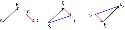
Figure 7.1. An illustration of Theorem 53. Note that the equivalence between arrows is color coded where equivalent arrows share the same color.

Then we have again by Definition 45 that

(7.5) $$[\overrightarrow{CD}]+_{V}[\overrightarrow{AB}]=[\overrightarrow{K_{2}P_{2}}+_{A}\overrightarrow{P_{2}L_{2}}]=[\overrightarrow{K_{2}L_{2}}].$$

Equations (7.3) and (7.5) imply that we need to prove

(7.6) $$\overrightarrow{K_{1}L_{1}}\;\Re\;\overrightarrow{K_{2}L_{2}}.$$

By Equations (7.2) and (7.4), and the transitivity of the relation $\Re$, we have

(7.7) $$\overrightarrow{K_{1}P_{1}}\;\Re\;\overrightarrow{P_{2}L_{2}}\qquad\text{and}\qquad\overrightarrow{P_{1}L_{1}}\;\Re\;\overrightarrow{K_{2}P_{2}}.$$

Applications of Remark 48 and Corollary 49 to Equation (7.7) yields the desired result of Equation (7.6). ∎

We show also that the addition $+_{V}$ is associative and identify the additive identity, namely $[\overrightarrow{PP}]$ where $P$ is any point in $\mathcal{P}$.

Theorem 54.

For any $[\overrightarrow{AB}],\;[\overrightarrow{CD}]$, and $[\overrightarrow{EF}]$ in $\mathcal{P}_{v}$ we have

• addition $+_{V}$ is associative, that is

  (7.8) $$([\overrightarrow{AB}]+_{V}[\overrightarrow{CD}])+_{V}[\overrightarrow{EF}]=_{V}[\overrightarrow{AB}]+_{V}([\overrightarrow{CD}]+_{V}[\overrightarrow{EF}]);$$

• for any point $P$ and any $[\overrightarrow{AB}]$, $[\overrightarrow{AB}]+_{V}[\overrightarrow{PP}]=_{V}[\overrightarrow{AB}].$

Proof.

(1) Let $P_{1}$ be any point in $\mathcal{P}$. Then by using Axiom 5, we let $\overrightarrow{K_{1}P_{1}}$ and $\overrightarrow{P_{1}L_{1}}$ be in $\mathcal{P}_{A}$ such that

$$\overrightarrow{K_{1}P_{1}}\;\Re\;\overrightarrow{AB}\qquad\text{and}\qquad\overrightarrow{P_{1}L_{1}}\;\Re\;\overrightarrow{CD}.$$

Also, by an application of Axiom 5 to the arrow $\overrightarrow{EF}$ and the point $L_{1}$, we get the arrow $\overrightarrow{L_{1}T_{1}}$ such that

$$\overrightarrow{L_{1}T_{1}}\;\Re\;\overrightarrow{EF}.$$

See Figure 7.2.

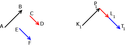
Figure 7.2. An illustration used in the proof of the associativity of vector addition. As usual, arrow equivalence is denoted via color coding.

Now by Definition 45 and Theorem 20 we have

$$([\overrightarrow{AB}]+_{V}[\overrightarrow{CD}])+_{V}[\overrightarrow{EF}] =_{V}[\overrightarrow{K_{1}P_{1}}+_{A}\overrightarrow{P_{1}L_{1}}]+_{V}[\overrightarrow{L_{1}T_{1}}]$$

$$=_{V}[(\overrightarrow{K_{1}P_{1}}+_{A}\overrightarrow{P_{1}L_{1}})+_{A}\overrightarrow{L_{1}T_{1}}]$$

$$=_{V}[\overrightarrow{K_{1}P_{1}}+_{A}(\overrightarrow{P_{1}L_{1}}+_{A}\overrightarrow{L_{1}T_{1}})]$$

$$=_{V}[\overrightarrow{K_{1}P_{1}}]+_{V}[\overrightarrow{P_{1}L_{1}}+_{A}\overrightarrow{L_{1}T_{1}}]$$

$$=_{V}[\overrightarrow{AB}]+_{V}([\overrightarrow{CD}]+_{V}[\overrightarrow{EF}]).$$

Thus, the addition $+_{V}$ is associative.

(2) Let $P$ be any point and $[\overrightarrow{AB}]$ be any given vector. Then by Axiom 5 there exists a unique arrow, say $\overrightarrow{KP}$, such that $\overrightarrow{KP}\;\Re\;\overrightarrow{AB}$. By Definition 45 we have

$$[\overrightarrow{AB}]+_{V}[\overrightarrow{PP}] =_{V}[\overrightarrow{KP}+_{A}\overrightarrow{PP}]=_{V}[\overrightarrow{KP}]=_{V}[\overrightarrow{AB}].$$

∎

Next we prove that for any $[\overrightarrow{AB}]$ in $\mathcal{P}_{v}$ there exists the additive inverse which is $[-\overrightarrow{AB}]$.

Theorem 55.

For any $[\overrightarrow{AB}]$ in $\mathcal{P}_{v}$ we have

$$[\overrightarrow{AB}]+_{V}[-\overrightarrow{AB}]=_{V}[\overrightarrow{AA}].$$

Proof.

By Definition 4 we have $-\overrightarrow{AB}=_{A}\overrightarrow{BA}$, and since the relation $\Re$ is reflexive we have $-\overrightarrow{AB}\;\Re\;\overrightarrow{BA}.$ It follows by Definitions 5 and 45 and that

$$[\overrightarrow{AB}]+_{V}[-\overrightarrow{AB}]=_{V}[\overrightarrow{AB}]+_{V}[\overrightarrow{BA}]=_{V}[\overrightarrow{AB}+_{A}\overrightarrow{BA}]=_{V}[\overrightarrow{AA}].$$

∎

In the following theorem we prove that the scalar multiplication is associative and distributive.

Theorem 56.

For any $[\overrightarrow{AB}]$ in $\mathcal{P}_{v}$ and $s,\;t\in\mathbb{R}$ we have

• $t\;s\;[\overrightarrow{AB}]=_{V}t\;[(s)\;\overrightarrow{AB}]$,

• for any arrow $\overrightarrow{AB}$ we have $(t+s)\;[\overrightarrow{AB}]=_{V}t\;[\overrightarrow{AB}]+_{V}s\;[\overrightarrow{AB}]$.

Proof.

(1) Let $t,\;s\in\mathbb{R}$ and $\overrightarrow{AB}$ be any arrow. By Definition 51 we have

(7.9) $$s\;[\overrightarrow{AB}]=_{V}[(s)\;\overrightarrow{AB}].$$

An application of Definition 51 to Equation (7.9) yields

$$t\;s\;[\overrightarrow{AB}]=_{V}t\;[(s)\;\overrightarrow{AB}].$$

(2) If $A=_{P}B$, the identity holds trivially. So without loss of generality assume $A\neq_{P}B$. Let $K$ and $L$ be some points that lie on the line $l_{AB}$ such that

(7.10) $$(t)\;\overrightarrow{AB}=_{A}\overrightarrow{AK}\qquad\text{and}\qquad(s)\;\overrightarrow{AB}=_{A}\overrightarrow{AL},$$

By Definition 51 and Equation (7.10) we have

(7.11) $$t\;[\overrightarrow{AB}]+_{V}s\;[\overrightarrow{AB}] =_{V}[(t)\;\overrightarrow{AB}]+_{V}[(s)\;\overrightarrow{AB}]=_{V}[\overrightarrow{AK}]+_{V}[\overrightarrow{AL}].$$

If we use Axiom 5 for the arrow $\overrightarrow{AL}$ and the point $K$, we get the arrow $\overrightarrow{KD}$ where $\overrightarrow{AL}\;\Re\;\overrightarrow{KD}$. Thus by Definition 45 we can rewrite Equation (7.11) as

(7.12) $$t\;[\overrightarrow{AB}]+_{V}s\;[\overrightarrow{AB}]=_{V}[\overrightarrow{AK}+_{A}\overrightarrow{KD}]=_{V}[\overrightarrow{AD}].$$

On the other hand, by Definition 51 we have

(7.13) $$(t+s)\;[\overrightarrow{AB}]=_{V}[(t+s)\;\overrightarrow{AB}].$$

Equations (7.12) and (7.13) imply that proving $(t+s)\;[\overrightarrow{AB}]=_{V}t\;[\overrightarrow{AB}]+_{V}s\;[\overrightarrow{AB}]$ is equivalent to proving

(7.14) $$\overrightarrow{AD}\;\Re\;(t+s)\;\overrightarrow{AB}.$$

Various applications of Definition 7 and Equation (2.5) show that

$$||\overrightarrow{AD}||_{A}^{2} =\left<\overrightarrow{AD},\overrightarrow{AD}\right>_{A}=\left<\overrightarrow{AK}+_{A}\overrightarrow{KD},\overrightarrow{AK}+_{A}\overrightarrow{KD}\right>_{A}$$

(7.15) $$=\left<\overrightarrow{AK},\overrightarrow{AK}\right>_{A}+2\left<\overrightarrow{AK},\overrightarrow{KD}\right>_{A}+\left<\overrightarrow{KD},\overrightarrow{KD}\right>_{A}.$$

Moreover, Equations (2.8) and (7.10) and Definition 7 imply that

(7.16) $$\left<\overrightarrow{AK},\overrightarrow{AK}\right>_{A}=\left<(t)\;\overrightarrow{AB},(t)\;\overrightarrow{AB}\right>_{A}=t^{2}\;\left<\overrightarrow{AB},\overrightarrow{AB}\right>_{A}=t^{2}\;||\overrightarrow{AB}||_{A}^{2}.$$

Equation (7.10) and the fact that $\overrightarrow{AL}\;\Re\;\overrightarrow{KD}$ shows that $\overrightarrow{KD}\;\Re\;(s)\;\overrightarrow{AB}$, and since the relation $\Re$ is reflexive we have $\overrightarrow{AK}\;\Re\;\overrightarrow{AK}$. Then an application of Axiom 4 implies that

(7.17) $$\left<\overrightarrow{AK},\overrightarrow{KD}\right>_{A}=\left<\overrightarrow{AK},(s)\;\overrightarrow{AB}\right>_{A}=\left<(t)\;\overrightarrow{AB},(s)\;\overrightarrow{AB}\right>_{A}=t\;s\;||\overrightarrow{AB}||_{A}^{2}.$$

Similarly, we find that

(7.18) $$\left<\overrightarrow{KD},\overrightarrow{KD}\right>_{A}=s^{2}\;||\overrightarrow{AB}||_{A}^{2}.$$

If we plug the Equations (7.16), (7.17), and (7.18) into Equation (7.15), we get

$$||\overrightarrow{AD}||_{A}^{2}=t^{2}\;||\overrightarrow{AB}||_{A}^{2}+2t\;s\;||\overrightarrow{AB}||_{A}^{2}+s^{2}\;||\overrightarrow{AB}||_{A}^{2}=(t+s)^{2}\;||\overrightarrow{AB}||_{A}^{2}.$$

Taking the positive square root of both sides in the above yields

(7.19) $$||\overrightarrow{AD}||_{A} =(t+s)\;||\overrightarrow{AB}||_{A}.$$

Furthermore Equation (2.8), Lemma 12, and Definition 5 imply that

$$\frac{\left<(t+s)\;\overrightarrow{AB},\overrightarrow{AD}\right>_{A}}{||(t+s)\;\overrightarrow{AB}||_{A}\;||\overrightarrow{AD}||_{A}}=\frac{(t+s)\;\left<\overrightarrow{AB},\overrightarrow{AD}\right>_{A}}{|t+s|\;||\overrightarrow{AB}||_{A}\;||\overrightarrow{AD}||_{A}}$$

(7.20) $$=\frac{(t+s)}{|t+s|}\frac{\left<\overrightarrow{AB},\overrightarrow{AK}+_{A}\overrightarrow{KD}\right>_{A}}{||\overrightarrow{AB}||_{A}\;||\overrightarrow{AD}||_{A}}=\frac{(t+s)}{|t+s|}\left(\frac{\left<\overrightarrow{AB},\overrightarrow{AK}\right>_{A}}{||\overrightarrow{AB}||_{A}\;||\overrightarrow{AD}||_{A}}+\frac{\left<\overrightarrow{AB},\overrightarrow{KD}\right>_{A}}{||\overrightarrow{AB}||_{A}\;||\overrightarrow{AD}||_{A}}\right).$$

By definition,

(7.21) $$\left<\overrightarrow{AB},\overrightarrow{AK}\right>_{A}=\left<\overrightarrow{AB},(t)\;\overrightarrow{AB}\right>_{A}=t\left<\overrightarrow{AB},\overrightarrow{AB}\right>_{A},$$

and by an application of Axiom 4

(7.22) $$\left<\overrightarrow{AB},\overrightarrow{KD}\right>_{A}=\left<\overrightarrow{AB},(s)\;\overrightarrow{AB}\right>_{A}=s\left<\overrightarrow{AB},\overrightarrow{AB}\right>_{A}.$$

If we plug Equations (7.19), (7.21), and (7.22) into Equation (7.20), we get

$$\frac{\left<(t+s)\;\overrightarrow{AB},\overrightarrow{AD}\right>_{A}}{||(t+s)\;\overrightarrow{AB}||_{A}\;||\overrightarrow{AD}||_{A}} =\frac{(t+s)}{|t+s|}\left(\frac{t\left<\overrightarrow{AB},\overrightarrow{AB}\right>_{A}}{||\overrightarrow{AB}||_{A}\;||\overrightarrow{AD}||_{A}}+\frac{s\left<\overrightarrow{AB},\overrightarrow{AB}\right>_{A}}{||\overrightarrow{AB}||_{A}\;||\overrightarrow{AD}||_{A}}\right)$$

(7.23) $$=\frac{(t+s)^{2}}{|t+s|^{2}}\frac{\left<\overrightarrow{AB},\overrightarrow{AB}\right>_{A}}{||\overrightarrow{AB}||_{A}^{2}}=1,$$

where the last equality follows from Definition 7. Now by means of Definition 41, Equations (7.19) and (7.23) imply that $\overrightarrow{AD}\;\Re\;(t+s)\;\overrightarrow{AB}$, that is Equation (7.14) holds.∎

Finally we show another distributive property of the scalar multiplication and identify the vector scalar multiplicative identity as the real number $1$.

Theorem 57.

For any $[\overrightarrow{AB}],\;[\overrightarrow{CD}]$ in $\mathcal{P}_{v}$ and any $t\in\mathbb{R}$ we have

• $t\;([\overrightarrow{AB}]+_{V}[\overrightarrow{CD}])=_{V}t\;[\overrightarrow{AB}]+_{V}t\;[\overrightarrow{CD}]$,

• $1\;[\overrightarrow{AB}]=_{V}[\overrightarrow{AB}]$.

Proof.

(1) If $A=_{P}B$ or $C=_{P}D$, the identity holds trivially. So assume $A\neq_{P}B$ and $C\neq_{P}D$. Using Axiom 5 for the arrow $\overrightarrow{CD}$ and the point $B$ we get the arrow $\overrightarrow{BK}$ such that $\overrightarrow{CD}\;\Re\;\overrightarrow{BK}$. Definitions 45 and 51 imply that

$$t\;([\overrightarrow{AB}]+_{V}[\overrightarrow{CD}])=_{V}t\;[\overrightarrow{AB}+_{A}\overrightarrow{BK}]=_{V}t\;[\overrightarrow{AK}]=[(t)\;\overrightarrow{AK}]=[\overrightarrow{AH}].$$

for some point $H$ that lies on the line $l_{AK}$ with $(t)\;\overrightarrow{AK}\;\Re\;\overrightarrow{AH}$. It follows from the preceding relation and Lemma 12 that $|t|\;||\overrightarrow{AK}||_{A}=_{A}||\overrightarrow{AH}||_{A}$. Now let

(7.24) $$(t)\;\overrightarrow{AB}=_{A}\overrightarrow{AM}\qquad\text{and}\qquad(t)\;\overrightarrow{CD}=_{A}\overrightarrow{CN},$$

for some points $M$ and $N$ that lie on the lines $l_{AB}$ and $l_{CD}$, respectively. Then

(7.25) $$t\;[\overrightarrow{AB}]+_{V}t\;[\overrightarrow{CD}]=_{V}[(t)\;\overrightarrow{AB}]+_{V}[(t)\;\overrightarrow{CD}]=_{V}[\overrightarrow{AM}]+_{V}[\overrightarrow{CN}].$$

Applying Axiom 5 to the arrow $\overrightarrow{CN}$ and the point $M$ gives the unique arrow $\overrightarrow{ML}$ such that $\overrightarrow{ML}\;\Re\;\overrightarrow{CN}$. It follows by Definition 45, Equation (7.25), and the preceding relation that

(7.26) $$t\;[\overrightarrow{AB}]+_{V}t\;[\overrightarrow{CD}]=_{V}[\overrightarrow{AM}+_{A}\overrightarrow{ML}]=_{V}[\overrightarrow{AL}].$$

To complete the proof we need to show that

(7.27) $$\overrightarrow{AH}\;\Re\;\overrightarrow{AL}.$$

By Definitions 5 and 7 and Equation (2.5) we have

$$||\overrightarrow{AL}||_{A}^{2} =\left<\overrightarrow{AL},\overrightarrow{AL}\right>_{A}=\left<\overrightarrow{AM}+_{A}\overrightarrow{ML},\overrightarrow{AM}+_{A}\overrightarrow{ML}\right>_{A}$$

(7.28) $$=\left<\overrightarrow{AM},\overrightarrow{AM}\right>_{A}+2\left<\overrightarrow{AM},\overrightarrow{ML}\right>_{A}+\left<\overrightarrow{ML},\overrightarrow{ML}\right>_{A}.$$

Equations (2.8) and (7.24) imply that

(7.29) $$\left<\overrightarrow{AM},\overrightarrow{AM}\right>_{A}=\left<(t)\;\overrightarrow{AB},(t)\;\overrightarrow{AB}\right>_{A}=t^{2}\;\left<\overrightarrow{AB},\overrightarrow{AB}\right>_{A}.$$

Since Equation (7.24) and $\overrightarrow{ML}\;\Re\;\overrightarrow{CN}$ imply that $\overrightarrow{ML}\;\Re\;(t)\;\overrightarrow{CD}$, we also find that

(7.30) $$\left<\overrightarrow{ML},\overrightarrow{ML}\right>_{A}=\left<(t)\;\overrightarrow{CD},(t)\;\overrightarrow{CD}\right>_{A}=t^{2}\left<\overrightarrow{CD},\overrightarrow{CD}\right>_{A}=t^{2}\;\left<\overrightarrow{BK},\overrightarrow{BK}\right>_{A},$$

where the last equality made use of Axiom 4 and the fact that $\overrightarrow{CD}\;\Re\;\overrightarrow{BK}$. Similar calculations show that

(7.31) $$\left<\overrightarrow{AM},\overrightarrow{ML}\right>_{A}=t^{2}\;\left<\overrightarrow{AB},\overrightarrow{CD}\right>_{A}=t^{2}\;\left<\overrightarrow{AB},\overrightarrow{BK}\right>_{A}=t^{2}\;\left<\overrightarrow{BK},\overrightarrow{AB}\right>_{A},$$

Thus, if we plug Equations (7.29), (7.30), and (7.31) into Equation (7.28) and use (2.5), we get

$$||\overrightarrow{AL}||_{A}^{2} =t^{2}\;\left<\overrightarrow{AB},\overrightarrow{AB}\right>_{A}+2t^{2}\;\left<\overrightarrow{AB},\overrightarrow{BK}\right>_{A}+t^{2}\;\left<\overrightarrow{BK},\overrightarrow{BK}\right>_{A}$$

$$=t^{2}\;\left<\overrightarrow{AB}+_{A}\overrightarrow{BK},\overrightarrow{AB}+_{A}\overrightarrow{BK}\right>_{A}=t^{2}\;\left<\overrightarrow{AK},\overrightarrow{AK}\right>_{A}=t^{2}\;||\overrightarrow{AK}||_{A}^{2},$$

where the last equality comes from Definition 7. Taking the positive square root of both sides in the preceding Equation yields $||\overrightarrow{AL}||_{A}=|t|\;||\overrightarrow{AK}||_{A}.$ We conclude from the preceding calculation that

(7.32) $$|t|\;||\overrightarrow{AK}||_{A}=_{A}||\overrightarrow{AH}||_{A}=||\overrightarrow{AL}||_{A}.$$

By the Equations (2.8) and (7.32) and the fact that $(t)\overrightarrow{AK}\;\Re\;\overrightarrow{AH}$, we have

(7.33) $$\frac{\left<\overrightarrow{AH},\overrightarrow{AL}\right>_{A}}{||\overrightarrow{AH}||_{A}\;||\overrightarrow{AL}||_{A}}=\frac{\left<(t)\;\overrightarrow{AK},\overrightarrow{AL}\right>_{A}}{|t|^{2}\;||\overrightarrow{AK}||_{A}^{2}}=\frac{t\;\left<\overrightarrow{AK},\overrightarrow{AL}\right>_{A}}{|t|^{2}\;||\overrightarrow{AK}||_{A}^{2}}.$$

To simplify the numerator of the right term in Equation (7.33) we use Definition 5 and Equation (2.5) as follows:

$$\left<\overrightarrow{AK},\overrightarrow{AL}\right>_{A} =\left<\overrightarrow{AB}+_{A}\overrightarrow{BK},\overrightarrow{AM}+_{A}\overrightarrow{ML}\right>_{A}$$

(7.34) $$=\left<\overrightarrow{AB},\overrightarrow{AM}\right>_{A}+\left<\overrightarrow{AB},\overrightarrow{ML}\right>_{A}+\left<\overrightarrow{BK},\overrightarrow{AM}\right>_{A}+\left<\overrightarrow{BK},\overrightarrow{ML}\right>_{A}.$$

Equations (2.8) and (7.24) imply that

(7.35) $$\left<\overrightarrow{AB},\overrightarrow{AM}\right>_{A}=\left<\overrightarrow{AB},(t)\;\overrightarrow{AB}\right>_{A}=t\;\left<\overrightarrow{AB},\overrightarrow{AB}\right>_{A}.$$

Since $\overrightarrow{ML}\;\Re\;(t)\;\overrightarrow{CD}$, an application of Axiom 4 shows that

(7.36) $$\left<\overrightarrow{AB},\overrightarrow{ML}\right>_{A}=\left<\overrightarrow{AB},(t)\;\overrightarrow{CD}\right>_{A}.$$

Furthermore, we have $\overrightarrow{CD}\;\Re\;\overrightarrow{BK}$. It follows by Lemma 52 that $(t)\;\overrightarrow{CD}\;\Re\;(t)\;\overrightarrow{BK}$. Thus Equation (7.36) is equivalent to

(7.37) $$\left<\overrightarrow{AB},\overrightarrow{ML}\right>_{A}=\left<\overrightarrow{AB},(t)\;\overrightarrow{BK}\right>_{A}=t\;\left<\overrightarrow{AB},\overrightarrow{BK}\right>_{A}.$$

Similarly, we find that

(7.38) $$\left<\overrightarrow{BK},\overrightarrow{ML}\right>_{A}=t\;\left<\overrightarrow{BK},\overrightarrow{BK}\right>_{A}.$$

Using Equation (2.8) and noticing that $(t)\;\overrightarrow{AB}=_{A}\overrightarrow{AM}$, we can write

(7.39) $$\left<\overrightarrow{BK},\overrightarrow{AM}\right>_{A}=\left<\overrightarrow{BK},(t)\;\overrightarrow{AB}\right>_{A}=t\;\left<\overrightarrow{BK},\overrightarrow{AB}\right>_{A}.$$

Now if we plug Equations (7.35), (7.37), (7.38), and (7.39) into Equation (7.34), we find that

$$\left<\overrightarrow{AK},\overrightarrow{AL}\right>_{A}=t\;\left(\left<\overrightarrow{AB},\overrightarrow{AB}\right>_{A}+\left<\overrightarrow{AB},\overrightarrow{BK}\right>_{A}+\left<\overrightarrow{BK},\overrightarrow{AB}\right>_{A}+\left<\overrightarrow{BK},\overrightarrow{BK}\right>_{A}\right),$$

which can be simplified (via Definitions 5 and 7 and Equation (2.5)) to

(7.40) $$\left<\overrightarrow{AK},\overrightarrow{AL}\right>_{A}=t\;||\overrightarrow{AK}||_{A}^{2}.$$

Now by Equations (7.33) and (7.40) we obtain

(7.41) $$\frac{\left<\overrightarrow{AH},\overrightarrow{AL}\right>_{A}}{||\overrightarrow{AH}||_{A}\;||\overrightarrow{AL}||_{A}} =\frac{t\;\left<\overrightarrow{AK},\overrightarrow{AL}\right>_{A}}{|t|^{2}\;||\overrightarrow{AK}||_{A}^{2}}=\frac{t^{2}\;||\overrightarrow{AK}||_{A}^{2}}{|t|^{2}\;||\overrightarrow{AK}||_{A}^{2}}=1.$$

Definition 41, along with Equations (7.32) and (7.41), shows that $\overrightarrow{AH}\;\Re\;\overrightarrow{AL}$ as desired.

(2) By Definition 51 we have $1\;[\overrightarrow{AB}]=_{V}[(1)\;\overrightarrow{AB}]$. Thus we need to show that $\overrightarrow{AB}\;\Re\;(1)\;\overrightarrow{AB}$. By Theorem 26 we have $(1)\;\overrightarrow{AB}=_{A}\overrightarrow{AB}$, and since the relation $\Re$ is reflexive it follows that $\overrightarrow{AB}\;\Re\;(1)\;\overrightarrow{AB}$. ∎

Remark 58.

Axioms 1, 2, and 4 show that $\left<-,-\right>_{A}$ induces an inner product $\left<-,-\right>_{V}$ on $\mathcal{P}_{v}$, where

$$\left<[\overrightarrow{AB}],[\overrightarrow{CD}]\right>_{V}:=\left<\overrightarrow{AB},\overrightarrow{CD}\right>_{A}.$$

8. Applications of Arrow Spaces to Affine Geometry

We close this article by showing how the structure of an arrow space provides a useful approach to affine geometry by solving two problems using the constructions that we have built so far. We start with the following theorem which defines the existence of a projection of a given point onto a given line.

Theorem 59.

Let $O,G$ be two distinct points. Let $l_{OG}$ be the line containing the points $O$ and $G$. Given any point $P\notin l_{OG}$, there exists a unique point $W\in l_{OG}$ such that

(8.1) $$\left<\overrightarrow{WO},\overrightarrow{WP}\right>_{A}=0.$$

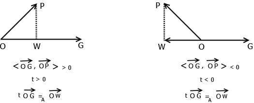
Figure 8.1. An illustration of Theorem 59, the existence of a point $W$ where $\left<\overrightarrow{WO},\overrightarrow{WP}\right>_{A}=0.$

Proof.

Let $O,G$ be two given points with $O\neq_{P}G$. Let $P$ be any point such that $P\notin l_{OG}$. We want to find $t\in\mathbb{R}$ where

(8.2) $$(t)\;\overrightarrow{OG}=_{A}\overrightarrow{OW},$$

for some $W\in l_{OG}$ which satisfies Equation (8.1). See Figure 8.1. By using Definition 4 we can rewrite Equation (8.2) as $-((t)\;\overrightarrow{OG})=_{A}\overrightarrow{WO}$. This means that Equation (8.1) is equivalent to

(8.3) $$\left<-((t)\;\overrightarrow{OG}),\overrightarrow{WP}\right>_{A}=0.$$

If $t=0$, then it follows by Definition 9 and Proposition 6 that $O=W$ and the preceding equation holds trivially. For $t\neq 0$, Definition 5, Equations (2.8) and (2.5) imply that

$$0 =\left<-((t)\;\overrightarrow{OG}),\overrightarrow{WP}\right>_{A}=-t\;\left<\overrightarrow{OG},\overrightarrow{WO}+_{A}\overrightarrow{OP}\right>_{A}$$

$$=-t\;\left<\overrightarrow{OG},\overrightarrow{WO}\right>_{A}-t\;\left<\overrightarrow{OG},\overrightarrow{OP}\right>_{A}$$

$$=-t\;\left<\overrightarrow{OG},-((t)\;\overrightarrow{OG})\right>_{A}-t\;\left<\overrightarrow{OG},\overrightarrow{OP}\right>_{A}$$

$$=t^{2}\;\left<\overrightarrow{OG},\overrightarrow{OG}\right>_{A}-t\;\left<\overrightarrow{OG},\overrightarrow{OP}\right>_{A}=0.$$

Solving the preceding equation for $t$ yields

(8.4) $$t=\frac{\left<\overrightarrow{OG},\overrightarrow{OP}\right>_{A}}{\left<\overrightarrow{OG},\overrightarrow{OG}\right>_{A}}.$$

The two quantities $\left<\overrightarrow{OG},\overrightarrow{OP}\right>_{A}$ and $\left<\overrightarrow{OG},\overrightarrow{OG}\right>_{A}$ are uniquely determined as $O,\;G$, and $P$ are fixed. Hence $t$ in Equation (8.4) is unique. Therefore, Equation (8.2) implies that there exists a unique point $W\in l_{OG}$ such that Equation (8.1) holds. ∎

Theorem 59 allows for a geometric proof of the arrow space Cauchy-Schwartz analog.

Theorem 60.

(Cauchy-Schwartz Inequality) Given $\overrightarrow{OG}$ and $\overrightarrow{AB}$ in $\mathcal{P}_{A}$,

(8.5) $$\left<\overrightarrow{OG},\overrightarrow{AB}\right>^{2}_{A}\leq\left<\overrightarrow{OG},\overrightarrow{OG}\right>_{A}\left<\overrightarrow{AB},\overrightarrow{AB}\right>_{A},$$

with equality holding in (8.5) if and only if $\overrightarrow{AB}=_{A}(s)\overrightarrow{OG}$ for some real number $s$.

Proof.

If $O=_{P}G$, the result is trivially true. So assume $O\neq_{P}G$ and let $l_{OG}$ be the line through the points $O$ and $G$. By Axiom 5, set $\overrightarrow{OP}$ to be the unique arrow such that $\overrightarrow{AB}\,\,\Re\,\,\overrightarrow{OP}$. Since Axiom 4 implies that $\left<\overrightarrow{OG},\overrightarrow{AB}\right>_{A}=\left<\overrightarrow{OG},\overrightarrow{OP}\right>_{A}$, we see (8.5) is equivalent to

(8.6) $$\left<\overrightarrow{OG},\overrightarrow{OP}\right>^{2}_{A}\leq\left<\overrightarrow{OG},\overrightarrow{OG}\right>_{A}\left<\overrightarrow{OP},\overrightarrow{OP}\right>_{A}.$$

Thus it suffices to verify (8.6).

If $P\in l_{OG}$, then $\overrightarrow{OP}=(s)\overrightarrow{OG}$ for some $s\in\mathbb{R}$. In this case

$$\left<\overrightarrow{OG},\overrightarrow{OP}\right>^{2}_{A} =\left<\overrightarrow{OG},(s)\overrightarrow{OG}\right>^{2}_{A}=s^{2}\left<\overrightarrow{OG},\overrightarrow{OG}\right>^{2}_{A}$$

$$=\left<\overrightarrow{OG},\overrightarrow{OG}\right>_{A}\left<(s)\overrightarrow{OG},(s)\overrightarrow{OG}\right>_{A}$$

$$=\left<\overrightarrow{OG},\overrightarrow{OG}\right>_{A}\left<\overrightarrow{OP},\overrightarrow{OP}\right>_{A}.$$

Now assume $P\notin l_{OG}$. Then by Theorem 59 there is a unique point $W\in l_{OG}$, namely $\overrightarrow{OW}=(t)\overrightarrow{OG}$ with $t=\frac{\left<\overrightarrow{OG},\overrightarrow{OP}\right>_{A}}{\left<\overrightarrow{OG},\overrightarrow{OG}\right>_{A}}$, such that $\left<\overrightarrow{WO},\overrightarrow{WP}\right>_{A}=0$. In other words, Triangle OPW is a right triangle with hypotenuse $\overrightarrow{OP}$; see Figure 8.1. The Pythagorean theorem implies that

$$\left<\overrightarrow{OP},\overrightarrow{OP}\right>_{A} =\left<\overrightarrow{OW},\overrightarrow{OW}\right>_{A}+\left<\overrightarrow{WP},\overrightarrow{WP}\right>_{A}$$

$$\geq\left<\overrightarrow{OW},\overrightarrow{OW}\right>_{A}=\left<(t)\overrightarrow{OG},(t)\overrightarrow{OG}\right>_{A}$$

$$=t^{2}\left<\overrightarrow{OG},\overrightarrow{OG}\right>_{A}=\frac{\left<\overrightarrow{OG},\overrightarrow{OP}\right>_{A}^{2}}{\left<\overrightarrow{OG},\overrightarrow{OG}\right>_{A}},$$

which after multiplication by $\left<\overrightarrow{OG},\overrightarrow{OG}\right>_{A}$ is equivalent to Inequality (8.6). ∎

Next we define the barycentric coordinates of a point $M$ in $\mathcal{P}$, a concept crucial to the definition of affine maps (see Definitions 2.2 and 2.6 of [10]). To do so we fix an origin $O$ in $\mathcal{P}$ and introduce the following definition

Definition 61.

Let $\left\{P_{i}\right\}_{i=1}^{i=n}$ be a set of points in $\mathcal{P}$ such that $[\overrightarrow{OM}]=\sum_{i=1}^{i=n}\;\lambda_{i}\;[\overrightarrow{OP_{i}}]$, where $\sum_{i=1}^{i=n}\;\lambda_{i}=1$. We write $M:=_{P}\sum_{i=1}^{i=n}\;\lambda_{i}\;P_{i}$ and call the real numbers $\lambda_{i}\geq 0,\;i=1,...,\;n$ the barycentric coordinates of a point $M$.

To show that Definition 61 is well defined and independent of the chosen origin, we need the following theorem.

Theorem 62.

Let $\{P_{i}\}_{i=1}^{n}$ be a family of distinct points in $\mathcal{P}$. Let $O$ be a coordinate free origin and $\{\lambda_{i}\}_{i=1}^{n}$ be a family of real numbers such that $\sum_{i=1}^{n}\lambda_{i}=1$. There exists a unique point $M$ such that $\sum_{i=1}^{n}[(\lambda_{i})\;\overrightarrow{OP_{i}}]=_{V}[\overrightarrow{OM}]$. Moreover, the point $M$ is independent from the choice of $O$. That is, if $\tilde{O}$ is any other point and if

(8.7) $$\sum_{i=1}^{n}[(\lambda_{i})\;\overrightarrow{\tilde{O}P_{i}}]=_{V}[\overrightarrow{\tilde{O}L}],$$

then we must have $L=_{P}M$. See Figure 8.2.

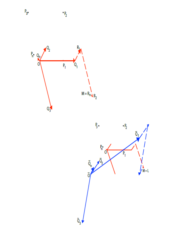
Figure 8.2. The top figure with the red arrows illustrates the barycenter from $O$ while the bottom figure with blue arrows represents the barycenter from $\tilde{O}$.

Proof.

Let $(\lambda_{i})\;\overrightarrow{OP_{i}}=_{A}\overrightarrow{OQ_{i}}$, $1\leq i\leq n$, for some points $\{Q_{i}\}_{i=1}^{n}$. The existence and uniqueness of a point $M$, such that

(8.8) $$\sum_{i=1}^{n}[(\lambda_{i})\;\overrightarrow{OP_{i}}]=_{V}\sum_{i=1}^{n}(\lambda_{i})[\overrightarrow{OP_{i}}]=_{V}\sum_{i=1}^{n}[\overrightarrow{OQ_{i}}]=_{V}[\overrightarrow{OM}],$$

follows from $n-1$ applications Definition 45 as follows

$$(n-1)\;\text{times}\;\begin{cases}[\overrightarrow{OQ_{1}}]+_{V}[\overrightarrow{OQ_{2}}]=_{V}[\overrightarrow{OQ_{1}}+_{A}\overrightarrow{Q_{1}R_{1}}]=_{V}[\overrightarrow{OR_{1}}],\\ {}[\overrightarrow{OR_{1}}]+_{V}[\overrightarrow{OQ_{3}}]=_{V}[\overrightarrow{OR_{1}}+_{A}\overrightarrow{R_{1}R_{2}}]=_{V}[\overrightarrow{OR_{2}}],\\ :\\ {}[\overrightarrow{OR_{n-2}}]+_{V}[\overrightarrow{OQ_{n}}]=_{V}[\overrightarrow{OR_{n-2}}+_{A}\overrightarrow{R_{n-2}M}]=_{V}[\overrightarrow{OM}],\end{cases}$$

where $\{R_{i}\}_{i=1}^{n-1}$ (we put $M=R_{n-1}$) are the unique points that we get when we apply Axiom 5 in Definition 45. See Figure 8.3.

Figure 8.3. $\sum_{i=1}^{n}[(\lambda_{i})\;\overrightarrow{OP_{i}}]=_{V}\sum_{i=1}^{n}[\overrightarrow{OQ_{i}}]=_{V}[\overrightarrow{OM}],\;n=4$

To show that $M$ is independent of the choice of $O$ notice that by Definitions 5 and Theorem 57 (1) we have

(8.9) $$[\overrightarrow{OM}]=_{V}\sum_{i=1}^{n}\lambda_{i}[\overrightarrow{OP_{i}}]=_{V}\sum_{i=1}^{n}\lambda_{i}[\overrightarrow{O\tilde{O}}+_{A}\overrightarrow{\tilde{O}P_{i}}]=_{V}[\overrightarrow{O\tilde{O}}]\sum_{i=1}^{n}\lambda_{i}+_{V}\sum_{i=1}^{n}\lambda_{i}[\overrightarrow{\tilde{O}P_{i}}],$$

for any point $\tilde{O}$ other than $O$. Since $\sum_{i=1}^{n}\lambda_{i}=1$, by Theorem 56(2) and Equations (8.8) and (8.9) we find that

(8.10) $$[\overrightarrow{OM}]=_{V}[\overrightarrow{O\tilde{O}}]+_{V}[\overrightarrow{\tilde{O}L}]=_{V}[\overrightarrow{O\tilde{O}}+_{A}\overrightarrow{\tilde{O}L}]=_{V}[\overrightarrow{OL}],$$

where $[\overrightarrow{\tilde{O}L}]=_{V}\sum_{i=1}^{n}(\lambda_{i})[\overrightarrow{\tilde{O}P_{i}}]$ for some point $L$. This means that $\overrightarrow{OL}\;\Re\;\overrightarrow{OM}$ which implies by Definition 41 and Proposition 21 that $L=_{P}M$, as desired. ∎

References

- [1] H. Anton, Elemetary Linear Algebra. 9. ed. J. Wiley 2005.
- [2] T. M. Apostol, Calculus. 2nd ed. Waltham, Mass. Blaisdell Pub 1967.
- [3] S. Axler, Linear Algebra Done Right. Third Edition. Springer International Publishing 2015.
- [4] D. D. Berkey, Calculus. 2nd ed. New York. Saunders College Pub 1988.
- [5] L. Bers, F. Karal, Calculus. 2nd ed. New York. Holt, Rinehart and Winston 1976.
- [6] R. C. Buck, E. F. Buck, Advanced Calculus. 2nd ed. New York. McGraw-Hill 1965.
- [7] M. J. Crowe, A History of Vector Analysis: The Evolution of the Idea of a Vectorial System. Notre Dame. University of Notre Dame Press 1967.
- [8] K. O. Friedrichs, From Pythagoras to Einstein, The Mathematical Association of America 1965.
- [9] J. Gallier, J. Quaintance, Algebra, Topology, Differential Calculus, and Optimization Theory For Computer Science and Engineering 2019.
- [10] J. Gallier, J. Quaintance, Aspects of Convex Geometry Polyhedra, Linear Programming, Shellings, Voronoi Diagrams, Delaunay Triangulations 2017.
- [11] L. L. Severance, The Theory of Equipollences: Method of Analytical Geometry of Sig. Bellavitis. Meadville, Pa. Tribune 1930.
- [12] J. Stewart, Essential Calculus: Early Transcendentals. Belmont, CA. Thomson Higher Education 2007.