Numerical Approximation of Partial Differential Equations by a Variable Projection Method with Artificial Neural Networks

Abstract

We present a method for solving linear and nonlinear partial differential equations (PDE) based on the variable projection framework and artificial neural networks. For linear PDEs, enforcing the boundary/initial value problem on the collocation points gives rise to a separable nonlinear least squares problem about the network coefficients. We reformulate this problem by the variable projection approach to eliminate the linear output-layer coefficients, leading to a reduced problem about the hidden-layer coefficients only. The reduced problem is solved first by the nonlinear least squares method to determine the hidden-layer coefficients, and then the output-layer coefficients are computed by the linear least squares method. For nonlinear PDEs, enforcing the boundary/initial value problem on the collocation points gives rise to a nonlinear least squares problem that is not separable, which precludes the variable projection strategy for such problems. To enable the variable projection approach for nonlinear PDEs, we first linearize the problem with a Newton iteration, using a particular linearization formulated in terms of the updated approximation field. The linearized system is solved by the variable projection framework together with artificial neural networks. Upon convergence of the Newton iteration, the neural-network coefficients provide the representation of the solution field to the original nonlinear problem. We present ample numerical examples with linear and nonlinear PDEs to demonstrate the performance of the method developed herein. For smooth field solutions, the errors of the current method decrease exponentially as the number of collocation points or the number of output-layer coefficients increases. We compare extensively the current method with the extreme learning machine (ELM) method from a previous work. Under identical conditions and network configurations, the current method exhibits an accuracy significantly superior to the ELM method.

Keywords: artificial neural networks, variable projection, linear least squares, nonlinear least squares, scientific machine learning, deep learning

1 Introduction

This work concerns the numerical approximation of partial differential equations (PDE) with artificial neural networks (ANN), and we explore the use of the variable projection (VarPro) approach GolubP1973 ; GolubP2003 together with ANNs for solving linear and nonlinear PDEs. Neural network-based PDE solvers, especially those based on deep neural networks (DNN) and deep learning GoodfellowBC2016 , have flourished in the past few years; see e.g. SirignanoS2018 ; RaissiPK2019 ; EY2018 ; HeX2019 ; LuoY2020 ; ZangBYZ2020 ; DongN2020 ; Samaniegoetal2020 ; WangYP2020 ; MaoJK2020 ; LuMMK2021 ; LiangJHY2021 , and the recent review Karniadakisetal2021 and the references therein. The DNN-based PDE solvers are fairly straightforward to implement, by encoding the PDEs, the boundary and initial conditions into a cost function and then using some flavor of gradient descent (or back propagation) type optimization algorithms to minimize this cost. Their weakness lies in the limited accuracy and the high computational cost (long network-training time). Another promising class of neural network-based methods for computational PDEs has recently appeared DongL2021 ; DongL2021bip ; DwivediS2020 ; FabianiCRS2021 ; DongY2021 , which are based on a type of randomized neural networks called extreme learning machines (ELM) HuangZS2006 ; HuangCS2006 . With these methods the weight/bias coefficients in the hidden layers of the neural network are set to random values and are fixed. Only the coefficients of the linear output layer are trainable, and they are trained by a linear least squares method for linear PDEs and by a nonlinear least squares method for nonlinear PDEs DongL2021 . It has been shown in DongL2021 that the accuracy and the computational cost (network training time) of the ELM-based method are considerably superior to those of the aforementioned DNN-based PDE solvers. In addition, the computational performance of the ELM-type method from DongL2021 is observed to be comparable to or exceed that of the classical finite element method (FEM). Further extensions and improvements to the ELM method of DongL2021 have been documented in DongY2021 recently, which compares systematically the improved method with the classical and high-order FEM for solving a number of linear and nonlinear PDEs. The improved ELM method outperforms the classical second-order FEM by a considerable margin, and it outcompetes the high-order FEM when the problem size is not very small DongY2021 .

Variable projection (VarPro) is a classical approach for solving separable nonlinear least squares (SNLLS) problems GolubP1973 ; GolubP2003 . These problems are separable in the sense that the unknown parameters or variables can be separated into two sets: the linear parameters and the nonlinear parameters. Problems of this kind often involve a model function that is a linear combination of parameterized nonlinear basis functions. The basic idea of VarPro is to treat the linear parameters as dependent on the nonlinear parameters, and then eliminate the linear parameters from the problem by using the linear least squares method. This gives rise to a reduced, but generally more complicated, nonlinear least squares problem that involves only the nonlinear parameters GolubP2003 . One can then solve the reduced problem for the nonlinear parameters by a nonlinear least squares method, typically involving a Gauss-Newton type algorithm coupled with trust region or backtracking line search strategies DennisS1996 ; Bjorck2015 . Upon attaining the nonlinear parameters, one then computes the linear parameters by the linear least squares method. Although the reduced problem is in general more complicated, the benefits of variable projection are typically very significant. These include the reduced dimension of the parameter space, better conditioning, and faster convergence with the reduced problem RuheW1980 ; SjobergV1997 ; GolubP2003 . In some sense the idea of variable projection to least squares problems can be analogized to the Schur complement in linear algebra or the static condensation in computational mechanics (see e.g. KarniadakisS2005 ).

The VarPro algorithm was originally developed in GolubP1973 , and has been improved and generalized by a number of researchers and applied to many areas in the past few decades Kaufman1975 ; RuheW1980 ; GolubP2003 ; ChungHN2006 ; Osborne2007 ; MullenS2009 ; OlearyR2013 ; AskhamK2018 ; ChenGCL2019 ; SongXHZ2020 ; ErichsonZMBKA2020 ; LeeuwenA2021 ; NewmanCCR2021 . In GolubP1973 the authors have proved the equivalence between the solution of the VarPro reduced formulation and that of the original problem, and developed differentiation formulas for the orthogonal projectors and the Moore-Penrose pseudoinverses, which are critical to the computation of the Jacobian matrix in the nonlinear least squares solution of the reduced problem. An important simplification to the VarPro algorithm is suggested in Kaufman1975 , which involves computing an approximate Jacobian rather than the true Jacobian. This significantly reduces the per-iteration cost of VarPro, with generally insignificant or negligible sacrifice to the accuracy for many problems GanCCC2018 . The variable projection algorithms for problems with constraints on the linear or nonlinear parameters are investigated in e.g. KaufmanP1978 ; SimaH2007 ; OlearyR2013 ; CornelioPN2014 , among others. The implementations of the VarPro method have been discussed in Krogh1974 ; OlearyR2013 . In GolubP2003 the original developers of VarPro have reviewed the developments of this method up to the early 2000s and compiled an extensive list of areas for its ongoing and potential applications. A generalization of the variable projection approach has been considered in RuheW1980 , which deals with two separate classes of variables without requiring one class to be linear; see also more recent contributions on the generalization of VarPro in e.g. AravkinL2012 ; ShearerG2013 ; HerringNR2018 ; LeeuwenA2021 . We would also like to mention the simplification of the Jacobian matrix in RuanoJF1991 , and the algorithm of McLooneBI1998 , which resembles the variable projection approach in some sense; see a comparison of these algorithms with the variable projection method in GanCCC2018 . An approach related to variable projection is the so-called block coordinate descent NocedalW1999 , which alternates between the minimization of two separate sets of variables involved in the problem RuheW1980 ; ChungHN2006 ; CyrGPPT2020 .

The VarPro algorithm or its variants for training neural networks have been the subject of several studies in the literature WeiglB1993 ; WeiglGB1993 ; WeiglB1994 ; SjobergV1997 ; PereyraSW2006 ; KimL2008 ; NewmanRHW2020 ; NewmanCCR2021 . The projection learning algorithm developed in WeiglB1993 ; WeiglGB1993 ; WeiglB1994 is in the same spirit as variable projection, and it computes the linear parameters by the linear least squares method and the nonlinear parameters by a gradient descent scheme. In SjobergV1997 the authors have proved that the reduced nonlinear functional of the variable projection approach, while seemingly more complicated, leads to a better-conditioned problem and always converges faster than the original problem; see also RuheW1980 . The VarPro method together with the Levenberg-Marquardt algorithm is employed for the training of two-layered neural networks in PereyraSW2006 ; KimL2008 and compared with other related approaches. In the recent works NewmanRHW2020 ; NewmanCCR2021 the authors extend the variable projection approach to deal with non-quadratic objective functions, such as the cross-entropy function in classification tasks, and also present a stochastic optimization method (termed “slimTrain”) based on variable projection for training deep neural networks with attractive properties.

In the current work we focus on the variable projection approach for solving partial differential equations. We numerically approximate the solution fields to linear and nonlinear PDEs by exploiting variable projection together with artificial neural networks. For computational PDEs, the issues one would encounter with VarPro are a little different from those for data fitting problems or function approximations, which account for the majority of applications the VarPro algorithm is developed for in the literature. For solving PDEs, we do not have the data for the field function to be solved for, unlike in data fitting problems. What we do have are the conditions (or constraints) the solution field needs to satisfy, namely, the PDEs, the boundary conditions, and also the initial conditions if the problem is time-dependent. In order to deal with this type of problems, the variable projection method needs to be adapted accordingly.

The general approach with VarPro and artificial neural networks for solving PDEs is as follows. We employ a feed-forward neural network with one or more hidden layers to represent the field solution to the PDE, requiring that the output layer be linear (i.e. applying no activation function) and with zero bias. We enforce the PDEs on a set of collocation points in the domain, and enforce the boundary/initial conditions on a set of collocation points on the appropriate boundaries of the spatial (or spatial-temporal) domain. This gives rise to a set of discrete equations about the field function to be solved for, which depends on the weight/bias coefficients in the output/hidden layers of the neural network. In turn, this set of equations leads to a nonlinear least squares problem about the neural-network coefficients, providing an opportunity for the variable projection method if this nonlinear least squares problem is separable.

It is necessary to distinguish two types of linearities (or nonlinearities) before the variable projection approach can be used to solve the above nonlinear least squares problem. The first type concerns whether the neural-network coefficients are linear (or nonlinear) with respect to the output field of the network. Since no activation function is applied to the output layer, the output-layer coefficients are linear and the hidden-layer coefficients are nonlinear with respect to the network output. The second type concerns whether the boundary/initial value problem with the given PDE is linear (or nonlinear) with respect to the field function to be solved for.

If the boundary/initial problem is linear, i.e. both the PDE and the boundary/initial conditions are linear with respect to the solution field, then the aforementioned nonlinear least squares problem is separable. The output-layer coefficients of the neural network are the linear parameters and the hidden-layer coefficients are the nonlinear parameters in this separable nonlinear least squares problem. In this case, employing the VarPro approach for training the neural network to solve the given boundary/initial value problem would be conceptually straightforward.

On the other hand, if the boundary/initial value problem is nonlinear, i.e. either the PDE itself or the associated boundary/initial conditions are nonlinear with respect to the solution field, the aforementioned nonlinear least squares problem is not separable. In this case all the weight/bias coefficients in the neural network become nonlinear parameters in the aforementioned nonlinear least squares problem. Therefore, the variable projection approach cannot be directly used for solving nonlinear PDEs (or problems with nonlinear boundary/initial conditions). How to enable the variable projection method to solve nonlinear PDEs is the focus of the current work.

In this paper we present a Newton-variable projection method together with artificial neural networks for solving nonlinear boundary/initial value problems (nonlinear PDEs or nonlinear boundary/initial conditions). Given a nonlinear boundary/initial value problem, we first linearize the problem for the Newton iteration, with a particular linearized form. More specifically, the linearization is formulated in terms of the updated approximation field, not the increment field. This linearization form is critical to the accuracy of the current Newton-VarPro method. The linearized system (PDE and boundary/initial conditions) is linear with respect to the updated approximation field, and it is solved by the variable projection approach together with the neural networks. Therefore, to solve nonlinear PDEs, the current method involves an overall Newton iteration. Within each iteration, we use the VarPro method together with ANNs to solve the linearized system to attain the updated field approximation. Upon convergence of the Newton iteration, the weight/bias coefficients of the neural network contain the representation of the solution field to the original nonlinear problem.

The VarPro method together with ANNs for solving linear PDEs has been considered first in this paper. We discuss in some detail how to implement the Jacobian matrix together with neural networks, and how to introduce perturbations in VarPro when solving the reduced problem in order to prevent the solution from being trapped to the local minima in the nonlinear least squares computation. We have presented a number of numerical examples, involving both linear and nonlinear PDEs, to test the performance of the VarPro method developed here. We observe that, for smooth field solutions, the VarPro errors decrease exponentially as the number of collocation points or the number of output-layer coefficients in the neural network increases, which is reminiscent of the spectral convergence of traditional high-order methods KarniadakisS2005 ; SzaboB1991 ; ZhengD2011 ; DongS2012 ; Dong2018 ; Dong2015clesobc ; LinYD2019 ; YangD2019 ; YangD2020 . We also compare extensively the performance of the current VarPro method with that of the ELM method from DongL2021 ; DongY2021 . The numerical results show that, under identical conditions and network configurations, the VarPro method is considerably more accurate than the ELM method, especially when the size of the neural network is small. On the other hand, the computational cost (i.e. network training time) of the VarPro method is usually much higher than that of the ELM method.

In the current work the VarPro method and the neural networks are implemented based on the Tensorflow (www.tensorflow.org) and Keras (keras.io) libraries in Python. The scipy and numpy libraries in Python are used for the linear and nonlinear least squares computations. All the numerical tests are carried out on a MAC computer in the authors’ institution.

The main contribution of this paper lies in the Newton-VarPro method together with artificial neural networks for solving nonlinear partial differential equations. To the best of the authors’ knowledge, this work seems also to be the first time when the variable projection approach (with ANNs) is extended and adapted to solving linear partial differential equations.

The rest of this paper is structured as follows. In Section 2 we first outline how to solve linear PDEs with the variable projection approach together with ANNs. The computations for the reduced residual function and the Jacobian matrix of the reduced problem, and the VarPro algorithm with perturbations are discussed in detail. Then we introduce the Newton-VarPro method together with ANNs for solving nonlinear PDEs. In Section 3 we present several numerical examples with linear and nonlinear PDEs to demonstrate the accuracy of the VarPro method developed herein. The performance of the current VarPro method is compared extensively with that of the ELM method from DongL2021 ; DongY2021 . Section 4 then concludes the presentation with some closing remarks and comments on the presented method.

2 Variable Projection with Artificial Neural Networks for Computational PDEs

We develop an algorithm combining the variable projection (VarPro) framework with artificial neural networks (ANN) for numerically approximating PDEs. For linear PDEs, the ANN representation of the solution field leads to a separable nonlinear least squares problem, which can be solved by the variable projection approach. For nonlinear PDEs, on the other hand, the ANN representation of the solution field leads to a nonlinear least squares (NLLSQ) problem that is not separable, preventing the use of the variable projection strategy. We overcome this issue by a combined Newton-variable projection method, which enables the variable projection approach in solving nonlinear PDEs. In the following subsections we first illustrate the VarPro/ANN algorithm for solving linear PDEs, and then introduce the Newton-VarPro/ANN algorithm for solving nonlinear PDEs.

2.1 Variable Projection Method for Solving Linear PDEs

Consider a domain $\Omega\subset\mathbf{R}^{d}$ ($d=1$ to $3$) and the following linear boundary-value problem on $\Omega$,

$$Lu=f(\mathbf{x}),$$ (1a)

$$Bu=g(\mathbf{x}),\quad\text{on}\ \partial\Omega.$$ (1b)

In these equations $\mathbf{x}=(x_{1},\dots,x_{d})$ denotes the coordinate, $u(\mathbf{x})$ is the field solution to be solved for, $L$ denotes a linear differential operator, $B$ denotes a linear algebraic or differential operator on the boundary $\partial\Omega$ representing the boundary conditions, and $f(\mathbf{x})$ and $g(\mathbf{x})$ are prescribed non-homogeneous terms in the domain or on the boundary. We assume that $L$ may include linear differential operators with respect to the time $t$ (e.g. $\frac{\partial}{\partial t}$, $\frac{\partial^{2}}{\partial t^{2}}$). In such a case, this becomes an initial boundary-value problem, and we treat the time $t$ in the same way as the spatial coordinates. We designate the last coordinate $x_{d}$ as $t$, and $\Omega$ becomes a spatial-temporal domain. Accordingly, we assume that the boundary condition (1b) in this case should include appropriate initial condition(s) with respect to $t$, which will be imposed only on the portion of $\partial\Omega$ corresponding to the initial condition(s). The point here is that the equations (1a)–(1b) may denote a time-dependent problem, and we will not distinguish the stationary and time-dependent cases in the following discussions. We assume that the problem (1) is well-posed.

We approximate the solution field $u(\mathbf{x})$ by a feed-forward neural network GoodfellowBC2016 with $(L+1)$ layers, where $L$ is an integer satisfying $L\geqslant 2$. The input layer (layer $0$) of the neural network contains $d$ nodes which represent the coordinate $\mathbf{x}$, and the output layer (layer $L$) contains $1$ node which represents the solution $u$. The $(L-1)$ layers in between are the hidden layers. From layer to layer the network logic represents an affine transform followed by a node-wise function composition with an activation function $\sigma(\cdot)$ GoodfellowBC2016 . The coefficients of the affine transforms are referred to as the weight and bias coefficients of the neural network. For the convenience of presentation, we use the vector $[M_{0},M_{1},\dots,M_{L}]$ to denote the architecture of the neural network, where $M_{i}$ ($0\leqslant i\leqslant L$) denotes the number of nodes in layer $i$, with $M_{0}=d$ and $M_{L}=1$. We also use $M=M_{L-1}$ to denote the number of nodes in the last hidden layer in what follows. The weight/bias coefficients in all the hidden layers and in the output layer are the trainable parameters of the neural network.

In the current work, we make the assumption that the output layer contains no bias (or zero bias), and no activation function (or equivalently it uses the identity activation function $\sigma(x)=x$). So the output layer of the neural network is linear in this paper.

Let $\Phi_{j}(\bm{\theta},\mathbf{x})$ ($1\leqslant j\leqslant M$) denote the output fields of the last hidden layer, where $\bm{\theta}=(\theta_{1},\dots,\theta_{N_{h}})^{T}$ denotes the vector of weight/bias coefficients in all the hidden layers of the network, with $N_{h}=\sum_{i=1}^{L-1}M_{i}(M_{i-1}+1)$. Then we have the following expansion relation,

$$u(\mathbf{x})=\sum_{j=1}^{M}\beta_{j}\Phi_{j}(\bm{\theta},\mathbf{x})=\bm{\Phi}(\bm{\theta},\mathbf{x})\bm{\beta}$$ (2)

where $\bm{\Phi}(\bm{\theta},\mathbf{x})=[\Phi_{1}(\bm{\theta},\mathbf{x}),\dots,\Phi_{M}(\bm{\theta},\mathbf{x})]$ denotes the set of output fields of the last hidden layer, and $\bm{\beta}=[\beta_{1},\dots,\beta_{M}]^{T}$ is the vector of weight coefficients of the output layer. Note that $(\bm{\theta},\bm{\beta})$ are the trainable parameters of the neural network. Note also that $M$ represents the number of nodes in the last hidden layer, as well as the number of output-layer coefficients.

We choose a set of $N$ ($N\geqslant 1$) collocation points on $\Omega$, which can be chosen according to a certain distribution (e.g. random, uniform). Among them $N_{b}$ ($1\leqslant N_{b}\leqslant N-1$) collocation points reside on the boundary $\partial\Omega$, and the rest of the points are from the interior of $\Omega$. We use $\mathbb{X}$ to denote the set of all the collocation points and $\mathbb{X}_{b}$ to denote the set of collocation points on $\partial\Omega$. In the current paper, for simplicity we assume that $\Omega$ is a rectangular domain, given by the interval $[a_{i},b_{i}]$ ($1\leqslant i\leqslant d$) in the $i$-th direction. We employ a uniform set of grid points (including the boundary end points) in each direction as the collocation points for the numerical tests in Section 3.

The input training data to the neural network consist of the coordinates of the all the $N$ collocation points on $\Omega$. We use the $N\times d$ matrix $\mathbf{X}$ to denote the input data. Each row of $\mathbf{X}$ denotes the coordinates a collocation point. Let the $N\times 1$ matrix $\mathbf{U}$ (column vector) denote the output data of the neural network, which represents the solution field $u(\mathbf{x})$ evaluated on all the $N$ collocation points. We use the $N\times M$ matrix $\bm{\Psi}$ to denote the output data of the last hidden layer of the neural network, which represents the output fields $\bm{\Phi}(\bm{\theta},\mathbf{x})$ of the last hidden layer evaluated on all the $N$ collocation points.

Inserting the expansion (2) into (1), and enforcing the equation (1a) on all the collocation points from $\mathbb{X}$ and the equation (1b) on all the boundary collocation points from $\mathbb{X}_{b}$, we arrive at the following system,

$$\sum_{j=1}^{M}\left[L\Phi_{j}(\bm{\theta},\mathbf{x}_{p})\right]\beta_{j}=f(\mathbf{x}_{p}),\quad 1\leqslant p\leqslant N,\ \text{where}\ \mathbf{x}_{p}\in\mathbb{X},$$ (3a)

$$\sum_{j=1}^{M}\left[B\Phi_{j}(\bm{\theta},\mathbf{x}_{q})\right]\beta_{j}=g(\mathbf{x}_{q}),\quad 1\leqslant q\leqslant N_{b},\ \text{where}\ \mathbf{x}_{q}\in\mathbb{X}_{b}.$$ (3b)

This is a system of $(N+N_{b})$ algebraic equations about the trainable parameters $(\bm{\theta},\bm{\beta})$, with $(N_{h}+M)$ unknowns. Note that for a given $\bm{\theta}$ the terms $L\Phi_{j}(\bm{\theta},\mathbf{x}_{p})$ and $B\Phi_{j}(\bm{\theta},\mathbf{x}_{q})$ in the above equations can be computed by forward evaluations of the neural network and auto-differentiations.

We seek a least squares solution for $(\bm{\theta},\bm{\beta})$ to the system (3). This system is linear with respect to $\bm{\beta}$, and nonlinear with respect to $\bm{\theta}$. This leads to a separable nonlinear least squares problem. Therefore we adopt the variable projection approach GolubP1973 for the least squares solution of the system (3).

To make the formulation more compact, we re-write the system (3) into a matrix form,

$$\mathbf{H}(\bm{\theta})\bm{\beta}=\mathbf{S},\ \ \text{where}\ \ \mathbf{H}(\bm{\theta})=\begin{bmatrix}\vdots\\ L\bm{\Phi}(\bm{\theta},\mathbf{x}_{p})\\ \vdots\\ \hdashline[1pt/1pt]\vdots\\ B\bm{\Phi}(\bm{\theta},\mathbf{x}_{q})\\ \vdots\end{bmatrix}_{(N+N_{b})\times M},\ \ \mathbf{S}=\begin{bmatrix}\vdots\\ f(\mathbf{x}_{p})\\ \vdots\\ \hdashline[1pt/1pt]\vdots\\ g(\mathbf{x}_{q})\\ \vdots\end{bmatrix}_{(N+N_{b})\times 1}.$$ (4)

For any given $\bm{\theta}$, the least squares solution for the linear parameters $\bm{\beta}$ to this system is given by

$$\bm{\beta}=\left[\mathbf{H}(\bm{\theta})\right]^{+}\mathbf{S},$$ (5)

where the superscript in $\mathbf{H}^{+}$ denotes the Moore-Penrose pseudo-inverse of $\mathbf{H}$. Define the residual function of the system (4) by

$$\mathbf{r}(\bm{\theta})=\mathbf{H}(\bm{\theta})\bm{\beta}-\mathbf{S}=\mathbf{H}(\bm{\theta})\mathbf{H}^{+}(\bm{\theta})\mathbf{S}-\mathbf{S},$$ (6)

where the linear parameter $\bm{\beta}$ has been eliminated by using equation (5). We compute the optimal nonlinear parameters $\bm{\theta}_{opt}$ by minimizing the Euclidean norm of the residual function $\mathbf{r}$,

$$\bm{\theta}_{opt}=\operatorname*{arg\,min}_{\bm{\theta}}\frac{1}{2}\|\mathbf{r}(\bm{\theta})\|^{2}=\operatorname*{arg\,min}_{\bm{\theta}}\frac{1}{2}\|\mathbf{H}(\bm{\theta})\mathbf{H}^{+}(\bm{\theta})\mathbf{S}-\mathbf{S}\|^{2},$$ (7)

where $\|\cdot\|$ denotes the Euclidean norm. After $\bm{\theta}_{opt}$ is obtained, we can compute the optimal linear parameters $\bm{\beta}_{opt}$ based on equation (5) or by solving equation (4) using the linear least squares method. Outlined above is the essence of the variable projection approach for solving the system (3) for $(\bm{\theta},\bm{\beta})$.

The problem represented by (7) is a nonlinear least squares problem about $\bm{\theta}$ only, where the linear parameter $\bm{\beta}$ has been eliminated. We solve this problem by a Gauss-Newton algorithm combined with a trust region strategy. Specifically, in the current paper we solve this problem by employing the nonlinear least squares library routine “scipy.optimize.least_squares” from the scipy package in Python, which implements the Gauss-Newton method together with a trust region reflective algorithm BranchCL1999 ; ByrdSS1988 .

input : $\bm{\theta}$; input data $\mathbf{X}$ to neural network; source data $\mathbf{S}$.

output : $\mathbf{r}(\bm{\theta})$.

1 update the hidden-layer coefficients of the neural network by $\bm{\theta}$

2 if $\bm{\theta}=\bm{\theta}_{s}$ then

3       retrieve $\mathbf{H}(\bm{\theta}_{s})$, and set $\mathbf{H}(\bm{\theta})=\mathbf{H}(\bm{\theta}_{s})$

4       retrieve $\bm{\beta}^{LS}(\bm{\theta}_{s})$, and set $\bm{\beta}^{LS}(\bm{\theta})=\bm{\beta}^{LS}(\bm{\theta}_{s})$

5      

6else

7       compute $\mathbf{H}(\bm{\theta})$ using the input data $\mathbf{X}$

8       solve equation (4) by the linear least squares method to get $\bm{\beta}^{LS}(\bm{\theta})$

9       set $\bm{\theta}_{s}=\bm{\theta}$, and save $\mathbf{H}(\bm{\theta})$ and $\bm{\beta}^{LS}(\bm{\theta})$

10      

11 end if

12

13compute $\mathbf{r}(\bm{\theta})$ by equation (8)

14

Algorithm 1 Computing the residual $\mathbf{r}(\bm{\theta})$

The scipy routine “least_squares()” requires two functions as input, which are needed by the Gauss-Newton algorithm. These are, for any given $\bm{\theta}$,

• a function for computing the residual $\mathbf{r}(\bm{\theta})$, and

• a function for computing the Jacobian matrix $\frac{\partial\mathbf{r}}{\partial\bm{\theta}}$.

The computation for $\mathbf{r}(\bm{\theta})$ is straightforward. For a given $\bm{\theta}$, we first solve equation (4) by the linear least squares method for the minimum-norm least squares solution $\bm{\beta}^{LS}$. Then we compute the residual according to equation (6) as follows,

$$\mathbf{r}(\bm{\theta})=\mathbf{H}(\bm{\theta})\bm{\beta}^{LS}-\mathbf{S}.$$ (8)

Note that the Moore-Penrose inverse $\mathbf{H}^{+}(\bm{\theta})$ is not explicitly computed in the implementation. In the current paper we employ the linear least squares routine “scipy.linalg.lstsq” from scipy to solve (4) for $\bm{\beta}^{LS}$. The computation for $\mathbf{r}(\bm{\theta})$ is summarized in the Algorithm 1.

Remark 2.1.

Let us elaborate on, for a given $\bm{\theta}$ and the input data $\mathbf{X}$, how to compute the matrix $\mathbf{H}(\bm{\theta})$ on line $6$ of Algorithm 1. As defined in (4), $H(\bm{\theta})$ consists of the terms $L\bm{\Phi}(\bm{\theta},\mathbf{x}_{p})$ ($\mathbf{x}_{p}\in\mathbb{X}$) and $B\bm{\Phi}(\bm{\theta},\mathbf{x}_{q})$ ($\mathbf{x}_{q}\in\mathbb{X}_{b}$). These terms involve the output fields of the last hidden layer $\bm{\Phi}(\bm{\theta},\mathbf{x})$, and their derivatives up to a certain order, evaluated on all the collocation points. All these terms can be computed by evaluating the neural network on the input data $\mathbf{X}$ and by auto-differentiations. Specifically, in our implementation we have created a sub-model to the neural network in Keras, with the neural network’s input as its input and with the output of the neural network’s last hidden layer as the sub-model’s output. Let us refer to this sub-model as the last-hidden-layer-model. Let $m$ denote the order of the PDE (1a), and we assume that the hidden-layer coefficients have been updated by the given $\bm{\theta}$. Then computing $\mathbf{H}(\bm{\theta})$ involves the the following procedure:

1. evaluate the last-hidden-layer-model on the input $\mathbf{X}$ to get $\bm{\Phi}(\bm{\theta},\mathbf{x})$ on all the collocation points;

2. compute the derivatives of $\bm{\Phi}(\bm{\theta},\mathbf{x})$ with respect to $\mathbf{x}$, up to the order $m$, on all the collocation points by a forward-mode auto-differentiation;

3. compute $L\bm{\Phi}(\bm{\theta},\mathbf{x})$ on all the collocation points based on the data for $\bm{\Phi}(\bm{\theta},\mathbf{x})$ and its derivatives;

4. extract the boundary data (i.e. on the boundary collocation points) for $\bm{\Phi}(\bm{\theta},\mathbf{x})$ and its derivatives from those data attained from steps (i) and (ii);

5. compute $B\bm{\Phi}(\bm{\theta},\mathbf{x})$ based on the boundary data for $\bm{\Phi}(\bm{\theta},\mathbf{x})$ and its derivatives;

6. assemble $L\bm{\Phi}(\bm{\theta},\mathbf{x})$ (on all the collocation points) and $B\bm{\Phi}(\bm{\theta},\mathbf{x})$ (on the boundary collocation points) to form $\mathbf{H}(\bm{\theta})$ based on equation (4).

Note that we employ the forward-mode auto-differentiations to compute the derivatives of $\bm{\Phi}(\bm{\theta},\mathbf{x})$ in step (ii) above, because the number of nodes in the last hidden layer ($M$) is typically much larger than that in the input layer ($d$). In this case the forward-mode auto-differentiation is significantly faster than the reverse-mode auto-differentiation. In our implementation we have used the “ForwardAccumulator” from the Tensorflow library for the forward-mode auto-differentiations.

For computing the Jacobian matrix $\frac{\partial\mathbf{r}}{\partial\bm{\theta}}$ we consider the following formula, which is due to GolubP1973 ,

$$\begin{split}\frac{\partial\mathbf{r}}{\partial\bm{\theta}}=&\left[\mathbf{I}-\mathbf{H}(\bm{\theta})\mathbf{H}^{+}(\bm{\theta})\right]\frac{\partial\mathbf{H}}{\partial\bm{\theta}}\mathbf{H}^{+}(\bm{\theta})\mathbf{S}\ +\ \left[\mathbf{H}^{+}(\bm{\theta})\right]^{T}\frac{\partial\mathbf{H}^{T}}{\partial\bm{\theta}}\left[\mathbf{I}-\mathbf{H}(\bm{\theta})\mathbf{H}^{+}(\bm{\theta})\right]\mathbf{S}\\ \approx&\left[\mathbf{I}-\mathbf{H}(\bm{\theta})\mathbf{H}^{+}(\bm{\theta})\right]\frac{\partial\mathbf{H}}{\partial\bm{\theta}}\mathbf{H}^{+}(\bm{\theta})\mathbf{S},\end{split}$$ (9)

where $\mathbf{I}$ denotes the identity matrix and equation (6) has been used. Note that here we have adopted the simplification suggested by Kaufman1975 to keep only the first term for an approximation of $\frac{\partial\mathbf{r}}{\partial\bm{\theta}}$. So the Jacobian matrix is computed only approximately. This greatly simplifies the computation, and as observed in Kaufman1975 ; GolubP2003 only slightly or moderately increases the number of Gauss-Newton iterations.

In light of (9), we compute the approximate Jacobian matrix as follows. For any given $\bm{\theta}$, note that

$$\mathbf{J}_{0}(\bm{\theta})\equiv\frac{\partial\mathbf{H}}{\partial\bm{\theta}}\mathbf{H}^{+}(\bm{\theta})\mathbf{S}=\frac{\partial\mathbf{H}}{\partial\bm{\theta}}\bm{\beta}^{LS}=\frac{\partial\mathbf{V}}{\partial\bm{\theta}},$$ (10)

where $\bm{\beta}^{LS}$ is the least squares solution of (4), and

$$\mathbf{V}=\mathbf{H}(\bm{\theta})\bm{\beta}_{c}^{LS},\quad\text{with}\ \bm{\beta}_{c}^{LS}=\left.\bm{\beta}^{LS}\right|_{\bm{\theta}}.$$ (11)

Here $\bm{\beta}_{c}^{LS}$ is a constant vector that equals $\bm{\beta}^{LS}$ at the given $\bm{\theta}$. The vector $\mathbf{V}(\bm{\theta})$ of length $(N+N_{b})$ represents the field $\begin{bmatrix}Lu(\mathbf{x})\\ Bu(\mathbf{x})\end{bmatrix}$ evaluated on the collocation points (and the boundary collocation points), with $\bm{\theta}$ as the hidden-layer coefficients and $\bm{\beta}_{c}^{LS}$ as the output-layer coefficients in the neural network. We would like to emphasize that $\bm{\beta}_{c}^{LS}$ is considered to be constant and does not depend on $\bm{\theta}$ when computing $\mathbf{J}_{0}(\bm{\theta})=\frac{\partial\mathbf{V}}{\partial\bm{\theta}}$. For a given $\bm{\theta}$, $\mathbf{J}_{0}(\bm{\theta})$ can be computed by an auto-differentiation of the neural network.

In light of (10) we transform (9) into

$$\frac{\partial\mathbf{r}}{\partial\bm{\theta}}=\mathbf{J}_{0}(\bm{\theta})-\mathbf{H}(\bm{\theta})\mathbf{H}^{+}(\bm{\theta})\mathbf{J}_{0}(\bm{\theta})=\mathbf{J}_{0}(\bm{\theta})-\mathbf{J}_{1}(\bm{\theta}).$$ (12)

The term $\mathbf{J}_{1}(\bm{\theta})=\mathbf{H}(\bm{\theta})\mathbf{H}^{+}(\bm{\theta})\mathbf{J}_{0}(\bm{\theta})$ can be computed as follows. For any given $\bm{\theta}$, we first solve the following system for the matrix $\mathbf{K}(\bm{\theta})$ by the linear least squares method,

$$\mathbf{H}(\bm{\theta})\mathbf{K}(\bm{\theta})=\mathbf{J}_{0}(\bm{\theta}).$$ (13)

Then we compute $\mathbf{J}_{1}(\bm{\theta})$ by

$$\mathbf{J}_{1}(\bm{\theta})=\mathbf{H}(\bm{\theta})\mathbf{K}(\bm{\theta}).$$ (14)

input : $\bm{\theta}$; input data $\mathbf{X}$ to neural network; source data $\mathbf{S}$.

output : $\frac{\partial\mathbf{r}}{\partial\bm{\theta}}$.

1 update the hidden-layer coefficients of the neural network by $\bm{\theta}$

2 if $\bm{\theta}=\bm{\theta}_{s}$ then

3       retrieve $\mathbf{H}(\bm{\theta}_{s})$, and set $\mathbf{H}(\bm{\theta})=\mathbf{H}(\bm{\theta}_{s})$

4       retrieve $\bm{\beta}^{LS}(\bm{\theta}_{s})$, and set $\bm{\beta}^{LS}(\bm{\theta})=\bm{\beta}^{LS}(\bm{\theta}_{s})$

5      

6else

7       compute $\mathbf{H}(\bm{\theta})$ using the input data $\mathbf{X}$

8       solve equation (4) by the linear least squares method to get $\bm{\beta}^{LS}(\bm{\theta})$

9       set $\bm{\theta}_{s}=\bm{\theta}$, and save $\mathbf{H}(\bm{\theta})$ and $\bm{\beta}^{LS}(\bm{\theta})$

10      

11 end if

12

13compute $\mathbf{V}(\bm{\theta})$ by equation (11)

14 compute $\mathbf{J}_{0}(\bm{\theta})$ based on equation (10) by auto-differentiations

15 solve equation (13) for $\mathbf{K}(\bm{\theta})$ by the linear least squares method

16 compute $\mathbf{J}_{1}(\bm{\theta})$ by equation (14)

17 compute $\frac{\partial\mathbf{r}}{\partial\bm{\theta}}$ by equation (12)

18

Algorithm 2 Computing the Jacobian matrix $\frac{\partial\mathbf{r}}{\partial\bm{\theta}}$

Therefore, in order to compute the Jacobian matrix we first solve equation (4) for $\bm{\beta}^{LS}$ by the linear least squares method, and then use (10) to compute $\mathbf{J}_{0}(\bm{\theta})$. We then compute $\mathbf{J}_{1}(\bm{\theta})$ by equations (13) and (14). Finally the Jacobian matrix $\frac{\partial\mathbf{r}}{\partial\bm{\theta}}$ is computed by equation (12). These computations involve only the linear least squares method and the auto-differentiations of the neural network. The computation for the Jacobian matrix is summarized in Algorithm 2.

Remark 2.2.

Let us elaborate on how to compute the matrix $\mathbf{J}_{0}(\bm{\theta})$, which has a dimension $(N+N_{b})\times N_{h}$ ($N_{h}$ denoting the total number of hidden-layer coefficients), on the lines $10$ and $11$ in Algorithm 2. This is for a given $\bm{\theta}$, $\bm{\beta}$ ($\bm{\beta}=\bm{\beta}_{c}^{LS}$), and the input data $\mathbf{X}$ to the neural network. Based on equation (11), the column vector $\mathbf{V}(\bm{\theta})$ consists of the terms $Lu(\mathbf{x}_{p})$ ($\mathbf{x}_{p}\in\mathbb{X}$) and $Bu(\mathbf{x}_{q})$ ($\mathbf{x}_{q}\in\mathbb{X}_{b}$), where $u(\mathbf{x})$ is the output field of the neural network obtained with the given $(\bm{\theta},\bm{\beta}_{c}^{LS})$ as the hidden-layer coefficients and the output-layer coefficients, respectively. It should be noted that $Lu$ and $Bu$ involve the derivatives of $u(\mathbf{x})$ with respect to $\mathbf{x}$ (not $\bm{\theta}$). Based on equation (10), the matrix $\mathbf{J}_{0}(\bm{\theta})$ consists of the terms $\left.\frac{\partial(Lu)}{\partial\bm{\theta}}\right|_{(\bm{\theta},\mathbf{x}_{p})}$ ($\mathbf{x}_{p}\in\mathbb{X}$) and $\left.\frac{\partial(Bu)}{\partial\bm{\theta}}\right|_{(\bm{\theta},\mathbf{x}_{q})}$ ($\mathbf{x}_{q}\in\mathbb{X}_{b}$). These terms can be computed by evaluating the neural network on the input data $\mathbf{X}$ and by auto-differentiations with respect to $\mathbf{x}$ and $\bm{\theta}$. We assume again that the PDE (1a) is of the $m$-th order. Given ($\bm{\theta},\bm{\beta},\mathbf{X}$), we compute $\mathbf{J}_{0}(\bm{\theta})$ specifically by the following procedure:

1. update the hidden-layer coefficients of the neural network by $\bm{\theta}$, and update the output-layer coefficients by $\bm{\beta}$;

2. evaluate the neural network on the input $\mathbf{X}$ to obtain the output field $u(\mathbf{x})$ on all the collocation points;

3. compute the derivatives of $u(\mathbf{x})$ with respect to $\mathbf{x}$, up to the order $m$, by a reverse-mode auto-differentiation;

4. compute the derivative, with respect to the hidden-layer coefficients, for $u(\mathbf{x})$ and for its derivatives with respect to $\mathbf{x}$ from steps (ii) and (iii), on all the collocation points by a reverse-mode auto-differentiation;

5. compute $\frac{\partial(Lu)}{\partial\bm{\theta}}$ on all the collocation points based on the data for $u(\mathbf{x})$ and its derivatives from the previous step;

6. extract the boundary data (i.e. on the boundary collocation points) for $u(\mathbf{x})$ and its derivatives from the data obtained from step (iv);

7. compute $\frac{\partial(Bu)}{\partial\bm{\theta}}$ based on the boundary data for $u(\mathbf{x})$ and its derivatives from the previous step;

8. assemble $\frac{\partial(Lu)}{\partial\bm{\theta}}$ (on all the collocation points) and $\frac{\partial(Bu)}{\partial\bm{\theta}}$ (on the boundary collocation points) to form $\mathbf{J}_{0}(\bm{\theta})$.

When computing the derivatives of $u(\mathbf{x})$ with respect to $\mathbf{x}$ and with respect to the hidden-layer coefficients in the steps (iii) and (iv) above, in our implementation we have employed a vectorized map (tf.vectorized_map) together with the gradient tape (tf.GradientTape) in the Tensorflow library to vectorize the gradient computations.

Remark 2.3.

In Algorithms 1 and 2, we have saved the matrix $\mathbf{H}(\bm{\theta})$ and the vector $\bm{\beta}^{LS}$ when they are computed for a new $\bm{\theta}$; see the lines $2$ to $9$ in both algorithms. The goal of this extra storage is to save computations. During the Gauss-Newton iterations, the Algorithm 2 is typically invoked to compute the Jacobian matrix for the same $\bm{\theta}$, following the call to the Algorithm 1 for computing the residual $\mathbf{r}(\bm{\theta})$. In this case one avoids the re-computation of the matrix $\mathbf{H}(\bm{\theta})$ and the vector $\bm{\beta}^{LS}$ for the same $\bm{\theta}$.

input : input data $\mathbf{X}$ to neural network; source data $\mathbf{S}$; initial guess $\bm{\theta}_{0}$; maximum perturbation magnitude $\delta>0$; preference probability $p$ ($p\in[0,1]$), with default value $p=0.5$.

output : $\bm{\theta}$ and $\bm{\beta}$.

1 call scipy.optimize.least_squares routine to solve (7), using $\bm{\theta}_{0}$ as the initial guess, with Algorithms 1 and 2 as input arguments

2 set $\bm{\theta}\leftarrow$ returned solution, and $c\leftarrow$ returned cost

3 if $c$ is above a threshold then

4       set $\delta_{\text{pref}}=\text{None}$

5       for $i\leftarrow 1$ to maximum-number-of-sub-iterations do

6             generate a uniform random number $\xi\in[0,1]$

7             if ($\delta_{\text{pref}}$ is not None) and ($\xi<p$)  then

8                   generate a uniform random number $\delta_{1}\in[0,\min(1.1\delta_{\text{pref}},\delta)]$

9                  

10            else

11                   generate a uniform random number $\delta_{1}\in[0,\delta]$

12                  

13             end if

14            generate a uniform random vector $\Delta\bm{\theta}$ of the same shape as $\bm{\theta}$ on the interval $[-\delta_{1},\delta_{1}]$

15             set $\bm{\vartheta}_{0}\leftarrow\bm{\theta}+\Delta\bm{\theta}$

16             call scipy.optimize.least_squares routine to solve (7), using $\bm{\vartheta}_{0}$ as the initial guess, with Algorithms 1 and 2 as input arguments

17             if the returned cost is less than $c$ then

18                   set $\bm{\theta}\leftarrow$ returned solution, and $c\leftarrow$ returned cost

19                   set $\delta_{\text{pref}}=\delta_{1}$

20                  

21             end if

22            if $c$ is not above a threshold then

23                   break

24             end if

25            

26       end for

27      

28 end if

29solve equation (4) for $\bm{\beta}$ by the linear least squares method

30

Algorithm 3 Variable projection algorithm with perturbations

To solve the system (3a)–(3b) with the variable projection approach, we first solve the reduced problem (7) for $\bm{\theta}$ by the the nonlinear least squares method, and then we solve the equation (4) for $\bm{\beta}$ by the linear least squares method. To make the nonlinear least squares computation for (7) more robust (from being trapped to local minima), in our implementation we have incorporated a perturbation to the initial guess and a sub-iteration procedure, in a way analogous to the NLLSQ-perturb method from DongL2021 . The sub-iteration procedure will be triggered if the nonlinear least squares computation fails to converge or the converged cost value is not small enough. The overall variable projection algorithm with perturbations for solving the system (3) is summarized in Algorithm 3. The perturbations to the initial guess of the nonlinear least squares computation are generated on the lines $6$ to $13$ in Algorithm 3.

Remark 2.4.

In Algorithm 3, when generating the perturbation magnitude $\delta_{1}$, we have incorporated a preferred perturbation magnitude $\delta_{\text{pref}}$ and a preference probability $p$. Here $\delta_{\text{pref}}$ keeps the last perturbation magnitude $\delta_{1}$ that has resulted in a reduction in the converged cost. The lines $6$ to $11$ of Algorithm 3 basically means that, with a probability $p$, we will generate the next perturbation magnitude $\delta_{1}$ based on the preferred magnitude $\delta_{\text{pref}}$. Otherwise, we will generate the next perturbation magnitude based on the original maximum magnitude $\delta$. After the algorithm hits upon a favorable perturbation magnitude, the employment of $\delta_{\text{pref}}$ and the probability $p$ tends to promote the use this value. When the algorithm is close to convergence, this also tends to reduce the amount of the perturbation, which is conducive to achieving convergence. In the current paper we employ a preference probability $p=0.5$ with the variable projection algorithm for all the numerical tests in Section 3.

Remark 2.5.

If the problem consisting of equations (1a)–(1b) is time dependent, for longer-time or long-time simulations we employ the block time marching scheme from DongL2021 together with the variable projection algorithm developed here. The basic idea is as follows. If the domain $\Omega$ has a large dimension in time, we first divide the temporal dimension into a number of windows (referred to as time blocks), so that each time block has a moderate size in time. We solve the problem using the variable projection algorithm on the spatial-temporal domain of each time block individually and successively. After one time block is computed, the field solution (and also possibly its derivatives) evaluated at the last time instant of this block is used as the initial condition(s) for the subsequent time block. We refer the reader to DongL2021 for more detailed discussions of the block time marching scheme.

Remark 2.6.

It would be interesting to compare the current VarPro method with the extreme learning machine (ELM) method from DongL2021 ; DongY2021 for solving PDEs. With ELM, the weight/bias coefficients in all the hidden layers of the neural network are pre-set to random values and are fixed, while the output-layer coefficients are computed by the linear least squares method for solving linear PDEs and by the nonlinear least squares method for solving nonlinear PDEs DongL2021 . In DongL2021 ; DongY2021 the hidden-layer coefficients are set and fixed to uniform random values generated on the interval $[-R_{m},R_{m}]$, where $R_{m}$ is a user-provided constant (hyperparameter). The constant $R_{m}$ has an influence on the accuracy of ELM, and the optimal $R_{m}$ value (denoted by $R_{m0}$ in DongY2021 ) can be computed by the method from DongY2021 based on the differential evolution algorithm. It is crucial to note that in ELM all the hidden-layer coefficients are fixed (not trained) once they are set.

With the VarPro method, the output-layer coefficients are always computed by the linear least squares method, once the hidden-layer coefficients are determined. The weight/bias coefficients in the hidden layers are determined by considering the reduced problem, which eliminates the linear output-layer coefficients. The hidden-layer coefficients are computed by solving the reduced problem using the nonlinear least squares method. With the VarPro approach, the hidden-layer coefficients of the neural network are trained/computed first by solving the reduced problem, and then the output-layer coefficients are computed by the linear least squares method afterwards. If the maximum number of iterations is set to zero in the nonlinear least squares solution of the reduced problem, the VarPro algorithm will be reduced to essentially the ELM method.

With the same neural network architecture and under the same settings, the VarPro method is in general significantly more accurate than the ELM method. In particular, VarPro can produce highly accurate solutions when the number of nodes in the last hidden layer is not large. In contrast, the result produced by ELM in this case is usually much less accurate or utterly inaccurate. VarPro achieves the higher accuracy at the price of the computational cost. Because VarPro needs to solve the reduced problem for the hidden-layer coefficients by a nonlinear least squares computation, its computational cost is usually much higher than that of the ELM method, which only computes the output-layer coefficients by the linear least squares method (for linear PDEs). In numerical simulations with VarPro, we initialize the hidden-layer coefficients (i.e. the initial guess $\bm{\theta}_{0}$ in Algorithm 3) to uniform random values generated on the interval $[-R_{m},R_{m}]$, with $R_{m}=1$ in general (or with $R_{m}$ set to a user-provided value). We observe from numerical experiments that the VarPro method is less sensitive or insensitive to the random coefficient initializations (the $R_{m}$ constant) than ELM. We provide numerical experiments in Section 3 for comparisons between the VarPro and the ELM methods.

2.2 Newton-Variable Projection Method for Solving Nonlinear PDEs

We next develop a method based on variable projection for solving nonlinear PDEs. The notations and settings here follow those of Section 2.1.

Consider the following nonlinear boundary value problem on the domain $\Omega$ in $d$ dimensions,

$$Lu+F(u)=f(\mathbf{x}),$$ (15a)

$$Bu+G(u)=g(\mathbf{x}),\quad\text{on}\ \partial\Omega,$$ (15b)

where $F(u)$ and $G(u)$ are nonlinear operators on the solution field $u(\mathbf{x})$ and also possibly on its derivatives, and $L$, $B$, $f$ and $g$ have the same meanings as in the equations (1a)–(1b). We assume that the highest-order term occurs in the linear differential operator $L$, and that the nonlinear terms $F(u)$ and $G(u)$ involve only the lower-order derivatives (if any). We again assume that the $L$ operator may involve time derivatives. In such a case we treat the time $t$ in the same way as the spatial coordinate $\mathbf{x}$, as discussed in Section 2.1. We assume that this problem is well-posed.

We approximate the field solution $u(\mathbf{x})$ to the system (15) by a feed-forward neural network with $(L+1)$ layers, following the same configurations and settings as discussed in Section 2.1. Substituting the expansion relation (2) for $u(\mathbf{x})$ into equations (15a) and (15b), and enforcing these two equations on all the collocation points from $\mathbb{X}$ and on all the boundary collocation points from $\mathbb{X}_{b}$ respectively, we arrive at an algebraic system of $(N+N_{b})$ equations about the $(N_{h}+M)$ unknown neural-network coefficients $(\bm{\theta},\bm{\beta})$. We seek a least squares solution to this system, thus leading to a nonlinear least squares problem. This algebraic system, however, is nonlinear with respect to both $\bm{\theta}$ and $\bm{\beta}$, because of the nonlinear terms $F(u)$ and $G(u)$ in (15a)–(15b). This is not a separable nonlinear least squares problem. The variable projection approach apparently cannot be used for solving this system, at least with the above straightforward formulation.

To circumvent the above issue and enable the use of the variable projection strategy, we consider the linearization of the system (15a)–(15b) with the Newton’s method. Let $u^{k}$ denote the approximation of the solution at the $k$-th Newton iteration. We linearize this system as follows,

$$Lu^{k+1}+F(u^{k})+F^{\prime}(u^{k})\left(u^{k+1}-u^{k}\right)=f(\mathbf{x}),$$ (16a)

$$Bu^{k+1}+G(u^{k})+G^{\prime}(u^{k})\left(u^{k+1}-u^{k}\right)=g(\mathbf{x}),\quad\text{on}\ \partial\Omega,$$ (16b)

where $F^{\prime}(u)$ and $G^{\prime}(u)$ denote the derivatives with respect to $u$. We further re-write the linearized system into,

$$Lu^{k+1}+F^{\prime}(u^{k})u^{k+1}=f(\mathbf{x})-F(u^{k})+F^{\prime}(u^{k})u^{k},$$ (17a)

$$Bu^{k+1}+G^{\prime}(u^{k})u^{k+1}=g(\mathbf{x})-G(u^{k})+G^{\prime}(u^{k})u^{k},\quad\text{on}\ \partial\Omega.$$ (17b)

Given $u^{k}$, this system represents a linear boundary value problem about the updated approximation field $u^{k+1}$. Therefore, the VarPro/ANN algorithm developed in Section 2.1 can be used to solve this linearized system (17a)–(17b) for $u^{k+1}$. Upon convergence of the Newton iteration, the solution to the original nonlinear system (15a)–(15b) will be obtained and represented by the neural-network coefficients.

Remark 2.7.

It is important to notice that the above formulation leads to a linearized system about the updated approximation field $u^{k+1}$ directly. This linearization form is crucial to the high accuracy for solving nonlinear PDEs with the variable projection approach and artificial neural networks.

An alternative and perhaps more commonly-used form of linearization for the Newton’s method is often formulated in terms of the increment field. Let

$$u^{k+1}=u^{k}+v,$$ (18)

where $v$ is the increment field at the step $k$. Then the increment is given by the following linearized system,

$$Lv+F^{\prime}(u^{k})v=f(\mathbf{x})-\left[Lu^{k}+F(u^{k})\right],$$ (19a)

$$Bv+G^{\prime}(u^{k})v=g(\mathbf{x})-\left[Bu^{k}+G(u^{k})\right],\quad\text{on}\ \partial\Omega.$$ (19b)

So the increment field $v$ can be computed by the variable projection approach from the above system. The updated approximation $u^{k+1}$ is given by equation (18).

There are two issues with the form of linearization given by (19) when using variable projection and artificial neural networks. First, with this form $u^{k+1}$ can only be computed in the physical space (i.e. on the collocation points), and it is not represented in terms of the neural network (i.e. given by the network coefficients). Note that with the system (19) the increment field $v$ is computed by the VarPro/ANN algorithm and is represented by the hidden-layer and output-layer coefficients of the neural network. But $u^{k+1}$ is computed by equation (18). This can only be performed in the physical space, not in terms of the neural-network coefficients, due to the nonlinearity of the network output with respect to the hidden-layer coefficients. Second, upon convergence of the Newton iteration, the solution to the nonlinear system (i.e. the converged $u^{k+1}$) is given in the physical space (on the collocation points), not represented by the neural network. Therefore, one needs to additionally convert this solution from physical space to the neural network representation, by solving a function approximation problem using the neural network and variable projection. This extra step is necessary in order to evaluate the solution field on the points other than the training collocation points in the domain.

The form of linearization given by (16), on the other hand, does not suffer from these issues. The updated approximation field $u^{k+1}$ computed by the variable projection method is directly represented by the neural-network coefficients, as well as the solution to the original nonlinear system upon convergence. We observe that the solution obtained based on the formulation (16) is considerably more accurate, typically by two orders of magnitude or more, than that obtained based on the formulation (19). It should be noted that the system (19) can be transformed into the system (16) by the substitution $v=u^{k+1}-u^{k}$.

Within each Newton iteration we solve the linear boundary value problem (17) using the variable projection method. In order to make the following discussions more concise, we introduce the following notation to drop the superscripts,

$$\left\{\begin{split}&u(\mathbf{x})=u^{k+1}(\mathbf{x}),\quad w(\mathbf{x})=u^{k}(\mathbf{x}),\\ &f_{a}(\mathbf{x})=f(\mathbf{x})-F(u^{k})+F^{\prime}(u^{k})u^{k},\quad g_{a}(\mathbf{x})=g(\mathbf{x})-G(u^{k})+G^{\prime}(u^{k})u^{k}.\end{split}\right.$$ (20)

Then the system (17) is re-written into,

$$Lu+F^{\prime}(w)u=f_{a}(\mathbf{x}),$$ (21a)

$$Bu+G^{\prime}(w)u=g_{a}(\mathbf{x}),\quad\text{on}\ \partial\Omega.$$ (21b)

Let us next consider the solution of (21) with the variable projection approach. This system is similar to (1). The solution procedure mirrors that of Section 2.1. So we only summarize the most important steps below. We use a feed-forward neural network to represent the solution $u(\mathbf{x})$ to the system (21), with the same settings and configurations for the neural network and the collocation points as given in Section 2.1. Substituting the expansion (2) into (21), and enforcing the equation (21a) on all the collocation points and equation (21b) on all the boundary collocation points, we get the following system in matrix form,

$$\mathbf{H}(\bm{\theta})\bm{\beta}=\mathbf{S},\ \text{where}\ \mathbf{H}(\bm{\theta})=\begin{bmatrix}\vdots\\ L\bm{\Phi}(\bm{\theta},\mathbf{x}_{p})+F^{\prime}(w)\bm{\Phi}(\bm{\theta},\mathbf{x}_{p})\\ \vdots\\ \hdashline[1pt/1pt]\vdots\\ B\bm{\Phi}(\bm{\theta},\mathbf{x}_{q})+G^{\prime}(w)\bm{\Phi}(\bm{\theta},\mathbf{x}_{q})\\ \vdots\end{bmatrix}_{(N+N_{b})\times M},\ \mathbf{S}=\begin{bmatrix}\vdots\\ f_{a}(\mathbf{x}_{p})\\ \vdots\\ \hdashline[1pt/1pt]\vdots\\ g_{a}(\mathbf{x}_{q})\\ \vdots\end{bmatrix}_{(N+N_{b})\times 1},$$ (22)

where $\mathbf{x}_{p}\in\mathbb{X}$ and $\mathbf{x}_{q}\in\mathbb{X}_{b}$. Following the same developments as given by equations (5) and (7), we arrive at the reduced nonlinear least squares problem (7) about $\bm{\theta}$, with the understanding that the terms $\mathbf{H}(\bm{\theta})$ and $\mathbf{S}$ in all those equations are now defined by (22). We then invoke the Algorithm 3 to compute $(\bm{\theta},\bm{\beta})$, with the understanding that on line $24$ of that algorithm the “equation (4)” is now replaced by equation (22) when computing $\bm{\beta}$.

Remark 2.8.

It should be noted that, depending on the form of the nonlinear operator $F(u)$, the terms $F^{\prime}(w)\bm{\Phi}$ in the matrix $\mathbf{H}(\bm{\theta})$ may involve the derivatives of $\bm{\Phi}$. For example, with $F(u)=u\frac{\partial u}{\partial x}$, we have $F^{\prime}(w)\bm{\Phi}=\frac{\partial w}{\partial x}\bm{\Phi}+w\frac{\partial\bm{\Phi}}{\partial x}.$ The extra terms $F^{\prime}(w)\bm{\Phi}$ and $G^{\prime}(w)\bm{\Phi}$ in $\mathbf{H}(\bm{\theta})$ do not add to the difficulty in computing the matrices $\mathbf{H}(\bm{\theta})$ and $\mathbf{J}_{0}(\bm{\theta})$. Computing $\mathbf{H}(\bm{\theta})$ and $\mathbf{J}_{0}(\bm{\theta})$ follows the same procedures as outlined in the Remarks 2.1 and 2.2. The only difference lies in that in $\mathbf{H}(\bm{\theta})$ one needs to additionally compute the $F^{\prime}(w)\bm{\Phi}(\bm{\theta},\mathbf{x}_{p})$ ($\mathbf{x}_{p}\in\mathbb{X}$) and $G^{\prime}(w)\bm{\Phi}(\bm{\theta},\mathbf{x}_{q})$ ($\mathbf{x}_{q}\in\mathbb{X}_{b}$) based on the data for $\bm{\Phi}(\bm{\theta},\mathbf{x})$ and its derivatives on the collocation points. In $\mathbf{J}_{0}(\bm{\theta})$ one needs to additionally compute the $\left.F^{\prime}(w)\frac{\partial u}{\partial\bm{\theta}}\right|_{(\bm{\theta},\mathbf{x}_{p})}$ ($\mathbf{x}_{p}\in\mathbb{X}$) and $\left.G^{\prime}(w)\frac{\partial u}{\partial\bm{\theta}}\right|_{(\bm{\theta},\mathbf{x}_{q})}$ ($\mathbf{x}_{q}\in\mathbb{X}_{b}$) based on the data for $u(\mathbf{x})$ and its derivatives with respect to $\mathbf{x}$ and $\bm{\theta}$ on the collocation points.

To solve the nonlinear boundary value problem (15), we employ an overall Newton iteration. Within each iteration we invoke the variable projection method as given by Algorithm 3 to solve the system (17) for $u^{k+1}$, and the computed $u^{k+1}$ is represented by the weight/bias coefficients of the artificial neural network. Upon convergence of the Newton iteration, the solution to the original nonlinear system (15) is given by the neural network, represented by the neural-network coefficients. In our implementation, we have considered two stopping criteria for the Newton iterations, based on the Euclidean norms of the residual vector $\mathbf{R}$ and the increment vector $\Delta\mathbf{U}$ defined by

$$\mathbf{R}=\begin{bmatrix}\vdots\\ f(\mathbf{x}_{p})-Lu^{k}(\mathbf{x}_{p})-F(u^{k}(\mathbf{x}_{p}))\\ \vdots\\ \hdashline[1pt/1pt]\vdots\\ g(\mathbf{x}_{q})-Bu^{k}(\mathbf{x}_{q})-G(u^{k}(\mathbf{x}_{q}))\\ \vdots\end{bmatrix}_{(N+N_{b})\times 1},\qquad\Delta\mathbf{U}=\begin{bmatrix}\vdots\\ u^{k+1}(\mathbf{x}_{p})-u^{k}(\mathbf{x}_{p})\\ \vdots\end{bmatrix}_{N\times 1}.$$ (23)

The overall Newton-VarPro method with ANNs for solving the nonlinear system (15) is summarized in the Algorithm 4.

input : input data $\mathbf{X}$ to neural network; source data $f(\mathbf{x}_{p})$ ($\mathbf{x}_{p}\in\mathbb{X}$) and $g(\mathbf{x}_{q})$ ($\mathbf{x}_{q}\in\mathbb{X}_{b}$); initial guess $u^{0}(\mathbf{x})$.

output : solution $u(\mathbf{x})$, represented by the coefficients of the neural network.

1 for $k\leftarrow 0$ to maximum-number-of-newton-iterations do

2       compute the vector $\mathbf{R}$ by (23)

3       if $\|\mathbf{R}\|$ is below a tolerance then

4             break

5            

6       end if

7      compute $\mathbf{S}$ by the equations (22) and (20)

8       call Algorithm 3, with “equation (4)” on line 24 therein replaced by “equation (22)”, to obtain $(\bm{\theta},\bm{\beta})$, which are the neural-network representation of $u^{k+1}$ in the system (17)

9       compute the vector $\Delta\mathbf{U}$ by (23)

10       if $\|\Delta\mathbf{U}\|$ is below a tolerance then

11             break

12            

13       end if

14      

15 end for

16

Algorithm 4 Newton-variable projection algorithm for the nonlinear problem (15).

Remark 2.9.

When solving the nonlinear problem (15) using the Newton-VarPro method (Algorithm 4), one can often turn off the initial-guess perturbations and sub-iterations in Algorithm 3 when invoking this algorithm to solve the system (17). This can be achieved by simply setting the “maximum-number-of-sub-iterations” to zero on line $5$ of the Algorithm 3. In this case, if the converged cost from Algorithm 3 is not very small (above some threshold), this means that the returned $u^{k+1}$ solution from that Newton step may not be that accurate. This inaccuracy, however, can be offset by the subsequent Newton iterations.

Remark 2.10.

When solving nonlinear PDEs using the Newton-VarPro method, if the resolution is low (e.g. using a small number of training collocation points), we observe from numerical experiments that the Newton iteration may have difficulty reaching convergence within a specified maximum number of iterations. In such a case, increasing the resolution (e.g. increasing the number of collocation points) can typically improve the convergence of the Newton iteration. In the numerical experiments of Section 3 we typically employ a relative tolerance $1E-8$ for the Newton iterations (see the lines $3$ and $9$ of Algorithm 4).

3 Numerical Examples

We use several numerical examples involving linear and nonlinear PDEs to illustrate the performance characteristics of the VarPro method. These problems are in two spatial dimensions or in one spatial dimension plus time. We also compare the simulation results of the current VarPro method and the ELM method from DongY2021 ; DongL2021 to demonstrate the superior accuracy of the current method.

As stated previously, the current VarPro method is implemented in Python, using the Tensorflow (www.tensorflow.org) and Keras (keras.io) libraries. For the linear least squares method we employ the scipy routine “scipy.linalg.lstsq” in our implementation, which invokes the corresponding routine from the LAPACK library. For the nonlinear least squares method, we employ the scipy routine “scipy.optimize.least_squares” in our application code, which implements the Gauss-Newton method together with a trust region algorithm BranchCL1999 . The differential operators acting on the output fields of the last hidden layer are computed by a forward-mode auto-differentiation in our implementation, as discussed in Remark 2.1. The data for the Jacobian matrix are computed by a reverse-mode auto-differentiation using a vectorized map together with the GradientTape in Tensorflow, as discussed in Remark 2.2. We would like to mention that in our implementation of the neural network, between the input layer and the first hidden layer, we have incorporated a lambda layer from Keras to normalize the input data $\mathbf{X}$ from the rectangular domain $\Omega=[a_{1},b_{1}]\times\dots\times[a_{d},b_{d}]$ to the standard domain $[-1,1]^{d}$.

As in our previous works DongL2021 ; DongL2021bip ; DongY2021 , we employ a fixed seed value for the random number generators in the numerical experiments in each subsection, so that the reported results here can be exactly reproducible. We use the same seed for the random number generators from the Tensorflow library and from the numpy package. These seed values are $1$ in Sections 3.1.1 and 3.2.1, $10$ in Sections 3.1.2 and 3.2.2, and $22$ in Section 3.2.3.

3.1 Linear Examples

3.1.1 Poisson Equation

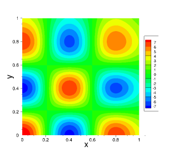
(a) (b)

Figure 1: Poisson equation: (a) Distribution of the exact solution. (b) Distribution of the absolute error of the VarPro solution. In (b), neural network [2, 125, 1], “$\cos$” activation function, $Q=15\times 15$ uniform training collocation points.

We first consider the canonical two-dimensional (2D) Poisson equation on a unit square domain, $(x,y)\in[0,1]\times[0,1]$,

$$\frac{\partial^{2}u}{\partial x^{2}}+\frac{\partial^{2}u}{\partial y^{2}}=f(x,y),$$ (24a)

$$u(x,0)=g_{1}(x),\quad u(x,1)=g_{2}(x),\quad u(0,y)=g_{3}(y),\quad u(1,y)=g_{4}(y),$$ (24b)

where $u(x,y)$ is the field function to be solved for, $f(x,y)$ is a prescribed source term, and $g_{i}$ ($1\leqslant i\leqslant 4$) denote the boundary data. We employ the following analytic solution to this problem in the tests,

$$u=\left[2\cos\left(\frac{3}{2}\pi x+\frac{2}{5}\pi\right)+\frac{3}{2}\cos\left(3\pi x-\frac{\pi}{5}\right)+\frac{1}{1+x^{2}}\right]\left[2\cos\left(\frac{3}{2}\pi y+\frac{2}{5}\pi\right)\right.\\ \left.+\frac{3}{2}\cos\left(3\pi y-\frac{\pi}{5}\right)+\frac{1}{1+y^{2}}\right],$$ (25)

by choosing the source term $f$ and the boundary data $g_{i}$ ($1\leqslant i\leqslant 4$) appropriately. Figure 1(a) shows the distribution of this analytic solution in the $xy$ plane.

We employ feed-forward neural networks with one or two hidden layers, with the architecture given by $[2,M,1]$ or $[2,20,M,1]$, where $M$ is varied systematically or fixed at $M=100$, $125$ or $200$. The two input nodes represent the coordinates $(x,y)$, and the single output node represents the solution field $u(x,y)$. The activation function for the hidden nodes is either the cosine function, $\sigma(x)=\cos(x)$, or the Gaussian function, $\sigma(x)=e^{-x^{2}}$. The output layer is required to be linear (no activation function) and contain no bias.

We employ a uniform set of $Q=Q_{1}\times Q_{1}$ grid points on the domain as the training collocation points, where $Q_{1}$ denotes the number of uniform grid points in each direction (including the two end points) and is varied systematically between around $5$ and $30$ in the tests. After the neural network is trained by the VarPro method on the $Q_{1}\times Q_{1}$ collocation points, the neural network is evaluated on a much larger uniform set of $Q_{2}\times Q_{2}$ grid points, where $Q_{2}=101$ for this problem, to obtain the solution $u(x,y)$. This solution is compared with the analytic solution (25) to compute the maximum ($L^{\infty}$) and the root-mean-squares (rms, or $L^{2}$) errors. These maximum/rms errors are then recorded and referred to as the errors associated with the given neural network architecture and the training collocation points $Q=Q_{1}\times Q_{1}$ for the VarPro method.

parameter	value	parameter	value
neural network	$[2,M,1]$ or $[2,20,M,1]$	training points $Q$	$Q_{1}\times Q_{1}$
$M$	varied	$Q_{1}$	varied
activation function	$\cos$, Gaussian	testing points	$Q_{2}\times Q_{2}$
random seed	$1$	$Q_{2}$	101
initial guess $\bm{\theta}_{0}$	random values on $[-R_{m},R_{m}]$	$R_{m}$	$1.0$
$\delta$ (Algorithm 3)	$0.5$, $1.0$, $2.0$, $5.0$, or $7.0$	$p$ (Algorithm 3)	$0.5$
max-subiterations	$5$	threshold (Algorithm 3)	$1E-12$

Table 1: Poisson equation: Main simulation parameters of the VarPro method.

The main simulation parameters of the VarPro method are summarized in Table 1. The last three rows of this table pertain to the parameters in Algorithm 3. $\bm{\theta}_{0}$ denotes the initial guess to the hidden-layer coefficients in Algorithm 3, which are set to uniform random values generated on $[-R_{m},R_{m}]$ with $R_{m}=1.0$. When comparing the VarPro method and the ELM method, we also employ a value $R_{m}=R_{m0}$ with VarPro, where $R_{m0}$ is the optimal $R_{m}$ value corresponding to ELM computed using the method from DongY2021 . $\delta$ and $p$ in this table are the maximum perturbation magnitude and the preference probability in Algorithm 3, respectively. The “max-subiterations” here refers to the maximum-number-of-sub-iterations in Algorithm 3. The “threshold” here refers to the threshold on the lines $3$ and $19$ in Algorithm 3.

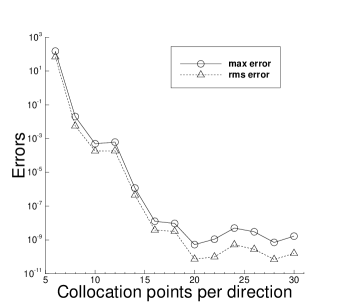
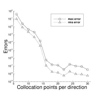
(a) (b)

Figure 2: Poisson equation: Maximum/rms errors of the VarPro solution versus the number of collocation points per direction ($Q_{1}$) obtained with (a) the $\cos$ activation function, and (b) the Gaussian activation function. Neural network [2, 200, 1] in (a,b); $Q_{1}$ is varied in (a,b); $\delta=7.0$ in (a), and $\delta=1.0$ in (b).

Let us first consider the VarPro results obtained with neural networks containing a single hidden layer. Figure 1(b) shows the distribution of the absolute error of the VarPro solution in the $xy$ plane. This result corresponds to the neural network architecture $[2,125,1]$, with the $\cos$ activation function, a uniform set of $Q=15\times 15$ training collocation points, and $\delta=7.0$ in Algorithm 3. The VarPro solution is highly accurate, with a maximum error around $10^{-8}$ in the domain.

Figure 2 illustrates the convergence behavior of the VarPro solution as a function of the number of training collocation points in the domain. Here we employ a neural network $[2,200,1]$, with the $\cos$ and the Gaussian activation functions. The number of collocation points in each direction ($Q_{1}$) is varied systematically. Figure 2 shows the maximum and the rms errors of the VarPro solution in the domain as a function of $Q_{1}$, obtained using the $\cos$ activation function (plot (a)) and the Gaussian activation function (plot (b)). The VarPro errors decrease approximately exponentially when $Q_{1}$ is below around $20$, and then appear to stagnate as $Q_{1}$ further increases. The VarPro errors reach a level around $10^{-11}\sim 10^{-9}$ with the $\cos$ activation function and a level around $10^{-9}\sim 10^{-7}$ with the Gaussian activation function.

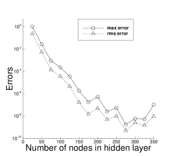
(a) (b)

Figure 3: Poisson equation: The maximum/rms errors of the VarPro solution versus the number of nodes in the hidden layer ($M$), computed using (a) the $\cos$ and (b) the Gaussian activation functions. Neural network [2, $M$, 1], where $M$ is varied in (a,b); $Q=21\times 21$ in (a,b); $\delta=7.0$ in (a) and $\delta=2.0$ in (b).

Figure 3 illustrates the convergence behavior of the VarPro accuracy with respect to the number of nodes in the hidden layer ($M$) of the network. Here we consider neural networks with the architecture $[2,M,1]$, where $M$ is varied systematically, with the $\cos$ and Gaussian activation functions. A fixed uniform set of $Q=21\times 21$ training collocation points is used. Figure 3 shows the maximum/rms errors of the VarPro solution in the domain as a function of $M$, obtained with the $\cos$ (plot(a)) and the Gaussian (plot (b)) activation functions. One can observe an approximately exponential decrease in the VarPro errors with increasing $M$ (when $M$ is below a certain value), and then the errors appear to stagnate (or increase slightly) as $M$ further increases.

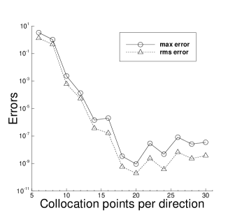
(a) (b)

Figure 4: Poisson equation ($2$ hidden layers in neural network): (a) Error distribution of the VarPro solution. (b) The maximum/rms errors of the VarPro solution versus the number of collocation points per direction ($Q_{1}$). Neural network [2, 20, 100, 1], with the $\cos$ activation function. $Q=18\times 18$ in (a), and is varied in (b). $\delta=0.5$ in (a,b).

Figure 4 illustrates the VarPro solution using a neural network containing two hidden layers. Here we have employed a neural network with the architecture $[2,20,100,1]$ and the $\cos$ activation function for all the hidden nodes. Figure 4(a) shows the distribution of the absolute error of the VarPro solution obtained with a set of $Q=18\times 18$ uniform collocation points in the domain. The maximum error is on the level $10^{-9}$, indicating a high accuracy. Figure 4(b) depicts the maximum/rms errors of the VarPro solution as a function of the number of collocation points in each direction ($Q_{1}$). One can again observe an exponential decrease in the errors (before saturation) with increasing number of collocation points. All these results suggest that the VarPro method produces highly accurate results for solving the Poisson equation.

Neural	$[-R_{m},R_{m}]$	collocation	VarPro		ELM
network		points	max-error	rms-error	max-error	rms-error
[2, 100, 1]	$R_{m}=1$	$5\times 5$	$6.470E+1$	$2.422E+1$	$1.247E+2$	$2.745E+1$
		$10\times 10$	$8.388E-3$	$3.941E-3$	$1.402E+1$	$2.575E+0$
		$15\times 15$	$6.018E-7$	$8.241E-8$	$1.475E+1$	$1.938E+0$
		$20\times 20$	$3.693E-7$	$4.216E-8$	$1.690E+1$	$2.527E+0$
		$25\times 25$	$5.845E-7$	$8.054E-8$	$1.777E+1$	$2.752E+0$
		$30\times 30$	$2.688E-7$	$2.867E-8$	$1.864E+1$	$2.916E+0$
	$R_{m}=R_{m0}$	$5\times 5$	$2.156E+0$	$6.114E-1$	$2.156E+0$	$6.114E-1$
	$\qquad=6$	$10\times 10$	$7.735E-4$	$1.497E-4$	$1.353E-1$	$2.497E-2$
		$15\times 15$	$4.175E-7$	$4.614E-8$	$3.019E-1$	$6.004E-2$
		$20\times 20$	$1.753E-7$	$1.974E-8$	$3.859E-1$	$7.575E-2$
		$25\times 25$	$8.443E-7$	$1.227E-7$	$4.336E-1$	$8.489E-2$
		$30\times 30$	$8.709E-8$	$1.088E-8$	$4.673E-1$	$9.157E-2$
[2, 200, 1]	$R_{m}=1$	$5\times 5$	$5.948E+0$	$2.102E+0$	$9.325E+1$	$2.024E+1$
		$10\times 10$	$2.127E-2$	$4.398E-3$	$4.417E+0$	$7.083E-1$
		$15\times 15$	$6.082E-8$	$1.983E-8$	$5.615E+0$	$8.019E-1$
		$20\times 20$	$1.459E-9$	$1.203E-10$	$4.979E+0$	$7.610E-1$
		$25\times 25$	$1.782E-7$	$7.978E-8$	$5.077E+0$	$8.565E-1$
		$30\times 30$	$3.000E-9$	$3.420E-10$	$5.633E+0$	$8.804E-1$
	$R_{m}=R_{m0}$	$5\times 5$	$7.292E-1$	$2.733E-1$	$7.292E-1$	$2.732E-1$
	$\qquad=6$	$10\times 10$	$1.283E-4$	$3.705E-5$	$1.283E-4$	$3.705E-5$
		$15\times 15$	$2.315E-9$	$4.746E-10$	$9.822E-6$	$7.481E-7$
		$20\times 20$	$3.449E-10$	$3.722E-11$	$1.245E-5$	$1.518E-6$
		$25\times 25$	$6.379E-9$	$4.980E-10$	$1.174E-5$	$1.677E-6$
		$30\times 30$	$4.221E-10$	$4.086E-11$	$1.242E-5$	$1.800E-6$

Table 2: Poisson equation: comparison of the maximum/rms errors obtained using the VarPro and ELM methods. $\cos$ activation function. In both VarPro and ELM, the hidden-layer coefficients are initialized/set to uniform random values generated on $[-R_{m},R_{m}]$, with $R_{m}=1.0$ or with $R_{m}=R_{m0}$. $R_{m0}$ is the optimal $R_{m}$ for ELM computed using the method from DongY2021 , and in this case $R_{m0}=6.0$. $\delta=5.0$ in VarPro.

Table 2 compares the errors of the current VarPro method and the ELM method DongY2021 ; DongL2021 for solving the Poisson equation. We have considered two neural networks having the architecture $[2,M,1]$, with $M=100$ and $M=200$. A uniform set of $Q=Q_{1}\times Q_{1}$ training collocation points are employed on the domain, where $Q_{1}$ is varied between $Q_{1}=5$ and $Q_{1}=30$. In ELM the hidden-layer coefficients are set (and fixed) to uniform random values generated on $[-R_{m},R_{m}]$, and in VarPro the hidden-layer coefficients are initialized (i.e. the initial guess $\bm{\theta}_{0}$ in Algorithm 3) to the same random values from $[-R_{m},R_{m}]$. So the random hidden-layer coefficients in ELM and the initial hidden-layer coefficients in VarPro are identical. We have considered two $R_{m}$ values, $R_{m}=1.0$ and $R_{m}=R_{m0}$, where $R_{m0}$ is the optimal $R_{m}$ for ELM computed using the method from DongY2021 and in this case $R_{m0}=6.0$. We can make the following observations:

• The VarPro method in general produces considerably more accurate results than ELM, under the same settings and conditions, especially when the size of the neural network is still not quite large.

• The ELM accuracy has a fairly strong dependence on the $R_{m}$ value. On the other hand, the VarPro accuracy is less sensitive or insensitive to the $R_{m}$ value.

In these tests the VarPro method has produced errors on the order $10^{-8}\sim 10^{-10}$ with the given neural networks. We should point out that the ELM method can also achieve numerical errors on such levels, but it requires neural networks with a larger number of nodes in the hidden layer.

3.1.2 Advection Equation

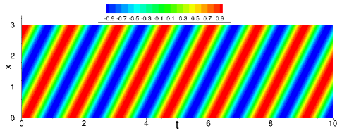
(a) (b)

Figure 5: Advection equation: Distributions of (a) the exact solution, and (b) the absolute error of the VarPro solution, in the spatial-temporal plane. $t_{f}=10$. In (b), $10$ time blocks, $Q=21\times 21$ uniform collocation points per time block, neural network [2, 100, 1], Gaussian activation function, the max sub-iterations is 2 and $\delta=3.0$ in VarPro.

As another linear example we consider the spatial-temporal domain $\Omega=\{(x,t)\ |\ x\in[0,3],\ t\in[0,t_{f}]\}$ in this test, where the temporal dimension $t_{f}$ is to be specified below. We consider the initial/boundary value problem with the advection equation on $\Omega$,

$$\frac{\partial u}{\partial t}-c\frac{\partial u}{\partial x}=0,$$ (26a)

$$u(0,t)=u(3,t),$$ (26b)

$$u(x,0)=\sin\frac{2\pi}{3}(x-2),$$ (26c)

where $u(x,t)$ is the field function to be solved for, and $c=-2.0$ is the wave speed. This problem has the following exact solution,

$$u(x,t)=\sin\frac{2\pi}{3}(x-2t-2).$$ (27)

Figure 5(a) shows the distribution of this exact solution in the spatial-temporal domain with $t_{f}=10$.

To solve this problem with the VarPro method, we employ a feed-forward neural network with one or two hidden layers, with the architecture given by $[2,M,1]$ or $[2,10,M,1]$, where $M$ is varied systematically in the tests. The two input nodes represent the spatial/temporal coordinates $(x,t)$, and the output node represents the solution field $u(x,t)$. We employ the Gaussian function, $\sigma(x)=e^{-x^{2}}$, or the Gaussian error linear unit (GELU) HendrycksG2020 , $\sigma(x)=\frac{1}{2}x\left[1+\text{erf}\left(\frac{x}{\sqrt{2}}\right)\right]$, as the activation function for all the hidden nodes. The output layer is linear and with zero bias.

parameter	value	parameter	value
$t_{f}$	$10$, or $100$	number of time blocks	$10$, or $100$
neural network	$[2,M,1]$, or $[2,10,M,1]$	training points $Q$	$Q_{1}\times Q_{1}$
$M$	varied	$Q_{1}$	varied
activation function	Gaussian, GELU	testing points	$Q_{2}\times Q_{2}$
random seed	$10$	$Q_{2}$	101
initial guess $\bm{\theta}_{0}$	random values on $[-R_{m},R_{m}]$	$R_{m}$	$1.0$
$\delta$ (Algorithm 3)	$0.0$, $0.05$, $1.0$, or $3.0$	$p$ (Algorithm 3)	$0.5$
max-subiterations	$0$, or $2$	threshold (Algorithm 3)	$1E-12$

Table 3: Advection equation: main simulation parameters of the VarPro method.

We primarily consider a temporal dimension $t_{f}=10$ for the domain $\Omega$. We employ the block time marching (BTM) scheme from DongL2021 together with the VarPro method for this problem; see Remark 2.5. We employ $10$ uniform time blocks in time. and in each time block employ a uniform set of $Q=Q_{1}\times Q_{1}$ training collocation points with the VarPro method, where $Q_{1}$ is varied systematically. Following Section 3.1.1, we employ a much larger uniform set of $Q_{2}\times Q_{2}$ grid points within each time block to evaluate the trained neural network for the solution field and compute its errors by comparing with the exact solution (27). We have also considered another spatial-temporal domain with a much larger temporal dimension $t_{f}=100$. Correspondingly, $100$ uniform time blocks are employed in simulations of this case. The main simulation parameters for this problem are summarized in Table 3.

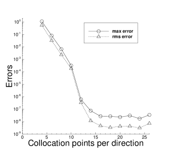
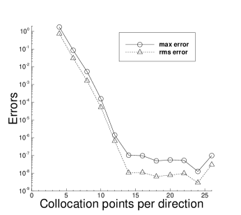
(a) (b)

Figure 6: Advection equation: the maximum/rms errors of the VarPro solution versus the number of collocation points per direction in each time block, obtained with (a) the Gaussian and (b) the GELU activation functions. In (a,b), $t_{f}=10$, $10$ time blocks, neural network $[2,100,1]$, max-subiterations = 2 and $\delta=1.0$ in VarPro.

Let us first look into the VarPro errors obtained using neural networks with one hidden layer. Figure 5(b) shows the distribution of the absolute error of the VarPro result in the spatial-temporal domain. This result is for the temporal dimension $t_{f}=10$, and is obtained using a neural network $[2,100,1]$ with the Gaussian activation function and a uniform set of $Q=21\times 21$ training collocation points in the domain. The VarPro result is highly accurate, with a maximum error on the order $10^{-8}$ in the overall domain.

Figure 6 illustrates the convergence behavior of the VarPro solution with respect to the number of collocation points per direction ($Q_{1}$) in each time block. This is for the temporal dimension $t_{f}=10$ computed with a neural network $[2,100,1]$ and $10$ time blocks . The plot (a) shows the maximum and rms errors in the overall domain of the VarPro solution as a function of $Q_{1}$ obtained with the Gaussian activation function. The plot (b) shows the corresponding result obtained with the GELU activation function. The exponential decrease in the errors with increasing number of collocation points (before saturation) is unmistakable.

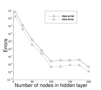
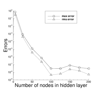
(a) (b)

Figure 7: Advection equation: the maximum/rms errors of the VarPro solution versus the number of nodes in the hidden layer ($M$) obtained with (a) the Gaussian and (b) the GELU activation functions. In (a,b), $t_{f}=10$, $10$ time blocks, $Q=21\times 21$ uniform collocation points, neural network $[2,M,1]$ with $M$ varied, max-subiterations$=2$ and $\delta=1.0$ in VarPro.

Figure 7 illustrates the convergence behavior of the VarPro solution with respect to the number of nodes in the hidden layer ($M$). Here the domain corresponds to $t_{f}=10$, with $10$ time blocks and a uniform set of $Q=21\times 21$ training collocation points per time block in the VarPro simulation. The neural network is given by $[2,M,1]$, where $M$ is varied systematically. Figures 7(a) and (b) shows the maximum/rms errors in the overall domain as a function of $M$ obtained using the Gaussian and the GELU activation functions, respectively. The exponential decrease in the errors with increasing $M$ (before saturation) is evident.

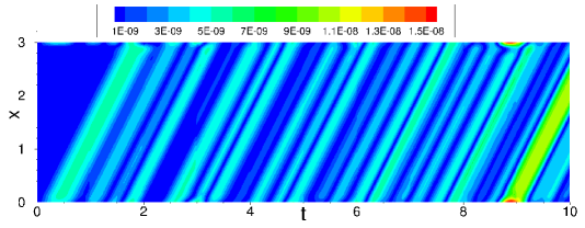
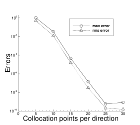
(a) (b)

Figure 8: Advection equation (two hidden layers in NN): (a) Error distribution of the VarPro solution in the spatial-temporal plane, and (b) the maximum/rms errors of the VarPro solution versus the number of collocation points per direction, obtained with $2$ hidden layers in the neural network. In (a,b), $t_{f}=10$, $10$ uniform time blocks, neural network $[2,10,100,1]$, Gaussian activation function, max-subiterations = 2 and $\delta=0.05$ in VarPro. $Q=21\times 21$ in (a) and is varied in (b).

Figure 8 illustrates the VarPro results computed using a neural network containing two hidden layers. The domain corresponds to $t_{f}=10$, and the neural network has the architecture $[2,10,100,1]$ with the Gaussian activation function. Figure 8(a) shows the VarPro error distribution in the overall spatial-temporal plane, obtained with a uniform $Q=21\times 21$ training collocation points per time block. Figure 8(b) depicts the maximum/rms VarPro errors in the overall domain as a function of the collocation points per direction in each time block, demonstrating the exponential convergence behavior.

$[-R_{m},R_{m}]$	collocation	VarPro		ELM
	points	max-error	rms-error	max-error	rms-error
$R_{m}=1$	$5\times 5$	$2.505E-1$	$1.005E-1$	$2.505E-1$	$1.005E-1$
	$10\times 10$	$3.194E-4$	$1.864E-4$	$3.758E-4$	$1.245E-4$
	$15\times 15$	$4.254E-8$	$6.954E-9$	$4.232E-5$	$1.269E-5$
	$20\times 20$	$2.348E-8$	$4.240E-9$	$4.618E-5$	$1.402E-5$
	$25\times 25$	$1.493E-8$	$2.889E-9$	$5.471E-5$	$1.598E-5$
	$30\times 30$	$1.354E-8$	$2.528E-9$	$6.419E-5$	$1.773E-5$
$R_{m}=R_{m0}$	$5\times 5$	$1.038E-1$	$3.252E-2$	$1.038E-1$	$3.252E-2$
$\qquad=0.7$	$10\times 10$	$1.996E-4$	$9.437E-5$	$2.240E-4$	$6.519E-5$
	$15\times 15$	$7.934E-8$	$9.495E-9$	$3.881E-5$	$9.642E-6$
	$20\times 20$	$9.261E-8$	$3.253E-8$	$3.471E-5$	$1.060E-5$
	$25\times 25$	$3.444E-8$	$4.931E-9$	$3.314E-5$	$1.117E-5$
	$30\times 30$	$4.670E-8$	$7.428E-9$	$3.283E-5$	$1.164E-5$

Table 4: Advection equation: comparison of the maximum/rms errors of the solutions obtained using the VarPro and ELM methods. $t_{f}=10$, $10$ time blocks, Neural network [2, 100, 1], Gaussian activation function. In VarPro, the max-subiterations is 2 and $\delta=1.0$. In ELM/VarPro, the hidden-layer coefficients are set/initialized to uniform random values from $[-R_{m},R_{m}]$, with $R_{m}=1.0$ or with $R_{m}=R_{m0}=0.7$.

A comparison between the current VarPro method and the ELM method DongY2021 ; DongL2021 for solving the advection equation is provided in Table 4. The maximum and rms errors of the VarPro and the ELM methods obtained on a series of training collocation points are listed. These results are for the domain $t_{f}=10$, with $10$ time blocks in block time marching. We have employed a neural network $[2,100,1]$ with the Gaussian activation function. The random hidden-layer coefficients in ELM and the initial hidden-layer coefficients in VarPro are generated by $R_{m}=1$ and $R_{m}=R_{m0}=0.7$. It is evident that VarPro generally leads to significantly more accurate results than ELM.

(a) (b)

Figure 9: Advection equation (long-time simulation): Distributions of (a) the VarPro solution and (b) its absolute error in the spatial-temporal domain. Domain: $(x,t)\in[0,3]\times[0,100]$, 100 uniform time blocks, $Q=25\times 25$ uniform collocation points per time block, neural network $[2,150,1]$, Gaussian activation function, no subiteration (max-subiterations=0) in VarPro.

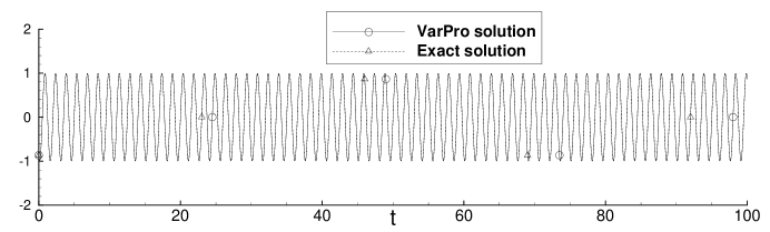
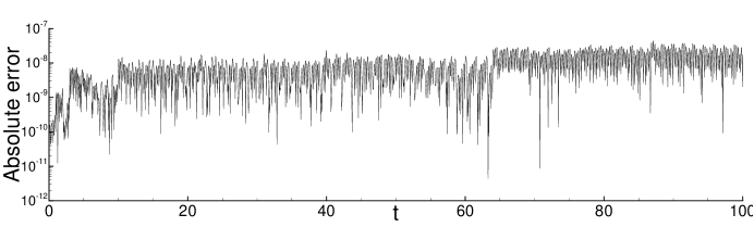
(a) (b)

Figure 10: Advection equation (long-time simulation): (a) Comparison of the time histories between the VarPro solution and the exact solution at the mid-point of the domain ($x=1.5$). (b) Time history of the absolute error of the VarPro solution at the mid-point of the domain ($x=1.5$). Simulation parameters and configurations here follow those of Figure 9.

Figures 9 and 10 illustrate a longer-time simulation of the advection equation using the VarPro method and the block time marching scheme. Here the domain corresponds to $t_{f}=100$. We have employed $100$ uniform time blocks, a set of $Q=25\times 25$ uniform collocation points per time time block, and a neural network $[2,150,1]$ with the Gaussian activation function. Figures 9(a) and (b) show the distributions of the VarPro solution and its absolute errors in the overall spatial-temporal plane. It can be observed that the VarPro method has produced highly accurate results, with the maximum error on the order $10^{-8}$ in this long-time simulation. Figure 10(a) compares the time histories of the VarPro solution and the exact solution (27) at the mid-point of the domain ($x=1.5$), and Figure 10(b) shows the corresponding VarPro error history at this point. These results indicate that the VarPro method together with the block time marching scheme can produce highly accurate results in long-time simulations.

3.2 Nonlinear Examples

3.2.1 Nonlinear Helmholtz Equation

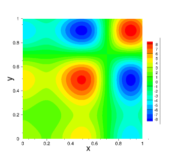
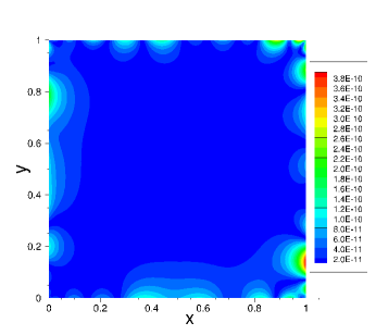
(a) (b)

Figure 11: Nonlinear Helmholtz equation: Distributions of (a) the exact solution and (b) the absolute error of the VarPro solution. In (b), neural network [2, 200, 1], “$\sin$” activation function, $Q=21\times 21$ uniform collocation points, $\delta=0.05$ in VarPro.

In the first nonlinear example, we consider the boundary value problem with a nonlinear Helmholtz equation on the unit square domain $[0,1]\times[0,1]$,

$$\frac{\partial^{2}u}{\partial x^{2}}+\frac{\partial^{2}u}{\partial y^{2}}-100u+5\cos(2u)=f(x,y),$$ (28a)

$$u(x,0)=g_{1}(x),\quad u(x,1)=g_{2}(x),\quad u(0,y)=g_{3}(y),\quad u(1,y)=g_{4}(y),$$ (28b)

where $u(x,y)$ is the field function to be solved for, $f(x,y)$ is a prescribed source term, and $g_{i}$ ($1\leqslant i\leqslant 4$) denote the boundary data. With $f$ and $g_{i}$ ($1\leqslant i\leqslant 4$) chosen appropriately, this problem admits the following analytic solution,

$$u=\left[\frac{5}{2}\cos\left(\frac{3}{2}\pi x-\frac{2}{5}\pi\right)+\frac{3}{2}\cos\left(3\pi x+\frac{3\pi}{10}\right)+\frac{1}{2}(e^{x}-e^{-x})\right]\left[\frac{5}{2}\cos\left(\frac{3}{2}\pi y-\frac{2}{5}\pi\right)\right.\\ \left.+\frac{3}{2}\cos\left(3\pi y+\frac{3\pi}{10}\right)+\frac{1}{2}(e^{y}-e^{-y})\right].$$ (29)

We employ this analytic solution in the following tests. Figure 11(a) shows the distribution of this analytic solution in the $xy$ plane.

parameter	value	parameter	value
neural network	$[2,M,1]$, or $[2,5,M,1]$	training points $Q$	$Q_{1}\times Q_{1}$
$M$	varied	$Q_{1}$	varied
activation function	$\sin$, Gaussian	testing points	$Q_{2}\times Q_{2}$
random seed	$1$	$Q_{2}$	101
initial guess $\bm{\theta}_{0}$	random values on $[-R_{m},R_{m}]$	$R_{m}$	$1.0$
$\delta$ (Algorithm 3)	$0.02$, $0.05$, $0.1$, or $0.2$	$p$ (Algorithm 3)	$0.5$
max-subiterations	$2$	threshold (Algorithm 3)	$1E-12$
max-iterations-newton	$20$	tolerance-newton	$1E-8$

Table 5: Nonlinear Helmholtz equation: main simulation parameters of the VarPro method.

We employ neural networks with the architectures $[2,M,1]$ and $[2,5,M,1]$ in the VarPro simulations, where $M$ is varied in the tests. The sine function, $\sigma(x)=\sin(x)$, or the Gaussian function, $\sigma(x)=e^{-x^{2}}$, is employed as the activation functions for the hidden nodes. A uniform set of $Q=Q_{1}\times Q_{1}$ training collocation points, where $Q_{1}$ is varied, is used to train the neural network. The VarPro solution is computed on a larger set of $Q_{2}\times Q_{2}$ (with $Q_{2}=101$) uniform grid points by evaluating the trained neural network, and compared with the analytic solution to compute its errors. Table 5 provides the main simulation parameters for this problem and the VarPro method. In this table “max-iterations-newton” denotes the maximum number of Newton iterations, and “tolerance-newton” denotes the relative tolerance for the Newton iteration (see lines $3$ and $9$ of Algorithm 4).

Figure 11(b) illustrates the error distribution of a VarPro solution in the $xy$ plane, computed using a neural network $[2,200,1]$ with the $\sin$ activation function and a uniform set of $Q=21\times 21$ collocation points. The result is observed to be highly accurate, with a maximum error on the order $10^{-10}$ in the domain.

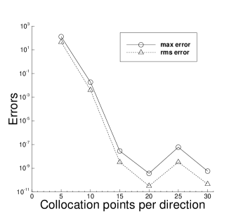
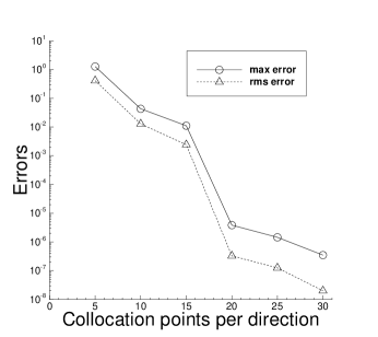
(a) (b)

Figure 12: Nonlinear Helmholtz equation: the maximum/rms errors of the VarPro solution versus the number of collocation points per direction, obtained using (a) the sine and (b) the Gaussian activation functions. Neural network [2, 200, 1], $\delta=0.1$ in (a) and $\delta=0.2$ in (b) with VarPro.

Figure 12 illustrates the convergence behavior of the VarPro method with respect to the number of training collocation points in the domain. In these tests the number of collocation points per direction ($Q_{1}$) is varied systematically. The two plots show the maximum/rms errors in the domain of the VarPro solution as a function of $Q_{1}$, obtained using the $\sin$ (plot (a)) and the Gaussian (plot (b)) activation functions. These VarPro results are attained using a neural network $[2,200,1]$. We observe an exponential decrease in the VarPro errors (before saturation) with increasing number of collocation points.

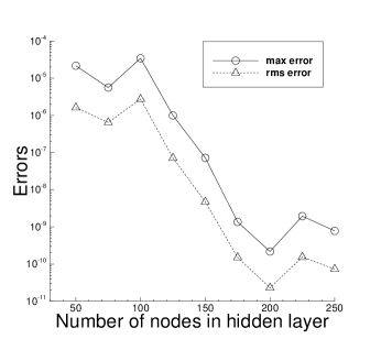
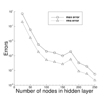
(a) (b)

Figure 13: Nonlinear Helmholtz equation: the maximum/rms errors of the VarPro solution versus the number of nodes in the hidden layer, obtained with (a) the sine and (b) the Gaussian activation functions. Neural network $[2,M,1]$, where $M$ is varied, $Q=21\times 21$, $\delta=0.1$ in (a) and $\delta=0.2$ in (b) with VarPro.

Figure 13 illustrates the convergence behavior of the VarPro solution with respect to the number of nodes in the hidden layer ($M$) for the nonlinear Helmholtz equation. Here the neural network has an architecture $[2,M,1]$, where $M$ is varied systematically, and a uniform set of $Q=21\times 21$ training collocation points is employed in the simulation. This figure shows the maximum/rms errors in the domain as a function of $M$, obtained using the sin (plot (a)) and the Gaussian (plot (b)) activation functions. The errors computed with the $\sin$ activation function appear not quite regular as $M$ increases. But overall all these errors appear to decrease approximately exponentially with increasing $M$.

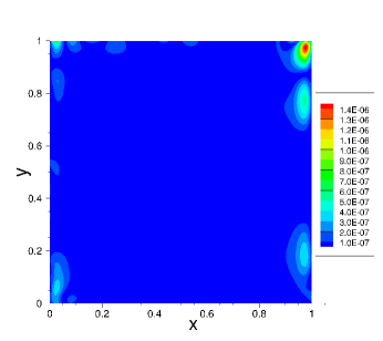
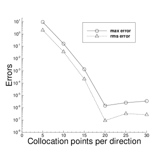
(a) (b)

Figure 14: Nonlinear Helmholtz equation (two hidden layers in NN): (a) Error distribution of the VarPro solution. (b) The VarPro maximum/rms errors versus the number of collocation points per direction ($Q_{1}$). Neural network [2, 5, 200, 1], $\sin$ activation function, $Q=20\times 20$ in (a) and is varied in (b), $\delta=0.02$ in (a,b) with VarPro.

Figure 14 illustrates the VarPro results obtained using two hidden layers in the neural network. Here we consider a neural network with the architecture $[2,5,200,1]$, with the $\sin$ activation function. Figure 14(a) shows the error distribution of the VarPro solution obtained using $Q=20\times 20$ training collocation points. In Figure 14(b) the number of collocation points per direction ($Q_{1}$) is varied systematically, and the maximum/rms errors are plotted as a function of $Q_{1}$. An exponential decrease in the errors (before saturation) can be observed.

$[-R_{m},R_{m}]$	collocation	VarPro		ELM
	points	max-error	rms-error	max-error	rms-error
$R_{m}=1$	$5\times 5$	$1.297E+2$	$4.536E+1$	$4.388E+0$	$8.195E-1$
	$10\times 10$	$1.855E-2$	$3.955E-3$	$7.701E+0$	$1.210E+0$
	$15\times 15$	$2.868E-8$	$3.252E-9$	$3.743E-1$	$4.767E-2$
	$20\times 20$	$3.679E-10$	$3.203E-11$	$1.280E+0$	$1.864E-1$
	$25\times 25$	$6.014E-8$	$3.281E-9$	$1.434E+0$	$2.198E-1$
	$30\times 30$	$5.709E-10$	$4.576E-11$	$8.365E-1$	$1.123E-1$
$R_{m}=R_{m0}=4.4$	$5\times 5$	$6.742E-1$	$2.408E-1$	$1.182E-1$	$3.589E-2$
	$10\times 10$	$5.869E-3$	$1.169E-3$	$8.987E-7$	$1.861E-7$
	$15\times 15$	$7.130E-9$	$1.024E-9$	$6.690E-9$	$8.655E-10$
	$20\times 20$	$2.851E-9$	$2.364E-10$	$2.384E-8$	$2.835E-9$
	$25\times 25$	$4.193E-10$	$5.173E-11$	$3.133E-8$	$3.611E-9$
	$30\times 30$	$1.128E-9$	$1.029E-10$	$3.813E-8$	$4.194E-9$

Table 6: Nonlinear Helmholtz equation: comparison of the maximum/rms errors of the VarPro and ELM solutions. Neural network [2, 200, 1], $\sin$ activation function. In VarPro, $\delta=0.1$, and the tolerance-newton is set to $1E-8$ with $R_{m}=1$ and to $1E-14$ with $R_{m}=4.4$.

Table 6 is a comparison of the errors between the VarPro method and the ELM method for solving the nonlinear Helmholtz equation. These results are for a neural network $[2,200,1]$ with the $\sin$ activation function. In ELM the random hidden-layer coefficients are set to, and in VarPro the hidden-layer coefficients are initialized to, uniform random values from $[-R_{m},R_{m}]$, where $R_{m}=1.0$ or $R_{m}=R_{m0}=4.4$. Several sets of uniform training collocation points are tested, ranging from $Q=5\times 5$ to $Q=30\times 30$. The VarPro results are in general markedly more accurate than those of the ELM results. This is especially pronounced for those cases corresponding to $R_{m}=1.0$.

3.2.2 Viscous Burgers’ Equation

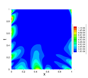
(a) (b)

Figure 15: Burgers’ equation: Distributions of (a) the exact solution and (b) the absolute error of the VarPro solution in the spatial-temporal plane. In (b), neural network [2, 150, 1], and $Q=31\times 31$ training collocation points.

In the second nonlinear example we use the viscous Burgers’ equation to test the VarPro method. Consider the spatial-temporal domain, $Q=\{(x,t)\ |\ x\in[0,1],\ t\in[0,1]\}$, and the following initial/boundary value problem on $\Omega$,

$$\frac{\partial u}{\partial t}+u\frac{\partial u}{\partial x}-\nu\frac{\partial^{2}u}{\partial x^{2}}=f(x,t),$$ (30a)

$$u(0,t)=g_{1}(t),\quad u(1,t)=g_{2}(t),$$ (30b)

$$u(x,0)=h(x).$$ (30c)

In the above equations, $u(x,t)$ is the field function to be solved for, $\nu=0.05$, $f(x,t)$ is a prescribed source term, $g_{1}$ and $g_{2}$ are the boundary conditions, and $h$ is the initial condition. We choose $f$, $g_{1}$, $g_{2}$ and $h$ such that this problem has the the following analytic solution,

$$u(x,t)=\left[2\cos\left(\pi x+\frac{2\pi}{5}\right)+\frac{3}{2}\cos\left(2\pi x-\frac{3\pi}{5}\right)\right]\left[2\cos\left(\pi t+\frac{2\pi}{5}\right)+\frac{3}{2}\cos\left(2\pi t-\frac{3\pi}{5}\right)\right].$$ (31)

Figure 15(a) shows the distribution of this analytic solution in the spatial-temporal plane.

parameter	value	parameter	value
domain	$(x,t)\in[0,1]\times[0,1]$	block time marching	none
neural network	$[2,M,1]$	training points $Q$	$Q_{1}\times Q_{1}$
$M$	varied	$Q_{1}$	varied
activation function	Gaussian	testing points	$Q_{2}\times Q_{2}$
random seed	$10$	$Q_{2}$	101
initial guess $\bm{\theta}_{0}$	random values on $[-R_{m},R_{m}]$	$R_{m}$	$1.0$
$\delta$ (Algorithm 3)	un-used	$p$ (Algorithm 3)	un-used
max-subiterations	$0$ (no subiteration)	threshold (Algorithm 3)	$1E-12$
max-iterations-newton	$50$	tolerance-newton	$1E-8$

Table 7: Burgers’ equation: main simulation parameters of the VarPro method.

We employ neural networks with an architecture $[2,M,1]$ in the VarPro simulations, where $M$ is varied systematically in the tests. The two input nodes represent $(x,t)$ and the linear output node represents the solution field $u(x,t)$. The Gaussian activation function, $\sigma(x)=e^{-x^{2}}$, is employed in all the hidden nodes. A uniform set of $Q=Q_{1}\times Q_{1}$ collocation points in the spatial-temporal domain is used to train the neural network with the VarPro method, and $Q_{1}$ is varied systematically in the tests. The trained neural network is evaluated on a larger set of $Q_{2}\times Q_{2}$ uniform grid points to attain the field solution, which is then compared with the analytic solution (31) to compute the errors. The main simulation parameters for this problem are summarized in Table 7.

Figure 15(b) illustrates the distribution of the absolute error of a VarPro solution in the spatial-temporal plane. This is computed using a neural network $[2,150,1]$ with a uniform set of $Q=31\times 31$ training collocation points. The VarPro solution can be observed to be quite accurate, with a maximum error on the order $10^{-8}$ in the domain.

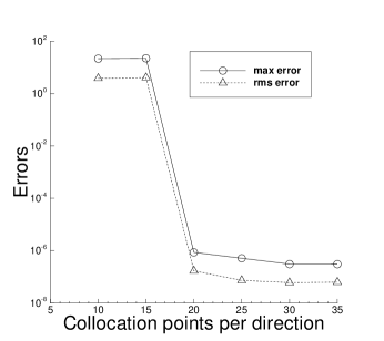
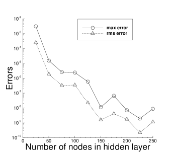
(a) (b)

Figure 16: Burgers’ equation: The maximum/rms errors of the VarPro solution versus (a) the number of collocation points in each direction ($Q_{1}$), and (b) the number of nodes in the hidden layer ($M$) of the neural network. Neural network $[2,M,1]$, $Q=Q_{1}\times Q_{1}$ uniform collocation points. $M=100$ in (a) and is varied in (b). $Q_{1}=31$ in (b) and is varied in (a).

Figure 16 illustrates the convergence behavior of the VarPro method for solving the Burgers’ equation. In these tests the neural network is given by $[2,M,1]$, where $M$ is either fixed at $M=100$ or varied between $M=25$ and $M=250$. A set of $Q=Q_{1}\times Q_{1}$ uniform training collocation points is used, where $Q_{1}$ is either fixed at $Q_{1}=31$ or varied between $Q_{1}=10$ and $Q_{1}=35$. Figure 16(a) shows the maximum/rms errors of the VarPro solution as a function of $Q_{1}$, corresponding to a fixed $M=100$ for the neural network. The error behavior is not quite regular. With a smaller $Q_{1}$ (e.g. $10$ or $15$) the errors are at a level $1\sim 10$, while with a larger $Q_{1}$ ($20$ and beyond) the errors abruptly drop to a level around $10^{-8}\sim 10^{-6}$. We observe that with the smaller $Q_{1}=10$ and $15$ the Newton iteration fails to converge to the prescribed tolerance within the prescribed maximum number of iterations. Figure 16(b) shows the maximum/rms errors as a function of $M$, corresponding to a fixed $Q=31\times 31$ for the collocation points. The errors can be observed to decrease approximately exponentially with increasing $M$.

$[-R_{m},R_{m}]$	$M$	VarPro		ELM
		max-error	rms-error	max-error	rms-error
$R_{m}=1$	$25$	$3.111E-3$	$2.499E-4$	$6.382E+0$	$8.382E-1$
	$50$	$1.538E-5$	$1.890E-6$	$6.669E-2$	$1.016E-2$
	$75$	$2.603E-6$	$3.222E-7$	$1.216E-2$	$1.406E-3$
	$100$	$2.406E-6$	$3.471E-7$	$4.189E-4$	$6.540E-5$
	$125$	$5.894E-7$	$2.193E-8$	$1.088E-4$	$1.099E-5$
	$150$	$1.131E-8$	$1.599E-9$	$4.387E-6$	$5.623E-7$
$R_{m}=R_{m0}=0.9$	$25$	$1.592E-3$	$2.150E-4$	$3.501E+0$	$6.245E-1$
	$50$	$1.069E-5$	$1.794E-6$	$1.390E-1$	$7.607E-3$
	$75$	$3.049E-6$	$3.576E-7$	$1.948E-2$	$1.524E-3$
	$100$	$4.831E-6$	$3.311E-7$	$7.639E-4$	$4.780E-5$
	$125$	$4.163E-7$	$7.029E-8$	$5.864E-5$	$6.823E-6$
	$150$	$6.063E-8$	$7.242E-9$	$2.000E-6$	$2.877E-7$

Table 8: Burgers’ equation: comparison of the maximum/rms errors of the VarPro and ELM solutions. Neural network $[2,M,1]$ with $M$ varied; fixed $Q=31\times 31$ training collocation points.

Table 8 provides a comparison of the solution errors obtained using the VarPro method and the ELM method DongY2021 ; DongL2021 for the Burgers’ equation. These are computed using a fixed uniform set of $Q=31\times 31$ collocation points and a series of neural networks with the architecture $[2,M,1]$, where $M$ is varied between $M=25$ and $M=150$. The random hidden-layer coefficients in ELM are set, and the hidden-layer coefficients in VarPro are initialized, by using $R_{m}=1$ and $R_{m}=R_{m0}=0.9$ in the tests. It is evident that the VarPro method produces significantly more accurate results than the ELM method.

3.2.3 Nonlinear Klein-Gordon Equation

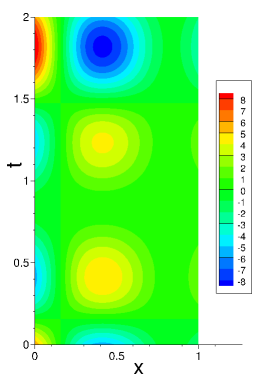
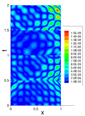
(a) (b)

Figure 17: Nonlinear Klein-Gordon equation: Distributions of (a) the exact solution and (b) the absolute error of the VarPro solution in the spatial-temporal plane. In (b), $4$ uniform time blocks in domain, neural network $[2,200,1]$, $Q=21\times 21$ uniform collocation points per time block.

In the last example we use the nonlinear Klein-Gordon equation Strauss1978 to test the VarPro method. Consider the spatial-temporal domain, $\Omega=\{(x,t)\ |\ x\in[0,1],\ t\in[0,2]\}$, and the initial/boundary value problem with the nonlinear Klein-Gordon equation on $\Omega$,

$$\frac{\partial^{2}u}{\partial t^{2}}-\frac{\partial^{2}u}{\partial x^{2}}+u+\sin(u)=f(x,t),$$ (32a)

$$u(0,t)=g_{1}(t),\quad u(1,t)=g_{2}(t),$$ (32b)

$$u(x,0)=h_{1}(x),\quad\left.\frac{\partial u}{\partial t}\right|_{(x,0)}=h_{2}(x),$$ (32c)

where $u(x,t)$ is the field function to be solved for, $f(x,t)$ is a prescribed source term, $g_{1}$ and $g_{2}$ are the boundary conditions, and $h_{1}$ and $h_{2}$ are the initial conditions. We choose the source term, the boundary and initial conditions appropriately such that this problem has the following analytic solution,

$$u(x,t)=\left[2\cos\left(\pi x+\frac{\pi}{5}\right)+\frac{9}{5}\cos\left(2\pi x+\frac{7\pi}{20}\right)\right]\left[2\cos\left(\pi t+\frac{\pi}{5}\right)+\frac{9}{5}\cos\left(2\pi t+\frac{7\pi}{20}\right)\right].$$ (33)

We employ this analytic solution to test the accuracy of the VarPro method. Figure 17(a) shows the distribution of this analytic solution in the spatial-temporal plane.

parameter	value	parameter	value
domain	$(x,t)\in[0,1]\times[0,2]$	time blocks	$4$
neural network	$[2,M,1]$	training points $Q$	$Q_{1}\times Q_{1}$
$M$	varied	$Q_{1}$	varied
activation function	Gaussian	testing points	$Q_{2}\times Q_{2}$
random seed	$22$	$Q_{2}$	101
initial guess $\bm{\theta}_{0}$	random values on $[-R_{m},R_{m}]$	$R_{m}$	$1.0$
$\delta$ (Algorithm 3)	un-used	$p$ (Algorithm 3)	un-used
max-subiterations	$0$ (no subiteration)	threshold (Algorithm 3)	$1E-12$
max-iterations-newton	$20$	tolerance-newton	$1E-8$

Table 9: Nonlinear Klein-Gordon equation: main simulation parameters of the VarPro method.

We employ the block time marching scheme DongL2021 together with the VarPro method to solve this problem. We use $4$ uniform time blocks in the domain, and on each time block employ a neural network with the architecture $[2,M,1]$, where $M$ is varied in the tests. The two input nodes represent $(x,t)$, and the linear output node represents the field solution $u(x,t)$. The Gaussian activation function $\sigma(x)=e^{-x^{2}}$ is employed for all the hidden nodes. On each time block a uniform set of $Q=Q_{1}\times Q_{1}$ collocation points, where $Q_{1}$ is varied, is used to train the neural network. The trained neural network is evaluated on a larger set of $Q_{2}\times Q_{2}$ uniform grid points to obtain the field solution $u(x,t)$, which is compared with the exact solution (33) to compute the errors of the VarPro simulation. Table 9 summarizes the main simulation parameters for this problem.

Figure 17(b) shows the distribution of the absolute error of a VarPro simulation in the spatial-temporal plane. In this simulation the neural network architecture is given by $[2,200,1]$, and a uniform set of $Q=21\times 21$ training collocation points is used on each time block. The maximum error level is around $10^{-8}$ on the overall domain, indicating that the VarPro result is quite accurate.

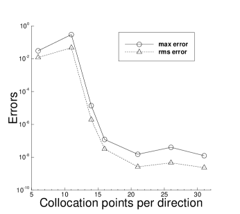
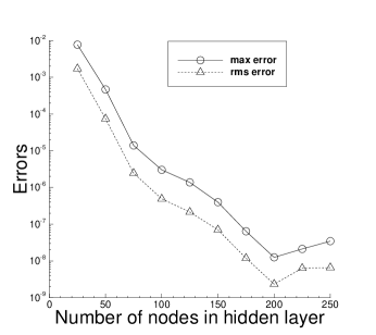
(a) (b)

Figure 18: Nonlinear Klein-Gordon equation: the maximum/rms errors of the VarPro solution in the overall domain versus (a) the number of collocation points per direction ($Q_{1}$) in each time block, and (b) the number of nodes in the hidden layer ($M$) of the neural network. In (a,b), neural network $[2,M,1]$, with $Q=Q_{1}\times Q_{1}$ training collocation points. $M=200$ in (a) and is varied in (b). $Q_{1}=31$ in (b) and is varied in (a).

Figure 18 illustrates the convergence behavior of the VarPro method for solving the nonlinear Klein-Gordon equation. Here we employ the neural network $[2,M,1]$, and $Q=Q_{1}\times Q_{1}$ uniform collocation points in each time block. In the first group of tests we fix $M=200$ and vary $Q_{1}$ systematically. In the second group of tests we fix $Q_{1}=31$ and vary $M$ systematically. The maximum and rms errors of the VarPro solution in the overall domain are computed for each case. Figure 18(a) shows these errors as a function of $Q_{1}$ for the first group of tests, and Figure 18(b) shows these errors as a function of $M$ for the second group of tests. These results indicate that the VarPro errors decrease approximately exponentially with increasing number of collocation points or with increasing number of nodes in the hidden layer. We also notice some irregularity in the errors of Figure 18(a) when the number of collocation points is small.

4 Concluding Remarks

In this paper we have presented a variable projection-based method together with artificial neural networks for numerically approximating linear and nonlinear partial differential equations. The basic idea of variable projection (VarPro) for solving separable nonlinear least squares problems is to distinguish the linear parameters from the nonlinear parameters, and then eliminate the linear parameters to attain a reduced formulation of the problem. One can then solve the reduced problem for the nonlinear parameters first, and then compute the linear parameters by using the linear least squares method afterwards.

Approximating linear PDEs (with linear boundary/initial conditions) by variable projection and artificial neural networks is conceptually straightforward. In this case, in the resultant nonlinear least squares problem the coefficients in the linear output layer are the linear parameters, and those in the hidden layers are the nonlinear parameters. The output-layer coefficients can be expressed in terms of the hidden-layer coefficients by solving a linear least squares problem, and they can be eliminated from the problem. The reduced problem involves only the hidden-layer coefficients, and it can be solved by the nonlinear least squares method. The main issues with the VarPro implementation lie in the computations of the residual function and the Jacobian matrix of the reduced problem. We have discussed in some detail how to implement these computations with neural networks in Algorithms 1 and 2 and in the Remarks 2.1 and 2.2.

For approximating nonlinear PDEs, or linear PDEs with nonlinear boundary/initial conditions, the variable projection approach with the artificial neural networks cannot be directly used. This is because the resultant nonlinear least squares problem is not separable. In this case, all the weight/bias coefficients in the neural network become nonlinear parameters, even if the output layer contains no activation function.

To overcome this issue, we have presented a Newton/variable projection (Newton-VarPro) method for approximating nonlinear PDEs, or linear PDEs with nonlinear boundary/initial conditions. We first linearize the problem, with a particular linearized form for the Newton iteration. The linearization is formulated in terms of the updated approximation field, not the increment field. This linearization is critical to the accuracy of the current Newton-VarPro method. The linearized system can be solved by the variable projection approach together with artificial neural networks. Therefore for solving nonlinear PDEs, our method involves an overall Newton iteration, and within each iteration the variable projection method is used to solve the linearized problem to attain the updated approximation field. Upon convergence of the Newton iteration, the solution to the nonlinear problem is represented by the weight/bias coefficients of the neural network.

We have presented ample numerical examples with linear and nonlinear PDEs to test the accuracy of the variable projection method. It is observed that, for smooth field solutions, the errors of the VarPro method decrease exponentially or nearly exponentially with increasing number of collocation points or with increasing number of output-layer coefficients. The test results unequivocally show that the VarPro method is highly accurate. Even with a fairly small number of nodes in the neural network, or with a fairly small set of collocation points, the VarPro method can produce very accurate simulation results.

In particular, we have compared extensively the current VarPro method with the extreme learning machine (ELM) method DongY2021 , which is arguably the most accurate neural network-based PDE solver so far DongL2021 ; DongY2021 . Under the same simulation conditions and settings, the VarPro method generally leads to significantly more accurate results than the ELM method, especially in cases with a fairly small or a moderate number of nodes in the neural network.

Test problem	neural	collocation	VarPro training	ELM training
	network	points	time (seconds)	time (seconds)
Advection equation	$[2,100,1]$	$10\times 10$	$7.4$	$0.29$
		$15\times 15$	$15.4$	$0.31$
		$20\times 20$	$78.2$	$0.32$
Nonlinear Helmholtz	$[2,200,1]$	$10\times 10$	$1.7$	$2.0$
equation		$15\times 15$	$36.5$	$2.8$
		$20\times 20$	$78.1$	$4.0$

Table 10: Comparison of the computational cost (network training time) between VarPro and ELM for solving the advection equation (Section 3.1.2) and the nonlinear Helmholtz equation (Section 3.2.1). The hidden-layer coefficients in ELM are set/fixed to, and the hidden-layer coefficients in VarPro are initialized to, uniform random values from $[-R_{m},R_{m}]$ with $R_{m}=1.0$. The cases in this table are selected from and correspond to those cases in Tables 4 and 6. Please refer to the corresponding cases in Tables 4 and 6 for the VarPro/ELM errors.

While the VarPro method is significantly superior to ELM in terms of the accuracy, its computational cost (i.e. training time of the neural network) is generally much higher than that of the ELM method. This is because in VarPro one needs to solve the reduced problem for the hidden-layer coefficients by a nonlinear least squares computation, apart from the computation for the linear output-layer coefficients. In contrast, in ELM only the linear output-layer coefficients are computed, while the hidden-layer coefficients in the neural network are fixed to the random values that are pre-set. Table 10 illustrates this points with a list of the network training time for the VarPro method and the ELM method with selected cases in solving the the advection equation (Section 3.1.2) and the nonlinear Helmholtz equation (Section 3.2.1).

The variable projection method is a powerful technique for training artificial neural networks, providing a considerably superior accuracy for scientific machine learning, as demonstrated by ample numerical examples in the current paper. The Newton-VarPro method developed herein provides an effective tool and enables the use of the variable projection strategy to tackle nonlinear problems in scientific machine learning. The application potential of this technique is enormous. This and related aspects, as well as further studies and improvements, of this technique will be pursued in a future endeavor.

References

- [1] A.Y. Aravkin and T. van Leeuwen. Estimating nuisance parameters in inverse problems. Inverse Problems, 28:115016, 2012.
- [2] T. Askham and J.N. Kutz. Variable projection methods for an optimized dynamic mode decomposition. SIAM J. Applied Dynamical Systems, 17:380–416, 2018.
- [3] A. Bjorck. Numerical Methods in Matrix Computations. Springer, 2015.
- [4] M.A. Branch, T.F. Coleman, and Y. Li. A subspace, interior, and conjugate gradient method for large-scale bound-constrained minimization problems. SIAM Journal on Scientific Computing, 21:1–23, 1999.
- [5] R.H. Byrd, R.B. Schnabel, and G.A. Shultz. Approximate solution of the trust region problem by minimization over two-dimensional subspaces. Math. Programming, 1988.
- [6] G.-Y. Chen, M. Gan, C.L.P. Chen, and H.-X. Li. A regularized variable projection algorithm for separable nonlinear least-squares problems. IEEE Transactions on Automatic Control, 64:526–537, 2019.
- [7] J. Chung, E. Haber, and J. Nagy. Numerical methods for coupled super-resolution. Inverse Problems, 22:1261–1272, 2006.
- [8] A. Cornelio, E.L. Piccolomini, and J.G. Nagy. Constraned numerical optimization methods for blind deconvolution. Numer. Algor., 65:23–42, 2014.
- [9] E.C. Cyr, M.A. Gulian, R.G. Patel, M. Perego, and N.A. Trask. Robust training and initialization of deep neural networks: an adaptive basis viewpoint. Proceedings of Machine Learning Research, 107:1–26, 2020.
- [10] J.E. Dennis and R.B. Schnabel. Numerical Methods for Unconstrained Optimization and Nonlinear Equations. SIAM, 1996.
- [11] S. Dong. A convective-like energy-stable open boundary condition for simulations of incompressible flows. Journal of Computational Physics, 302:300–328, 2015.
- [12] S. Dong. Multiphase flows of N immiscible incompressible fluids: a reduction-consistent and thermodynamically-consistent formulation and associated algorithm. Journal of Computational Physics, 361:1–49, 2018.
- [13] S. Dong and Z. Li. Local extreme learning machines and domain decomposition for solving linear and nonlinear partial differential equations. Computer Methods in Applied Mechanics and Engineering, 387:114129, 2021. (also arXiv:2012.02895).
- [14] S. Dong and Z. Li. A modified batch intrinsic plascity method for pre-training the random coefficients of extreme learning machines. Journal of Computational Physics, 445:110585, 2021. (also arXiv:2103.08042).
- [15] S. Dong and N. Ni. A method for representing periodic functions and enforcing exactly periodic boundary conditions with deep neural networks. Journal of Computational Physics, 435:110242, 2021.
- [16] S. Dong and J. Shen. A time-stepping scheme involving constant coefficient matrices for phase field simulations of two-phase incompressible flows with large density ratios. Journal of Computational Physics, 231:5788–5804, 2012.
- [17] S. Dong and J. Yang. On computing the hyperparameter of extreme learning machines: algorithm and application to computational PDEs and comparison with classical and high-order finite elements. arXiv:2110.14121, 2021.
- [18] V. Dwivedi and B. Srinivasan. Physics informed extreme learning machine (pielm) a rapid method for the numerical solution of partial differential equations. Neurocomputing, 391:96–118, 2020.
- [19] W. E and B. Yu. The deep Ritz method: a deep learning-based numerical algorithm for solving variational problems. Communications in Mathematics and Statistics, 6:1–12, 2018.
- [20] N.B. Erichson, P. Zheng, K. Manohar, J.N. Kutz S.L. Brunton, and A.Y. Aravkin. Sparse principal component analysis via variable projection. SIAM J. Appl. Math., 80:977–1002, 2020.
- [21] G. Fabiani, F. Calabro, L. Russo, and C. Siettos. Numerical solution and bifurcation analysis of nonlinear partial differential equations with extreme learning machines. Journal of Scientific Computing, 89:44, 2021.
- [22] M. Gan, C.L.P. Chen, H.-Y. Chen, and L. Chen. On some separated algorithms for separable nonlinear least squares problems. IEEE Transactions on Cybernetics, 48:2866–2974, 2018.
- [23] G.H. Golub and V. Pereyra. The differentiation of pseudo-inverse and nonlinear least squares problems whose variables separate. SIAM J. Numer. Anal., 10:413–432, 1973.
- [24] G.H. Golub and V. Pereyra. Separable nonlinear least squares: the variable projection method and its applications. Inverse Problems, 19:R1–R26, 2003.
- [25] I. Goodfellow, Y. Bengio, and A. Courville. Deep Learning. The MIT Press, 2016.
- [26] J. He and J. Xu. MgNet: A unified framework for multigrid and convolutional neural network. Science China Mathematics, 62:1331–1354, 2019.
- [27] D. Hendrycks and K. Gimpel. Gaussian error linear units (GELU). arXiv:1606.08415, 2016.
- [28] J.L. Herring, J.G. Nagy, and L. Ruthotto. LAP: A linearize and project method for solving inverse problems with coupled variables. Sampling Theory in Signal and Image Processing, 17:127–151, 2018.
- [29] G.-B. Huang, Q.-Y. Zhu, and C.-K. Siew. Extreme learning machine: theory and applications. Neurocomputing, 70:489–501, 2006.
- [30] G.B. Huang, L. Chen, and C.-K. Siew. Universal approximation using incremental constructive feedforward networks with random hidden nodes. IEEE Transactions on Neural Networks, 17:879–892, 2006.
- [31] G.E. Karniadakis, G. Kevrekidis, L. Lu, P. Perdikaris, S. Wang, and L. Yang. Physics-informed machine learning. Nature Reviews Physics, 3:422–440, 2021.
- [32] G.E. Karniadakis and S.J. Sherwin. Spectral/hp element methods for computational fluid dynamics, 2nd edn. Oxford University Press, 2005.
- [33] L. Kaufman. A variable projection method for solving separable nonlinear least squares problems. BIT, 15:49–57, 1975.
- [34] L. Kaufman and V. Pereyra. A method for separable nonlinear least squares problems with separable equality constraints. SIAM J. Numer. Anal., 15:12–20, 1978.
- [35] C.-T. Kim and J.-J. Lee. Training two-layered feedforward networks with variable projection method. IEEE Transactions on Neural Networks, 19:371–375, 2008.
- [36] F.T. Krogh. Efficient implementation of a variable projection algorithm for nonlinear least squares problems. Commun. ACM, 17:167–169, 1974.
- [37] S. Liang, S.W. Jiang, J. Harlim, and H. Yang. Solving PDEs on unknown manifolds with machine learning. arXiv:2106.06682, 2021.
- [38] L. Lin, Z. Yang, and S. Dong. Numerical approximation of incompressible Navier-Stokes equations based on an auxiliary energy variable. Journal of Computational Physics, 388:1–22, 2019.
- [39] L. Lu, X. Meng, Z. Mao, and G.E. Karniadakis. DeepXDE: A deep learning library for solving differential equations. SIAM Review, 63:208–228, 2021.
- [40] T. Luo and H. Yang. Two-layer neural networks for partial differential equations: optimization and generlization theory. arXiv:2006.15733, 2020.
- [41] Z. Mao, A.D. Jagtap, and G.E. Karniadakis. Physics-informed neural networks for high-speed flows. Computer Methods in Applied Mechanics and Engineering, 360:112789, 2020.
- [42] S. McLoone, M.D. Brown, and G. Irwin. A hybrid linear/nonlinear training algorithm for feedforward neural networks. IEEE Transactions on Neural Networks, 9:669–684, 1998.
- [43] K.M. Mullen and I.H.M. van Stokkum. The variable projection algorithm in time-resolved spectroscopy, microscopy and mass spectrometry applications. Numer. Algor., 51:319–340, 2009.
- [44] E. Newman, J. Chung, M. Chung, and L. Ruthotto. SlimTrain – a stochastic approximation method for training separable deep neural networks. arXiv:2109.14002, 2021.
- [45] E. Newman, L. Ruthotto, J. Hart, and B. van Bloemen Waanders. Train like a (Var)Pro: Efficient training of neural networks with variable projection. arXiv:2007.13171, 2020.
- [46] J. Nocedal and S. Wright. Numerical Optimization. Springer, 1999.
- [47] D.P. O’Leary and B.W. Rust. Variable projection for nonlinear least squares problems. Comput. Optim. Appl., 54:579–593, 2013.
- [48] M.R. Osborne. Separable least squares, variable projection, and the gauss-newton algorithm. Electronic Transactions on Numerical Analysis, 28:1–15, 2007.
- [49] V. Pereyra, G. Scherer, and F. Wong. Variable projections neural network training. Mathematics and Computers in Simulation, 73:231–243, 2006.
- [50] M. Raissi, P. Perdikaris, and G.E. Karniadakis. Physics-informed neural networks: a deep learning framework for solving forward and inverse problems involving nonlinear partial differential equations. Journal of Computational Physics, 378:686–707, 2019.
- [51] A.E.B. Ruano, D.J. Jones, and P.J. Fleming. A new formulation of the learning problem of a neural network controller. Proc. 30th IEEE Conf. Decis. Control, Brighton, UK, pages 865–866, 1991.
- [52] A. Ruhe and P.A. Wedin. Algorithms for separable nonlinear least squares problems. SIAM Review, 22:318–337, 1980.
- [53] E. Samanaiego, C. Anitescu, S. Goswami, V.M. Nguyen-Thanh, H. Guo, K. Hamdia, X. Zhuang, and T. Rabczuk. An energy approach to the solution of partial differential equations in computational mechanics via machine learning: concepts, implementation and applications. Computer Methods in Applied Mechanics and Engineering, 362:112790, 2020.
- [54] P. Shearer and A.C. Gilbert. A generalization of variable elimination for separable inverse problems beyond least squares. Inverse Problems, 29:045003, 2013.
- [55] D.M. Sima and S. Van Huffel. Separable nonlinear least squares fitting with linear bound constraints and its application in magnetic resonance spectroscopy data quantification. Journal of Computational and Applied Mathematics, 203:264–278, 2007.
- [56] J. Sirignano and K. Spoliopoulos. DGM: A deep learning algorithm for solving partial differential equations. Journal of Computational Physics, 375:1339–1364, 2018.
- [57] J. Sjoberg and M. Viberg. Separable nonlinear least squares minimization - possible improvements for neural net fitting. Neural Networks for Signal Processing VII. Proceedings of IEEE Signal Processing Workshop, 1997.
- [58] X. Song, W. Xu, K. Hayami, and N. Zheng. Secant variable projection method for solving nonnegative separable least squares problems. Numerical Algorithms, 85:737–761, 2020.
- [59] W. Strauss. Numerical solution of nonlinear klein-gordon equation. Journal of Computational Physics, 28:271–278, 1978.
- [60] B. Szabo and I. Babushka. Finite Element Analysis. John Wiley & Sons, Inc., 1991.
- [61] T. van Leeuwen and A.Y. Aravkin. Variable projection for nonsmooth problems. SIAM J. Sci. Comput., 43:S249–S268, 2021.
- [62] S. Wang, X. Yu, and P. Perdikaris. When and why PINNs fail to train: a neural tangent kernel perspective. arXiv:2007.14527, 2020.
- [63] K. Weigl and M. Berthod. Neural networks as dynamical bases in function space. Report No 2124, INRIA, Sophis-Antipolis, France, 1993. URL: https://hal.inria.fr/inria-00074548/document.
- [64] K. Weigl and M. Berthod. Projection learning: alternative approach to the computation of the projection. Proc. European Symp. on Artificial Neural Networks, Brussels, Belgium, pages 19–24, 1994.
- [65] K. Weigl, G. Giraudon, and M. Berthod. Application of projection learning to the detection of urban areas in SPOT satellite images. Report No 2143, INRIA, Sophia-Antipolis, France, 1993. URL: https://hal.inria.fr/inria-00074529.
- [66] Z. Yang and S. Dong. An unconditionally energy-stable scheme based on an implicit auxiliary energy variable for incompressible two-phase flows with different densities involving only precomputable coefficient matrices. Journal of Computational Physics, 393:229–257, 2019.
- [67] Z. Yang and S. Dong. A roadmap for discretely energy-stable schemes for dissipative systems based on a generalized auxiliary variable with guaranteed positivity. Journal of Computational Physics, 404:109121, 2020. (also arXiv:1904.00141).
- [68] Y. Zang, G. Bao, X. Ye, and H. Zhou. Weak adversarial networks for high-dimensional partial differential equations. Journal of Computational Physics, 411:109409, 2020.
- [69] X. Zheng and S. Dong. An eigen-based high-order expansion basis for structured spectral elements. Journal of Computational Physics, 230:8573–8602, 2011.