\xspaceaddexceptions

]}

\icwg

ImpliCity: City Modeling from Satellite Images with
Deep Implicit Occupancy Fields

Corinne Stucker Corresponding author Bingxin Ke Yuanwen Yue Shengyu Huang Iro Armeni Konrad Schindler ETH Zurich, Switzerland – (stuckerc, bingke, yuayue, shenhuan, iarmeni, schindler)@ethz.ch

Abstract

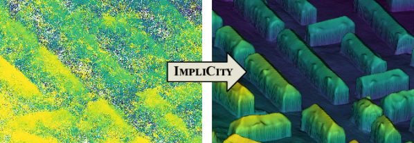
High-resolution optical satellite sensors, combined with dense stereo algorithms, have made it possible to reconstruct 3D city models from space. However, these models are, in practice, rather noisy and tend to miss small geometric features that are clearly visible in the images. We argue that one reason for the limited quality may be a too early, heuristic reduction of the triangulated 3D point cloud to an explicit height field or surface mesh. To make full use of the point cloud and the underlying images, we introduce ImpliCity, a neural representation of the 3D scene as an implicit, continuous occupancy field, driven by learned embeddings of the point cloud and a stereo pair of ortho-photos. We show that this representation enables the extraction of high-quality DSMs: with image resolution 0.5 m, ImpliCity reaches a median height error of $\approx\,$ 0.7 m and outperforms competing methods, especially w.r.t. building reconstruction, featuring intricate roof details, smooth surfaces, and straight, regular outlines.

keywords:

3D Reconstruction, Digital Surface Model (DSM), Deep Implicit Fields, Scene Representation, Satellite Imagery.

1 Introduction

Modern very high-resolution (VHR) satellite sensors have made it possible to reconstruct sub-meter resolution 3D surface models from space. They are able to collect optical images with ground sampling distances $\leq$ 0.5 m from multiple viewpoints almost anywhere on Earth. Several software packages have been developed to derive 3D models from such satellite images [krauss2013fully, de2014automatic, qin2016rpc, rupnik2017micmac, beyer2018ames, cournet2020ground, youssefi2020cars]. Typically, they adopt stereo matching algorithms originally developed for terrestrial or airborne photogrammetry. The principle of such algorithms is to find a dense set of image correspondences that have high photo-consistency and at the same time form a (piece-wise) smooth surface. After matching all suitable image pairs, the correspondences are triangulated to 3D points and fused into a single point cloud, which is commonly rasterized into a 2.5-dimensional height field (a.k.a. digital surface model, DSM) for further use.

Due to limited image resolution, sub-optimal stereo geometry, and radiometric differences caused by variable lighting and atmospheric effects, DSMs derived from satellite observations tend to be noisy (see Figure 1). Moreover, high-frequency details that would, in principle, be visible in the images are barely reconstructed. Those DSMs are thus often regarded as intermediate products and processed further, with a refinement step that aims to suppress noise and to impose a-priori assumptions about the surface, like straight building edges and vertical walls. Early attempts used low-level filtering and hand-coded rules. More recent works rely on neural networks to learn the mapping from a coarse DSM to a refined one from data [bittner2019dsm, bittner2019multi, bittner2020long, wang2021machine, stucker2022resdepth].

A fundamental property shared by different DSM reconstruction and refinement methods is an explicit representation of the surface, either as a mesh with a given number of vertices (respectively, faces) or as a regular 2D grid of height values. Such explicit parametrizations are convenient, but they do not preserve all information contained in the original point cloud and restrict the ability to resolve small structures. Recently, implicit neural functions have emerged as a powerful and effective representation of 3D geometry [park2019deepsdf, chen2019learning, mescheder2019occupancy, peng2020convolutional]. Instead of discretizing the 3D scene into a set of explicit surface elements, they implicitly model its geometry as a continuous field of occupancies or signed distance values, encoded in the weights of a neural network. The network can be evaluated at any 3D coordinate and, therefore, conceptually, allows for infinite resolution—in practice, its effective resolution is bounded by the representation power of the finite number of neurons, as well as by the resolution of the training data.

Refer to caption — Figure 1: ImpliCity is a deep, implicit representation of surface geometry. It is derived from a photogrammetric 3D point cloud and associated images. Note the geometric details on the roofs despite the substantial noise level of the input point cloud.

So far, implicit representations have been explored to model the 3D geometry of local shapes [genova2019learning, genova2020local], single objects [park2019deepsdf, atzmon2020sal], indoor scenes [jiang2020local, peng2020convolutional, sitzmann2020siren, chabra2020deep], and single buildings [chen2021reconstructing]. In this work, we go one step further and investigate their potential to accurately reconstruct 3D urban scenes, on the order of several km², from satellite data. To that end, we introduce ImpliCity, a coordinate-based, implicit neural 3D scene representation based on a point cloud derived from satellite photogrammetry. Since such point clouds are comparatively sparse and lack high-frequency detail, we additionally use an image stereo pair to guide the occupancy prediction. ImpliCity reconstructs city models with fine-grained shape details, smooth and well-aligned surfaces, and crisp edges. It thereby reduces the mean absolute error by >60% compared to a conventional stereo DSM.

2 Related Work

Deep Implicit Functions. Deep implicit functions for surface reconstruction have been proposed concurrently by [mescheder2019occupancy, park2019deepsdf, chen2019learning]. These seminal works represent a 3D shape as an implicit, continuous field $f$ , which is parametrized as a neural decoder network, and constrained by a global latent code (a \sayfeature vector of the scene) extracted with neural encoder network. The field $f$ can be queried with a 3D location $\mathbf{x}\in\mathbb{R}^{3}$ and returns either the occupancy of $\mathbf{x}$ (i.e., its probability of lying below the surface) or its signed distance to the surface. To extract an explicit surface model, one reconstructs the iso-surface $f\!=\!0.5$ of the occupancy, respectively $f\!=\!0$ for the signed distance, for instance with marching cubes [lorensen1987marching].

As the scene information is stored as a global latent code, the method described so far does not generalize to unseen objects, fails to capture local surface details, and scales poorly with scene size. Therefore, more recent works [chabra2020deep, jiang2020local, genova2020local, peng2020convolutional] decompose the scene into parts that are constrained by local codes. Moreover, [peng2020convolutional] introduce a fully convolutional encoder. In this way, the implicit representation inherits the translation equivariance of convolutions; which, in turn, enables large-scale reconstructions. [saito2019pifu] introduce local latent codes that are pixel-wise aligned with the image used for supervision, so as to obtain crisp surface edges aligned with the image gradients. The work perhaps most similar in spirit to ours is [yang2021s3], where an implicit neural model is used to reconstruct humans from LiDAR scans, guided by a (single) image to retrieve details such as the wrinkles of clothes.

Deep Implicit Functions for Satellite Images. To the best of our knowledge, [derksen2021shadow, xiangli2021citynerf] are so far the only works that have explored deep implicit representations in the context of satellite data. Both are based on the Neural Radiance Field (NeRF) method of [mildenhall2020nerf] that models an observed 3D scene as a continuous, volumetric field of viewpoint-dependent radiance values. The NeRF approach is designed primarily for novel-view synthesis, not geometrically detailed reconstruction. It does, of course, implicitly capture 3D geometry, but with an accuracy just enough to render it from new viewpoints and obtain radiometrically convincing images. E.g., the average reconstruction errors reported in [derksen2021shadow] are similar to those of conventional satellite photogrammetry. Also, the NeRF encoder must capture viewpoint-dependent appearance changes, and therefore extract implicit lighting and material information. As a consequence, it cannot generalize beyond the training region.

3 Method

Our approach starts from a set of satellite images $\mathcal{I}$ with overlapping fields of view and known camera poses. We follow best practices for satellite photogrammetry and first perform conventional, dense image matching for all suitable image pairs, followed by triangulation. See Section 4.1.

Problem Formulation. Given a set of triangulated 3D points $\mathcal{P}=\left\{\mathbf{p}_{i}\in\mathbb{R}^{3}\right\}_{i=1}^{N}$ , collected from all stereo pairs, our goal is to build a detailed and geometrically accurate 3D reconstruction of the observed scene. This is where our approach deviates from standard practice: we do not convert the raw point cloud $\mathcal{P}$ into a raster DSM for subsequent 2.5D processing. Instead, we reason in 3D space and represent the scene geometry as a continuous occupancy field. The field is represented by a function $f_{\theta}$ that, for a given 3D coordinate $\mathbf{x}\in\mathbb{R}^{3}$ , returns the probability $\hat{o}$ that the location is occupied. I.e., $f_{\theta}$ should be 0 wherever there is free space, and 1 on and underneath the surface:

f_{\theta}\big{(}\mathbf{x},\psi(\mathcal{P},\mathbf{x}),\xi(\mathcal{I},\mathbf{x})\big{)}\rightarrow\hat{o}\in[0,1]\;,

(1)

where $\psi(\mathcal{P},\mathbf{x})\in\mathbb{R}^{d}$ and $\xi(\mathcal{I},\mathbf{x})\in\mathbb{R}^{d}$ are location-dependent latent codes that modulate the occupancy probability. In our case, $\psi(\mathcal{P},\mathbf{x})$ describes the local structure of the point cloud $\mathcal{P}$ , whereas $\xi(\mathcal{I},\mathbf{x})$ encodes the local image texture at the 2D projections of $\mathbf{x}$ in two input views. Inspired by recent trends in 3D surface reconstruction, we parametrize $f_{\theta}$ as well as the feature extractors $\psi(\mathcal{P},\mathbf{x})$ and $\xi(\mathcal{I},\mathbf{x})$ as neural networks. To extract an explicit surface from this implicit representation, one must sample a sufficiently dense set of 3D locations $\mathbf{x}$ , evaluate the function $f_{\theta}$ at all of them, and extract the iso-surface $f_{\theta}=0.5$ .

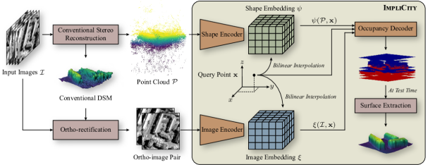
Overview. Figure 2 depicts an overview of our approach. At its core is ImpliCity, a coordinate-based neural representation of 3D scene geometry, guided by satellite images. The inputs to ImpliCity are a raw, irregular, and unoriented point cloud $\mathcal{P}$ , as obtained from satellite-based stereo reconstruction, and two ortho-rectified (panchromatic) satellite images. We first map every point in $\mathcal{P}$ to a feature vector that encodes its geometric context, then aggregate those feature vectors into a shape embedding $\psi$ . The embedding $\psi$ is aligned with the geographic coordinates, i.e., its $z$ -axis is the vertical and its $(x,y)$ -axes are the East and North directions in the local UTM zone. Similarly, we map the ortho-images to an image embedding $\xi$ with a fully convolutional 2D encoder, so as to encourage consistency between the reprojected 3D scene geometry and the image content. Note that, since the ortho-images are rectified to UTM coordinates, the shape embedding $\psi$ and the image embedding $\xi$ are, by construction, aligned and share the same $(x,y)$ -axes. With these embeddings, we can, at any location $\mathbf{x}$ , read out the two $d$ -dimensional codes $\psi(\mathcal{P},\mathbf{x}),\xi(\mathcal{I},\mathbf{x})$ and pass them, together with the coordinates, to a decoder function $f_{\theta}:\mathbb{R}^{3}\times\mathbb{R}^{d}\times\mathbb{R}^{d}\rightarrow[0,1]$ that infers the occupancy state at $\mathbf{x}$ . In our case, the decoder is a multi-layer perceptron with internal skip connections.

In the following, we introduce our network architecture (Section 3.1) and its variants (Section 3.2) in more detail before proceeding to the training procedure (Section 3.3) and the sampling strategy employed to define the training signal (Section 3.4). Finally, we describe how we convert the implicit occupancy volume into an explicit raster DSM (Section 3.5).

3.1 Network Architecture

The architecture of ImpliCity builds upon recent advances in learned, implicit 3D modeling. We adopt the convolutional single-plane encoder proposed by [peng2020convolutional] to process the input point cloud and the pixel-aligned encoder of [saito2019pifu] to process the ortho-images. As a decoder, we apply the same fully-connected network as in [peng2020convolutional].

Shape Embedding. To represent the local 3D point distribution that forms the basis for surface reconstruction, we compute a feature encoding from the point cloud $\mathcal{P}$ . We follow [peng2020convolutional] and first apply a point-wise encoder based on PointNet [qi2017pointnet], with one fully connected layer followed by five fully-connected ResNet blocks [he2016deep]. Each ResNet block includes a local pooling operation to locally aggregate 3D context information. The extracted $d$ -dimensional per-point features are then orthographically projected onto a horizontal plane and discretized into a regular 2D grid of $H\times W$ grid cells, where features that project into the same cell are averaged. In our implementation, we use a grid spacing of 0.5 m in world coordinates. Following [peng2020convolutional], the resulting feature \sayimage, with size $H\times W\times d$ , is processed further with a 2D U-Net [ronneberger2015u], equipped with symmetric skip connections to preserve high-frequency information. To capture long-range context, the depth of the U-Net is set such that its receptive field spans the entire feature image.

Satellite Image Embedding. Point clouds derived from satellite images are comparatively sparse and fairly noisy (cf. Figure 1). As a consequence, they do not preserve high-frequency details (like sharp roof edges or small dormers) that are, in principle, visible in the images. To recover fine-grained geometric details, we thus build a second latent embedding $\xi$ from a panchromatic stereo pair. That image embedding is then used as additional input to the decoder to guide the occupancy prediction. The two images of the stereo pair are aligned by ortho-rectifying both of them with the same, preliminary surface model (cf. Section 4.1) and stacked into a two-channel image. To generate $\xi$ , we process that image with an encoder similar to the stacked hourglass architecture [newell2016stacked] used in PIFu [saito2019pifu]. To adapt it for our purposes, we modify the first layer to accept our two-channel input and change the hidden feature dimension $d$ to match that of the shape embedding $\psi$ . Note that ortho-rectifying the images (i) makes it possible to work with a single image embedding despite the two different viewpoints, and (ii) ensures that the embeddings $\psi$ and $\xi$ are correctly aligned.

Occupancy Decoder. The task of the decoder is to estimate the occupancy probability at any location in scene space. Given a point $\mathbf{x}\in\mathbb{R}^{3}$ , we project it onto the horizontal $(x,y)$ coordinate plane and retrieve its shape code $\psi(\mathcal{P},\mathbf{x})$ and image code $\xi(\mathcal{I},\mathbf{x})$ from the two embeddings with bilinear interpolation. The occupancy at $\mathbf{x}$ , as a function of its coordinates $\mathbf{x}$ , shape code $\psi(\mathcal{P},\mathbf{x})$ , and image code $\xi(\mathcal{I},\mathbf{x})$ , is then predicted with a network consisting of five consecutive, fully-connected ResNet blocks. In our implementation, each ResNet block has $d$ neurons, and the sum $\psi(\mathcal{P},\mathbf{x})+\xi(\mathcal{I},\mathbf{x})$ of the two codes is added as side input to every block, as in [peng2020convolutional].

3.2 Network Variants

In our method, the stereo images are simply stacked and encoded independently of the point cloud. This raises the question whether a single image might be enough, and whether the use of images improves the reconstruction at all. To investigate these questions, we construct two network variants that differ w.r.t. the number and combination of input modalities but are otherwise identical. In particular, we keep the network architecture fixed and train each variant using the same training settings and data samples. The network configuration based on stereo guidance is our default setting, referred to as ImpliCity-stereo (or simply ImpliCity if not stated otherwise). The first variant, ImpliCity-mono, uses only a single ortho-image to generate the latent embedding $\xi$ . Therefore, it cannot exploit stereo information (in the form of misalignment between ortho-photos) and has to make do with image patterns and textures from a single image, with no redundancy. The second variant, ImpliCity-0, has no access to image information. It learns the mapping from 3D points to occupancies constrained only by the shape embedding $\psi$ , i.e., the local point distribution. Note that this configuration corresponds to the original Convolutional Occupancy Networks proposed in [peng2020convolutional].

3.3 Training and Inference

At training time, we randomly sample query points $\left\{\mathbf{x}_{i}\in\mathbb{R}^{3}\right\}$ within the volume of interest and in the vicinity of the true surface (see Section 3.4). The training is supervised by the binary cross-entropy loss $\mathcal{L}$ between the predicted occupancies $\hat{o}$ and the true occupancies $o$ at these points:

\mathcal{L}(\hat{o},o)=\sum_{i}\big{(}o_{i}\cdot\log(\hat{o}_{i})+(1-o_{i})\cdot\log(1-\hat{o}_{i})\big{)}\;.

(2)

True occupancies $o_{i}$ are derived from an existing city model of the training region. At inference time, we sample a regular 3D grid of query points in a hierarchical fashion, see Section 3.5.

3.4 Spatial Sampling

One challenge when training implicit neural shape models is to reach the right balance between expressiveness and generality, which boils down to sampling adequate 3D points $\mathbf{x}_{i}$ during training. If points were uniformly sampled in 3D space, most points would be far away from all surfaces. Consequently, the learned model would be biased towards predicting free space, as the dominant class in the absence of strong surface cues; and towards overly smooth reconstructions, since it has rarely seen surface details during training. On the other hand, if the points were exclusively sampled in the vicinity of the surface, the model would be prone to overfitting the training set, since the learning would narrowly focus on specific properties of the training area that may not generalize to other parts of the space.

In our approach, we combine uniform sampling and surface sampling, a strategy that has proven efficient for implicit neural models [saito2019pifu]. To begin with, we uniformly sample a first set of points arbitrarily within the volume of interest. Second, we densely sample a second set of points on the true surface and perturb them with zero-mean Gaussian random noise, for our data with standard deviation $\sigma\!=\!0.4\,$ m. See Section 4.1 for details. The two sets are then merged and together form the training set. In our experiments, the ratio between arbitrary points and surface points is 1:4.

3.5 Surface Extraction

To turn the implicit function $f_{\theta}$ into an explicit surface representation, we use a conventional raster DSM with a grid spacing of 0.25 m. Inspired by the Multi-resolution Iso-Surface Extraction algorithm of [mescheder2019occupancy], we employ a hierarchical refinement scheme to extract the iso-surface $\hat{o}\!=\!0.5$ from the occupancy volume. This approach makes it possible to recover a high-resolution DSM without having to densely sample the entire height range.

We start by discretizing the volume of interest into a regular grid of 3D points with a horizontal resolution equal to the grid spacing of the DSM and an initial vertical resolution of 16 m. Next, the occupancy of every grid point is predicted with the trained ImpliCity model. Using the fact that in a 2.5D DSM there is exactly one transition per pixel from free to occupied space, we mark the highest occupied 3D point per $(x,y)$ -column and the one immediately above it as active, increase the vertical resolution between the two active points by a factor 4, and predict the occupancy of the three newly generated points. Then, we again zoom in on the highest occupied point and the one immediately above it and repeat the refinement. Four iterations of this refinement lead to a final nominal resolution of 6.25 cm in the vertical direction. The highest occupied point after the last iteration is declared the DSM height $z(x,y)$ . Going down to such a low nominal resolution helps to avoid aliasing artefacts on the reconstructed surface, even though it is, of course, far below the effective vertical resolution achievable with satellite images of $\approx\,$ 0.5 m GSD at nadir.

4 Experiments

4.1 Dataset and Preprocessing

Imagery and Study Area. We evaluate our method on panchromatic satellite images acquired over Zurich, Switzerland. We have one WorldView-3 and 14 WorldView-2 images at our disposal. They were captured between 2014 and 2018, with 22 days the shortest time interval between two acquisitions. The average GSD is $\approx\,$ 0.5 m at nadir. The study area¹¹1The area corresponds to ZUR1 of [stucker2022resdepth]. covers 4 km² and includes widely spaced, detached residential buildings, allotments, and high commercial buildings. Moreover, it contains a stretch of the river Limmat and a forested hill. In analogy to [stucker2022resdepth], we split the area into five equally large, mutually exclusive stripes and allocate three stripes for training, one for validation, and one for testing.

Point Cloud Generation. We use a re-implementation of state-of-the-art hierarchical semi-global matching [rothermel2012sure], tailored to satellite images, to generate the input point cloud $\mathcal{P}$ . First, we employ the method of [patil2019new] to perform bias correction of the supplied rational polynomial coefficient (RPC) projection models. Next, we determine suitable image pairs for dense matching based on heuristics inspired by [facciolo2017automatic, qin2019critical]. Starting from all possible image pairs, we eliminate those whose intersection angles in object space are <5^∘ or >30^∘ (measured at the center of the region of interest), or whose incidence angles are >40^∘ (mean of the two images). We further discard image pairs whose difference in sun angle is >35^∘. To leverage the redundancy in the image set as much as possible, we use all remaining image pairs for pairwise rectification and pairwise dense matching, irrespective of differences in acquisition time, as suggested by [krauss2019cross]. After matching, we use the inverse RPC projection function to triangulate corresponding points per image pair, resulting in 26 stereo clouds in the same scene coordinate system, which we simply merge into a single point cloud $\mathcal{P}$ .

Initial DSM Reconstruction. Besides the point cloud $\mathcal{P}$ , ImpliCity receives two ortho-rectified panchromatic satellite images as input. For the ortho-rectification, we require an initial surface estimate of the observed scene. To generate it, we fuse the point cloud $\mathcal{P}$ into a coherent multi-view raster DSM with a grid spacing of 0.25 m, by computing the cell-wise median of the $n$ highest 3D points, where $n$ is defined as the average number of 3D points per grid cell [rothermel2016]. Further, we adopt standard post-processing operations from aerial and satellite-based photogrammetry to denoise the DSM, remove spikes, and fill cells without a valid height with inverse distance weighted (IDW) interpolation.

Stereo Pair Selection and Rectification. Among all available image pairs with adequate stereo geometry (see above), we determine a single best pair that serves as the second input to ImpliCity. The selection is based on three criteria, namely low intersection angle, small time difference between acquisitions (similar season), and low cloud coverage. Like [stucker2022resdepth], we ortho-rectify the two selected images with the help of the initial DSM, without ray-casting to detect occlusions. Instead, duplicate gray-values are rendered for rays that intersect the surface twice, leading to systematic patterns of repeated, photometrically inconsistent textures. Due to the small baseline between the two views, discrepancies between the ortho-images (except for illumination and atmospheric effects) primarily stem from height errors in the initial DSM rather than from viewpoint differences.

Ground Truth Occupancy. To train our method, we need to know the true occupancy of any 3D spatial location sampled within the volume of interest. Fortunately, such full 3D supervision can be readily derived from the publicly available city model of Zurich [zurich-model]. The model has been created by the municipal surveying department in a semi-automatic manner, by fusing airborne laser scans, building and road boundaries (including bridges) from national mapping data, and roof models derived by manual stereo digitization. The height accuracy is specified as $\pm$ 0.2 m for buildings and $\pm$ 0.4 m for terrain.

We densely sample points on roofs, facades, and terrain of the city model. The average distance between nearest points amounts to 0.2 m for points sampled on facades and terrain. For points sampled on roofs, we increase the sampling resolution to 0.1 m to capture geometric details such as dormers with higher fidelity. Furthermore, we uniformly sample points within the volume of interest with a mean distance of $\approx\,$ 1.0 m between points. Points sampled on the surface are assigned true occupancy values of 1; points sampled in free space are assigned 0 or 1, depending on whether they lie above or below the surface.

4.2 Implementation Details

We randomly sample training patches with a spatial dimension of 64 $\times$ 64 m in world coordinates from the training region. To avoid biases due to the specific topography and urban layout, we augment the data by randomly rotating the training patches by $\alpha\in\{0^{\circ},90^{\circ},180^{\circ},270^{\circ}\}$ and random flipping along the $x$ and $y$ axes. At inference time, we reconstruct large-scale scenes by applying the learned model in a sliding window.

We follow best practice and normalize the data (point cloud, ortho-images, query points) for neural network training. Every 64 $\times$ 64 m patch, originally given in UTM coordinates (zone 32T), is first horizontally shifted and scaled such that all point coordinates lie in $[0,1]$ . Then, all points are vertically centered to the median height and rescaled with a fixed factor. That factor is found by computing standard deviations of the heights for 20’000 random patches from the training set and averaging them (cropped to the \nth5 and \nth95 percentile for robustness). Ortho-images are normalized with the mean and standard deviation over the intensity values of all training pixels.

We have implemented ImpliCity in PyTorch and run it on a NVIDIA GeForce GTX 2080 Ti GPU. Source code and pretrained models are available at https://github.com/prs-eth/ImpliCity. In all experiments, we use a hidden feature dimension $d$ of 32 for both encoders and the joint decoder, and feature plane dimensions 128 $\times$ 128 for the shape embedding $\psi$ and 64 $\times$ 64 for the image embedding $\xi$ . For training, we employ the ADAM optimizer with a base learning rate of $5\cdot 10^{-5}$ ( $\beta_{1}$ =0.9, $\beta_{2}$ =0.999), no weight decay, and a cyclical learning rate scheduler [smith2017cyclical] with cycle amplitude $5\cdot 10^{-4}$ . We set the batch size to 1 but accumulate gradients for 64 training iterations before performing back-propagation. Errors at water and forest pixels are down-weighted by a factor of 0.5 when computing the loss (Eq. 2). We stop training once the DSM metrics (cf. Section 4.4) on the validation set have converged. We experimentally found that reconstruction quality improves when areas with evident temporal differences between the satellite imagery and the city model are masked out during training.

4.3 Baselines

We compare ImpliCity against the following baselines:

Initial DSM: The raster DSM generated from the input point cloud $\mathcal{P}$ , representative of conventional satellite-based reconstruction (see Section 4.1 for details).

ResDepth: A learned DSM refinement approach by [stucker2022resdepth] that directly refines the initial raster DSM with a U-Net [ronneberger2015u]. ResDepth-0 is trained to regress an additive height correction at every pixel. The image-guided variants ResDepth-mono and ResDepth-stereo exploit one and two ortho-images as additional input to guide the refinement.

PIFu: The Pixel-aligned Implicit Function (PIFu) method of [saito2019pifu], representative for deep, implicit surface reconstruction from images. We feed the initial DSM as input to the network. This baseline, denoted PIFu-0, corresponds to learned DSM filtering with the help of an implicit neural scene representation. Moreover, we train PIFu-mono and PIFu-stereo variants with one, respectively two ortho-images as additional input channels. To remain consistent with the other methods, we use a patch size of 256 $\times$ 256 pixels (64 $\times$ 64 m in scene space) rather than 512 $\times$ 512 as in the original PIFu.

4.4 Quality Metrics

We use the publicly available city model of Zurich [zurich-model] to evaluate the performance of ImpliCity. That city model is delivered in the form of 2.5D building models and a terrain surface. Therefore, we resort to 2.5D metrics commonly used for DSM evaluation. Regions where the city model differs from the images due to recent construction activities have been masked out. We render a reference DSM from the city model to measure the mean absolute error (MAE), the root mean square error (RMSE), and the median absolute error (MedAE), computed over per-pixel deviations between predicted and reference heights.²²2These widely used pixel-wise metrics do not fully characterize DSM quality: improved reconstruction of intricate geometric details may not be reflected in lower errors, see Sec. 4.5. For a more in-depth analysis, we calculate the metrics separately for building and terrain pixels (according to the ground truth), where the building mask has been dilated by two pixels (0.5 m) to ensure that distortions along its contours are reflected in the building error. Moreover, we differentiate between general terrain and forested areas with the help of a manually created forest mask.

ImpliCity: City Modeling from Satellite Images with Deep Implicit Occupancy Fields