Abstract

Expectation Maximization (EM) is the standard method to learn Gaussian mixtures. Yet its classic, centralized form is often infeasible, due to privacy concerns and computational and communication bottlenecks. Prior work dealt with data distributed by examples, horizontal partitioning, but we lack a counterpart for data scattered by features, an increasingly common scheme (e.g. user profiling with data from multiple entities). To fill this gap, we provide an EM-based algorithm to fit Gaussian mixtures to Vertically Partitioned data (VP-EM). In federated learning setups, our algorithm matches the centralized EM fitting of Gaussian mixtures constrained to a subspace. In arbitrary communication graphs, consensus averaging allows VP-EM to run on large peer-to-peer networks as an EM approximation. This mismatch comes from consensus error only, which vanishes exponentially fast with the number of consensus rounds. We demonstrate VP-EM on various topologies for both synthetic and real data, evaluating its approximation of centralized EM and seeing that it outperforms the available benchmark.

1 INTRODUCTION

Expectation Maximization (EM) is both the standard method for density estimation of Gaussian Mixture Models (GMMs) and a popular clustering technique. Yet these two key tasks do not constitute an exhaustive list of EM applications. From its formalization (Dempster et al., 1977) up to today, EM has been widely employed, with applications ranging from semi-supervised learning (Ghahramani and Jordan, 1993) to topic modeling (Blei et al., 2003). EM remains an active research subject, as seen in the prolonged effort to study its convergence, from Wu (1983) until today (Balakrishnan et al., 2014; Daskalakis et al., 2017; Kunstner et al., 2021).

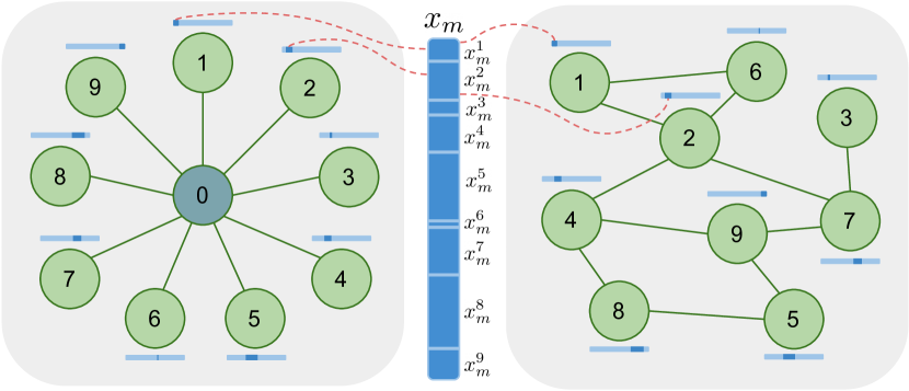
Figure 1: Each example $x_{m}$ is partitioned by features, either in federated learning (left) or fully decentralized (right) networks of agents. We want an unsupervised learning algorithm that allows the agents to perform density estimation and clustering in collaboration without requiring their data to be centralized.

Employing EM to fit GMMs, a textbook application, is a particularly popular unsupervised learning tool. This density estimation is used to model subpopulations and approximate densities—even mixtures of diagonal Gaussians, given enough components, can approximate generic densities to an arbitrary error (Sorenson and Alspach, 1971)—making Gaussian mixtures exceptionally expressive models. Further, GMMs allow for ellipsoidal clustering, making them more flexible than the spherical clusters of the popular $k$-means algorithm. Moreover, while $k$-means performs hard clustering, GMMs allows for soft clustering, expressing uncertainty associated with the clustering and handling clusters that are not mutually exclusive.

However, data is often too large, privacy sensitive, or both, preventing the use of a data center where conventional, centralized methods can be employed. Such setups call for distributed approaches where data is treated while partitioned. The partitioning may come from a pre-processing step to cope with the scale of data (Mann et al., 2009), but it may also be the original layout of data collected by multiple entities (Nedić and Ozdaglar, 2010). In either case, distributed learning allows us to spread computational costs which are too high for a single agent. Further, without privacy guarantees, it is often impossible for different entities to collaborate and learn from joint data. Yet, even when their data cannot be routed to a single agent (regardless of its size), exchanging a summarized, non-invertible function of the data may be acceptable. Thus, avoiding centralization circumvents privacy concerns. Distributed learning is also key in systems where high speed is paramount (Li et al., 2012) and communication delays prevent centralized approaches.

Scenarios requiring distributed approaches include large networks, like edge computing applications and personalized models (Wang et al., 2019), and networks with fewer agents, such as organizations (e.g. healthcare systems (Rieke et al., 2020)) with siloed data.

One distributed learning scheme that has been drawing a remarkable amount of attention, both in academia and in industry, is Federated Learning (FL) (McMahan et al., 2017), where multiple agents (clients) collaborate to learn a shared model under the coordination of a central server without sharing their local data. This scheme is characterized by a star communication graph and a server-client architecture (see Figure 1). Nevertheless, FL has some limitations, such as having a single point of machine failure and being prone to communication bottlenecks (Lian et al., 2017) as pointed out in Kairouz et al. (2021).

The more general fully decentralized learning circumvents these issues by having no central parameter server (agents form a peer-to-peer network, see Figure 1). Fields like multi-agent control and wireless sensor networks employ extensive work on optimization under fully decentralized schemes, such as Olshevsky and Tsitsiklis (2009); Nedic and Ozdaglar (2009); Duchi et al. (2012); Qu and Li (2018), and references therein. While these works are often formulated as generic optimization problems, rather than designed for a specific learning task, they tend to be motivated by applications where data is distributed by examples (horizontally partitioned), as is made clear, for example, in Forero et al. (2010). Closer to our work, multiple fully decentralized algorithms use EM to fit GMMs in horizontally partitioned setups, such as Nowak (2003); Kowalczyk and Vlassis (2005); Gu (2008); Forero et al. (2008); Bhaduri and Srivastava (2009); Safarinejadian et al. (2010); Weng et al. (2011); Altilio et al. (2019). Related density estimation tasks have also been considered (Hu et al., 2007; Hua and Li, 2015; Dedecius and Djurić, 2017).

In these horizontally partitioned settings, loss functions tend to naturally decouple across agents. Yet in many applications, such as online shopping records data and social network interactions, the features are collected across different providers. In these setting, or when the number of examples, $M$, and their dimension, $d$, verify $d\gg M$, as in the natural language processing and bioinformatics applications in Boyd et al. (2011), the data benefits from Vertical Partitioning (VP) (Yang et al., 2019).

The flexible fully decentralized VP learning, in specific, allows us to cope with the arbitrary communication graphs observed in IoT, teams of robots, and wireless sensor networks applications too. (E.g., agents deployed to learn the behavior of a random field across a region, such as the concentration of a pollutant.) The literature for the VP setting is not as abundant as its horizontal counterpart. Vaidya and Clifton (2003) tackle VP $k$-means clustering, focusing on privacy, rather than aiming for full decentralization; Grozavu and Bennani (2010) perform VP clustering resorting to self-organizing maps; Ding et al. (2016) addresses $k$-means clustering for FL; and Fagnani et al. (2013) deals with density estimation, assuming a restricted GMM where each agent is associated with a component of the mixture. Note that these and our work consider unsupervised learning, yet VP supervised learning has also been studied (e.g. Ying et al., 2018). For more VP learning algorithms, see Yang et al. (2019).

We present an EM-based method for fitting Gaussian mixtures to VP data both in federated learning and fully decentralized setups (VP-EM), allowing for the scalability and privacy we set out to achieve. These setups are illustrated in Figure 1, where the agents may represent anything from companies to sensors.

Our main contributions are as follows:

• Formulating the task of fitting GMMs in vertically partitioned schemes and identifying its challenges;

• Proposing a solution to these challenges by partitioning parameters and constraining their space;

• Framing the VP-EM algorithm for FL setups, with the same monotonicity guarantee as the classic EM;

• Extending VP-EM to peer-to-peer setups, coping with additional challenges and exploring the topology to offer a range of data sharing options;

• Equipping VP-EM with stopping criteria.

2 EM AND GAUSSIAN MIXTURES

EM performs (local) maximum likelihood estimation in models where the likelihood function for parameter $\theta$ depends on observed data $X$, but also on latent variables $Z$,

$$\mathcal{L}(\theta)=\log p\left(X\,|\,\theta\right)=\log\sum_{Z}p\left(X,Z\,|\,\theta\right).$$ (1)

For mixture models, $Z$ often indicates the mixture component which, if known, would make the likelihood function concave, with a closed-form solution. (For missing data, $Z$ corresponds to missing portions of the examples.) Yet, in reality, $Z$ is a random variable, thus maximizing the complete-data likelihood $p\left(X,Z\,|\,\theta\right)$ is not a well-posed problem. However, if we fix $\theta$ to some $\theta^{t}$, we can infer $Z$ using its posterior $p\left(Z\,|\,X,\theta^{t}\right)$ and computing the expected complete-data likelihood (E-step), thus defining a surrogate objective,

$$\mathcal{Q}\left(\theta\,|\,\theta^{t}\right)=\mathbf{E}_{Z|X,\theta^{t}}\left[\log p(X,Z\mid\theta)\right].$$

With a well-defined objective, we update $\theta$ using standard optimization tools (M-step), solving

$$\theta^{t+1}=\text{argmax}_{\theta}\,\mathcal{Q}\left(\theta\,|\,\theta^{t}\right).$$

After initializing $\theta$, the EM iterates between E- and M-steps until some stopping criterion is met.

Theorem 1.

The EM is monotonically non-decreasing on its objective,

$$\mathcal{L}\left(\theta^{t+1}\right)\geq\mathcal{L}\left(\theta^{t}\right).$$

This property, shown in Dempster et al. (1977), often results in convergence of (1) to a (local) maximizer.

A GMM with $K$ components, combined with weights $\left\{\pi_{k}\right\}_{k=1}^{K}$ on the probability simplex, has the density

$$p_{\theta}(x)={\textstyle\sum\nolimits_{k=1}^{K}}\pi_{k}\,{\mathcal{N}}\left(x;\mu_{k},\Sigma_{k}\right),$$ (2)

where $x,\mu_{k}\in{\mathbf{R}}^{d}$, $\Sigma_{k}\in{\mathbf{R}}^{d\times d}$, $\theta=\left\{\pi_{k},\mu_{k},\Sigma_{k}\right\}_{k=1}^{K}=\left\{\pi,\mu,\Sigma\right\}$, and the Gaussian distribution is given by

$${\mathcal{N}}\left(x;\mu,\Sigma\right)=\lvert 2\pi\Sigma\rvert^{-\frac{1}{2}}\exp\left(-(x-\mu)^{T}\Sigma^{-1}(x-\mu)/2\right).$$ (3)

When using EM to fit a GMM to $\mathcal{X}=\{x_{m}\}_{m=1}^{M}\subseteq\mathbf{R}^{d}$, we have $\mathcal{Z}=\{z_{m}\}_{m=1}^{M}$, where $z_{m}\in\mathbf{R}^{K}$ indicates the component from which $x_{m}$ is sampled. The E-step boils down to updating the parameters of the posterior

$${\gamma}_{mk}^{t+1}=\mathbf{E}_{Z|X,\theta^{t}}\left[z_{mk}\right]\propto\tilde{\gamma}_{mk}^{t+1}=\pi_{k}^{t}{\mathcal{N}}\left(x_{m};\mu_{k}^{t},\Sigma_{k}^{t}\right),$$ (4)

where ${\gamma}_{mk}^{t}$ is obtained by normalizing $\tilde{\gamma}_{mk}^{t}$ over $k$. This step performs a soft assignment of each example $m$ to each cluster $k$ (notice ${\gamma}_{mk}^{t+1}\geq 0$ and $\mathbf{1}^{T}{\gamma}_{m}^{t+1}=1$). ${\gamma}_{mk}^{t}$ is called the responsibility that component $k$ takes for $x_{m}$ at iteration $t$.

The M-step updates the GMM parameters as follows:

$${\textstyle\pi_{k}^{t+1}=} {\textstyle\frac{1}{M}\sum\nolimits_{m=1}^{M}\gamma_{mk}^{t+1}},$$ (5a)

$${\textstyle\mu_{k}^{t+1}=} {\textstyle\frac{1}{M\pi_{k}^{t+1}}\sum\nolimits_{m=1}^{M}\gamma_{mk}^{t+1}x_{m}},$$ (5b)

$${\textstyle\Sigma_{k}^{t+1}=} {\textstyle\frac{1}{M\pi_{k}^{t+1}}\sum\nolimits_{m=1}^{M}\gamma_{mk}^{t+1}\left(x_{m}-\mu_{k}^{t+1}\right)\left(x_{m}-\mu_{k}^{t+1}\right)^{T}}.$$ (5c)

A more detailed analysis of EM and its application to GMM can be found, for example, in Bishop (2006).

3 DISTRIBUTED AVERAGING CONSENSUS

Let $\psi\in{\mathbf{R}^{N}}$ be scattered across a set of $N$ agents in an undirected communication graph $\mathcal{G}=\left({\mathcal{V}},{\mathcal{E}}\right)$, where $\mathcal{V}=\{n\}_{n=1}^{N}$ is the vertex set and and $\mathcal{E}\subseteq\mathcal{V}^{2}$ is the edge set, with $\{n,n^{\prime}\}\in\mathcal{E}$ if and only if $n$ and $n^{\prime}$ are connected in the graph. Entry $\psi_{n}$ is held by agent $n$.

Distributed averaging consensus, or simply consensus (Saber and Murray, 2003; Xiao and Boyd, 2004), delivers an approximate average to all agents, $\langle\psi\rangle=\mathbf{1}^{T}\psi/N$. This is achieved by an iterative update of the state of each agent, initialized as $z_{n}^{0}=\psi_{n}$, by combining it linearly with the states of its neighbors,

$$z^{s+1}=Wz^{s},$$ (6)

where $z^{s}=(z_{1}^{s},\dots,z_{N}^{s})\in{\mathbf{R}}^{N}$ is the state of the network. The sparsity pattern of weight matrix $W$ matches the underlying communication graph, that is, $\{n,n^{\prime}\}\not\in{\mathcal{E}}\implies W_{nn^{\prime}}=0$, thus ensuring the consensus update (6) requires local communications only (i.e., between neighbors). Further, we need $W$ to be a symmetric matrix with eigenpair $(1,\mathbf{1})$ and all other eigenvectors (which are not proportional to ${\mathbf{1}}$) associated with eigenvalues whose absolute value is strictly less than 1. These properties are secured, for example, by having $W$ be the Metropolis weights matrix, or by taking $W=I-\alpha L$, where $L$ is the Laplacian of the graph and $\alpha\in\left(0,\lambda_{\max}(L)\right)$ is a constant. For more details on Metropolis weights and graph spectral theory see, e.g., Chung (1994); Xiao et al. (2005). For such $W$, repeated application of (6) brings the state of all agents to the average of the distributed data, that is, $\lim_{s\rightarrow+\infty}z^{s}=\langle\psi\rangle{\mathbf{1}}.$ Further, although exact agreement of the agents on $\langle\psi\rangle$ is only guaranteed as the number of iterations $s$ approaches infinity, consensus converges exponentially fast. Thus, in practice, we can stop consensus after a finite number of iterations, say $S$, with $z_{n}^{S}\approx\langle\psi\rangle$ at each agent $n$.

4 CHALLENGES OF LEARNING GMMS FROM DATA DISTRIBUTED BY FEATURES

As in Figure 1, let $\mathcal{X}=\{x_{m}\}_{m=1}^{M}$ be a dataset where each example $x_{m}$ is distributed across $N$ agents connected by a undirected communication graph $\mathcal{G}$,

$$x_{m}=(x_{m}^{1},\dots,x_{m}^{n},\dots,x_{m}^{N})\in\mathbf{R}^{d},$$ (7)

where agent $n$ holds partition $x_{m}^{n}\in\mathbf{R}^{d_{n}}$ for all $m$. One challenge of such partitioning is that, in contrast to the horizontal counterpart, the data is generally not iid across agents. This, in turn, is often reflected in loss functions that do not naturally decouple across agents.

If we naively run the EM on such setup, multiple problems come up, the first being the issue of storing the model parameters $\theta=\left\{\pi_{k},\mu_{k},\Sigma_{k}\right\}_{k=1}^{K}$ and the responsibilities $\gamma\in\mathbf{R}^{M\times K}$. Each entry $\gamma_{mk}$ is associated with an entire data point $m$ and mixture component $k$, having no feature-associated dimension that scatters naturally in our setting, thus each agent holds all of $\gamma$. Since we seek scalability and privacy along features, not examples (although, as mentioned later, a batch VP-EM removes dependencies on $M$), this is not a problem. In contrast, $\theta$ has feature-specific information, thus storing all of $\theta$ in each agent would lead to memory requirements proportional to $d$ on the agents, namely through $\mu_{k}\in\mathbf{R}^{d}$ and (worse) $\Sigma_{k}\in\mathbf{R}^{d\times d}$. Although memory costs are often not the main bottleneck, we want to avoid this dependency, mainly due to its implications for computational and communication costs, which we now see by examining an EM iteration.

Let us see how to partition $\theta^{t}$ across the network. From (4) and (3), we get, with a slight abuse of notation in the equality (we drop the $2\pi$ term, which cancels out when normalizing), that the E-step requires computing

$$\log\tilde{\gamma}_{mk}^{t+1}=\log\pi_{k}^{t}-\frac{1}{2}\log\lvert\Sigma_{k}^{t}\rvert-\frac{1}{2}\left\lVert x_{m}-\mu_{k}^{t}\right\rVert_{(\Sigma_{k}^{t})^{-1}}^{2},$$ (8)

where $\left\lVert v\right\rVert_{A}^{2}=v^{T}Av$. Note that $\log\pi_{k}^{t}$ is innocuous, as it does not depend on $d$. Further, $x_{m}-\mu_{k}^{t}$ does depend on $d$, but it can computed distributedly by partitioning $\mu_{k}$ such that each agent $n$ holding $x_{m}^{n}$ stores the corresponding $\mu_{k}^{n}$ for all $k$. The troublemaker is $\Sigma_{k}^{t}$. Notice how all computations involving this term (determinant, inverse, and quadratic product) hinder a distributed E-step, coupling entries that respect features observed at arbitrary nodes in the network. To deal with these challenges, on top of partitioning $\Sigma_{k}^{t}$, we see we may need to approximate it, decoupling the determinant and inverse into smaller terms of size independent from $d$ and preventing $(\Sigma_{k}^{t})^{-1}$ from coupling arbitrary entries of $x_{m}-\mu_{k}^{t}$ in the quadratic product.

In the M-step, we see from (5a) that we can locally update $\pi_{k}$ in all agents, using the local $\gamma$, thus all agents keep $\pi$, as the EM iterates. Likewise, (5b) confirms that the aforementioned partitioning of $\mu_{k}$ is viable, since $n$ holds all the terms required to update $\mu_{k}^{n}$ with

$${\textstyle\left(\sum\nolimits_{m=1}^{M}\gamma_{mk}^{t+1}(x_{m})_{n}\right)/\left(M\pi_{k}^{t+1}\right)}.$$ (9)

In (5c), $\Sigma_{k}$ raises another problem. We see its partitioning and approximation must decouple the outer product. Imposing some sparsity on $\Sigma_{k}$ emerges as an appealing approach, since entries assumed to be zero need not be estimated. We will see that an appropriate sparsity can indeed decouple the outer product.

We conclude that, to avoid communications between arbitrary agents in the network, we must allocate $\mu$ and $\Sigma$ taking into consideration where in the graph each feature is observed. For $\mu$, we saw that a simple partitioning, similar to that of the data, suffices for the EM to iterate distributedly. The following sections will detail how to partition $\Sigma$.

5 VP-EM FOR FEDERATED LEARNING

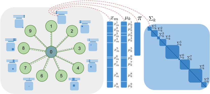
Figure 2: The VP-EM for federated learning. The E-step requires communications between clients and server (solid line), while the M-step requires local client computations only (dashed line): we alternate between a local step and a connected one. Data and model parameters are partitioned, with the darker blue representing the portions at each client. Since $\gamma$ is neither, we omit it, but it is held in its entirety at every client. All $m$ and $k$ have the same partitioning.

Let $\mathcal{X}$ be scattered over a network of data centers, as in (7). The server, node $0$, is connected to all clients, nodes $n=1,\dots,{N}$, which have no direct communication channels between them, that is, $\mathcal{E}=\left\{\left\{0,1\right\},\left\{0,2\right\},\dots,\left\{0,N\right\}\right\}$. Each client $n$ holds copies of $\gamma$ and $\pi$, as well as the partition $\mu_{k}^{n}\in\mathbf{R}^{d_{n}}$ for all $k$. (We omit the EM iteration superscript to avoid clutter.) In FL, we overcome the challenges associated with $\Sigma_{k}$ by constraining it to be a block-diagonal matrix where each block $\Sigma_{k}^{n}\in\mathbf{R}^{d_{n}\times d_{n}}$ matches the features of $x_{m}^{n}$. Entry $(i,j)$ of $\Sigma_{k}$, $[\Sigma_{k}]_{ij}$, is assumed zero when features $i$ and $j$ are observed by different clients, as seen in Figure 2.

Algorithm 1 VP-EM for Federated Learning

Input: $X$
Parameter: $K$
Output: ${\textstyle\hat{\theta}=\left\{\hat{\pi}_{k},\hat{\mu}_{k},\hat{\Sigma}_{k}\right\},\,\hat{\gamma}}$

1:Choose $\theta^{0}=\left\{\pi^{0},\mu^{0},\Sigma^{0}\right\}$ $\triangleright$ Same $\pi^{0}$ across agents

2:for $t=0,1,\dots$ do

3:     for $m\in[M]$, $k\in[K]$ do $\triangleright$ E-step (update $\gamma$)

4:         Each client $n$ locally computes its term

5:          in (10) and sends it to the server;

6:         Server adds the $N$ terms and returns (10)

7:          to the clients;

8:         Each client computes (8) locally and

9:          normalizes over $k$, arriving at (4);      

10:     Each client $n$ computes (5a), (9), and (11),

11:     updating $\theta_{n}$; $\triangleright$ M-step ($\theta^{t}\leftarrow\theta^{t+1}$)

12:     if converged then

13:         break      

14:return $\theta^{t}$, $\gamma$

Note that $[\Sigma_{k}]_{ij}=0$ does not mean features $i$ and $j$ are independent, as we are dealing with GMMs. (That would be true if $K=1$.) This structure simplifies the inversion of $\Sigma_{k}$ to a block-wise inversion and its determinant to a product of determinants of the blocks, $\lvert\Sigma_{k}\rvert=\prod_{n=1}^{N}\lvert\Sigma_{k}^{n}\rvert$, decoupling $\log\lvert\Sigma_{k}\rvert$ as a sum over agents. A similar decoupling over $n$ is obtained in the quadratic term in (8). Thus, in the E-step, the server performs a single sum,

$${\textstyle\sum_{n=1}^{N}\log\lvert\Sigma_{k}^{n}\rvert+\left\lVert x_{m}^{n}-\mu_{k}^{n}\right\rVert_{\left(\Sigma_{k}^{n}\right)^{-1}}^{2},}$$ (10)

which is then sent to the clients who, in turn, multiply it by $-{1}/{2}$, add their local copy of $\log\pi_{k}$, and normalize over $k$ locally, arriving at $\gamma_{mk}$.

From (5c), since only non-zero entries must be estimated, we see the outer product now decouples, allowing each agent $n$ to update $\Sigma_{k}^{n}$ locally with

$${\textstyle\frac{1}{M\pi_{k}}\sum\nolimits_{m=1}^{M}\gamma_{mk}\left(x_{m}^{n}-\mu_{k}^{n}\right)\left(x_{m}^{n}-\mu_{k}^{n}\right)^{T}.}$$ (11)

Algorithm 1 outlines VP-EM for federated learning, where $[a]=\{1,\dots,a\}$ and $\theta_{n}$ are the parameters stored by agent $n$, $\{\pi_{k},\mu_{k}^{n},\Sigma_{k}^{n}\}_{k=1}^{K}$. Note that, as depicted in Figure 2, only the E-step requires communications and that each data partition remains in the agent that observed it. For implementation purposes, we propose tracking the log-likelihood, $\mathcal{LL}$, using its diminishing increment as a stopping criterion , as is often done in classic EM. $\mathcal{LL}$ is obtained as a byproduct of the E-step, requiring no additional communications (see supplementary material for further details).

Corollary 1.

The VP-EM algorithm for federated learning is monotonically non-decreasing on its objective,

$$\mathcal{L}\left(\theta^{t+1}\right)\geq\mathcal{L}\left(\theta^{t}\right).$$

This follows directly from Theorem 1, given that VP-EM matches the EM when constrained to a subspace.

Importantly, we can drop the dependency on $M$ of the computational complexity of each EM iteration. We do this by updating only a subset of the entries of $\gamma$ in the E-step, which, in turn, allows for an online update of the parameters in the M-step, since only the associated subset of the terms in the sums in (5a), (5b), and (5c) changes. This batch version of VP-EM follows directly from the application of the incremental version of the EM (Neal and Hinton, 1993) and is explained in greater detail in the supplementary material.

6 VP-EM FOR FULLY DECENTRALIZED LEARNING

Let $\mathcal{X}$ be (again) scattered across a communication graph, as in (7). We now handle arbitrary graph topologies, assuming only that $\mathcal{G}$ is connected. This section can be seen as an extension of the VP-EM for FL, as it based on similar assumptions. Yet now we (1) cope with fully decentralized sums; (2) allow for less sparsity to be imposed on $\Sigma_{k}$ when privacy concerns permit. To achieve the latter point while still attaining a block-diagonal structure, we exploit the flexibility of the communication graphs describing fully decentralized setups. In particular, we explore the fact that the richer topologies allow for informative notions of locality, based on the distance (number of hops) to the agent observing each feature. This allows us to think in terms of a degree of privacy. (In FL, all clients were a hop away from the server, so moving the data even one hop away from the clients observing it leads to centralization in the server.)

But how do we choose the new block-diagonal structure of $\Sigma_{k}$? First, note we can still employ the sparsity constraint used in FL ($[\Sigma_{k}]_{ij}\neq 0$ when features $i$ and $j$ are observed by the same agent). In fact, this is our only option when privacy concerns forbid any data sharing. We call this a $0$-hop scheme, as it allows for the communication of features to agents within $0$ hops of the one observing them, $\{\}$. (See Figure 3.) Yet, when some local data sharing is allowed, we should explore this, leveraging the richer graph topologies to define a notion of distance to the node observing each feature, which can be used to estimate more entries $\Sigma_{k}$ while keeping a block-diagonal structure. Graph clustering (Schaeffer, 2007) proves useful. We propose a simple procedure to choose the blocks of $\Sigma_{k}$, which runs only once, before the EM-based iterations.

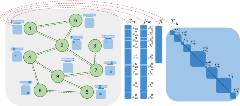
Figure 3: The VP-EM for fully decentralized learning. The E-step requires local communications (solid line), while the M-step does not (dashed line): we alternate between a local step and a connected one. Data and model parameters are partitioned, with the darker blue representing the portions at each agent. Since $\gamma$ is neither, we omit it, but it is held in its entirety at each agent. All $m$ and $k$ follow the same partitioning. We represent $\Sigma_{k}$ for the $0$-hop scheme to avoid clutter in the illustration of $\Sigma_{k}$. A diagram contrasting the sparsity of $\Sigma_{k}$ for $0$-hop and $1$-hop schemes (less sparse) can be found in the supplementary material.

Graph Clustering.

We want to choose the largest blocks possible for $\Sigma_{k}$, to constrain our search space the least possible, while respecting a degree of privacy requirement expressed by $h$ when opting for an $h$-hop communication scheme. The graph clustering algorithm takes as input the graph $\mathcal{G}$ and outputs the sparsity pattern of a (block-diagonal) matrix. For $1$-hop data sharing, the $b$th cluster (or hub), $\mathcal{H}_{b}$, corresponds to the union of some node $n$ with its neighbors $\mathcal{N}_{n}$, $\mathcal{H}_{b}=n\cup\mathcal{N}_{n}$. In general, $h$-hop hubs include all nodes up to $h$ hops away from the root node $n$. The algorithm is greedy, picking the largest $h$-hop hub in the graph and extracting it (settling ties at random). For $1$-hop hubs, this means picking the node with the highest degree (number of neighbors). We find and extract the first hub, $\mathcal{H}_{1}$, such that $\text{root}(\mathcal{H}_{1})=\operatorname*{argmax}_{n\in\mathcal{V}}\lvert\mathcal{N}_{n}\rvert$. Let $p_{1}=\lvert\mathcal{H}_{1}\rvert$, nodes in $\mathcal{H}_{1}$ are assigned numbers $1,2,\ldots,p_{1}$ in some order. We repeat the process for the residual graph, $\text{root}(\mathcal{H}_{2})=\operatorname*{argmax}_{n\in{\mathcal{V}}-{\mathcal{H}}_{1}}\lvert\mathcal{N}_{n}\rvert$, where $\mathcal{N}_{n}$ are now the neighbors in ${\mathcal{V}}-{\mathcal{H}}_{1}$, extracting ${\mathcal{H}}_{2}$. Let $p_{2}=\lvert\mathcal{H}_{2}\rvert$, nodes in ${\mathcal{H}}_{2}$ are assigned numbers $p_{1}+1,\ldots,p_{1}+p_{2}$. We repeat the process until the residual graph is void. For $1$-hop schemes, each hub is a star-shaped graph: a node stands at the root and its neighbors, the leaf nodes, surround it. We assume $[\Sigma_{k}]_{ij}=0$ when features $i$ and $j$ are observed by nodes in different hubs, obtaining a block-diagonal $\Sigma_{k}$ with blocks $\left\{\Sigma_{k}^{b}\right\}_{b=1}^{B}$ for all $k$, where $B$ is the number of hubs (and thus blocks) obtained. This procedure can be run in a distributed manner, by finding the maximum degree of the network via flooding.

Algorithm 2 Fully Decentralized VP-EM

Input: $X$
Parameter: $K$
Output: ${\textstyle\hat{\theta}=\left\{\hat{\pi}_{k},\hat{\mu}_{k},\hat{\Sigma}_{k}\right\},\,\hat{\gamma}}$

1:Graph clustering

2:Data sent from leaves to roots

3:Choose $\theta^{0}=\left\{\pi^{0},\mu^{0},\Sigma^{0}\right\}$ $\triangleright$ Same $\pi^{0}$ across roots

4:for $t=0,1,\dots$ do

5:     for $m\in[M]$, $k\in[K]$ do $\triangleright$ E-step (update $\gamma$)

6:         The root of each hub $b$ computes its term

7:          in (12) and sends it to the leaves of $b$;

8:         All agents engage in consensus averaging;

9:         Each root performs local computations

10:          to arrive at a local estimate of (4);      

11:     Each root updates $\theta_{b}$, computing (5a) and hub

12:     versions of (9) and (11); $\triangleright$ M-step (update $\theta$)

13:     if converged then

14:         break      

15:return $\theta^{t}$, $\gamma^{t}$

As mentioned, the $h$-hop scheme allows us to take advantage of data sharing protocols, increasing collaboration while respecting privacy constraints. (Note that, in FL setups, $h$-hop with $h>0$ results in a centralized approach.) Yet, beyond privacy, $h$ can also be seen as parameterizing the trade-off between a more expressive model, where VP-EM approximates the centralized EM more closely, and a parsimonious scheme, where we focus on reducing the costs at each agent (which increase, for root nodes, as $h$ increases).

Having defined the sparsity of $\Sigma_{k}$ and assigned some agents the role of root nodes, let us understand the memory requirements. Note that these requirements are just a generalization of the ones for the FL scheme, which, despite not requiring a graph clustering algorithm, can be seen as taking every node to be a hub (i.e. $\mathcal{H}_{1}=\{1\},\dots,\mathcal{H}_{N}=\{N\}$ and thus $B=N$). The memory requirements that follow apply to any $h$-hop.

VP-EM requires the root$(\mathcal{H}_{b})$ to hold: the features observed by all nodes in $\mathcal{H}_{b}$, $x_{m}^{b}$, for all $m$ (the data is sent from the leaves to the root at the start of the algorithm); the corresponding features of $\mu_{k}$, $\mu_{k}^{b}$, for all $k$; the $b$th block $\Sigma_{k}$, $\Sigma_{k}^{b}$, for all $k$; parameters $\pi_{k}$, for all $k$; and $\gamma_{mk}$ for all $k$ and $m$. (Note that there are no memory requirements on the leaf nodes.)

In the E-step, our approach is similar to that of (10), but now the sum decouples as follows:

$$\sum_{b=1}^{B}\underbrace{\log\lvert\Sigma_{k}^{b}\rvert+\left\lVert x_{m}^{b}-\mu_{k}^{b}\right\rVert_{\left(\Sigma_{k}^{b}\right)^{-1}}^{2}}_{\mathcal{Q}_{mk}^{b}}.$$ (12)

We obtain this sum by (1) computing $\mathcal{Q}_{mk}^{b}$ at the root of $\mathcal{H}_{b}$, which then sends it to any leaf agents of $\mathcal{H}_{b}$ and (2) engaging all agents in a consensus where the states of the agents in hub $\mathcal{H}_{b}$ are initialized with $N\mathcal{Q}_{mk}^{b}/|\mathcal{H}_{b}|$. (We now have the result of (12) in every agent, up to consensus error.) At this point, each root agent multiplies the result of the sum by $-{1}/{2}$, adds its local estimate of $\log\pi_{k}$, and normalizes over $k$ locally, arriving at its local estimate of $\gamma_{mk}$.

In the M-step, for each hub $\mathcal{H}_{b}$, its root node updates its local estimate of $\pi_{k}$, as in (5a), using its local estimate of $\gamma_{mk}$, while $\mu_{k}^{b}$ and $\Sigma_{k}^{b}$ are updated similarly to (9) and (11), but hub partitions $x_{m}^{b}$, $\mu_{k}^{b}$, and $\Sigma_{k}^{b}$ replace agent partitions $x_{m}^{n}$, $\mu_{k}^{n}$, and $\Sigma_{k}^{n}$. Also, $\pi_{k}^{t+1}$ and $\gamma_{mk}$ are now local estimates of the root node of $\mathcal{H}_{b}$. These estimates can differ across hubs, but go to the same value as we increase the number of consensus rounds. In fact, if an infinite number of rounds were possible, Corollary 1 would hold for this setting too.

VP-EM for general topologies is outlined in Algorithm 2, where $\theta_{b}$ are the parameters stored by the root of hub $b$, $\{\pi_{k},\mu_{k}^{b},\Sigma_{k}^{b}\}_{k=1}^{K}$. It is important to note a characteristic of our algorithm: the existence of a distributed stopping criterion. Stopping criteria are a matter of practical concern when implementing such iterative algorithms, yet it is notoriously difficult to find one in fully decentralized setups (especially without additional communications). VP-EM enjoys a natural distributed stopping criterion. Agents can track the global likelihood function without additional communications. We use its diminishing increment as a stopping criterion, as is often done in classic EM. (For further details, see supplementary material.)

As in FL, the dependency on $M$ can be dropped by implementing a batch VP-EM that follows directly from Neal and Hinton (1993). In fact, the importance of the batch version is even greater for general topologies, since, even if more EM iterations are needed before $\mathcal{LL}$ plateaus, each iteration has significantly lower communication costs. (Using full-batch, we run the consensus algorithm $M\times K$ times per iteration to compute $\gamma$.)

7 EXPERIMENTS

We demonstrate our algorithm for density estimation and clustering, comparing it with centralized EM in both, to evaluate our approximation, and with the clustering benchmark. (We are not aware of any algorithm performing a similar density estimation in our setup). We test VP-EM in various distributed settings of interest, resorting to synthetic and real data, focusing on fully decentralized schemes, since VP-EM for FL behaves as the centralized EM fitting of a block-diagonal GMMs, a well-studied topic. Throughout the experiments, we use 100 rounds of consensus for each average, approximating an infinite number rounds.

7.1 Density Estimation

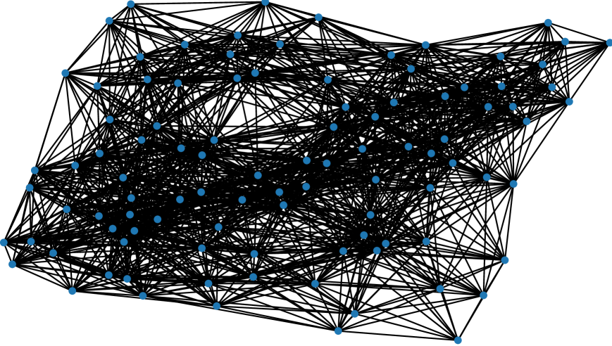
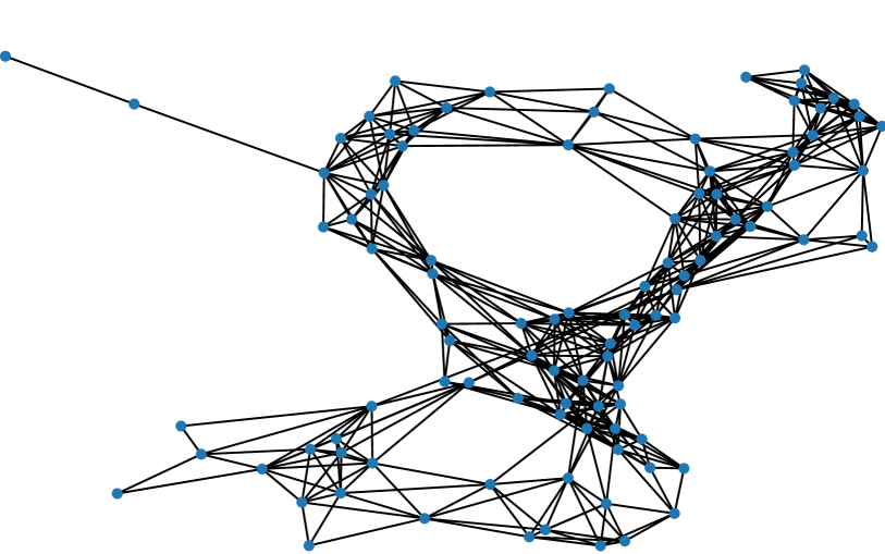
Figure 4: Random geometric networks used in synthetic data experiments, both with $N=100$: a dense network with an average degree of $31$ (left) and a sparse one with an average degree of $9.7$ (right).

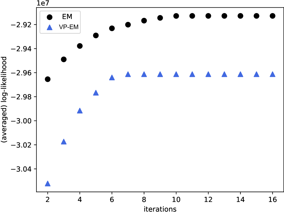
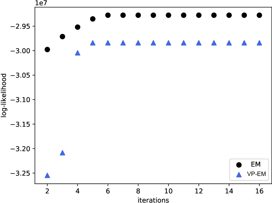
Figure 5: Log-likelihood trajectories for the synthetic data experiments: averaged per iteration over 5 runs on dense graphs (left); and run on sparse graph (right).

Synthetic data.

We illustrate the scalability of VP-EM on five random geometric networks with $N=100$, each fed $M=150,000$ examples sampled from a ground truth GMM with $K=3$ components created at random. The five setups differ in the network instance, data, and initializations, yet these networks have the same $N$ and similar density of connections (ratio between the number of network links and the number of links in a complete network, $\lvert\mathcal{E}\rvert/(N(N-1)/2)$). On the left sides of Figure 4 and Figure 5, respectively, we have one of the 5 networks and the evolution of $\mathcal{LL}$ averaged over the five runs, for both (centralized) EM and VP-EM. The simulations show $\mathcal{LL}$ increasing monotonically before plateauing, for both EM and our algorithm. VP-EM plateaus at a lower value, as expected, due to using block-diagonal matrices $\Sigma_{k}$ which make our algorithm less expressive than the centralized EM, which allows for fully dense matrices $\Sigma_{k}$.

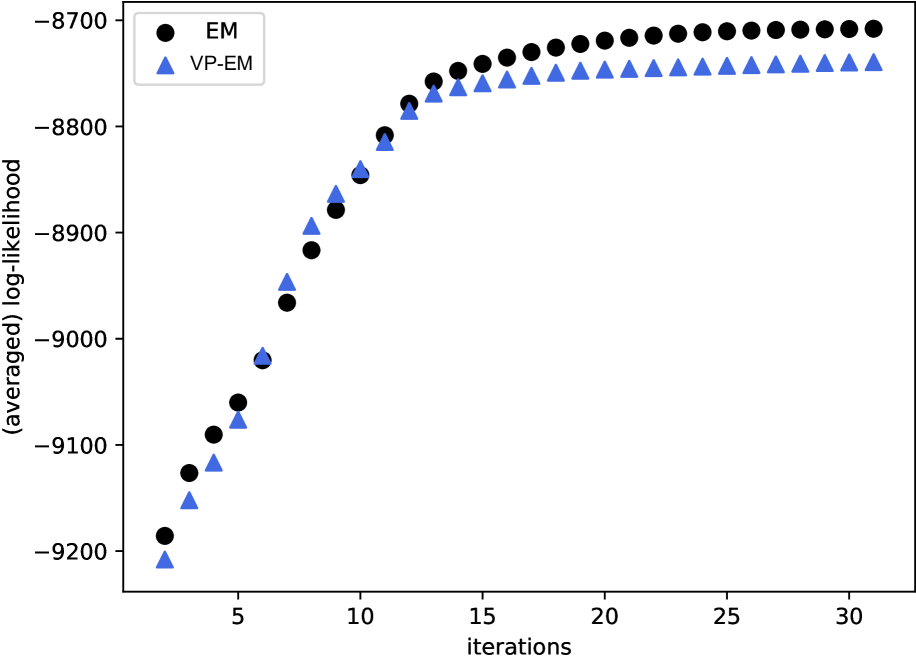
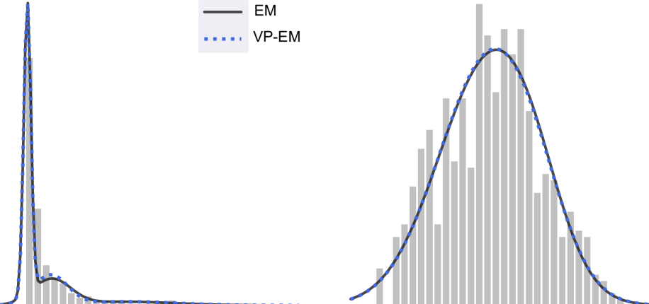
Figure 6: Log-likelihood trajectories for the real data experiment averaged per iteration over 5 runs (left). Marginal distributions of the EM and VP-EM GMMs superimposed on histograms of two features (right).

In Figure 4, on the right, we present the network used in an additional run of the algorithm, with the same $K$, $N$, and $T$ as before, but running VP-EM on a sparser network. As seen in Figure 5, on the right, we again observe a gap between the likelihoods attained by our algorithm and EM, due to the block-diagonal restriction on $\Sigma_{k}$ by the former. Both $\mathcal{LL}_{\text{EM}}$ and $\mathcal{LL}_{\text{VP-EM}}$ remain monotonic increasing.

Real data.

We now test VP-EM on real data from a European public service queue system. The data consists of a pool of $T_{\text{pool}}=2,650$ examples, each with $N=5$ features: daytime, weekday, queue, number of people waiting, and the power transform (Yeo and Johnson, 2000) of the moving average waiting times for the relevant queue. We sample this pool five times at random to form five datasets with $T=630$. Each such dataset is then split by features across a cycle of $N=5$ agents, $\mathcal{E}=\left\{\{1,2\},\{2,3\},\{3,4\},\{4,5\},\{5,1\}\right\}$. We chose a cycle graph due to it being one of the most challenging topologies for information spreading. A different cycle graph can be seen in Figure 7.

We ran (centralized) EM and VP-EM for each of the five samples. The trajectory of $\mathcal{LL}$ (averaged over the five runs) is shown in Figure 6. Again, both algorithms converge monotonically and, again, the gap between the two asymptotic values of $\mathcal{LL}$ is due to the sparsity imposed on $\Sigma_{k}$ by VP-EM. (We ran a centralized EM with the block-diagonal structure and saw its $\mathcal{LL}$ trajectory match that of VP-EM. Omitted to avoid clutter.) Figure 6 also shows the GMMs fitted by the centralized EM and VP-EM superimposed on the histograms for two of the features. The approximation seems good, yet, when approximating densities with GMMs, increasing $K$ may narrow the gap between $\mathcal{LL}_{\text{VP-EM}}$ plateau and $\mathcal{LL}_{\text{EM}}$. Here, a meager $K=3$ components allowed for good results. Yet, apart from a poor convergence (which we can mitigate by starting the algorithm multiple times with different initializations and taking the best result), increasing $K$ should not lower $\mathcal{LL}$ and may in fact increase it.

7.2 Clustering

Real data.

For clustering, we do have a benchmark. Ding et al. (2016) performs $k$-means clustering in FL settings. Thus, we now drop synthetic data altogether to avoid biasing the results with the choice of ground truth, focusing on real data. More precisely, we resort to data concerning pulsar candidates (measurements which may or not correspond to pulsars). Pulsar discovery is an important task in astronomy and, since modern approaches produce millions of candidates, a multitude of machine learning approaches has emergenced (e.g. Morello et al., 2014; Lyon et al., 2016). We use the labeled data provided by Lyon et al. (2016) for clustering, containing $M=17,898$ examples with $d=8$ features and the correct label. To facilitate running the experiments, we upper bound the performance of the distributed $k$-means clustering with the standard, centralized $k$-means. Since the dataset used was originally centralized, it has no communication graph associated with it, so we resort to synthetic networks. (While VP-EM can run on fully decentralized setups, if we were to run the benchmark, instead of the centralized $k$-means, it would require an FL scheme.) More precisely, we run VP-EM on three networks, as presented in Figure 7: a cycle graph (setup VP₁), a geometric graph (setup VP₂), and a scale-free graph (setup VP₃). In Table 1, we see that the (centralized) $k$-means is outperformed both by EM and by VP-EM, in all setups. We actually even outperform the centralized EM, which may be due to overfitting by the centralized EM, which imposes no sparsity on $\Sigma_{k}$.

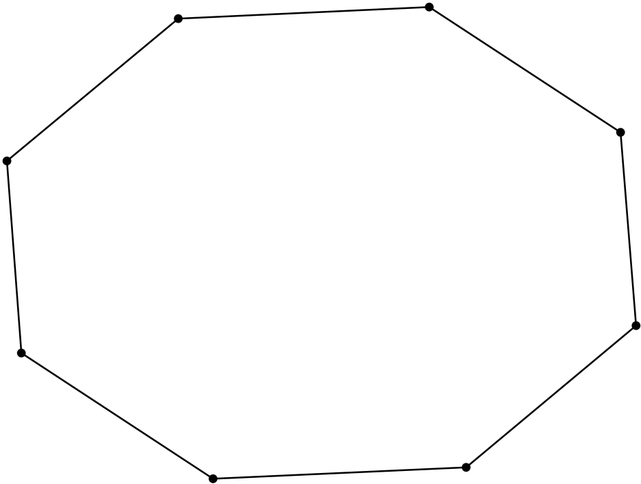
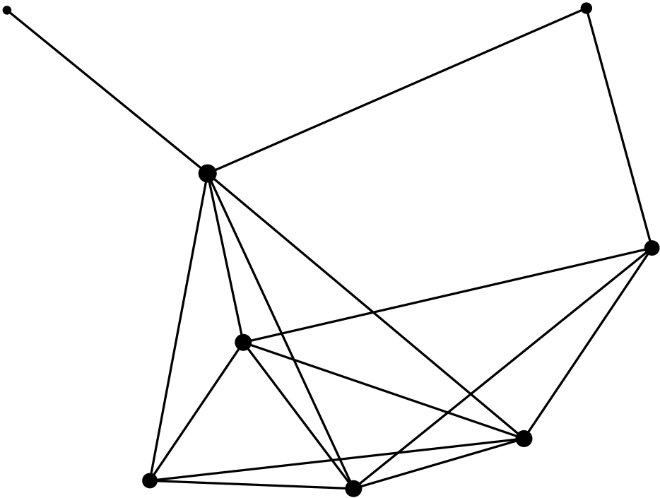
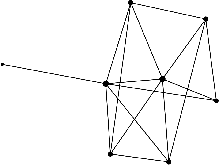
Figure 7: Cycle graph of VP₁ (left), geometric graph of VP₂ (middle), and scale-free graph of VP₃ (right). VP₂ and VP₃ have average degree 4.

Table 1: Clustering Accuracy

	$k$-means	EM	VP1	VP2	VP3
Acc.(%)	76.7	84.3	85.7	84.4	87.2

8 Discussion

We formulate the task of fitting GMMs to data distributed by features and identify its challenges. We propose an algorithm that copes with these challenges, both in FL and in fully decentralized setups, by partitioning parameters and constraining their space. As VP-EM generalizes from FL to fully decentralized schemes, we lose the monotonicity guarantee of the classic EM, but get an opportunity to exploit flexible graph topologies, allowing for a range of data sharing options which can relax the constraint on the parameter space. We demonstrate VP-EM on fully decentralized setups, using a large number of consensus rounds. In the future, it would be interesting to study the algorithm in communication-critical setups. Our results show that, in addition to outperforming the benchmark, VP-EM approximates well the centralized EM for both density estimation and clustering.

References

- Altilio et al. (2019) R. Altilio, P. D. Lorenzo, and M. Panella. Distributed data clustering over networks. Pattern Recognition, 93:603–620, 2019.
- Balakrishnan et al. (2014) S. Balakrishnan, M. J. Wainwright, and B. Yu. Statistical guarantees for the EM algorithm: From population to sample-based analysis, 2014.
- Bhaduri and Srivastava (2009) K. Bhaduri and A. N. Srivastava. A local scalable distributed expectation maximization algorithm for large peer-to-peer networks. In 2009 Ninth IEEE International Conference on Data Mining, pages 31–40, 2009.
- Bishop (2006) C. M. Bishop. Pattern Recognition and Machine Learning. Springer, 2006.
- Blei et al. (2003) D. M. Blei, A. Y. Ng, and M. I. Jordan. Latent dirichlet allocation. Journal of Machine Learning Research, 3:993–1022, 2003.
- Boyd et al. (2011) S. Boyd, N. Parikh, E. Chu, B. Peleato, and J. Eckstein. Distributed optimization and statistical learning via the alternating direction method of multipliers. Foundations and Trends in Machine Learning, 3:1–122, 2011.
- Chung (1994) F. Chung. Spectral graph theory. CBMS Regional Conference Series in Mathematics, 1994.
- Daskalakis et al. (2017) C. Daskalakis, C. Tzamos, and M. Zampetakis. Ten steps of EM suffice for mixtures of two Gaussians, 2017.
- Dedecius and Djurić (2017) K. Dedecius and P. M. Djurić. Sequential estimation and diffusion of information over networks: a Bayesian approach with exponential family of distributions. IEEE Transactions on Signal Processing, 65(7):1795–1809, 2017.
- Dempster et al. (1977) A. Dempster, N. Laird, and D. Rubin. Maximum likelihood from incomplete data via the EM algorithm. Royal Statistical Society, 39(1):1–22, 1977.
- Ding et al. (2016) H. Ding, Y. Liu, L. Huang, and J. Li. -means clustering with distributed dimensions. In M. F. Balcan and K. Q. Weinberger, editors, Proceedings of The 33rd International Conference on Machine Learning, volume 48 of Proceedings of Machine Learning Research, pages 1339–1348. PMLR, 2016.
- Duchi et al. (2012) J. C. Duchi, A. Agarwal, and M. J. Wainwright. Dual averaging for distributed optimization: Convergence analysis and network scaling. IEEE Transactions on Automatic Control, 57(3):592–606, 2012.
- Dwork (2008) C. Dwork. Differential privacy: A survey of results. In M. Agrawal, D. Du, Z. Duan, and A. Li, editors, Theory and Applications of Models of Computation, pages 1–19. Springer Berlin Heidelberg, 2008.
- Fagnani et al. (2013) F. Fagnani, S. M. Fosson, and C. Ravazzi. Consensus-like algorithms for estimation of Gaussian mixtures over large scale networks. Mathematical Models and Methods in Applied Sciences, 24(2):381–404, 2013.
- Forero et al. (2008) P. A. Forero, A. Cano, and G. B. Giannakis. Consensus-based distributed expectation-maximization algorithm for density estimation and classification using wireless sensor networks. In 2008 IEEE International Conference on Acoustics, Speech and Signal Processing, pages 1989–1992. IEEE, 2008.
- Forero et al. (2010) P. A. Forero, A. Cano, and G. B. Giannakis. Consensus-based distributed support vector machines. Journal of Machine Learning Research, 11(55):1663–1707, 2010.
- Ghahramani and Jordan (1993) Z. Ghahramani and M. I. Jordan. Supervised learning from incomplete data via an em approach. In Proceedings of the 6th International Conference on Neural Information Processing Systems, NIPS’93, page 120–127. Morgan Kaufmann Publishers Inc., 1993.
- Grozavu and Bennani (2010) N. Grozavu and Y. Bennani. Topological collaborative clustering. Australian Journal of Intelligent Information Processing Systems, 12(3), 2010.
- Gu (2008) D. Gu. Distributed em algorithm for Gaussian mixtures in sensor networks. IEEE Transactions on Neural Networks, 19:1154–1166, 2008.
- Hu et al. (2007) Y. Hu, H. Chen, J.-g. Lou, and J. Li. Distributed density estimation using non-parametric statistics. In 27th International Conference on Distributed Computing Systems (ICDCS’07). IEEE, 2007.
- Hua and Li (2015) J. Hua and C. Li. Distributed variational bayesian algorithms over sensor networks. IEEE Transactions on Signal Processing, 64(3):783–798, 2015.
- Kairouz et al. (2021) P. Kairouz, H. B. McMahan, et al. Advances and open problems in federated learning, 2021.
- Kowalczyk and Vlassis (2005) W. Kowalczyk and N. Vlassis. Newscast EM. In L. Saul, Y. Weiss, and L. Bottou, editors, Advances in Neural Information Processing Systems, volume 17. MIT Press, 2005.
- Kunstner et al. (2021) F. Kunstner, R. Kumar, and M. W. Schmidt. Homeomorphic-invariance of EM: Non-asymptotic convergence in KL divergence for exponential families via mirror descent. In AISTATS, 2021.
- Li et al. (2012) C. Li, D. Porto, A. Clement, J. Gehrke, N. Preguiça, and R. Rodrigues. Making geo-replicated systems fast as possible, consistent when necessary. In 10th USENIX Symposium on Operating Systems Design and Implementation (OSDI 12), pages 265–278. USENIX Association, 2012.
- Lian et al. (2017) X. Lian, C. Zhang, H. Zhang, C.-J. Hsieh, W. Zhang, and J. Liu. Can decentralized algorithms outperform centralized algorithms? a case study for decentralized parallel stochastic gradient descent, 2017.
- Lyon et al. (2016) R. J. Lyon, B. W. Stappers, S. Cooper, J. M. Brooke, and J. D. Knowles. Fifty years of pulsar candidate selection: from simple filters to a new principled real-time classification approach. Monthly Notices of the Royal Astronomical Society, 459(1):1104–1123, Apr 2016.
- Mann et al. (2009) G. Mann, R. McDonald, M. Mohri, N. Silberman, and D. W. IV. Efficient large-scale distributed training of conditional maximum entropy models. In Neural Information Processing Systems (NIPS), 2009.
- McMahan et al. (2017) H. B. McMahan, E. Moore, D. Ramage, S. Hampson, and B. A. y Arcas. Communication-efficient learning of deep networks from decentralized data, 2017.
- Morello et al. (2014) V. Morello, E. D. Barr, M. Bailes, C. M. Flynn, E. F. Keane, and W. van Straten. SPINN: a straightforward machine learning solution to the pulsar candidate selection problem. Monthly Notices of the Royal Astronomical Society, 443(2):1651–1662, Jul 2014.
- Neal and Hinton (1993) R. M. Neal and G. E. Hinton. A new view of the EM algorithm that justifies incremental and other variants. In Learning in Graphical Models, pages 355–368. Kluwer Academic Publishers, 1993.
- Nedic and Ozdaglar (2009) A. Nedic and A. Ozdaglar. Distributed subgradient methods for multi-agent optimization. IEEE Transactions on Automatic Control, 54(1):48–61, 2009.
- Nedić and Ozdaglar (2010) A. Nedić and A. Ozdaglar. Cooperative distributed multi-agent optimization. In D. P. Palomar and Y. C. Eldar, editors, Convex Optimization in Signal Processing and Communications, pages 340–386. Cambridge University Press, 2010.
- Nowak (2003) R. Nowak. Distributed EM algorithms for density estimation and clustering in sensor networks. IEEE Transactions on Signal Processing, 51(8):2245–2253, 2003.
- Olshevsky and Tsitsiklis (2009) A. Olshevsky and J. N. Tsitsiklis. Convergence speed in distributed consensus and averaging. SIAM Journal on Control and Optimization, 48(1):33–55, 2009.
- Qu and Li (2018) G. Qu and N. Li. Harnessing smoothness to accelerate distributed optimization. IEEE Transactions on Control of Network Systems, 5(3):1245–1260, 2018.
- Rieke et al. (2020) N. Rieke, J. Hancox, W. Li, et al. The future of digital health with federated learning. npj Digital Medicine, 3(1), Sep 2020.
- Rivest et al. (1978) R. L. Rivest, L. Adleman, and M. L. Dertouzos. On data banks and privacy homomorphisms, 1978.
- Saber and Murray (2003) R. O. Saber and R. M. Murray. Consensus protocols for networks of dynamic agents. Proceedings of the 2003 American Control Conference, 2:951–956, 2003.
- Safarinejadian et al. (2010) B. Safarinejadian, M. B. Menhaj, and M. Karrari. A distributed EM algorithm to estimate the parameters of a finite mixture of components. Knowledge and Information Systems, 23(3):267–292, 2010.
- Schaeffer (2007) S. E. Schaeffer. Graph clustering. Computer Science Review, 1(1):27–64, 2007.
- Sorenson and Alspach (1971) H. W. Sorenson and D. L. Alspach. Recursive Bayesian estimation using Gaussian sums. Automatica, 7(4):465–479, 1971.
- Vaidya and Clifton (2003) J. Vaidya and C. Clifton. Privacy-preserving k-means clustering over vertically partitioned data. Proceedings of the ninth ACM SIGKDD international conference on Knowledge discovery and data mining, pages 206–215, 2003.
- Wang et al. (2019) K. Wang, R. Mathews, C. Kiddon, H. Eichner, F. Beaufays, and D. Ramage. Federated evaluation of on-device personalization, 2019.
- Weng et al. (2011) Y. Weng, W. Xiao, and L. Xie. Diffusion-based EM algorithm for distributed estimation of Gaussian mixtures in wireless sensor networks. Molecular Diversity Preservation International, 11:6297–6316, 2011.
- Wu (1983) C. F. J. Wu. On the convergence properties of the EM algorithm. The Annals of Statistics, 11(1):95–103, 1983.
- Xiao and Boyd (2004) L. Xiao and S. Boyd. Fast linear iterations for distributed averaging. Systems & Control Letters, 53:65–78, 2004.
- Xiao et al. (2005) L. Xiao, S. Boyd, and S. Lall. A scheme for robust distributed sensor fusion based on average consensus. In IPSN 2005. Fourth International Symposium on Information Processing in Sensor Networks, 2005., pages 63–70, 2005.
- Yang et al. (2019) Q. Yang, Y. Liu, T. Chen, and Y. Tong. Federated machine learning: Concept and applications, 2019.
- Yeo and Johnson (2000) I.-K. Yeo and R. A. Johnson. A new family of power transformations to improve normality or symmetry. Biometrika, 87(4):954–959, 2000.
- Ying et al. (2018) B. Ying, K. Yuan, and A. H. Sayed. Supervised learning under distributed features. IEEE Transactions on Signal Processing, 67:977–922, 2018.