Euclidean and Affine Curve Reconstruction

Abstract

We consider practical aspects of reconstructing planar curves with prescribed Euclidean or affine curvatures. These curvatures are invariant under the special Euclidean group and the special affine groups, respectively, and play an important role in computer vision and shape analysis. We discuss and implement algorithms for such reconstruction, and give estimates on how close reconstructed curves are relative to the closeness of their curvatures in appropriate metrics. Several illustrative examples are provided.

Jose Agudelo	Brooke Dippold	Ian Klein
University of New Mexico	Longwood University	NC State University
joseagudelo@unm.edu	brookedippold1@gmail.com	iklein@ncsu.edu
orcid: 0000-0001-5052-2112	orcid: 0000-0001-9274-6704	orcid:0000-0003-1140-226X
Alex Kokot	Eric Geiger	Irina Kogan
University of Washington	Yale University	NC State University
akokot@uw.edu	eric.geiger@yale.edu	iakogan@ncsu.edu
orcid: 0000-0001-6163-6051	orcid:0000-0002-5296-0199	orcid: 0000-0001-8212-6296

Keywords: Planar curves; Euclidean and affine transformations; Euclidean and affine curvatures; Curve reconstruction; Picard iterations; Distances.

MSC: 53A04, 53A15, 53A55, 34A45, 68T45.

1 Introduction

Rigid motions – compositions of translation, rotations and reflections – are fundamental transformations on the plane studied in a high-school geometry course. Two shapes related by these transformations are called congruent. The geometry studied in high-school is based on the set of axioms formulated by Euclid about 300BC and is called the Euclidean geometry. Rigid motions comprise the set of all transformations on the plane that preserve Euclidean distance between two points. A composition of two rigid motions is again a rigid motion, and the set of all rigid motions with the binary operation defined by composition satisfies the definition of a group (see Section 2.1). Naturally, this group is called the Euclidean group and is denoted by $E(2)$, where $2$ indicates that the motions are considered in the 2-dimensional space, the plane.

To a human eye, two figures look the same if they are related by a rigid motion. However, since a reflection changes the orientation of an object, a group of orientation-preserving rigid motions, consisting of rotations and translations only, is often considered. This group is called the special Euclidean group and is denoted by $SE(2)$. In many applications, the congruence with respect to other groups is considered. For example, two shadows cast by the same object onto two different planes by blocking the rays of light emitted from a lamp are related by a projective transformation. If a light source can be considered to be infinitely far away (like a sun), then the shadows are related by an affine transformation. See [13] for an excellent exposition of the roles played by projective, (special) affine, and (special) Euclidean transformations in computer vision. Staring in the 19th century, it was widely accepted that Euclidean geometry, although the most intuitive, is not the only possible consistent geometry, and that congruence can be defined relative to other transformations groups [14].

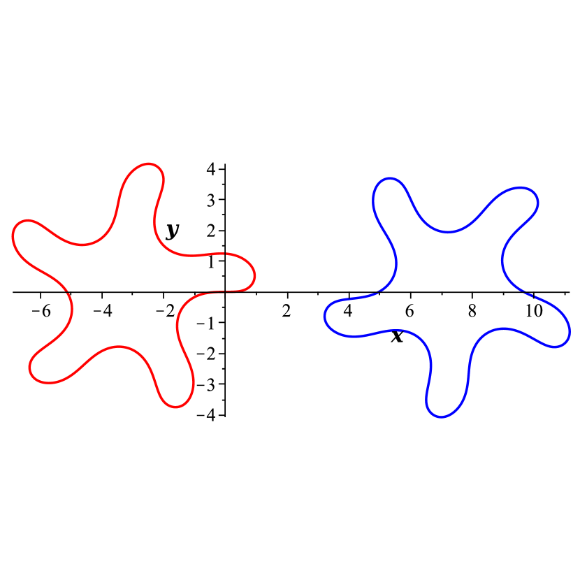
Figure 1: A special Euclidean transformation is a composition of a rotation and a translation.

Figure 2: A special affine transformation is a composition of a unimodular linear transformation and a translation.

In this work, we consider congruence of planar curves relative to the special Euclidean group $SE(2)$ and the special affine group $SA(2)$. The latter group consists of compositions of area and orientation preserving (i.e. unimodular) linear transformations and translations, and is sometimes also called the equi-affine group. In Figure 2, we show two curves related by a special Euclidean transformation, while in Figure 2 we show two curves related by a special affine transformation. For applications of curve matching under (special) Euclidean and affine transformations see, for instance, [24, 4, 3, 1, 9, 10, 7, 15].

It is widely known that two sufficiently smooth planar curves are $SE(2)$-congruent if they have the same Euclidean curvature $\kappa$ as a function of the Euclidean arc-length $s$. Somewhat less familiar, but also known from 19th century, are the notions of curvature and arc-length in other geometries, in particular in the special affine geometry, [12]. Similarly to the Euclidean case, one can show that two sufficiently smooth planar curves are $SA(2)$-congruent if they have the same affine curvature $\mu$ as a function of the affine arc-length $\alpha$. Knowing that the curvature as a function of the arc-length determines a curve up to the relevant group of transformations, it is natural to ask two questions:

1. Is there a practical algorithm to reconstruct a curve from its curvature up to the relevant transformation group?

2. If two curvatures are close to each other in a certain metric, how close can the reconstructed curves be brought to each other by an element of the relevant transformation group?

In this paper, we study both of these questions, by methods and techniques that are well known. Namely, we review and implement a procedure for reconstructing a curve from its Euclidean curvature by successive integrations. The procedure for reconstructing curves from its affine curvature is more complicated and is based on Picard iterations. An implementation of these procedures can be found at https://egeig.com/research/curve_reconstruction. In Theorem 12, we show how close, relative to the Hausdorff metric, two curves can be brought together by a special Euclidean transformation if their Euclidean curvatures are $\delta$-close in $L^{\infty}$-norm. Theorem 19 addresses the same question in the special affine case.

Many of the theoretical results presented in this paper are well known and the new results presented here are hardly surprising. However, combined together and illustrated by specific examples, we believe, they contribute to a better understanding of a classical, but important problem, relevant in many modern applications. This paper is a result of an REU project, which turned out to be of a great pedagogical value, as it taught the students to combine the results and methods from various subjects: differential geometry, algebra, analysis and numerical analysis. In addition, this project involved theoretical work and the work of designing and implementing algorithms. The multidisciplinary nature of this project, on one hand, and its accessibility, on the other hand, allowed the undergraduate participants to truly experience the richness and challenges of mathematical research. We hope that we are able to convey to the reader the enjoyment of various aspects of the mathematical research that we experienced while working on the project.

The paper is structured as follows. Section 2 contains preliminaries and is split in the following subsections. In Section 2.1, we review the definitions of groups and group actions and then define the notion of congruence and symmetry of curves relative to a given group. In Sections 2.2 and 2.3, we follow [12] to define Euclidean and affine moving frames and invariants. In Section 2.4, we introduce norms and distances in the spaces of functions, matrices, matrices of functions, and curves that are used in this paper and establish some useful inequalities. In Section 2.5, we establish some results about convergence of matrices and their norms.

Section 3 contains explicit formulas for reconstructing a curve from its Euclidean curvature function and gives an upper bound on the closeness of reconstructed curves with close Euclidean curvatures. Section 4 introduces a Picard iteration scheme for reconstructing a curve from its affine curvature function and gives an upper bound on the closeness of reconstructed curves with close affine curvatures. Directions of further research are indicated in Section 5. In the appendix, we derive power series for curves whose affine curvatures are given by a monomial.

2 Preliminaries

2.1 Congruence and symmetry of the planar curves

To keep the presentation self-contained, we remind the reader the standard definitions of groups and group-actions.

Definition 1.

A group is a set $G$ with a binary operation $``\cdot"\colon G\times G\to G$ that satisfies the following properties:

1. Associativity: $(g_{1}\cdot g_{2})\cdot g_{3}=g_{1}\cdot(g_{2}\cdot g_{3})$, $\forall g_{1},g_{2},g_{3}\in G.$

2. Identity element: There exists a unique $e\in G$, such that $e\cdot g=g\cdot e=g$, $\forall g\in G$.

3. Inverse element: For each $g\in G$, there exists an element $h\in G$ such that $g\cdot h=h\cdot g=e$. We denote $g^{-1}:=h.$

Definition 2.

An action of a group $G$ on a set $P$ is a map $\phi\colon G\times P\to P$ satisfying the following properties:

1. Associativity: $\phi(g_{1}\cdot g_{2},p)=\phi(g_{1},\phi(g_{2},p))$, $\forall g_{1},g_{2}\in G$ and $\forall p\in P$

2. Action of the identity element: $\phi(e,p)=p$, $\forall p\in P$.

We denote $\phi(g,p):=gp$. Each element $g\in G$ determines a bijective map $g\colon P\to P$, $p\to gp$.

Groups are often defined through their actions. For example, a rotation in the plane by angle $\theta>0$ about the origin in the counter-clockwise direction sends a point $(x,y)$ in the plane to a point

$$(\bar{x},\bar{y})=(x\cos\theta-y\sin\theta,x\sin\theta+y\cos\theta)=(x,y)R_{\theta}^{-1},$$ (1)

where the $2\times 2$ matrix $R_{\theta}$ is given by

$$R_{\theta}=\begin{pmatrix}\cos\theta&-\sin\theta\\ \sin\theta&\cos\theta\end{pmatrix}.$$ (2)

We multiply by the matrix on the right because we treat points (and vectors) in $\mathbb{R}^{2}$ as row vectors. We invert the matrix to satisfy the associativity property in the definition of the group action . Rotation by $\theta=0$ corresponds to the identity matrix and leaves all points in place, while $R_{\theta}$ with $\theta<0$ corresponds to the clockwise rotation by angle $|\theta|$. The set of matrices $\{R_{\theta}\,|\,\theta\in\mathbb{R}\}$ with the binary operation given by matrix multiplication satisfies the definition of a group. This group is called the special orthogonal group and is denoted by $SO(2)$. The word special in the name of the group indicates that $\det(R_{\theta})=1$ and so the orthonormal bases defined by its columns (or rows) is positively oriented. In fact, the group $SO(2)$ consists of all $2\times 2$ matrices whose two columns (or two rows) form a positively oriented orthonormal basis in $\mathbb{R}^{2}$. The map $\phi\colon SO(2)\times\mathbb{R}^{2}\to\mathbb{R}^{2}$defined by (1) satisfies the definition of a group-action. The associativity property in Definition 2 states that the action of the product of matrices $R_{\theta_{1}}\cdot R_{\theta_{2}}$ is the composition of the rotation by angle $\theta_{2}$ followed by rotation by angle $\theta_{1}$.

The translation in the plane by a vector ${\bf v}=(a,b)$ sends a point $(x,y)$ to a point

$$(\bar{x},\bar{y})=(x,y)+(a,b)=(x+a,y+b).$$ (3)

The set of vectors ${\bf v}\in\mathbb{R}^{2}$ with the binary operation given by vector addition satisfies the definition of a group, with the zero vector being the identity element of this group. Formula (3) describes the action of this group on the plane. A composition of a rotation by $\theta$ followed by a translation by ${\bf v}$ sends a point $(x,y)$

$$(\bar{x},\bar{y})=(x\cos\theta-y\sin\theta+a,x\sin\theta+y\cos\theta+b)=(x,y)R_{\theta}^{-1}+{\bf v}.$$ (4)

The set of all compositions of rotations and translations also satisfies the definition of the group. It is called the special Euclidean group and is denoted $SE(2)$. This is the group of all transformations in the plane that preserves distances (and, therefore, angles) in the plane, as well as the orientation. A composition of a rotation/translation pair $(R_{\theta_{2}},{\bf v}_{2})$ followed by a pair $(R_{\theta_{1}},{\bf v}_{1})$ is equivalent to rotation $R_{\theta_{1}}R_{\theta_{2}}=R_{\theta_{1}+\theta_{2}}$ followed by a translation by the vector ${\bf v}_{2}R_{\theta_{1}}^{-1}+{\bf v}_{1}$. Thus we can think of the special Euclidean group as the set of pairs $\{(R_{\theta},{\bf v})\,|\,R_{\theta}\in SO(2),{\bf v}\in\mathbb{R}^{2}\}$ with the group operation

$$(R_{\theta_{1}},{\bf v}_{1})\cdot(R_{\theta_{2}},{\bf v}_{2})=\left(R_{\theta_{1}}R_{\theta_{2}},{\bf v}_{2}R_{\theta_{1}}^{-1}+{\bf v}_{1}\right).$$ (5)

In other words, $SE(2)=SO(2)\ltimes\mathbb{R}^{2}$ is a semi-direct product of the translation and rotation groups.

If in (4) and (5), we replace the rotation matrix $R_{\theta}$ with an arbitrary non-singular $2\times 2$ matrix $M$, we obtain an action of the affine group, $A(2)=GL(2)\ltimes\mathbb{R}^{2}$, a semi-direct product of the group of invertible linear transformations and translations. Restricting the matrix $M$ to the group of unimodular matrices $SL(2)=\{M\,|\,\det(M)=1\}$, we obtain a smaller group which is called the special affine or the equi-affine group $SA(2)=SL(2)\ltimes\mathbb{R}^{2}$. A generic $SA(2)$-transformation does not preserve distance or angles, but it preserves areas.

An action of a group on the plane induces the action on the curves in the plane. In this paper, we consider curves satisfying the following definition.

Definition 3 (Planar curve).

A planar curve $\mathcal{C}$ is the image of a continuous locally injective map $\gamma\colon\mathbb{R}\to\mathbb{R}^{2}$. We call $\mathcal{C}$ closed if its parameterization $\gamma$ is periodic. We often restrict the domain of $\gamma$ to an open or a closed interval $I\subset\mathbb{R}$.

If, in the subset topology, $\gamma(I)$ is homeomorphic to $I$, we call the image an open (or a closed) curve segment. If, in the subset topology, $\gamma(I)$ is homeomorphic to a circle, we call the image a loop. Curve segments and loops that do not have points of self-intersections are called simple curves. Given a group $G$ acting continuously on the plane, the image of a curve $\mathcal{C}$ parametrized by $\gamma$, under a transformation $g\in G$ is the curve $g\mathcal{C}=\{gp\,|\,p\in\mathcal{C}\}$ parametrized by $g\gamma=g\circ\gamma$.

Definition 4.

Given a group $G$ acting on the plane, we say that two planar curves $\mathcal{C}_{1}$ and $\mathcal{C}_{2}$ are called G-congruent ($\mathcal{C}_{1}\underset{G}{\cong}\mathcal{C}_{2}$) if there exists $g\in G$, such that $\mathcal{C}_{2}=g\,\mathcal{C}_{1}$.

Definition 5.

An element $g\in G$ is a $G$-symmetry of $\mathcal{C}$ if

$$g\,\mathcal{C}=\mathcal{C}.$$

It easy to show that the set of such elements, denoted $\text{sym}_{G}(\mathcal{C})$, is a subgroup of $G$, called the $G$-symmetry group of $\mathcal{C}$. The cardinality of $\text{sym}_{G}(\mathcal{C})$ is called the symmetry index of $\mathcal{C}$.

In Figure 2, we show two $SE(2)$-congruent curves, each with five $SE(2)$-symmetries. In Figure 2, we show two $SA(2)$-congruent curves, each with five $SA(2)$-symmetries. As a side remark, we note that the five $SA(2)$-symmetries of the left curve in Figure 2, in fact, belong to $SE(2)$, while the five $SA(2)$-symmetries of the right curve do not. The method of moving frames, pioneered by Bartels, Frenet, Serret, Cotton, and Darboux, and greatly extended by Cartan, allows to solve the $G$-congruence problem for sufficiently smooth curves by assigning a frame of basis vectors along a curve, in a way that is compatible with the $G$-action. We will review this classical construction of such frames for the $SE(2)$ and $SA(2)$ actions by following, for the most part, the exposition given in [12]. For a more detailed history and generalizations to arbitrary Lie group-actions see [16].

2.2 Euclidean moving frame and invariants

The $SE(2)$-frame at point $p$ of a planar curve $\mathcal{C}$ consists of the unit tangent vector $T(p)$ and the unit normal vector $N(p)$. Orientation for $T(p)$ is defined by the parameterization $\gamma$ of $\mathcal{C}$, while the orientation for $N(p)$ is chosen so that the pair of vectors $T(p)$ and $N(p)$ is positively oriented, i.e. the closest rotation from $T(p)$ to $N(p)$ is counter-clockwise. Considering $T$ and $N$ to be row vectors, we combine them into an $SE(2)$-frame matrix

$$A_{\mathcal{C}}(p)=\begin{pmatrix}{}T(p)\\ N(p)\\ \end{pmatrix}.$$ (6)

An important observation is that $A_{\mathcal{C}}(p)$ is an orthogonal matrix. In fact, it is precisely the rotation matrix which brings the moving frame basis consisting of $T(p)$ and $N(p)$ to the standard orthonormal basis in $\mathbb{R}^{2}$ under the action (1). An element $g\in SE(2)$ acting on $\mathbb{R}^{2}$ maps the curve $\mathcal{C}$ to $\tilde{\mathcal{C}}$ and the point $p$ to $\tilde{p}$. Since the $SE(2)$-action preserves tangency and length, it maps the $SE(2)$-frame at $p\in\mathcal{C}$ to the $SE(2)$-frame at $\tilde{p}\in\tilde{\mathcal{C}}$. See Figure 4 for an illustration. This compatibility property of the frame is called equivariance and can be expressed as

$$A_{g\,\mathcal{C}}(gp)=A_{\mathcal{C}}(p)R_{g}^{-1},$$ (7)

where $\mathcal{C}$ is an arbitrary curve, $p\in\mathcal{C}$, $g\in SE(2)$, $R_{g}$ is the rotational part of the transformation $g$.

It is well known that any $C^{1}$-smooth non-degenerate curve $\mathcal{C}$ can be parametrized

$$\gamma\colon s\to p=\gamma(s),$$

so that

$$T(s)=\gamma_{s}(s)$$ (8)

is the unit tangent vector at the point $\gamma(s)\in\mathcal{C}$. (Here and below, a variable in the subscript denotes the differentiation with respect to this variable). Explicitly, if $\hat{\gamma}\colon t\to\gamma(t)=(x(t),y(t))$ is any parametrization of $\mathcal{C}$, then

$$s(t)=\int_{0}^{t}|\hat{\gamma}_{\tau}|d\tau=\int_{0}^{t}\sqrt{x^{\prime}(\tau)^{2}+y^{\prime}(\tau)^{2}}d\tau.$$

The parameter $s$ is called the Euclidean arc-length parameter. Its differential

$$ds=|\hat{\gamma}_{t}|dt$$ (9)

is called the infinitesimal Euclidean arc-length. Clearly, the integral of $ds$ along a curve segment produces the Euclidean length of the curve-segment.

We now assume that $\mathcal{C}$ is $C^{2}$-smooth and note that the differentiation of the identity $|T(s)|=1$ implies that $T_{s}(s)$ is orthogonal to $T(s)$, and so $T_{s}(s)$ is proportional to $N(s)$. Thus there is a function $\kappa(s)$, called the Euclidean curvature function, such that

$$T_{s}(s)=\kappa(s)N(s).$$ (10)

Explicitly, $\kappa(s)=\pm|\gamma_{ss}|$, with $``+"$ when the rotation from $\gamma_{s}$ to $\gamma_{ss}$ is counterclockwise and $``-"$ otherwise. For an arbitrary parameterization $\hat{\gamma}(t)$, we have

$$\kappa(t)=\frac{\det(\hat{\gamma}_{t},\hat{\gamma}_{tt})}{|\hat{\gamma}_{t}|^{3}}.$$ (11)

The Euclidean curvature of a circle of radius $r$ is constant and is equal to $\frac{1}{r}$. The Euclidean curvature of $\mathcal{C}$ at $p$ equals the curvature of its osculating circle at $p$.

Since $|N(s)|=1$, then $N_{s}(s)$ is proportional to $T(s)$. Furthermore, differentiating the scalar product identity $T(s)\cdot N(s)=0$, we conclude:

$$N_{s}(s)=-\kappa(s)T(s).$$ (12)

Equations (10) and (12) are called Frenet equations and can be written in the matrix form as

$$A_{s}=CA,$$

where $A$ is the Euclidean frame matrix (6), while

$$C(s)=A_{s}(s)A(s)^{-1}=\begin{pmatrix}0&\kappa(s)\\ -\kappa(s)&0\end{pmatrix}$$ (13)

is the Euclidean Cartan matrix. From the equivariance property (7), the $SE(2)$-invariance of $C$ and, therefore, of $\kappa$ follows:

$$\kappa_{g\mathcal{C}}(gp)=\kappa_{\mathcal{C}}(p),$$

where $\mathcal{C}$ is an arbitrary curve, $p\in\mathcal{C}$, $g\in SE(2)$.

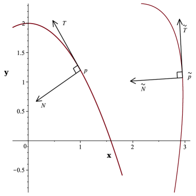
Figure 3: The $SE(2)$-action preserves the lengths of vectors and the angle between them.

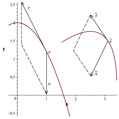
Figure 4: The $SA(2)$-action preserves the area of the parallelogram defined by the affine tangent and normal vectors, but not their lengths or the angle between them.

2.3 Affine moving frame and invariants

The action of the special affine group $SA(2)$ preserves neither Euclidean distances nor angles. Thus the Euclidean moving frame consisting of the unit tangent and the unit normal at each point of a curve $\mathcal{C}$ is not compatible with the $SA(2)$-action. However, the $SA(2)$-action preserves areas, and we can use this property to define an $SA(2)$-equivariant frame.

It turns out that any $C^{2}$-smooth curve $\mathcal{C}$ can be parametrized by

$$\gamma\colon\alpha\to p=\gamma(\alpha),$$

so that the area of the parallelogram defined by vectors

$$T(p)=\gamma_{\alpha}\text{ and }N(p)=\gamma_{\alpha\alpha}$$ (14)

is 1 and the closest rotation from $T(p)$ to $N(p)$ is counter-clockwise. The parameter $\alpha$ is called the affine arc-length parameter. Explicitly, if $\hat{\gamma}\colon t\to\gamma(t)=(x(t),y(t))$ is any parametrization of $\mathcal{C}$, then

$$\alpha(t)=\int_{0}^{t}\det(\hat{\gamma}_{\tau}(\tau),\hat{\gamma}_{\tau\tau}(\tau))^{1/3}d\tau.$$ (15)

Recalling formulas (9) and (11), we rewrite (15) in term of the Euclidean curvature and arc-length:

$$\alpha(s)=\int_{0}^{s}\kappa(\tau)^{1/3}d\tau.$$ (16)

Vectors $T(p)=\gamma_{\alpha}$ and $N(p)=\gamma_{\alpha\alpha}$ are called the affine tangent and normal to ${\mathcal{C}}$ at $p$, respectively. It is important to note that although $T(p)$ is tangent to ${\mathcal{C}}$ at $p$, it is, in general, not of the unit length, while $N(p)$, in general, is neither perpendicular to $T(p)$ nor of the unit length. The $SA(2)$-frame matrix is then defined by

$$A_{\mathcal{C}}(p)=\begin{pmatrix}T(p)\\ N(p)\end{pmatrix}=\begin{pmatrix}\gamma_{\alpha}\\ \gamma_{\alpha\alpha}\\ \end{pmatrix}.$$ (17)

An important observation is that, by construction, $\det(A_{\mathcal{C}}(p))=1$. In fact, this is the matrix of the unimodular linear transformation which brings the affine moving frame basis consisting of $T(p)$ and $N(p)$ to the standard orthonormal basis under the action on row vectors ${\bf v}\to{\bf v}M^{-1}$.

The affine moving frame is $SA(2)$-equivariant: an element $g\in SA(2)$ mapping the curve $\mathcal{C}$ to $\tilde{\mathcal{C}}$ and the point $p\in\mathcal{C}$ to the point $\tilde{p}\in\tilde{\mathcal{C}}$, also maps the affine tangent and normal at $p\in\mathcal{C}$ to the affine tangent and normal vectors $\tilde{p}\in\tilde{\mathcal{C}}$. See Figure 4 for an illustration. In the matrix form, this can be expressed as

$$A_{g\,\mathcal{C}}(gp)=A_{\mathcal{C}}(p)M_{g}^{-1},$$ (18)

where $\mathcal{C}$ is an arbitrary curve, $p\in\mathcal{C}$, $g\in SA(2)$, and $M_{g}$ is the matrix part of $g$.

By definition:

$$T_{\alpha}(\alpha)=N(\alpha).$$ (19)

Using this and differentiating the identity $\det(T(\alpha),N(\alpha))=1$ with respect to $\alpha$ we obtain $\det(T(\alpha),N_{\alpha}(\alpha))=0$. This implies that $N_{\alpha}$ is proportional to $T$, and, therefore, there is a function $\mu(\alpha)$, called the affine curvature function, such that

$$N_{\alpha}(\alpha)=-\mu(\alpha)T(\alpha),$$ (20)

where

$$\mu(\alpha)=-\det(N_{\alpha}(\alpha),N(\alpha))=\det(\gamma_{\alpha\alpha}(\alpha),\gamma_{\alpha\alpha\alpha}(\alpha)).$$ (21)

If $\hat{\gamma}(t)$ is an arbitrary parameterization of $\mathcal{C}$, then the formula for $\mu(t)$ is rather long (see formula (7-24) in [12]), but we can get a more concise formula in terms of the Euclidean curvature and the Euclidean arc-length [17]:

$$\mu=\frac{3\kappa(\kappa_{ss}+3\kappa^{3})-5\kappa_{s}^{2}}{9\kappa^{8/3}}.$$ (22)

The affine curvature of a conic is constant (see Section 4 for the details). The affine curvature of $\mathcal{C}$ at $p$ is the curvature of the osculating conic at $p$.

Equations (19) and (20) are the affine version of the Frenet equations and can be written in the matrix form as

$$A_{\alpha}(\alpha)=C(\alpha)A(\alpha),$$ (23)

where $A$ is the affine frame matrix (17), while

$$C(\alpha)=A_{\alpha}(\alpha)A(\alpha)^{-1}=\begin{pmatrix}0&1\\ -\mu(\alpha)&0\end{pmatrix}$$ (24)

is the affine Cartan matrix. From the equivariance property (18), the $SA(2)$-invariance of $C$ and, therefore, of $\mu$ follows:

$$\mu_{g\mathcal{C}}(gp)=\mu_{\mathcal{C}}(p),$$

where $\mathcal{C}$ is an arbitrary curve, $p\in\mathcal{C}$, and $g\in SA(2)$.

2.4 Norms and distances

For a continuous function $f(t)$ on a closed interval $[0,L]$, let

$$\left|\left|f\right|\right|_{[0,L]}:=\max_{t\in[0,L]}\{|f(t)|\}.$$ (25)

For a $k\times\ell$ matrix $A$ with real entries we define:

$$\left<A\right>:=\max_{{i=1,\dots,k}\atop{j=1,\dots,\ell}}\{|a_{ij}|\},$$ (26)

where $a_{ij}$ are the entries of $A$ and $|\cdot|$ is the usual absolute value. If $A(t)$ is a matrix whose entries are functions on a real interval $[0,L]$, we define a real valued function

$$\left<A\right>(t):=\left<A(t)\right>.$$ (27)

If the entries of $A(t)$ are continuous functions, it is easy to show that $\left<A\right>(t)$ is continuous on the interval $[0,L]$ and so we may define:

$$\left|\left|A\right|\right|_{[0,L]}:=\left|\left|\left<A\right>(t)\right|\right|_{[0,L]}=\max_{t\in[0,L]}\left<A(t)\right>=\max_{{t\in[0,L]}\atop{{i=1,\dots,k}\atop{j=1,\dots,\ell}}}\{a_{ij}(t)\},$$ (28)

where the first equality is the definition, and the subsequent equalities follow from (25)–(27).

We note that $\left<\cdot\right>$ and $\left|\left|\cdot\right|\right|_{[0,L]}$ are $L^{\infty}$-norms on the vector spaces of matrices of matching sizes with real entries and functional entries, respectively, and, in particular, they satisfy the triangle inequality.

As usual, the differentiation and integration of matrices with functional entries are defined component-wise. For a matrix $A(t)$ whose entries are continuous functions on a real interval $[0,L]$ and $t\in[0,L]$ we will repeatedly use the following inequalities:

$$\left<\int_{0}^{t}A(\tau)d\tau\right>\leq\int_{0}^{t}\left<A\right>(\tau)d\tau\leq||A||_{[0,t]}t\leq||A||_{[0,L]}t\leq||A||_{[0,L]}L.$$ (29)

For a vector ${\bf v}\in\mathbb{R}^{\ell}$, its $L^{\infty}$ norm $\left<{\bf v}\right>$ and its Euclidean ($L^{2}$) norm $|{\bf v}|$ obey the following inequality:

$$|{\bf v}|\leq\sqrt{\ell}\left<{\bf v}\right>.$$ (30)

In this paper, the closeness of two curves is determined by the Hausdorff distance, and we recall its definition. Let $P$ and $Q$ be two subsets of $\mathbb{R}^{n}$. We define

$$d_{P,Q}=\sup_{p\in P}\inf_{q\in Q}|p-q|\text{ and }d_{Q,P}=\sup_{q\in Q}\inf_{p\in P}|p-q|.$$

Then the Hausdorff distance between $P$ and $Q$ is defined by

$$d(P,Q)=\max\{d_{PQ},d_{QP}\}.$$

To find an upper bound for the Hausdorff distance between two planar curves $\mathcal{C}_{1}$ and $\mathcal{C}_{2}$ parameterized by $\gamma_{1}(t)$ and $\gamma_{2}(t)$ for $t\in[0,L]$ we note that

$$d_{\mathcal{C}_{1},\mathcal{C}_{2}} =\sup_{\tau\in[0,L]}\inf_{t\in[0,L]}|\gamma_{1}(\tau)-\gamma_{2}(t)|\leq\sup_{\tau\in[0,L]}|\gamma_{1}(\tau)-\gamma_{2}(\tau)|\leq\sqrt{2}\sup_{\tau\in[0,L]}\left<\gamma_{1}(\tau)-\gamma_{2}(\tau)\right>$$

$$=\sqrt{2}\left|\left|\gamma_{1}-\gamma_{2}\right|\right|_{[0,L]}.$$

The same inequality holds for $d_{\mathcal{C}_{2},\mathcal{C}_{1}}$ and, therefore, for the Hausdorff distance we have:

$$d(\mathcal{C}_{1},\mathcal{C}_{2})\leq\sqrt{2}\left|\left|\gamma_{1}-\gamma_{2}\right|\right|_{[0,L]}.$$ (31)

2.5 Convergence

We recall the definition of uniform convergence:

Definition 6.

Let $\{f_{n}\}_{n=1}^{\infty}$ be a sequence of real valued functions on a set $P$. We say that $\left\{f_{n}\right\}$ converges to a function $f$ uniformly on $P$ if for every $\varepsilon>0$, there exists $n_{\varepsilon}$, such that

$$|f_{n}(p)-f(p)|<\varepsilon\quad\quad\text{ for all $n>n_{\varepsilon}$ and all $p\in P$. }$$ (32)

The difference between the uniform and point-wise convergence is that one can choose $n_{\varepsilon}$ which “works” for all $p\in P$. If $P$ is an interval $[0,L]$, then uniform convergence of $\{f_{n}\}$ to $f$ is equivalent to

$$\lim_{n\to\infty}\left|\left|f_{n}-f\right|\right|_{[0,L]}=0.$$

Lemma 7.

Let $\{f_{n}\}_{n=1}^{\infty}$ be a sequence of real valued functions on a domain $P$ uniformly convergent to a function $f$ on $P$. Assume further that each of the functions $f_{n}$, and also $f$ achieve, their maximum values on $P$, then

$$\lim_{n\to\infty}\max_{p\in P}\{f_{n}(p)\}=\max_{p\in P}\{f(p)\}.$$ (33)

Proof.

By assumption there exist $\{p_{n}\}\subset P$, $n=0,\dots,\infty$, such that for all $p\in P$:

$$f(p)\leq f(p_{0})=m_{0}\quad\text{and}\quad f_{n}(p)\leq f_{n}(p_{n})=m_{n},\quad n\in\mathbb{Z}_{+},$$

where $m_{0}$ is the maximal value of $f$ and $m_{n}$ is the maximal value of $f_{n}$, $n\in\mathbb{Z}_{+}$, on $P$. Identity (33) can be rewritten as

$$\lim_{n\to\infty}m_{n}=m_{0}.$$ (34)

For an arbitrary $\varepsilon>0$, let $n_{\varepsilon}$ be such that for all $n>n_{\varepsilon}$ and all $p\in P$ (32) holds, and so for all $n>n_{\varepsilon}$ and all $p\in P$:

$$f(p)-\varepsilon<f_{n}(p)<f(p)+\varepsilon.$$ (35)

Substitute $p_{0}$ in the left inequality in (35) to get

$$f(p_{0})-\varepsilon=m_{0}-\varepsilon<f_{n}(p_{0})\leq m_{n}.$$ (36)

Substitute $p_{n}$ in the right inequality in (35) to get

$$f_{n}(p_{n})=m_{n}<f(p_{n})+\varepsilon\leq m_{0}+\varepsilon.$$ (37)

Together (36) and (37) imply that for an arbitrary $\varepsilon>0$, there exists $n_{\varepsilon}$ such that for all $n>n_{\varepsilon}$

$$m_{0}-\varepsilon<m_{n}<m_{0}+\varepsilon,$$

which is equivalent to (34). ∎

We say that a sequence of $k\times\ell$ matrices $\left\{A_{n}\right\}_{n=1}^{\infty}$ with real entries $a_{n;ij}$ converges to a $k\times\ell$ matrix $A$ with real entries $a_{ij}$, if for all $i=1,\dots,k$, $j=1,\dots,\ell$:

$$\lim_{n\to\infty}a_{n;ij}=a_{ij}.$$

If $\left\{A_{n}(t)\right\}$ is a sequence of matrices whose elements are real valued functions on an interval $[0,L]$, then we say that $\left\{A_{n}(t)\right\}_{n=1}^{\infty}$ point-wise converges to $A(t)$ if for all $t\in[0,L]$ and all $i=1,\dots,k$, $j=1,\dots,\ell$:

$$\lim_{n\to\infty}a_{n;ij}(t)=a_{ij}(t).$$

If the latter convergences are uniform on $[0,L]$, we say that $\left\{A_{n}(t)\right\}$ converges to $A(t)$ uniformly. Equivalently, the uniform convergence can be defined by

$$\lim_{n\to\infty}||A_{n}-A||_{[0,L]}=0.$$

From Lemma 7, we have the following important corollary, which we use repeatedly.

Corollary 8.

1. Let $\left\{A_{n}\right\}_{n=1}^{\infty}$ be a sequence of matrices with real entries convergent to a matrix $A$, then

   $$\lim_{n\to\infty}\left<A_{n}\right> =\left<A\right>.$$ (38)

2. Let $\left\{A_{n}(t)\right\}_{n=1}^{\infty}$ be a sequence of matrices whose elements are real valued functions on the interval $[0,L]$ point-wise convergent to a matrix of functions $A(t)$. Then for all $t$

   $$\lim_{n\to\infty}\left<A_{n}\right>(t) =\left<A\right>(t).$$ (39)

3. If the entries of $A_{n}(t)$ are continuous functions and $\{A_{n}(t)\}_{n=1}^{\infty}$ converges to $A(t)$ uniformly on $[0,L]$, then

   $$\lim_{n\to\infty}\left|\left|A_{n}\right|\right|_{[0,L]} =\left|\left|A\right|\right|_{[0,L]}.$$ (40)

Proof.

1. Identity (38) is equivalent to

   $$\lim_{n\to\infty}\max_{{i=1,\dots,k}\atop{j=1,\dots,\ell}}\{|a_{n,ij}|\}=\max_{{i=1,\dots,k}\atop{j=1,\dots,\ell}}\{|\lim_{n\to\infty}a_{n,ij}|\}.$$ (41)

   Let $B_{n}$, $n\in\mathbb{Z}_{+}$, and $B$ denote matrices whose elements are $|a_{n,ij}|$ and $|a_{ij}|$, respectively. Then, due to a well known and easy to show fact that $\lim$ and the absolute value are interchangeable, $\lim_{n\to\infty}B_{n}=B$. Note that a $k\times\ell$ matrix with real entries can be viewed as a real valued function on a finite set of ordered pairs

   $$P=\{(i,j)|i=1,\dots,k,j=1,\dots,\ell\}.$$ (42)

   Viewed as a sequence of such functions, $\left\{B_{n}\right\}_{n=1}^{\infty}$ converges to $B$ uniformly on $P$. Any function on a finite set attains its maximum and so we can apply Lemma 7 to conclude that

   $$\lim_{n\to\infty}\max_{p\in P}\{B_{n}(p)\}=\max_{p\in P}\lim_{n\to\infty}\{B_{n}(p)\},$$

   which is equivalent to (41).

2. Identity (39) is an immediate consequence of (38).

3. Identity (40) is equivalent to

   $$\lim_{n\to\infty}\max_{{t\in[0,L]}\atop{{i=1,\dots,k}\atop{j=1,\dots,\ell}}}\{|a_{n,ij}(t)|\}=\max_{{t\in[0,L]}\atop{{i=1,\dots,k}\atop{j=1,\dots,\ell}}}\{|\lim_{n\to\infty}a_{n,ij}(t)|\}.$$ (43)

   Let $B_{n}(t)$ and $B(t)$ denote matrices whose elements are $|a_{n,ij}(t)|$ and $|a_{ij}(t)|$, respectively. Then $\{B_{n}(t)\}$ converges to $B(t)$ uniformly on $[0,L]$. Uniform convergence implies that entries of $B(t)$ are continuous. We can view a $k\times\ell$ matrix whose entries are continuous functions on $[0,L]$ as real valued functions on the set

   $$Q=P\times[0,L],$$

   where $P$ is defined by (42). With this point of view, the sequence of functions $\left\{B_{n}\right\}_{n=1}^{\infty}$ converges to $B$ uniformly on $Q$, and each of these functions attains its maximum value on $Q$. Thus they satisfy the assumptions of Lemma 7, and so

   $$\lim_{n\to\infty}\max_{q\in Q}\{B_{n}(q)\}=\max_{q\in Q}\lim_{n\to\infty}\{B_{n}(q)\},$$

   which is equivalent to (43).

∎

3 Euclidean reconstruction

In this section, we review how a curve can be reconstructed from its Euclidean curvature by two successive integrations (Theorem thm-euc-rec). We then use these formulas to estimate how close, relative to the Hausdorff distance, two curves can be brought together by a special-Euclidean transformation, provided their Euclidean curvatures as functions of the Euclidean arc-length are $\delta$-close in the $L^{\infty}$-norm (Theorem 12) or $\delta$-close in the $L^{1}$-norm (Theorem 13) .

Theorem 9 (Euclidean reconstruction).

Let $\kappa(s)$ be a continuous function on an interval $[0,L]$. Then there is a unique, up to a special Euclidean transformation, curve $\mathcal{C}$ with the Euclidean arc-length parametrization $\gamma(s)=\left(x(s),y(s)\right)$, $s\in[0,L]$, such that $\kappa(s)=x^{\prime}(s)y^{\prime\prime}(s)-y^{\prime}(s)x^{\prime\prime}(s)$ is its Euclidean curvature.

Proof.

According to (8), (10), and (12), $\gamma$ is a solution of the following system of first order differential equations:

$$\gamma^{\prime}(s) =T(s)$$ (44)

$$T^{\prime}(s) =\kappa(s)N(s)$$ (45)

$$N^{\prime}(s) =-\kappa(s)T(s),$$ (46)

Due to well known results on the existence and uniqueness of solutions to linear ODEs [20], there exists a unique solution of (44)-(46) with the initial data

$$\gamma(0)=(0,0),\quad T(0)=(1,0),\quad N(0)=(0,1).$$ (47)

It is easy to verify that such solution is given by

$$\gamma_{0}(s)=\left(\int_{0}^{s}\cos\left(\theta(t)\right)\,dt,\int_{0}^{s}\sin(\theta\left(t)\right)dt\right),$$ (48)

where

$$\theta(t)=\int_{0}^{s}\kappa(t)dt$$ (49)

is the tangential angle, i.e. the angle between $T=\gamma_{0}^{\prime}(s)=\left(\cos\left(\theta(s)\right),\,\sin(\theta\left(s)\right)\right)$ and a horizontal line. Denote a curve parametrize by $\gamma_{0}$ as $\mathcal{C}_{0}$, and let $\mathcal{C}_{1}$ be another curve with Euclidean arc-length parametrization $\gamma_{1}(s)$, $s\in[0,L]$, such that $\kappa(s)$ is its Euclidean curvature. Let $T_{1}(0)=\gamma_{1}^{\prime}(0)$ and $N_{1}(0)=\gamma_{1}^{\prime\prime}(0)$. Then there exists a unique special Euclidean transformation $g\in SE(2)$ which is a composition of a translation by the vector $-\gamma_{1}(0)$, followed by a rotation $\begin{pmatrix}T_{1}(0)\\ N_{1}(0)\end{pmatrix}^{-1}$, such that

$$g\cdot\gamma_{1}(0)=(0,0),\quad g\cdot T_{1}=(1,0),\quad g\cdot N_{1}=(0,1).$$

Since $\kappa$ and $ds$ are invariant under rigid motions, it follows that the curve $g\,\mathcal{C}_{1}$ parametrized by $g\gamma_{1}$ satisfies (44)-(46) with the same initial data (47) and, therefore, $\mathcal{C}_{0}=g\,\mathcal{C}_{1}$. ∎

Formulas (48)-(49) allow us to construct a curve with prescribed Euclidean curvature. The following lemma gives a sufficient condition for a reconstructed curve to be closed. See Lemma 4 in [19] and Lemmas 1 and 2 in [8].

Lemma 10.

Let $\kappa:\mathbb{R}\to\mathbb{R}$ be a periodic continuous function with minimum period $\ell$, if

$$\frac{1}{2\pi}\int_{0}^{\ell}\kappa(s)ds=\frac{\xi}{m},$$ (50)

where $m$ and $\xi$ are two relatively prime integers and $m>1$, then, the corresponding unit speed parameterization $\gamma$, given by (48), defines a closed curve. The map $\gamma$ has minimal period $m\ell$. The turning number of $\gamma$ over the interval $[0,m\ell]$ equals to $\xi$. If $\mathcal{C}=Im(\gamma)$ is simple, then $\xi=1$ and $m$ is the $SE(2)$-symmetry index of $\mathcal{C}$.

Example 11.

To illustrate the above lemma, consider the function

$$\kappa_{1}(s)=\sin(s)+\cos(s)+\frac{1}{3}.$$ (51)

Then $\frac{1}{2\pi}\int_{0}^{2\pi}\kappa_{1}(s)ds=\frac{1}{3}$ and the above lemma asserts that a curve with curvature function $\kappa_{1}(s)$ is closed with the $SE(3)$-symmetry index of 3. Such curve, reconstructed using (48), is pictured in Figure 5(a).

On the other hand, consider

$$\kappa_{2}(s)=\sin(s)+\cos(s)+1.$$ (52)

Then $\frac{1}{2\pi}\int_{0}^{2\pi}\kappa_{2}(s)ds=1$ and the assumption $m>1$ in Lemma 10 is not satified. Thus the lemma does not assert that a curve for which $\kappa_{2}(s)$ is the Euclidean curvature function is closed. In fact, the curve reconstructed using (48) is not closed, as we can see in Figure 5(b).

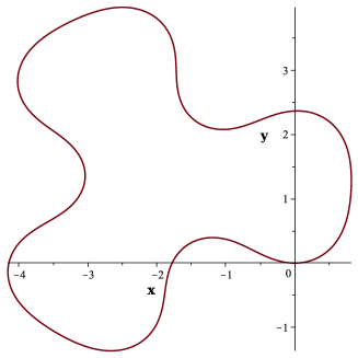
(a) A curve with Euclidean curvature (51).

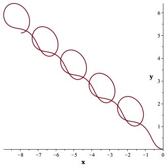
(b) A curve with Euclidean curvature (52).

Figure 5: Lemma 10 guarantees that the left curve is closed, but does not make any assertion about the right curve.

Theorem 12 (Euclidean estimate).

Let $\mathcal{C}_{1}$ and $\mathcal{C}_{2}$ be two $C^{2}$-smooth planar curves of the same Euclidean arc-length $L$. Assume $\kappa_{1}(s)$ and $\kappa_{2}(s)$, $s\in[0,L]$ are their respective Euclidean curvature functions. If $||\kappa_{1}-\kappa_{2}||_{[0,L]}\leq\delta$, then there exists $g\in SE(2)$, such that

$$d(\mathcal{C}_{1},g\,\mathcal{C}_{2})\leq\frac{\sqrt{2}}{2}{\delta L^{2}},$$ (53)

where $d$ is the Hausdorff distance.

Proof.

Identifying $\mathbb{R}^{2}$ with $\mathbb{C}$ and using Euler’s formula we may rewrite (48) as

$$\gamma(s)=\int_{0}^{s}e^{i\theta(t)}dt.$$ (54)

In what follows, we will use an important inequality, stating that a chord is shorter than the corresponding arc, illustrated in Figure 6:

$$\left|e^{i\theta_{1}}-e^{i\theta_{2}}\right|<|\theta_{1}-\theta_{2}|.$$ (55)

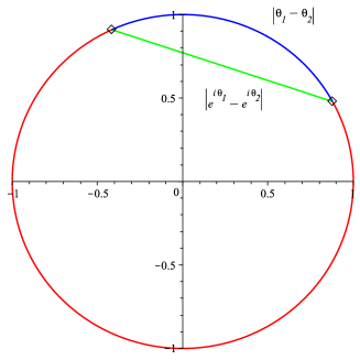
Figure 6: The length of the chord $|e^{i\theta_{1}}-e^{i\theta_{2}}|$ is shorter than the length of the arc $|\theta_{1}-\theta_{2}|$.

For $j=1,2$, let $\gamma_{j}(s)$, $s\in[0,L]$, be the Euclidean arc length parameterization of the curve $\mathcal{C}_{j}$. Then $T_{j}(s)=\gamma_{j}^{\prime}(s)$ and $N_{j}(s)=\gamma_{j}^{\prime\prime}(s)$ are the unit tangent and unit normal vectors, repectively, to $\mathcal{C}_{j}$. For $j=1,2$, there is a unique $g_{j}\in SE(2)$, such that

$$g_{j}\gamma_{j}(0)=(0,0),\quad g_{j}T_{j}(0)=(1,0),\quad g_{j}N_{j}(0)=(0,1).$$ (56)

It follows from Theorem 9, that for $j=1,2$, $\beta_{j}(t)=g_{j}\gamma_{j}(t)$ is given by equations (48) and so:

$$\left|g_{1}\gamma_{1}(s)-g_{2}\gamma_{2}(s)\right|=\left|\int_{0}^{s}e^{i\theta_{1}(t)}dt-\int_{0}^{s}e^{i\theta_{2}(t)}dt\right|\leq\int_{0}^{s}\left|e^{i\theta_{1}(t)}-e^{i\theta_{2}(t)}\right|dt$$ (57)

$$<\int_{0}^{s}\left|{\theta_{1}(t)}-{\theta_{2}(t)}\right|dt=\int_{0}^{s}\left|\int_{0}^{t}\left(\kappa_{1}(\tau)-\kappa_{2}(\tau)\right)d\tau\right|dt\leq\int_{0}^{s}\int_{0}^{t}\left|\kappa_{1}(\tau)-\kappa_{2}(\tau)\right|d\tau dt$$ (58)

$$\leq\int_{0}^{s}\int_{0}^{t}\left|\left|\kappa_{1}-\kappa_{2}\right|\right|_{[0,L]}d\tau dt\leq\int_{0}^{s}\int_{0}^{t}\delta d\tau dt=\frac{\delta s^{2}}{2}.$$ (59)

The inequality in line (57) follows from properties of definite integrals, the first inequality in line (58) follows from (55). The equality in line (58) follows from (49) and the properties of definite integrals. The first inequality in line (59) follows from (25).

Let $g=g_{1}^{-1}g_{2}$ then, using (31), (57)–(59) and the invariance of the Euclidean distance under the rigid motions, we have

$$d(\mathcal{C}_{1},g\,\mathcal{C}_{2})\leq\sqrt{2}\left|\left|\gamma_{1}-g\gamma_{2}\right|\right|_{[0,L]}=\sqrt{2}\sup_{s\in[0,L]}|\gamma_{1}(s)-g\gamma_{2}(s)|=\sqrt{2}\sup_{s\in[0,L]}|g_{1}\gamma_{1}(s)-g_{2}\gamma_{2}(s)|$$

$$\leq\sqrt{2}\frac{\delta L^{2}}{2}.$$

∎

If instead of the $L^{\infty}$-norm on the set of functions $\kappa$ we use the $L^{1}$-norm and require that $\int_{0}^{L}|\kappa_{1}(\tau)-\kappa_{2}(\tau)|d\tau\leq\delta$, then (58) implies the following result:

Theorem 13.

Let $\mathcal{C}_{1}$ and $\mathcal{C}_{2}$ be two $C^{2}$-smooth planar curves of the same Euclidean arc-length $L$. Assume $\kappa_{1}(s)$ and $\kappa_{2}(s)$, $s\in[0,L]$ are their respective Euclidean curvature functions and

$$\int_{0}^{L}|\kappa_{1}(\tau)-\kappa_{2}(\tau)|d\tau\leq\delta,$$ (60)

then there exists $g\in SE(2)$, such that

$$d(\mathcal{C}_{1},g\,\mathcal{C}_{2})\leq{\sqrt{2}}\delta L.$$

Proof.

The proof proceeds along the same lines as the proof of Theorem 12. However, the last inequality in (58) combined with (60) implies that

$$\left|g_{1}\gamma_{1}(s)-g_{2}\gamma_{2}(s)\right|<\int_{0}^{s}\delta dt=\delta s,$$

and so

$$d(\mathcal{C}_{1},g\,\mathcal{C}_{2})\leq\sqrt{2}\sup_{s\in[0,L]}|g_{1}\gamma_{1}(s)-g_{2}\gamma_{2}(s)|\leq{\sqrt{2}}\delta L.$$

∎

Example 14.

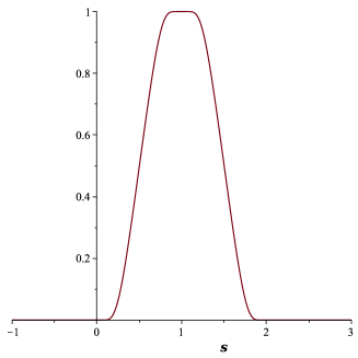
Figure 7: Bump function (61).

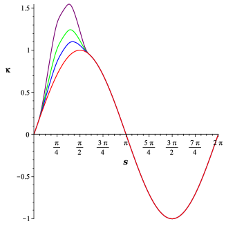
Figure 8: $\kappa^{*}_{10}(s)$, $\kappa^{*}_{20}(s)$, $\kappa^{*}_{40}(s)$, given by (62) and $\kappa(s)$$=\sin(s)$, $s\in[0,2\pi]$.

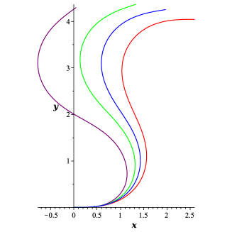
Figure 9: Curves $\mathcal{C}_{10}$, $\mathcal{C}_{20}$, $\mathcal{C}_{40}$, and $\mathcal{C}$, reconstructed from the Euclidean curvature functions in Figure 8.

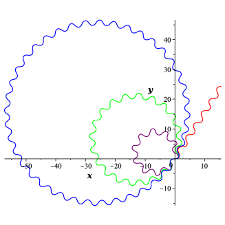
Figure 10: Closed curves reconstructed from periodic extensions $\kappa_{10}(s)$$,s\in[0,20\pi]$, $\kappa_{20}(s)$$,s\in[0,40\pi]$, $\kappa_{40}(s)$$,s\in[0,80\pi]$ of $\kappa^{*}_{n}$, shown in Figure 8, and an open curve reconstructed from $\kappa(s)$$=\sin(s)$, $s\in[0,12\pi]$.

To illustrate Theorems 12 and 13, we consider a curve whose Euclidean curvature function is $\kappa(s)=\sin(s)$ and a family of curves obtained by some variations of $\kappa(s)$. To define these variations consider a smooth bump function:

$$f(s)=\begin{cases}0&\text{if }s\leq 0,\\ \frac{e^{\frac{1}{1-s}}}{e^{\frac{1}{s}}+e^{\frac{1}{1-s}}}&\text{if }0<s<1,\\ 1&\text{if }s=1,\\ \frac{e^{\frac{1}{s-1}}}{e^{\frac{1}{s-1}}+e^{\frac{1}{2-s}}}&\text{if }1<s<2,\\ 0&\text{if }s\geq 2.\end{cases}$$ (61)

Next, for $n\in\mathbb{Z}\backslash\{0\}$, we define functions

$$\kappa_{n}^{*}(s)=\sin(s)+\frac{2\pi}{n}f(s)$$ (62)

on the closed interval $[0,2\pi]$ and let $\kappa_{n}(s)$ denote the periodic extension of $\kappa_{n}^{*}$ to $\mathbb{R}$. We observe that for any $L>0$,

$$||\kappa_{n}-\kappa||_{[0,L]}\leq\left|\left|\frac{2\pi}{n}f(s)\right|\right|_{[0,2]}\leq\frac{2\pi}{|n|}.$$

As $|n|\to\infty$, for $n>0$ and for $n<0$, the sequence $\kappa_{n}(s)$ uniformly converges to $\sin(s)$. In Figure 8, we show $\kappa_{10}(s)$, $\kappa_{20}(s)$, $\kappa_{40}(s)$, and $\kappa(s)=\sin(s)$ over their minimal period $[0,2\pi]$, while in Figure 10, we show curves $\mathcal{C}_{10}$, $\mathcal{C}_{20}$, $\mathcal{C}_{40}$, and $\mathcal{C}$ reconstructed from these curvatures with $s\in[0,2\pi]$. We observe that the Hausdorff distance between $\mathcal{C}$ and $\mathcal{C}_{n}$ decreases as $|n|$ increases (and so $\delta=\frac{2\pi}{|n|}$ decreases). At the same time, if we restrict $s$ to an interval $[0,L]$, with $0<L\leq 2\pi$, then for a fixed $n$, as $L$ increases, the distance between $\mathcal{C}$ and $\mathcal{C}_{n}$ increases.

Since $\int_{0}^{2}f(s)ds=1$, then $\int_{0}^{2\pi}\kappa_{n}(s)ds=\frac{2\pi}{n}$. Therefore, by Lemma 10, for $n\in\mathbb{Z}\setminus\{-1,0,1\}$, a curve reconstructed from $\kappa_{n}(s)$ with $s\in[0,2\pi n]$ is a closed curve with symmetry index $|n|$ and turning number 1. A curve reconstructed from $\kappa(s)=\sin(s)$ is, however, not closed. In Figure 10, we show the closed curves reconstructed from the curvatures $\kappa_{10}(s),s\in[0,20\pi]$, $\kappa_{20}(s),s\in[0,40\pi]$, $\kappa_{40}(s),s\in[0,80\pi]$, as well as an open curve reconstructed from $\kappa(s)=\sin(s)$, with $s\in[0,12\pi]$.

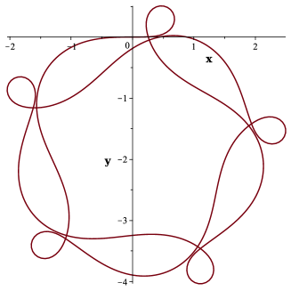
(a) A curve with curvature $\kappa_{5/3}(s)$, $s\in[0,10\pi]$ has turning number $3$ and $SE(2)$-symmetry index $5$.

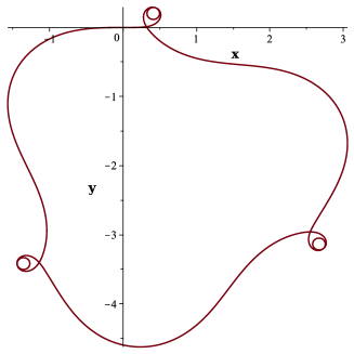
(b) A curve with curvature $\kappa_{3/5}$, $s\in[0,6\pi]$ has turning number $5$ and $SE(2)$-symmetry index $3$.

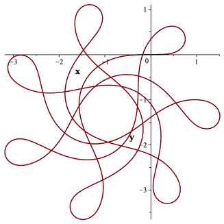
(c) A curve with curvature $\kappa_{7/3}$, $s\in[0,14\pi]$ has turning number $3$ and $SE(2)$-symmetry index $7$.

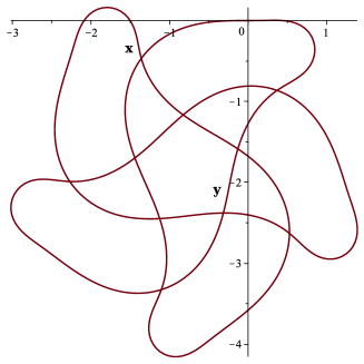
(d) A curve with curvature $\kappa_{-5/3}$, $s\in[0,10\pi]$ has turning number $-3$ and $SE(2)$-symmetry index $5$.

Figure 11: Closed curves reconstructed from $\kappa_{r}(s)$, where $r$ is a rational number.

It is worth noting that if, in formula (62), we replace the integer $n$ with a rational number $r=\frac{q}{\xi}$ such that $q\neq 1$ and $\xi$ are relatively prime then by Lemma 10, a curve reconstructed from $\kappa_{r}(s)$, $s\in[0,2\pi q]$ will be a closed curve with the $SE(2)$-symmetry index $q$ and turning number $\xi$. See Figure 11 for examples.

4 Affine reconstruction

In this section, we start by showing how Picard iterations can be used to reconstruct a curve from its affine curvature. We proceed by proving some upper bounds related to Picard iterations and using them to estimate how close, relative to the Hausdorff distance, two curves can be brought together by an special affine transformation, provided the affine curvature functions of the curves are $\delta$-close in the $L^{\infty}$-norm (Theorem 19).

Theorem 15 (Affine reconstruction).

Let $\mu(\alpha)$ be a continuous function on an interval $[0,L]$. Then there is a unique, up to an special affine transformation, curve $\mathcal{C}$ with the affine arc-length parametrization $\gamma(\alpha)=\left(x(\alpha),y(\alpha)\right)$, $\alpha\in[0,L]$, such that $\mu(\alpha)=x^{\prime\prime}(\alpha)y^{\prime\prime\prime}(\alpha)-y^{\prime\prime}(\alpha)x^{\prime\prime\prime}(\alpha)$ is its affine curvature function.

Proof.

According to (14), (19) and (20), $\gamma$ is a solution of the following system of first order differential equations:

$$\gamma^{\prime}(\alpha) =T(\alpha)$$ (63)

$$T^{\prime}(\alpha) =N(\alpha)$$ (64)

$$N^{\prime}(\alpha) =-\mu(\alpha)T(\alpha),$$ (65)

(equivalent to a third order ODE system of two decoupled equations $\gamma^{\prime\prime\prime}=-\mu\gamma^{\prime}$). Due to well known results on the existence and uniqueness of solutions to linear ODEs (see Theorems 5 and 6, Section 13.3 in [20]), there exists a unique solution of (63)-(65) with the initial data

$$\gamma(0)=(0,0),\quad T(0)=(1,0),\quad N(0)=(0,1).$$ (66)

Let $\gamma_{0}(\alpha)$ be such a solution parametrizing a curve $\mathcal{C}_{0}$. Let $\mathcal{C}_{1}$ be another curve with the affine arc-length parametrization $\gamma_{1}(\alpha)$, $\alpha\in[0,L]$, such that $\mu(\alpha)$ is its affine curvature. Let $T_{1}=\gamma_{1}^{\prime}(0)$ and $N_{1}=\gamma_{1}^{\prime\prime}(0)$. Then there exists a unique special affine transformation $g\in SA(2)$ which is a composition of a translation by the vector $-\gamma_{1}(0)$, followed by the unimodular linear transformation $\begin{pmatrix}T_{1}(0)\\ N_{1}(0)\end{pmatrix}^{-1}$, such that

$$g\cdot\gamma_{1}(0)=(0,0),\quad g\cdot T_{1}=(1,0),\quad g\cdot N_{1}=(0,1).$$

Since $\mu$ and $d\alpha$ are special affine invariant, it follows that the curve $g\,\mathcal{C}_{1}$ parametrized by $g\gamma_{1}$ satisfies(63)-(65) with the same initial data (66) and, therefore, $\mathcal{C}_{0}=g\,\mathcal{C}_{1}$. ∎

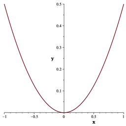
(a) $\mu=0$.

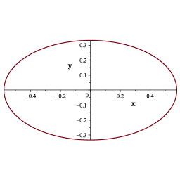
(b) $\mu=2$.

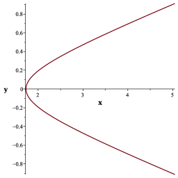
(c) $\mu=-3$.

Figure 12: Examples of curves with constant special affine curvature functions.

We now consider computational aspects of reconstruction of a curve from its affine curvature. Once $T(\alpha)$ is known, $\gamma$ can be reconstructed by integration which can be done exactly or numerically depending on the complexity of $T(\alpha)$. To find $T(\alpha)$, one needs to solve the system (64)-(65).

When $\mu(\alpha)$ is a constant function, standard methods can be applied. In fact, as shown in [12], if $\mu=0$ then the reconstructed curve, with the initial conditions (66), is a parabola $\gamma=(\alpha,\frac{1}{2}\alpha^{2})$. When $\mu>0$ then $\gamma=\left(\frac{\sin(\sqrt{\mu}\alpha)}{\sqrt{\mu}},-\frac{\cos(\sqrt{\mu}\alpha)}{\mu}\right)$, an ellipse. When $\mu<0$ then $\gamma=\left(\sqrt{|\mu|}\cosh(\sqrt{|\mu|}\alpha),\frac{\sinh(\sqrt{|\mu|}\alpha)}{|\mu|}\right)$, a hyperbola. See Figure 12 for specific examples.

When $\mu$ is non-constant but analytic one can use power series methods to find the solutions. The power series solutions for the case when $\mu$ is a monomial: $\mu=c\alpha^{k}$ are given in the Appendix. For an arbitrary continuous function $\mu$, we approximate $T(\alpha)$ by applying Picard iterations as follows.

As discussed in Section 2.3, equations (64) and (65) are equivalent to the matrix equation (23), where $A(\alpha)=\begin{pmatrix}{}T(\alpha)\\ N(\alpha)\\ \end{pmatrix}$ is the affine frame matrix and $C(\alpha)$ is the affine Cartan matrix given by (24). The Picard iterations are defined as follows:

$$A_{0}(\alpha) =A_{0}$$

$$A_{n}(\alpha) =A_{0}+\int_{0}^{\alpha}C(t)A_{n-1}(t)dt,\text{ for }n>0.$$ (67)

It is well known that on any interval $[0,L]$, as $n\to\infty$ the sequence of $\left\{A_{n}(\alpha)\right\}$ uniformly converges to the unique matrix of continuous functions $A(\alpha)$, satisfying the integral equation

$$A(\alpha)=A_{0}+\int_{0}^{\alpha}C(t)A(t)dt$$ (68)

and, therefore, the differential equation (23) with the initial value $A_{0}$. A direct proof for the convergence of (67) to the solutions of (23) with the initial value $A_{0}$, where $C$ is an arbitrary continuous matrix, is given in [12] Lemma 2-12.

Example 16.

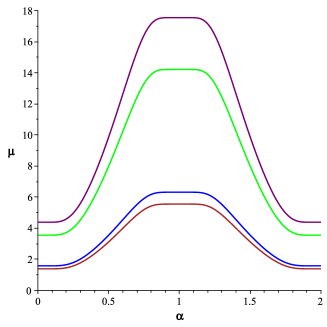
Figure 13: $\mu^{*}_{2/3}(\alpha)$, $\mu^{*}_{3/5}(\alpha)$, $\mu^{*}_{2/5}(\alpha)$, and $\mu^{*}_{3/8}(\alpha)$, $\alpha\in[0,2]$ given by (69).

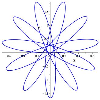
(a) Approximation of a curve with equi-affine curvature $\mu_{2/5}$ on $[0,22]$.

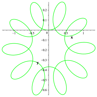
(b) Approximation of a curve with equi-affine curvature $\mu_{3/5}$ on $[0,20]$.

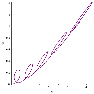
(c) Approximation of a curve with equi-affine curvature $\mu_{2/3}$ on $[0,10]$.

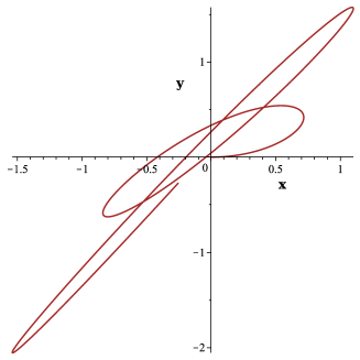
(d) Approximation of a curve with equi-affine curvature $\mu_{3/8}$ on $[0,8]$.

Figure 14: Approximations of curves, using 200 Picard iterations, reconstructed from periodic extensions of the affine curvature functions shown in Figure 13.

We will briefly look at a few curves that are reconstructed from their affine curvatures. Recall the bump function $f(s)$ given by (61). Let

$$\mu_{n}^{*}(\alpha)=n^{2}\pi^{2}(f(\alpha)+1)^{2}$$ (69)

with domain $[0,2]$ and let $\mu_{n}(\alpha)$ be the periodic extension of $\mu_{n}^{*}$ to $\mathbb{R}$. In Figure 14, we show approximations (using 200 Picard iterations) of curves with affine curvatures $\mu_{2/3}$, $\mu_{2/5}$, $\mu_{3/5}$, and $\mu_{3/8}$, initial conditions $\gamma(0)=(0,0)$, and $A_{0}=I$.

It is important to note that the affine analog to Lemma 10 is not valid. Indeed, it is shown, for instance, in Example 7.2 in [18], that in contrast with the Euclidean case, the total special affine curvature $\int\mu d\alpha$ of a closed curve is not topologically invariant, and thus it can not be used to determine whether the curve is closed or open. Moreover, as remarked in [23] on p. 421, there does not exist a function of $\mu$ whose integral is a topological invariant. With this in mind, it is worth noting that the approximations of the curves with special affine curvatures $\mu_{2/5}$ and $\mu_{3/5}$ appear to be closed, while the curves with the affine curvature functions $\mu_{2/3}$ and $\mu_{3/8}$ show no sign that they would close if their domain was extended.

We now investigate the “closeness” of two curves reconstructed from “close” affine curvatures. We start by establishing certain upper bounds:

Lemma 17.

Assume that $||C||_{[0,L]}=\max\{1,||\mu||_{[0,L]}\}=c$. Let $A_{n}$ be defined by the Picard iterations (67) and $A$ be the limit of these iterations. Then for any $\alpha\in[0,L]$ the following inequalities hold:

$$\left<A_{n}\right>(\alpha) \leq\left<A_{0}\right>\sum_{i=0}^{n}\frac{(c\alpha)^{i}}{i!},$$ (70)

$$\left<A\right>(\alpha) \leq\left<A_{0}\right>e^{c\alpha},$$ (71)

$$\left<A_{n}-A_{n-1}\right>(\alpha) \leq\left<A_{0}\right>\frac{(c\alpha)^{n}}{n!},$$ (72)

$$\left<A_{n}-A\right>(\alpha) \leq\left<A_{0}\right>e^{c\alpha}\frac{(c\alpha)^{n+1}}{(n+1)!}.$$ (73)

Proof.

1. For $n=0$, (70) states that $\left<A_{0}\right>\leq\left<A_{0}\right>$, which is trivially true. We proceed by induction. Assume that (70) holds for all $0\leq k<n$. Then from (67), (29) and the triangle inequality, we have

   $$\left<A_{n}\right>(\alpha)\leq\left<A_{0}\right>+\int_{0}^{\alpha}\left<CA_{n-1}\right>(t)dt.$$ (74)

   Note that for any matrix $A=\begin{pmatrix}a_{11}&a_{12}\\ a_{21}&a_{22}\end{pmatrix}$, we have $CA=\begin{pmatrix}a_{21}&a_{22}\\ -\mu a_{11}&-\mu a_{12}\end{pmatrix}$ and, therefore, since $c\geq||\mu||_{[0,L]}$ and $c\geq 1$,

   $$\left<CA\right>(t)\leq c\left<A\right>(t).$$ (75)

   Returning to (74) and using the inductive assumption, we then have

   $$\left<A_{n}\right>(\alpha)\leq\left<A_{0}\right>+c\int_{0}^{\alpha}\left<A_{n-1}\right>(t)dt\leq\left<A_{0}\right>+c\left<A_{0}\right>\sum_{i=0}^{n-1}\int_{0}^{\alpha}\frac{(ct)^{i}}{i!}\,dt$$ (76)

   $$=\left<A_{0}\right>\left(1+c\,\sum_{i=0}^{n-1}\frac{c^{i}\alpha^{i+1}}{(i+1)!}\right)=\left<A_{0}\right>\left(1+\sum_{i=1}^{n}\frac{c^{i}\alpha^{i}}{i!}\right)=\left<A_{0}\right>\sum_{i=0}^{n}\frac{(c\alpha)^{i}}{i!}.$$

2. To show (71), we use (39) and (70)

   $$\left<A\right>(\alpha)=\lim_{n\to\infty}\left<A_{n}\right>(\alpha)\leq\left<A_{0}\right>\sum_{i=0}^{\infty}\frac{(c\alpha)^{i}}{i!}=\left<A_{0}\right>e^{c\alpha}.$$ (77)

3. For $n=1$, (72) states that $\left<A_{1}-A_{0}\right>(\alpha)\leq\left<A_{0}\right>c\alpha$. This, indeed, holds because by (67) $A_{1}(\alpha)-A_{0}(\alpha)=\int_{0}^{\alpha}C(t)A_{0}dt$, and so by (29) and (75)

   $$\left<A_{1}-A_{0}\right>(\alpha)\leq\int_{0}^{\alpha}\left<C(t)A_{0}\right>dt\leq\int_{0}^{\alpha}c\left<A_{0}\right>dt=\left<A_{0}\right>c\alpha.$$

   We proceed by induction. Assume that (72) holds for all $1\leq k<n$. By (67),

   $$A_{n}(\alpha)-A_{n-1}(\alpha)=\int_{0}^{\alpha}C(t)(A_{n-1}(t)-A_{n-2}(t))dt,$$

   and then by (29), (75), and the inductive hypothesis

   $$\left<A_{n}-A_{n-1}\right>(\alpha)\leq\int_{0}^{\alpha}c\left<A_{n-1}-A_{n-2}\right>(t)dt\leq\left<A_{0}\right>\int_{0}^{\alpha}c\frac{(ct)^{n-1}}{(n-1)!}dt=\left<A_{0}\right>\frac{(c\alpha)^{n}}{n!}.$$

4. To show (73), we note that for any integer $j>0$, due to the triangle inequality and (72), we have

   $$\left<A_{n}-A\right>(\alpha) \leq\left<A_{n}-A_{n+1}\right>(\alpha)+\left<A_{n+1}-A_{n+2}\right>(\alpha)+\dots$$ (78)

   $$+\left<A_{n+j-1}-A_{n+j}\right>(\alpha)+\left<A_{n+j}-A\right>(\alpha)\leq\left<A_{0}\right>\sum_{i={n+1}}^{n+j}\frac{(c\alpha)^{i}}{i!}+\left<A_{n+j}-A\right>(\alpha).$$

   Since $A_{n+j}(\alpha)$ converges to $A(\alpha)$ as $j\to\infty$, $\lim_{j\to\infty}\left<A_{n+j}-A\right>(\alpha)=0$, and so (78) implies

   $$\left<A_{n}-A\right>(\alpha)\leq\left<A_{0}\right>\sum_{i={n+1}}^{\infty}\frac{(c\alpha)^{i}}{i!}=\left<A_{0}\right>\left(e^{c\alpha}-\sum_{i={0}}^{n}\frac{(c\alpha)^{i}}{i!}\right).$$ (79)

   Due to Taylor’s remainder theorem, there exists $\alpha_{0}\in[0,\alpha]$, such that

   $$R_{n}=e^{c\alpha}-\sum_{i={0}}^{n}\frac{(c\alpha)^{i}}{i!}=e^{c\alpha_{0}}\frac{(c\alpha)^{n+1}}{(n+1)!}\leq e^{c\alpha}\frac{(c\alpha)^{n+1}}{(n+1)!},$$

   where the last inequality is true because $c>0$ and so $e^{c\alpha}$ is an increasing function.

∎

Next, we establish the bounds on the distance between two affine frames reconstructed from two $\delta$-close (in the $L^{\infty}$ norm) affine curvature functions. This result is consistent with a well known ODE result of continuous dependence of the solutions of an ODE on its parameters (see, for instance, Theorem 10, Section 13.4 in [20] and Theorem 3, Chapter 5 in [2]).

Proposition 18.

Let $\mu(\alpha)$ and $\tilde{\mu}(\alpha)$ be two continuous functions on the interval $[0,L]$ and let $C$ and $\tilde{C}$ be corresponding Cartan’s matrices defined by (24). Let $\hat{c}=\max\{1,||\mu||_{[0,L]},||\tilde{\mu}||_{[0,L]}\}$. Let $A_{n}$ and $\tilde{A}_{n}$ be defined by the Picard iterations (67) for the given matrices $C$ and $\tilde{C}$, respectively, and $A$, $\tilde{A}$ be the limits of these iterations. If $||\mu-\tilde{\mu}||_{[0,L]}\leq\delta$, then for all $\alpha\in[0,L]$:

$$\left<A_{n}-\tilde{A}_{n}\right>(\alpha) \leq\left<A_{0}\right>\delta\alpha\sum_{i=0}^{n-1}\frac{(\hat{c}\alpha)^{i}}{i!}\qquad\text{ for }n>0$$ (80)

and

$$\left<A-\tilde{A}\right>(\alpha) \leq\left<A_{0}\right>\delta\alpha e^{\hat{c}\alpha}.$$ (81)

Proof.

1. We first observe that for all $\alpha\in[0,L]$, $\left<C-\tilde{C}\right>(\alpha)=|\mu(\alpha)-\tilde{\mu}(\alpha)|<\delta$.

   For $n=1$, (80) states that $\left<A_{1}-\tilde{A}_{1}\right>(\alpha)\leq\left<A_{0}\right>\delta\alpha$. This, indeed, holds because by (67), keeping in mind that $A_{0}(\alpha)=\tilde{A}_{0}(\alpha)=\left<A_{0}\right>$, we have

   $$\left<A_{1}-\tilde{A}_{1}\right>(\alpha) \leq\int_{0}^{\alpha}\left<(C-\tilde{C})A_{0}\right>(t)dt\leq\int_{0}^{\alpha}\left<A_{0}\right>|\tilde{\mu}(t)-\mu(t)|dt$$

   $$\leq\left<A_{0}\right>\int_{0}^{\alpha}\delta dt=\left<A_{0}\right>\delta\alpha.$$

   We proceed by induction. Assume that (80) holds for all $1\leq k<n$, then

   $$\left<A_{n}-\tilde{A}_{n}\right>(\alpha)\leq\int_{0}^{\alpha}\left<CA_{n-1}-\tilde{C}\tilde{A}_{n-1}\right>(t)dt$$ (82)

   $$=\int_{0}^{\alpha}\left<CA_{n-1}-C\tilde{A}_{n-1}+C\tilde{A}_{n-1}-\tilde{C}\tilde{A}_{n-1}\right>(t)dt$$

   $$\leq\int_{0}^{\alpha}\hat{c}\left<A_{n-1}-\tilde{A}_{n-1}\right>(t)dt+\int_{0}^{\alpha}\delta\left<\tilde{A}_{n-1}\right>(t)dt$$ (83)

   $$\leq\int_{0}^{\alpha}\hat{c}\left<A_{0}\right>\delta t\sum_{i=0}^{n-2}\frac{(\hat{c}t)^{i}}{i!}dt+\int_{0}^{\alpha}\left<A_{0}\right>\delta\sum_{i=0}^{n-1}\frac{(\hat{c}t)^{i}}{i!}dt$$ (84)

   $$=\left<A_{0}\right>\delta\left(\hat{c}\sum_{i=0}^{n-2}\frac{\hat{c}^{i}\alpha^{i+2}}{i!(i+2)}+\sum_{i=0}^{n-1}\frac{\hat{c}^{i}\alpha^{i+1}}{(i+1)!}\right)$$

   $$=\left<A_{0}\right>\delta\left(\sum_{i=1}^{n-1}\frac{\hat{c}^{i}\alpha^{i+1}}{(i-1)!(i+1)}+\sum_{i=0}^{n-1}\frac{\hat{c}^{i}\alpha^{i+1}}{(i+1)!}\right)$$

   $$=\left<A_{0}\right>\delta\left(\alpha+\sum_{i=1}^{n-1}\hat{c}^{i}\alpha^{i+1}\left(\frac{1}{(i-1)!(i+1)}+\frac{1}{(i+1)!}\right)\right)$$

   $$=\left<A_{0}\right>\delta\alpha\left(1+\sum_{i=1}^{n-1}\hat{c}^{i}\alpha^{i}\frac{1}{i!}\right)=\left<A_{0}\right>\delta\alpha\sum_{i=0}^{n-1}\frac{(\hat{c}\alpha)^{i}}{i!},$$

   where, in line (82), we use (67), (29), and the triangle inequality. In line (83), we use (75) and the triangle inequality, and in line (84), we use the inductive assumption and (70).

2. To show (81), we note that since $A_{n}(\alpha)$ and $\tilde{A}_{n}(\alpha)$ converge to $A(\alpha)$ and $\tilde{A}(\alpha)$, respectively, as $n\to\infty$, then by (39), $\lim_{n\to\infty}\left<A_{n}-\tilde{A}_{n}\right>(\alpha)=\left<A-\tilde{A}\right>(\alpha)$, and so taking the limit of both sides in the inequality (80) as $n\to\infty$, we obtain (81).

∎

In the next theorem, we establish an upper bound on how close (in the Hausdorff distance) two curves with $\delta$-close (in the $L^{\infty}$-norm) affine curvature functions can be brought together by a special affine transformation.

Theorem 19 (Affine estimate).

Let $\mathcal{C}_{1}$ and $\mathcal{C}_{2}$ be two $C^{3}$-smooth planar curves of the same affine arc-length $L$. Assume $\mu_{1}(\alpha)$ and $\mu_{2}(\alpha)$, $\alpha\in[0,L]$ are their respective affine curvature functions. Assume further that $\mathcal{C}_{2}$ satisfies the initial conditions (66). If $||\mu_{1}-\mu_{2}||_{[0,L]}\leq\delta$ and $\hat{c}=\max\{1,\left|\left|\mu_{1}\right|\right|_{[0,L]},\left|\left|\mu_{2}\right|\right|_{[0,L]}\}$, then there is $g\in SA(2)$, such that

$$d(g\,\mathcal{C}_{1},\mathcal{C}_{2})\leq\sqrt{2}\frac{\delta L}{\hat{c}}(e^{\hat{c}L}-1),$$ (85)

where $d$ is the Hausdorff distance.

Proof.

For $i=1,2$, let $\gamma_{i}(\alpha)$, $\alpha\in[0,L]$ be the affine-arc length parameterization of $\mathcal{C}_{i}$, while $T_{i}(\alpha)=\gamma_{i}^{\prime}(\alpha)$ and $N_{i}(\alpha)=\gamma_{i}^{\prime\prime}(\alpha)$ are the affine frame vectors along the corresponding curves. Then, there is a unique $g\in SA(2)$, such that

$$g\gamma_{1}(0)=\gamma_{2}(0)=(0,0),\quad gT_{1}(0)=T_{2}(0)=(1,0),\quad gN_{1}(0)=N_{2}(0)=(0,1).$$ (86)

Due to the $SA(2)$-invariance of the affine curvature function, the curve $g\,\mathcal{C}_{1}$ parametrized by $g\gamma_{1}(\alpha)$ has affine curvature function $\mu_{1}(\alpha)$. It follows from Theorem 15, that $g\gamma_{1}(\alpha)$ is the unique solution of (63)-(65), with $\mu(\alpha)=\mu_{1}(\alpha)$ and $\gamma_{2}(\alpha)$ is the unique solution of (63)-(65), with $\mu(\alpha)=\mu_{2}(\alpha)$, both with initial conditions (86).

Denote the affine frame of $g\,\mathcal{C}_{1}$ as $A(\alpha)=\begin{pmatrix}gT_{1}(\alpha)\\ gN_{1}(\alpha)\end{pmatrix}$ and the affine frame of $\mathcal{C}_{2}$ as $\tilde{A}(\alpha)=\begin{pmatrix}T_{2}(\alpha)\\ N_{2}(\alpha)\end{pmatrix}$. Then

$$\left<gT_{1}-T_{2}\right>(\alpha)\leq\left<A-\tilde{A}\right>(\alpha)\leq\delta\alpha e^{\hat{c}\alpha},$$ (87)

where the first inequality is due to the definition of $\left<\cdot\right>$ and the second inequality is due to (81). Since $g\gamma_{1}(\alpha)=\int_{0}^{\alpha}T_{1}(t)dt+T_{0}$ and $\gamma_{2}(\alpha)=\int_{0}^{\alpha}T_{2}(t)dt+T_{0}$, we have for all $\alpha\in[0,L]$:

$$|g\gamma_{1}(\alpha)-\gamma_{2}(\alpha)|\leq\int_{0}^{\alpha}\left<gT_{1}-T_{2}\right>(t)dt\leq\int_{0}^{\alpha}\delta te^{\hat{c}t}dt\leq\int_{0}^{\alpha}\delta Le^{\hat{c}t}dt=\frac{\delta L}{\hat{c}}(e^{\hat{c}\alpha}-1).$$ (88)

It then follows from (31) and (88) that

$$d(g\,\mathcal{C}_{1},\mathcal{C}_{2})\leq\sqrt{2}\left|\left|g\gamma_{1}-\gamma_{2}\right|\right|_{[0,L]}\leq\sqrt{2}\sup_{\alpha\in[0,L]}|g\gamma_{1}(\alpha)-\gamma_{2}(\alpha)|\leq\sqrt{2}\frac{\delta L}{\hat{c}}(e^{\hat{c}L}-1).$$

∎

5 Conclusion

In this paper, we considered practical aspects of reconstructing planar curves with prescribed Euclidean or affine curvatures. An immediate extension of the current work would be the reconstruction of planar curves with prescribed projective curvatures, and obtaining distance estimates between curves, modulo a projective transformation, compared to the distance between the projective curvatures. Indeed, the projective group, containing both the special Euclidean and the special affine groups, plays a crucial role in computer vision (see, for, instance [5] and [13]). Extension to space curves is another direction with immediate applications.

By considering specific group actions, we take advantage of their specific structural properties and obtain results that can be immediately suitable for applications. However, the generalization of the moving frame method by Fels and Olver, [6, 16], allows us, in principle, to generalize our approach to an action of an arbitrary Lie group $G$ on curves (or even on higher dimensional submanifolds) in some ambient metric space. In such generalization, a $G$-equivariant moving frame map from the corresponding jet space to the group $G$ plays the role of $G$-frame matrix $A$, appearing in this paper, and we will seek an estimate of how close two submanifolds can be brought together by an element of $G$, provided the Maurer-Cartan invariants for the $G$-action are sufficiently close.

In this paper, we used the Hausdorff distance between curves when considering both the $SE(2)$- and the $SA(2)$-actions on the plane. However, while the Hausdorff distance is $SE(2)$-invariant, it is not $SA(2)$-invariant and so it does not provide a natural measure of distance between two curves in the special affine case. In a future work, it is worthwhile to explore $SA(2)$-invariant alternatives for measuring distance between two curves, based, for instance, on the area of the region between two curves. In the generalization to other group actions, the goal would be to consider a $G$ -invariant distance between two submanifolds.

6 Appendix

If a given special affine curvature is analytic, it is possible to reconstruct the corresponding curve by looking for power series solutions to the second order ODE system $T_{\alpha\alpha}=-\mu(\alpha)T$. We illustrate this approach by reconstructing curves whose special affine curvatures are of the form $\mu(\alpha)=c\alpha^{k}$ for $c\in\mathbb{R}$ and $k\in\mathbb{N}$.

Proposition 20.

For $c\in\mathbb{R}$, $k\in\mathbb{N}$ and $T_{0},N_{0}\in\mathbb{R}^{2}$, such that $\det[T_{0},N_{0}]=1$, the affine tangent vector along a curve, whose affine curvature function is $\mu(\alpha)=c\alpha^{k}$ for $c\in\mathbb{R}$ and $k\in\mathbb{N}$, the initial affine tangent vector is $T_{0}$ and the initial affine normal is $N_{0}$, is given by the absolutely convergent power series

$$T(\alpha)=-T_{0}\Gamma\left(-\frac{1}{K}\right)\sum\limits_{i=1}^{\infty}\frac{(-c)^{i}\alpha^{Ki}}{i!K^{2i+1}\Gamma\left(-\frac{1}{K}+i+1\right)}+N_{0}\Gamma\left(\frac{1}{K}\right)\sum\limits_{i=1}^{\infty}\frac{(-c)^{i}\alpha^{K(i+1)}}{i!K^{2i+1}\Gamma\left(\frac{1}{K}+i+1\right)},$$ (89)

where $K=k+2$ and $\Gamma$ denotes the gamma function.

Proof.

We first represent the tangent vector $T(\alpha)$ by

$$T=b_{0}+b_{1}\alpha+b_{2}\alpha^{2}+b_{3}\alpha^{3}+\cdots+b_{n}\alpha^{n}\cdots$$ (90)

where each $b_{i}$ is a vector coefficient, with $b_{0}=T_{0}$ and $b_{1}=N_{0}$ being the initial values of the affine tangent and the affine normal, respectively.

We write out the power series representation of $T_{\alpha\alpha}$ and $-c\alpha^{k}T$:

$$T_{\alpha\alpha}=0b_{0}+0b_{1}\alpha+2b_{2}+3\cdot 2b_{3}\alpha+\cdots+n(n-1)b_{n}\alpha^{n-2}\cdots$$ (91)

$$-c\alpha^{k}T=-cb_{0}\alpha^{k}-cb_{1}\alpha^{(k+1)}-cb_{2}\alpha^{(k+2)}-cb_{3}\alpha^{(k+3)}-\cdots-cb_{n}\alpha^{(k+n)}-\cdots$$ (92)

The equality of these two power series implies the equality of vector-coefficients with the same powers of $\alpha$ in two series. It follows that

$$b_{n}=\begin{cases}0&\text{ when }2\leq n\leq k+1\\ -\dfrac{cb_{n-(k+2)}}{n(n-1)}&\text{ when }n\geq k+2\end{cases}.$$ (93)

Then $b_{k+2}$ and $b_{k+3}$ can be written in terms of $b_{0}$ and $b_{1}$:

$$b_{k+2}=-\frac{cb_{0}}{(k+2)(k+1)},\qquad b_{k+3}=-\frac{cb_{1}}{(k+3)(k+2)}.$$ (94)

Using induction, when $n\mod(k+2)=0$, we can express $b_{n}$ in terms of $b_{0}$, when $n\mod(k+2)=1$, we can express $b_{n}$ in terms of $b_{1}$, and we can show that otherwise $b_{n}=0$. This gives us the power series representation for $T$ in terms of $b_{0}$ and $b_{1}$ as

$$T(\alpha)=b_{0}+b_{1}\alpha+\sum\limits_{i=1}^{\infty}(-c\alpha^{k+2})^{i}\Bigg{(} \left(\prod_{j=1}^{i}\frac{1}{j(k+2)\left(j\left(k+2\right)-1\right)}\right)b_{0}+$$

$$\left(\prod_{j=1}^{i}\frac{1}{j\left(k+2\right)\left(j\left(k+2\right)+1\right)}\right)b_{1}\alpha\Bigg{)}.$$ (95)

We can split (95) into two parts:

$$B_{0}= b_{0}\sum\limits_{i=1}^{\infty}\left(\prod_{j=1}^{i}\frac{1}{j(k+2)(j(k+2)-1)}\right)(-c\alpha^{k+2})^{i}$$ (96)

$$={b_{0}\sum\limits_{i=1}^{\infty}\left(\prod_{j=1}^{i}\frac{1}{(j(k+2)-1)}\right)\frac{(-c\alpha^{k+2})^{i}}{i!(k+2)^{i}}=b_{0}\sum\limits_{i=1}^{\infty}\Psi_{-}(K,i)\frac{(-c\alpha^{K})^{i}}{i!K^{i}}}$$

and

$$B_{1}= b_{1}\sum\limits_{i=1}^{\infty}\left(\prod_{j=1}^{i}\frac{1}{j(k+2)(j(k+2)+1)}\right)(-c\alpha^{k+2})^{i}\alpha$$ (97)

$$=b_{1}\sum\limits_{i=1}^{\infty}\left(\prod_{j=1}^{i}\frac{1}{(j(k+2)+1)}\right)\frac{(-c\alpha^{k+2})^{i}\alpha}{i!(k+2)^{i}}=b_{1}\sum\limits_{i=1}^{\infty}\Psi_{+}(K,i)\frac{(-c\alpha^{K})^{i}\alpha}{i!K^{i}},$$

where $K=k+2$ and

$$\Psi_{-}(K,i) =\prod_{j=1}^{i}\frac{1}{(jK-1)}=\frac{1}{K^{i}}\frac{1}{\prod_{j=1}^{i}(j-\frac{1}{K})}$$ (98)

$$\Psi_{+}(K,i) =\prod_{j=1}^{i}\frac{1}{(jK+1)}=\frac{1}{K^{i}}\frac{1}{\prod_{j=1}^{i}(j+\frac{1}{K})}.$$ (99)

These functions involve what is called rising factorials, defined by

$$z^{\bar{i}}:=z(z+1)\cdots(z+i-1)=\prod_{j=0}^{i-1}(z+j).$$

Rising factorials can be expressed in terms of $\Gamma$ functions, $\Gamma(z)=\int_{0}^{\infty}x^{z-1}e^{-x}dx$, as

$$z^{\bar{i}}=\frac{\Gamma(z+i)}{\Gamma(z)}.$$

For details see formulas (5.84), (5.85) and (5.89) on pp. 210-211 of [11]. Since

$$\prod_{j=1}^{i}\left(j-\frac{1}{K}\right)=-K\left(-\frac{1}{K}\right)^{\overline{i+1}}=-K\frac{\Gamma\left(-\frac{1}{K}+i+1\right)}{\Gamma\left(-\frac{1}{K}\right)},$$ (100)

$$\prod_{j=1}^{i}\left(j+\frac{1}{K}\right)=K\left(\frac{1}{K}\right)^{\overline{i+1}}=K\frac{\Gamma\left(\frac{1}{K}+i+1\right)}{\Gamma\left(\frac{1}{K}\right)},$$ (101)

we can rewrite (98)-(99) using $\Gamma$ functions:

$$\Psi_{-}(K,i) =\prod_{j=1}^{i}\frac{1}{(jK-1)}=-\frac{1}{K^{i+1}}\frac{\Gamma\left(-\frac{1}{K}\right)}{\Gamma\left(-\frac{1}{K}+i+1\right)},$$ (102)

$$\Psi_{+}(K,i) =\prod_{j=1}^{i}\frac{1}{(jK+1)}=\frac{1}{K^{i+1}}\frac{\Gamma\left(\frac{1}{K}\right)}{\Gamma\left(\frac{1}{K}+i+1\right)}.$$ (103)

Therefore,

$$B_{0}(\alpha)= b_{0}\sum\limits_{i=1}^{\infty}\Psi_{-}(K,i)\frac{(-c\alpha^{K})^{i}}{i!K^{i}}$$

$$=b_{0}\sum\limits_{i=1}^{\infty}\left(-\frac{1}{K^{i+1}}\frac{\Gamma\left(-\frac{1}{K}\right)}{\Gamma\left(-\frac{1}{K}+i+1\right)}\right)\frac{(-c\alpha^{K})^{i}}{i!K^{i}}$$

$$=-b_{0}\Gamma\left(-\frac{1}{K}\right)\sum\limits_{i=1}^{\infty}\frac{1}{\Gamma\left(-\frac{1}{K}+i+1\right)}\frac{(-c\alpha^{K})^{i}}{i!K^{2i+1}},$$ (104)

$$B_{1}(\alpha)= b_{1}\sum\limits_{i=1}^{\infty}\Psi_{+}(K,i)\frac{(-c\alpha^{K})^{i}\alpha}{i!K^{i}}$$

$$=b_{1}\sum\limits_{i=1}^{\infty}\left(\frac{1}{K^{i+1}}\frac{\Gamma\left(\frac{1}{K}\right)}{\Gamma\left(\frac{1}{K}+i+1\right)}\right)\frac{(-c\alpha^{K})^{i}\alpha}{i!K^{i}}$$

$$=b_{1}\Gamma\left(\frac{1}{K}\right)\sum\limits_{i=1}^{\infty}\frac{1}{\Gamma\left(\frac{1}{K}+i+1\right)}\frac{(-c\alpha^{K})^{i}\alpha}{i!K^{2i+1}}.$$ (105)

Convergence of series (95) for all $\alpha$ follows from a general known result (Theorem 39.22 p.560 [22]). Directly, absolute convergence of sub-series (96) and (97) can be verified by the ratio test, implying absolute convergence of series (95). ∎

The power series for the affine arc-length parameterization $\gamma(\alpha)$ is obtained by integrating the series $T(\alpha)$. See Figures 16 and 16 for reconstructions of curves with curvatures $\mu(\alpha)=\alpha$ and $\mu(\alpha)=\alpha^{2}$ respectively.

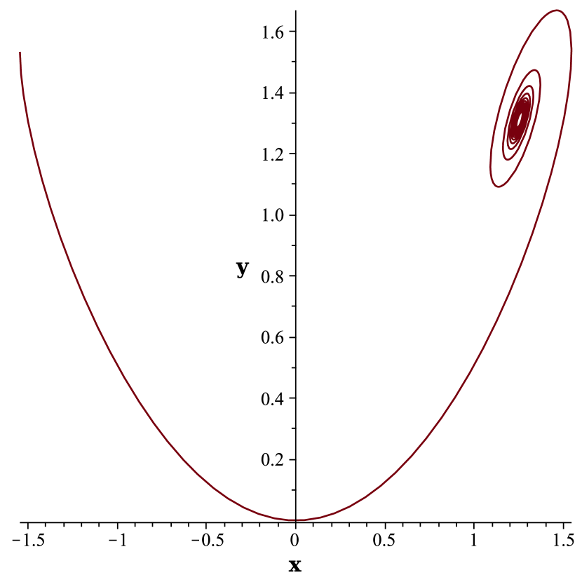
Figure 15: Curve with special affine curvature $\mu(\alpha)=\alpha$

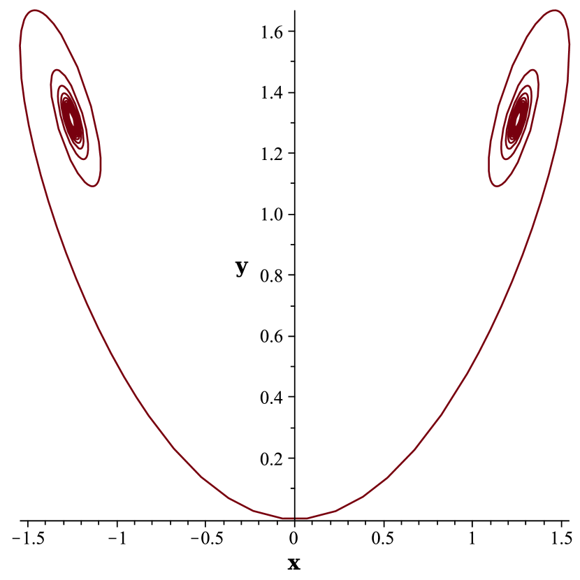
Figure 16: Curve with special affine curvature $\mu(\alpha)=\alpha^{2}$

Remark 21.

The system $T_{\alpha\alpha}=-c\alpha^{k}T$ consists of two decoupled equations of the type $u^{\prime\prime}(\alpha)=-c\alpha^{k}u(\alpha)$, whose general solution in terms of of the Bessel functions, can be found, for instance, in Section 14.1.2, subsection 7, number 3 of [21]. The Bessel functions can be expended into power series involving the gamma function, recovering series (89). The advantage of formula (89) is in its explicit dependence on the initial vectors $T_{0}$ and $N_{0}$. In addition, our direct proof illustrates how the power series approach can be applied for other analytic affine curvatures $\mu(\alpha)$.

Acknowledgement:

This work was performed during the REU 2020 program at the North Carolina State University (NCSU) and was supported by the Department of Mathematics at NCSU and the NSA grant H98230-20-1-0259. At the time when the project was performed, Jose Agudelo was an undergraduate student at North Dakota State University, Brooke Dippold was an undergraduate student at Longwood University, Ian Klein was an undergraduate student at Carleton College, Alex Kokot was an undergraduate student at the University of Notre Dame, Eric Geiger was a graduate student at NCSU. Irina Kogan is a Professor of Mathematics at NCSU. The project was mentored by Eric Geiger and Irina Kogan. A poster based on this project received a honorable mention at JMM 2021.

References

- [1] A. D. Ames, J. A. Jalkio, and C. Shakiban, Three-dimensional object recognition using invariant Euclidean signature curves, Analysis, combinatorics and computing, Nova Sci. Publ., Hauppauge, NY, 2002, 13–23, https://dl.acm.org/doi/abs/10.5555/881738.881742.
- [2] Garrett Birkhoff and Gian-Carlo Rota, Ordinary differential equations, Introductions to Higher Mathematics, Ginn and Company, Boston, Mass.-New York-Toronto, 1962.
- [3] E. Calabi, P.J. Olver, C. Shakiban, A. Tannenbaum, and S. Haker, Differential and numerically invariant signature curves applied to object recognition, Int. J. Comp. Vision 26 (1998), 107–135, https://doi.org/10.1023/A:1007992709392.
- [4] O. Faugeras, Cartan’s moving frame method and its application to the geometry and evolution of curves in the Euclidean, affine and projective planes, Application of Invariance in Computer Vision, J.L Mundy, A. Zisserman, D. Forsyth (eds.) Springer-Verlag Lecture Notes in Computer Science 825 (1994), 11–46, https://doi.org/10.1007/3-540-58240-1_2.
- [5] Olivier Faugeras and Quang-Tuan Luong, The geometry of multiple images, MIT Press, Cambridge, MA, 2001, The laws that govern the formation of multiple images of a scene and some of their applications, With contributions from Théo Papadopoulo.
- [6] M. Fels and P. J. Olver, Moving Coframes. II. Regularization and Theoretical Foundations, Acta Appl. Math. 55 (1999), 127–208, https://doi.org/10.1023/A:1006195823000.
- [7] Tamar Flash and Amir A Handzel, Affine differential geometry analysis of human arm movements, Biological cybernetics 96 (2007), no. 6, 577–601, https://doi.org/10.1007/s00422-007-0145-5.
- [8] Eric Geiger and Irina A. Kogan, Non-congruent non-degenerate curves with identical signatures, J. Math. Imaging Vision 63 (2021), no. 5, 601–625, https://doi.org/10.1007/s10851-020-01015-x.
- [9] David Goldberg, Christopher Malon, and Marshall Bern, A global approach to automatic solution of jigsaw puzzles, Comput. Geom. 28 (2004), no. 2-3, 165–174, https://doi.org/10.1016/j.comgeo.2004.03.007.
- [10] Oleg Golubitsky, Vadim Mazalov, and Stephen M. Watt, Toward affine recognition of handwritten mathematical characters, DAS ’10, Association for Computing Machinery, 2010, 35–42, https://dl.acm.org/doi/10.1145/1815330.1815335.
- [11] Ronald L. Graham, Donald E. Knuth, and Oren Patashnik, Concrete mathematics: A foundation for computer science, 2nd ed., Addison-Wesley Longman Publishing Co., Inc., USA, 1994.
- [12] Heinrich W. Guggenheimer, Differential geometry, Dover Publications, Inc., New York, 1977, Corrected reprint of the 1963 edition, Dover Books on Advanced Mathematics.
- [13] R. I. Hartley and A. Zisserman, Multiple view geometry in computer vision, second ed., Cambridge University Press, 2004.
- [14] Thomas Hawkins, The Erlanger Programm of Felix Klein: reflections on its place in the history of mathematics, Historia Math. 11 (1984), no. 4, 442–470. https://doi.org/10.1016/0315-0860(84)90028-4
- [15] Daniel J. Hoff and Peter J. Olver, Automatic solution of jigsaw puzzles, J. Math. Imaging Vision 49 (2014), no. 1, 234–250, https://doi.org/10.1007/s10851-013-0454-3.
- [16] Olver Peter J., Modern developments in the theory and applications of moving frames, Impact150: Stories of the Impact of Mathematics, London Mathematical Society, London, 2015, pp. 14–50, https://www.lms.ac.uk/2015/impact150-stories-impact-mathematics.
- [17] Irina A. Kogan, Two algorithms for a moving frame construction, Canad. J. Math. 55 (2003), no. 2, 266–291, https://doi.org/10.4153/CJM-2003-013-2.
- [18] Irina A. Kogan and Peter J. Olver, Invariant Euler-Lagrange equations and the invariant variational bicomplex, Acta Appl. Math. 76 (2003), no. 2, 137–193, https://doi.org/10.1023/A:1022993616247.
- [19] Emilio Musso and Lorenzo Nicolodi, Invariant signatures of closed planar curves, J. Math. Imaging Vision 35 (2009), no. 1, 68–85, https://doi.org/10.1007/s10851-009-0155-0.
- [20] R. Kent Nagle, Edward B. Saff, and Arthur David Snider, Fundamentals of differential equations and boundary value problems, Boston: Pearson Addison Wesley, 2004.
- [21] Andrei D. Polyanin and Valentin F. Zaitsev, Handbook of nonlinear partial differential equations, second ed., CRC Press, Boca Raton, FL, 2012.
- [22] M. Tenenbaum and H. Pollard, Ordinary differential equations: An elementary textbook for students of mathematics, engineering, and the sciences, Harper international student reprints.
- [23] Steven Verpoort, Curvature functionals for curves in the equi-affine plane, Czechoslovak Mathematical Journal 61 (2011), no. 2, 419–435, https://doi.org/10.1007/s10587-011-0064-4.
- [24] Haim Wolfson, Edith Schonberg, Alan Kalvin, and Yehezkel Lamdan, Solving jigsaw puzzles by computer, Ann. Oper. Res. 12 (1988), no. 1-4, 51–64, https://doi.org/10.1007/BF02186360.