Combination of dissipative and dispersive coupling
in the cavity optomechanical systems

Abstract

An analysis is given for the Fabry-Perot cavity having a combination of dissipative and dispersive optomechanical coupling. It is established that the combined coupling leads to optical rigidity. At the same time, this rigidity appears in systems with the combined coupling on the resonant pump, which is not typical for pure dispersive and dissipative couplings. A proposal is made to use this system to detect small signal forces with better sensitivity than SQL. It is also demonstrated that this optomechanical system can create ponderomotive squeezing with controllable parameters over a wider range than ponderomotive squeezing using dispersive coupling.

I Introduction

Optomechanics is studying the fundamental sensitivity limitations in measuring position of test mass. This sensitivity can be very high. For example, a relative mechanical displacement detected can be smaller than the size of proton. This feature is widely used in gravitational wave detectors aLIGO2013 ; aLIGO2015 ; MartynovPRD16 ; AserneseCQG15 ; DooleyCQG16 ; AsoPRD13 , in magnetometers ForstnerPRL2012 ; LiOptica2018 , and in torque sensors WuPRX2014 ; KimNC2016 ; AhnNT2020 .

The fundamental limitation is provided by the quantum noise. In conventional scheme of resonantly pumped Fabry-Perot (FP) cavity with movable end mirror (the test mass) the phase of light, reflected from the cavity, contains information on position of the test mass. The limit sensitivity is restricted by well known standard quantum limit (SQL) Braginsky68 ; BrKh92 , which is an interplay between phase fluctuations of incident light (the measurement of error) and the Lebedev’ fluctuation light pressure force (back action).

SQL was investigated in many systems ranging from macroscopic kilometer-size gravitational wave detectors 02a1KiLeMaThVyPRD to microcavities Kippenberg08 ; DobrindtPRL2010 . Detecting classical force acting on a test mass in optomechanical systems is an example of measurements restricted by SQL. It can be surpassed by applying a variational measurement 93a1VyMaJETP ; 95a1VyZuPLA ; 02a1KiLeMaThVyPRD , or squeezed light input LigoNatPh11 ; LigoNatPhot13 ; TsePRL19 ; AsernesePRL19 ; YapNatPhot20 ; YuArxiv20 ; CripeNat19 , or optomechanical speed measurement 90BrKhPLA ; 00a1BrGoKhThPRD , or optical spring 99a1BrKhPLA ; 01a1KhPLA . SQL can be also avoided using coherent quantum noise cancellation TsangPRL2010 ; PolzikAdPh2014 ; MollerNature2017 .

There are two types of opto-mechanic coupling, namely: dispersive and dissipative coupling. In dispersive coupling displacing mirror is changing normal cavity frequency, whereas in dissipative coupling displacing test mass brings about a change in the input mirror transmittance altering, thereby, the cavity relaxation rate. Dissipative coupling was proposed theoretically ElstePRL2009 and confirmed experimentally LiPRL2009 ; WeissNJP2013 ; WuPRX2014 ; HryciwOpt2015 about a decade ago. This phenomenon was investigated in numerous optomechanical systems, including the FP interferometer LiPRL2009 ; WeissNJP2013 ; WuPRX2014 ; HryciwOpt2015 , the Michelson-Sagnac interferometer (MSI) XuerebPRL2011 ; TarabrinPRA2013 ; SawadskyPRL2015 ; 16a1PRAVyMa ; 19a1JPhyBNaVy ; 20PRAKaVy , and ring resonators HuangPRA2010 ; HuangPRA2010b . It was demonstrated that an optomechanical transducer based on dissipative coupling allows realizing quantum speed meter which, in turn, helps to avoid SQL 16a1PRAVyMa .

The natural question is to what extent the combination of dispersive and dissipative coupling can improve the sensitivity of optomechanical system to detect the signal of displaced test mass. It is known that squeezing output quadratures is dramatically different for purely dispersive and dissipative coupling 16a1PRAVyMa ; 20PRAKaVy . Seemingly, their combination does not look promising, but this conclusion is not correct.

In this paper we analyse a FP cavity featuring a combination of these different types of coupling and demonstrate that SQL can be surpassed. The physical reason is the optical rigidity formed by the combination of both dispersive and dissipative coupling. We also demonstrate that this combined coupling gives possibility to obtain ponderomotive frequency dependent squeezing with controllable parameters over a wider range is compared with ponderomotive squeezing using dispersive coupling. Such frequency depended squeezing can be used in laser gravitational wave antennas.

II Model

We consider 1D FP cavity. Its optical mode with eigenfrequency $\omega_{0}$ is pumped using resonant light (the pump frequency $\omega_{p}=\omega_{0}$). The optical mode is coupled with the mechanical system represented by a free mass m. Eigenfrequency $\omega$ of cavity and relaxation rate $\gamma$ of the optical mode depend on test mass displacement $y$. Signal $F_{s}$ acts on the free mass changing its position.

The description of dissipation in FP cavity is known (for example, see Walls2008 ), especially in case of dispersive coupling. Here we use generalization for combined (dispersive and dissipative) coupling. The Hamiltonian of this a system can be expressed as

$$\hat{H}=\hbar\omega_{0}(1+\xi\hat{y})\hat{a}_{c}^{\dagger}\hat{a}_{c}+\frac{\hat{p}^{2}}{2m}+\hat{H}_{\gamma}+\hat{H}_{T}-F_{s}\hat{y},$$ (1a)

$$\hat{H}_{T}=\int\limits_{0}^{\infty}\hbar\omega\,\hat{b}_{\omega}^{\dagger}\hat{b}_{\omega}\frac{d\omega}{2\pi},$$ (1b)

$$\hat{H}_{\gamma}=-i\hbar\sqrt{\gamma}\int\limits_{0}^{\infty}\left(\hat{b}_{\omega}\hat{a}_{c}^{\dagger}-\hat{a}_{c}\hat{b}_{\omega}^{\dagger}\right)\frac{d\omega}{2\pi};$$ (1c)

$$\gamma=\gamma_{0}\left(1+\eta\hat{y}\right),\quad\sqrt{\gamma}\simeq\sqrt{\gamma_{0}}\left(1+\frac{\eta}{2}\hat{y}\right).$$ (1d)

Here $\hat{p}$ is the momentum of the test mass, $\hat{a}_{c}$ $\hat{a}_{c}^{\dagger}$ are annihilation and creation operators describing the intracavity optical field, $\hat{H}_{T}$ is the Hamiltonian of the electromagnetic field outside the cavity (thermal bath and pump), $\hat{H}_{\gamma}$ describes coupling between intracavity and extracavity optical fields, $\xi$ and $\eta$ are the coefficients of dispersive and dissipative coupling, respectively.

From the Hamiltonian (1) we obtain a set of equations describing the time evolution of the optomechanical system

$$\dot{\hat{a}}_{c}=-i\omega_{0}(1+\xi\hat{y})\hat{a}_{c}-\sqrt{\gamma}\int\limits_{0}^{\infty}\hat{b}_{\omega}\frac{d\omega}{2\pi},$$ (2a)

$$\dot{\hat{b}}_{\omega}=-i\omega\hat{b}_{\omega}+\sqrt{\gamma}\hat{a}_{c},$$ (2b)

$$\ddot{\hat{y}}=-\frac{\hbar\omega_{0}\xi}{m}\hat{a}^{\dagger}_{c}\hat{a}_{c}+\frac{F_{s}}{m}-i\frac{\sqrt{\gamma_{0}}\eta\hbar}{2m}\int\limits_{0}^{\infty}\left(\hat{b}_{\omega}\hat{a}_{c}^{\dagger}-\hat{a}_{c}\hat{b}_{\omega}^{\dagger}\right)\frac{d\omega}{2\pi}$$

We present the annihilation operators of the input and intracavity optical field through slow amplitudes as

$$\hat{a}_{c}(t)\Rightarrow\hat{a}_{c}(t)e^{-i\omega_{0}t},\quad\hat{b}_{\omega}(t)\Rightarrow\hat{b}_{\omega}(t)e^{-i\omega t}.$$ (3)

We substitute (3) into the system of equations (2) and obtain relations for slow amplitudes and displacement of the probe mass

$$\dot{\hat{a}}_{c}=-i\omega_{0}\xi\hat{y}\hat{a}_{c}+\sqrt{\gamma}\hat{a}_{in}-\frac{\gamma}{2}\hat{a}_{c},$$ (4a)

$$\dot{\hat{a}}_{c}=-i\omega_{0}\xi\hat{y}\hat{a}_{c}-\sqrt{\gamma}\hat{a}_{out}+\frac{\gamma}{2}\hat{a}_{c},$$ (4b)

$$\ddot{\hat{y}}=-\frac{\hbar\omega_{0}\xi}{m}\hat{a}^{\dagger}_{c}\hat{a}_{c}+\frac{F_{s}}{m}-i\frac{\sqrt{\gamma_{0}}\eta\hbar}{2m}(\hat{a}_{in}\hat{a}_{c}^{\dagger}-\hat{a}_{c}\hat{a}_{in}^{\dagger}),$$ (4c)

$$\hat{a}_{in}=-\int\limits_{-\infty}^{\infty}\hat{b}(t_{0})e^{-i\Omega t}\frac{d\Omega}{2\pi},$$ (4d)

$$\hat{a}_{out}=\int\limits_{-\infty}^{\infty}\hat{b}(t_{1})e^{-i\Omega t}\frac{d\Omega}{2\pi}.$$ (4e)

Here $t_{0}$ and $t_{1}$ are some initial and final time points respectively. In these equations we present $\omega$ as a sum $\omega=\omega_{0}+\Omega$, where $\omega_{0}$ is the pump frequency and $\Omega$ is the spectral frequency of the signal $F_{s}$ (here $\hat{b}(t)=\hat{b}_{\omega_{0}+\Omega}(t)$). It is much smaller than $\omega_{0}\sim 10^{-15}Hz$, because we formally extend the integrals over $\Omega$ to infinity in the equations (4d) and (4e) to simplify notation.

We can determine the relation between the input and output fields from equations (4):

$$\hat{a}_{in}+\hat{a}_{out}=\sqrt{\gamma}\hat{a}_{c}.$$ (5)

Below we express amplitudes as a large constant amplitudes (denoted by capital letters) plus small amplitudes (denoted by the same letters in low-case) to describe the noise and signal components:

$$\hat{a}_{c}=A_{0}+\hat{a}_{0};\quad\hat{a}_{in}=A+\hat{a};\quad\hat{a}_{out}=A_{1}+\hat{a}_{1}.$$ (6)

Here and below we assume that the input wave is in coherent state, so operator $\hat{a}$ describes the vacuum fluctuation wave having the following commutator and correlator

$$\left[\hat{a}(t),\hat{a}^{\dagger}(t^{\prime})\right] =\delta(t-t^{\prime}),\ \ \left\langle\hat{a}(t)\hat{a}^{\dagger}(t^{\prime})\right\rangle=\delta(t-t^{\prime})$$ (7)

The Fourier transform can be defined as follows

$$\hat{a}(t) =\int_{-\infty}^{\infty}a(\Omega)\,e^{-i\Omega t}\,\frac{d\Omega}{2\pi}$$ (8)

and similarly for other values denoting the Fourier transform by the same letter without hat. One can derive the analogue of (7) for the Fourier transform of the input fluctuation operators:

$$\left[a(\Omega),a^{\dagger}(\Omega^{\prime})\right] =2\pi\,\delta(\Omega-\Omega^{\prime}),$$ (9)

$$\left\langle a(\Omega)a^{\dagger}(\Omega^{\prime})\right\rangle =2\pi\,\delta(\Omega-\Omega^{\prime}).$$ (10)

We assume that in (6) the expected values exceed the fluctuation parts of the operators. So we make use of the method of successive approximation to derive a set of equations describing the system. We select $A_{0}=A_{0}^{*}$ and find the following in zero order approximation:

$$A_{1}=A,\quad A_{0}=\frac{2}{\sqrt{\gamma_{0}}}A.$$ (11)

One can find equations for the fluctuation part of the field and the displacement of the test mass in the first order approximation. in the spectral representation they have the following form:

$$a_{1a}= \frac{\frac{\gamma_{0}}{2}+i\Omega}{\frac{\gamma_{0}}{2}-i\Omega}a_{a}-\frac{i\Omega\eta A}{\frac{\gamma_{0}}{2}-i\Omega}\sqrt{2}y_{\Omega},$$ (12a)

$$a_{1\phi}= \frac{\frac{\gamma_{0}}{2}+i\Omega}{\frac{\gamma_{0}}{2}-i\Omega}a_{\phi}-\frac{2\omega_{0}\xi A}{\frac{\gamma_{0}}{2}-i\Omega}\sqrt{2}y_{\Omega},$$ (12b)

$$a_{0a}= \frac{\sqrt{\gamma_{0}}}{\frac{\gamma_{0}}{2}-i\Omega}a_{a}-\frac{\sqrt{\gamma_{0}}\eta A}{\sqrt{2}(\frac{\gamma_{0}}{2}-i\Omega)}y_{\Omega},$$ (12c)

$$a_{0\phi}= \frac{\sqrt{\gamma_{0}}}{\frac{\gamma_{0}}{2}-i\Omega}a_{\phi}-\frac{2\omega_{0}\xi A}{\sqrt{\gamma_{0}}(\frac{\gamma_{0}}{2}-i\Omega)}\sqrt{2}y_{\Omega},$$ (12d)

$$y_{\Omega}= -\frac{F_{\Omega}}{m\Omega^{2}}+\frac{2\sqrt{2}\hbar\omega_{0}\xi A}{\sqrt{\gamma_{0}}m\Omega^{2}}a_{0a}+$$ (12e)

$$+\frac{\sqrt{\gamma_{0}}\eta\hbar A}{\sqrt{2}m\Omega^{2}}\left(\frac{2}{\sqrt{\gamma_{0}}}a_{\phi}-a_{0\phi}\right).$$ (12f)

Here $y_{\Omega}$ and $F_{\Omega}$ are Fourier transform of the displacement $y$ and signal $F_{s}$ respectively, $a_{a}$ and $a_{\phi}$ are amplitude and phase quadratures that we define as follows

$$a_{a} =\frac{a+a_{-}^{\dagger}}{\sqrt{2}},\quad a_{\phi}=\frac{a-a_{-}^{\dagger}}{i\sqrt{2}},\quad a_{-}\equiv a(-\Omega).$$ (13)

From the equations (12) we see that amplitude quadrature of the output field provides information about the speed of the probe mass $-i\Omega y_{\Omega}$, which corresponds to the dissipative coupling. In contrast, phase quadrature provides information about the displacement of the probe mass, which is typical for the dispersive coupling.

Let us substitute (12c) and (12d) into the equation for the spectrum of the displacement $y$ (12e):

$$\left(K-m\Omega^{2}\right)y_{\Omega}=F_{\Omega}+F_{fl},$$ (14a)

$$F_{fl}=-\frac{2\sqrt{2}\hbar\omega_{0}\xi A}{\frac{\gamma_{0}}{2}-i\Omega}a_{a}-i\frac{\sqrt{2}\hbar\Omega\eta A}{\frac{\gamma_{0}}{2}-i\Omega}a_{\phi},$$ (14b)

$$K(\Omega)=-\frac{4\hbar\omega_{0}\xi\eta A^{2}}{\frac{\gamma_{0}}{2}-i\Omega}\simeq\kappa-i\Omega\delta,$$ (14c)

$$\kappa=-\frac{8\hbar\omega_{0}\xi\eta A^{2}}{\gamma_{0}},\quad\delta=\frac{16\hbar\omega_{0}\xi\eta A^{2}}{\gamma_{0}^{2}}.$$ (14d)

Here $F_{fl}$ is the fluctuation back action force, $K(\Omega)$ is the optical rigidity which is associated with both dissipative and dispersive coupling ($K\sim\xi\eta$). Note that this rigidity appears at resonance pump. Recall, in cases of pure dispersive 06PRAcckovwm or pure dissipative 19a1JPhyBNaVy coupling optical rigidity is possible only in detuned pump.

We expand rigidity (14c) into the Taylor series over $i\Omega$ keeping only two first terms (below we assume $\gamma_{0}\gg\Omega$ (27)). This optical rigidity is unstable. If $\kappa$ is positive then the mechanical viscosity $\delta$ introduced is negative and vice versa. The rigidity $\kappa$ is positive when $\xi\eta<0$. When $\kappa$ is positive the probe mass effectively acts as a harmonic oscillator which is affected by the signal $F_{s}$ and the fluctuation back action force.

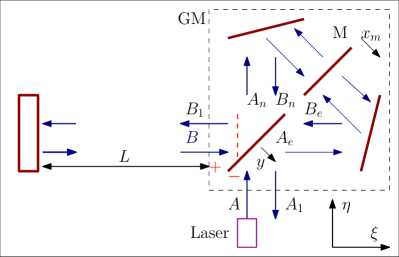
Figure 1: Michelson-Sagnac interferometer as a generalized mirror (GM) of FP cavity. Combined coupling takes place when beam splitter is movable but fixed mirror $M$ ($x_{m}$ — const).

III Examples of realizations of combined coupling

For a realization of the combination of dissipative and dispersive couplings we use the Michelson-Sagnac interferometer (MSI) as one of the mirrors in the FP cavity (see Fig. 1). The MSI consists of the 50/50 beam splitter (BS) and three completely reflecting mirrors. This interferometer can be considered as a generalized mirror having amplitude transmittance $T$ and reflectivity $R$ depending on displacements $z_{m}$ of the mirror $M$ and $y_{BS}$ of BS. So input-output relations have the form (see notation on Fig. 1):

$$\mathcal{A}_{1} =\mathcal{B}T+e^{-ik\sqrt{2}y}\mathcal{A}R,$$ (15a)

$$\mathcal{B}_{1} =\mathcal{A}T-e^{ik\sqrt{2}y}\mathcal{B}R,$$ (15b)

$$R =\cos k\big{(}2z_{m}+\sqrt{2}y\big{)},$$ (15c)

$$T =\sin k\big{(}2z_{m}+\sqrt{2}y\big{)},$$ (15d)

where $\mathcal{A}$ and $\mathcal{B}$ are amplitudes coherent monochromatic fields, $k=\frac{\omega}{c}$ is wave vector.

A detailed analysis of MSI is given in XuerebPRL2011 ; TarabrinPRA2013 ; SawadskyPRL2015 ; 16a1PRAVyMa ; 19a1JPhyBNaVy ; 20PRAKaVy . We assume that the waves passing through BS acquire a phase shift equal to $\frac{\pi}{2}$, and the phases of the waves reflected from BS are determined only by the displacement of the BS itself. We also assume that the spectral frequencies $\Omega$, characterizing the displacements of BS and the moving mirror $M$ are small enough: $\Omega t_{in}\ll 1$, where $t_{in}$ is round trip time of light between BS and mirror $M$. This means that the circulating fields change phase almost instantly at small displacements of BS and $M$. Amplitude transmittance $T$ and reflectivity $R$ of the GM depend only on positions $z_{m}$, $y$.

Below we can designate displacement as

$$y\Rightarrow y_{0}+y,\quad z_{m}\Rightarrow z_{0}+z,$$ (16)

where $z_{0},\ y_{0}$ are the mean constants (to be chosen) and $z,\ y$ are small variables.

Below we consider only a situation of movable beam splitter and the mirror $M$ fixed (that is $z=0$). Then we can expand $R,\ T$ (15) into a series

$$R \simeq R_{0}-T_{0}\,k\sqrt{2}\,y\,,$$ (17a)

$$T \simeq T_{0}+R_{0}\,k\sqrt{2}\,y\,,$$ (17b)

$$R_{0} =\cos k\big{(}2z_{0}+\sqrt{2}\,y_{0}\big{)},\quad T_{0}=\sin k\big{(}2z_{0}+\sqrt{2}y_{0}\big{)},$$

For simplicity we put $y_{0}=0$ below, then only $z_{0}$ defines $T_{0},\ R_{0}$.

The MSI is a part of the FP cavity. The field $B_{1}$ propagates to the end mirror (we consider it is completely reflecting), reflects and comes back to the beam splitter. In the stationary mode of operation fields $B$ and $B_{1}$ have the following coupling

$$\mathcal{B}=\mathcal{B}_{1}e^{i2kL},$$ (18)

where $L$ is the distance between the beam splitter and the end mirror.

Let’s substitute (18) in equations (15)

$$\mathcal{A}_{1} =\mathcal{B}_{1}e^{i2kL}T+e^{-ik\sqrt{2}y}\mathcal{A}R,$$ (19a)

$$\mathcal{B}_{1} =\mathcal{A}T-e^{ik\sqrt{2}y}\mathcal{B}_{1}e^{i2kL}R$$ (19b)

The internal field’s power $I_{0}$ is given by the ratio

$$I_{0}=\frac{T^{2}I}{1+R^{2}+2R\cos 2k\left(L+\frac{y}{\sqrt{2}}\right)}.$$ (20)

Where $I$ is the input field power.

This power achieve a maximum on $e^{2ik(L+y/\sqrt{2})}=-1$ (here and below we assume that $R>0$). We can find the resonant frequency from this equation

$$w_{r}=\frac{\omega_{0}}{1+\frac{y}{\sqrt{2}L}}\simeq\omega_{0}\left(1-\frac{y}{\sqrt{2}L}\right).$$ (21)

Here $\omega_{0}$ is the resonant frequency by $y=0$.

Now let’s find the half bandwidths of the cavity $\gamma_{0}$. Let us assume that the wave vector $k$ in equation (20) is equal to $(\omega_{r}+\gamma)/c$ ($\omega_{r}\gg\gamma$) so that $I_{0}=I_{0\text{max}}/2$. Then we get the following relation for $\gamma$

$$\gamma=\frac{2\left(1-R\right)}{\tau\sqrt{R}}\simeq\frac{T^{2}}{\tau}\simeq\frac{T_{0}^{2}}{\tau}\left(1+\frac{2\sqrt{2}k_{0}R_{0}}{T_{0}}\right).$$ (22)

Here we account that $T_{0}\ll 1$.

Let’s compare equations (21) and (22) with (1). We see that coefficients of dispersive ($\xi$) and dissipative ($\eta$) coupling for the system described above have the following form

$$\gamma_{0}=\frac{T_{0}^{2}}{\tau},\quad\xi=-\frac{1}{\sqrt{2}L},\quad\eta=\frac{2\sqrt{2}k_{0}}{T_{0}}.$$ (23)

In Table 1 we list parameters of the system described above, which can be used in a laboratory experiment.

Another example of realizing combined coupling is given in SawadskyPRL2015 ; SawadskyArxiv2015 . The authors described an optical-mechanical system similar to the one presented above, but the test mass was a partially transmitting mirror M and beam splitter was immobile (see Fig. 1). For this case the input-output relations can be written as follows

$$\mathcal{A}_{1} =i\mathcal{B}\mathbb{T}+\mathcal{A}\mathbb{R}_{\triangleright},$$ (24a)

$$\mathcal{B}_{1} =i\mathcal{A}\mathbb{T}+\mathcal{B}\mathbb{R}_{\triangleleft},$$ (24b)

$$\mathbb{T} =e^{ikl_{+}}r_{M}\sin 2k\delta l,$$ (24c)

$$\mathbb{R}_{\triangleright} =e^{ikl_{+}}\left(r_{M}\cos 2k\delta l-it_{M}\right),$$ (24d)

$$\mathbb{R}_{\triangleleft} =e^{ikl_{+}}\left(r_{M}\cos 2k\delta l+it_{M}\right).$$ (24e)

Here $r_{M}$ and $t_{M}$ are the amplitude reflectivity and transmittance of mirror, $l_{+}$ and $\delta l$ are the sum and difference of the lengths of the MSI arms, respectively. We consider that $\delta l=z_{0}+z$, where $z_{0}$ is a constant, and $z$ is a small displacement, $kz\ll 1$.

Now we can find the coefficients of dispersive $\xi_{1}$ and dissipative $\eta_{1}$ coupling for this optomechanical system by conducting the analysis presented above

$$\gamma_{1}=\frac{r_{M}^{2}T_{1}^{2}}{\tau},\quad\xi_{1}=-\frac{T_{1}t_{M}r_{M}}{L},\quad\eta_{1}=\frac{4k_{0}}{T_{1}}.$$ (25)

Here we assume that $|T_{1}|=|\sin 2kz_{0}|\ll 1$ and find resonant frequency $\omega_{0}$ from $e^{ik\left(2L+l_{+}\right)+i\phi_{0}}=1$, where $\phi_{0}=\arctan\left(t_{M}/r_{M}\right)$.

These examples show that we can choose coupling coefficients $\xi,\ \eta$ within some bounds.

Table 1: Parameters of the optomechanical system

Parameter	Value
Medium amplitude transmittance
of MSI $T_{0}$	0.01
Probe mass $m$	50 g
Pump frequency $\omega_{0}/2\pi$	300 THz
Pump power $I_{0}$	42 mW
Cavity length $L$	1 m
Cavity half bandwidth $\gamma_{0}$	15000 $\text{s}^{-1}$
Coefficient of the dissipative coupling $\eta$	$1.78\times 10^{9}$ $\text{m}^{-1}$
Coefficient of the dispersive coupling $\xi$	$-0,71$ $\text{m}^{-1}$

IV Detecting signal force

We consider an optomechanical system with a combination of both couplings $\xi,\ \eta$ as a signal force detector, assuming that $\xi,\ \eta$ can be varied arbitrary. Let’s find the sensitivity of this measurement.

We assume that quadratures of the output field (12a), (12b) are processed optimally for this purpose. Let’s substitute (14) in equations of quadratures (12a) and (12b):

$$a_{1a}=\frac{(x_{0}^{2}-x^{2})a_{a}-P_{m}x^{2}a_{\phi}-ix^{2}\sqrt{2P_{m}}f_{s}}{(x_{0}^{2}-x^{2})-ix\delta_{m}},$$ (26a)

$$a_{1\phi}=\frac{(x_{0}^{2}-x^{2})a_{\phi}+Q_{m}D^{2}a_{a}-xD\sqrt{2Q_{m}}f_{s}}{(x_{0}^{2}-x^{2})-ix\delta_{m}},$$ (26b)

$$P_{m}=\frac{8\hbar\eta^{2}A^{2}}{m\gamma_{0}^{2}},\quad Q_{m}=\frac{32\hbar\xi^{2}A^{2}}{m\gamma_{0}^{2}},$$ (26c)

$$\delta_{m}=\frac{\delta}{m\gamma_{0}}=D\sqrt{P_{m}Q_{m}},\quad x=\frac{\Omega}{\gamma_{0}},\quad x_{0}=\frac{\Omega_{0}}{\gamma_{0}}$$

$$\Omega_{0}=\sqrt{\frac{\kappa}{m}},,\quad f_{s}=\frac{F_{s}}{\sqrt{2\hbar m\Omega^{2}}},\quad D=\frac{\omega_{0}}{\gamma_{0}}.$$ (26d)

Here $f_{s}$ is the signal force normalized to SQL, $\kappa$ and $\delta$ are given by the equations (14d), $\Omega_{0}$ is the resonant frequency which appears due to the optical rigidity (14d), $D$ is the quality factor of the optical cavity. Here and below we assume that $\xi\eta=-|\xi\eta|$ and

$$\Omega,\,\Omega_{0}\ll\gamma_{0},\quad\text{or}\quad x,\,x_{0}\ll 1$$ (27)

It follows from equations (26) that both quadratures are suitable for detecting the signal force. We use the homodyne detection for the measurement of quadratures, allowing to measure a quadrature

$$a_{1\theta}=a_{1a}\cos\theta+a_{1\phi}\sin\theta,$$ (28)

where $\theta$ is a homodyne angle. Let input field is in coherent state. This means that single-sided power spectral densities (PSD) of quadratures $a_{a}$ and $a_{\phi}$ equal $S_{a}(\Omega)=S_{\phi}(\Omega)=1$ 02a1KiLeMaThVyPRD . Then noise PSD recalculated to $f_{s}$ can be easily derived from (26):

$$S_{f} =S_{a1}+S_{\phi 1},$$ (29a)

$$S_{a1} =\frac{\left(x_{0}^{2}-x^{2}+Q_{m}D^{2}\tan\theta\right)^{2}}{2x^{2}\left(x^{2}P_{m}+D^{2}Q_{m}\tan^{2}\theta\right)},$$ (29b)

$$S_{\phi 1} =\frac{\left((x_{0}^{2}-x^{2})\tan\theta-P_{m}x^{2}\right)^{2}}{2x^{2}\left(x^{2}P_{m}+D^{2}Q_{m}\tan^{2}\theta\right)}.$$ (29c)

Here SQL sensitivity corresponds to $S_{f}=1$. When $\theta=0$ we measure the amplitude quadrature, and when $\theta=\frac{\pi}{2}$ we measure the phase quadrature.

Let’s fix $x=x_{c}$ and find $\tan\theta$ at which equation (29) takes an extreme value. There are two $\tan\theta$ and they have the following form

$$\tan\theta_{1}=-\frac{x_{0}^{2}-x_{c}^{2}}{Q_{m}D^{2}},\quad\tan\theta_{2}=\frac{P_{m}x_{c}^{2}}{x_{0}^{2}-x_{c}^{2}}.$$ (30)

Choosing these homodyne angles we completely cancel the noise determined by one of the quadratures, namely, $S_{a1}^{x=x_{c}}=0$ at $\theta=\theta_{1}$ and $S_{\phi 1}^{x=x_{c}}=0$ at $\theta=\theta_{2}$.

Let’s consider a special case $x_{c}=x_{0}$. Then $\tan\theta_{1}=0$ and $\tan\theta_{2}=\pm\infty$. This means that we measure the quadrature of the amplitude or phase. In these measurements PSDs have the following form

$$S_{f}|^{\theta=0}=\frac{1}{2}\left[P_{m}+\frac{\left(\left(\frac{x_{0}}{x}\right)^{2}-1\right)^{2}}{P_{m}}\right],$$ (31a)

$$S_{f}|^{\theta=\frac{\pi}{2}}=\frac{1}{2x^{2}}\left[Q_{m}D^{2}+\frac{(x_{0}^{2}-x^{2})^{2}}{Q_{m}D^{2}}\right].$$ (31b)

In resonance case $\Omega=\Omega_{0}$

$$S_{f}(\Omega_{0})|^{\theta=0} =\frac{P_{m}}{2}=x_{0}^{2}g,\quad g=\sqrt{\frac{P_{m}}{Q_{m}D^{2}}}$$ (32a)

$$S_{f}(\Omega_{0})|^{\theta=\pi/2} =\frac{D^{2}Q_{m}}{2x_{0}^{2}}=\frac{1}{g}.$$ (32b)

Here we rewrite the PSD using equations (26c) and (26), $g$ is a ratio between coefficients of optomechanical couplings.

The relations (32) show that at $g\ll 1/\sqrt{x_{0}}$ we have inequality $S_{f}(\Omega_{0})|^{\theta=0}\ll S_{f}(\Omega_{0})|^{\theta=\pi/2}$ and in order to surpass SQL near the resonant frequency we have to detect amplitude quadrature (i.e., $\theta=0$). In the opposite case $g\gg 1/\sqrt{x_{0}}$ we have inverse inequality $S_{f}(\Omega_{0})|^{\theta=0}\ll S_{f}(\Omega_{0})|^{\theta=\pi/2}$ and to surpass SQL one has to detect the phase quadrature (i.e., $\theta=\pi/2$).

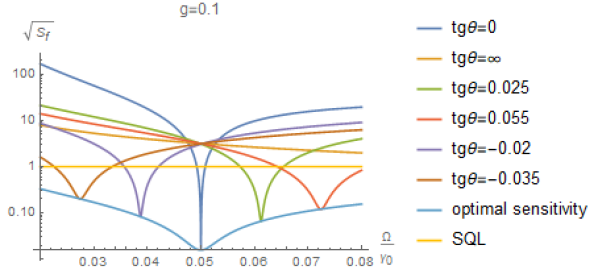
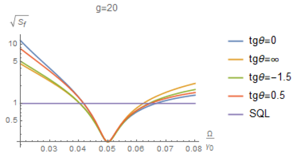
Figure 2: Graphs of amplitude spectral densities $\sqrt{S_{f}(\Omega)}$ plotted for the homodyne detection having different homodyne angles and ratio $g$ and fixed dimensionless frequency $x_{0}=0.05$. The upper graphs are obtained for $g=0.1$ The middle graphs correspond to condition (33) $g=1/x_{0}=20$. The graphs at the bottom are plotted for the case $g=400\gg 1/x_{0}$. Also upper and bottom graphs show the optimal PSD by the optimal frequency-dependent homodyne angle (see in Appendix A).

Recall, $S_{f}(\Omega_{0})|^{\theta=0}$ and $S_{f}(\Omega_{0})|^{\theta=\pi/2}$ are extremes of one function. The maximum (minimim) depends on ratio $g$. However, at $g=1/x_{0}$ they became equal to each other (the maximum and the minimum coincide):

$$S_{f}(\Omega_{0})|^{\theta=0} =S_{f}(\Omega_{0})|^{\theta=\pi/2}=x_{0},\quad\text{at }g=\frac{1}{x_{0}}$$ (33)

Thus, when $g=1/x_{0}$ we get the same sensitivity near the resonant frequency for any quadrature detection. Usually $x_{0}\ll 1$ (the case of non-resolved sideband), hence, SQL can be surpassed.

The minimum PSD is achieved at the resonant frequency and it is defined by equations (32) . This minimum PSD is realized inside a narrow bandwidth $\Gamma$:

$$\frac{\Gamma}{\Omega_{0}}\simeq S_{f}^{\text{min}}.$$ (34)

Here $\Gamma$ is defined as $S_{f}(\Omega_{0}\pm\Gamma/2)\simeq 2S_{f}^{\text{min}}$. The relation (34) corresponds to the known Cramer-Rao bound Mizuno ; Mizuno93 ; Miao2017 .

In Fig. 2 we depict graphs of amplitude spectral densities $\sqrt{S_{f}(\Omega)}$ of noise recalculated to $f_{s}$ by the homodyne detection with different homodyne angles and ratio $g$ and fixed dimensionless frequency $x_{0}=0.05$ and pump power (so $|\xi\eta|=1$). The main parameters (test mass, optical power) are taken from Table 1 with varying coupling $\xi,\ \eta$. The plots are given for preliminary chosen fixed homodyne angle. For methodical purpose on upper and bottom graphs we also show the optimal PSD by the optimal frequency-dependent homodyne angle (see in Appendix A).

The upper graphs in Fig. 2 are obtained for $g=0.1$. Varying homodyne angle one can surpass SQL at frequencies close to mechanical resonance. At mechanical resonance the sensitivity attains the minimum but in narrow bandwidth. SQL can be surpassed when the frequency differs from the resonance one by about 50%, but sensitivity will by slightly drop and the bandwidth will be wider if compared to the case of mechanical resonance.

The middle graphs in Fig. 2 correspond to condition (33) $g=1/x_{0}=20$. SQL can be surpassed within a relatively wider bandwidth (about 50% of center frequency). Variation of homodyne angle practically does not influence on sensitivity.

And the bottom graphs in Fig. 2 describe the case $g=400\gg 1/x_{0}$. Variation of homodyne angle allows surpassing SQL inside the bandwidths close to the mechanical resonance. It is similar to the case shown in upper graphs.

Above we assumed that $\xi,\ \eta$ can be varied arbitrary. But usually these coefficients are constant in certain systems. For example, the Fabry-Perot cavity with the MSI with the movable BS has fixed $\xi$ and $\eta$ (see (23)), and the ratio $g=T_{0}\ll 1$.

If only the partially transmitting mirror M is movable in the MSI, then coefficients (25) are constant too, and $g=r_{M}/t_{M}$. In this case we can get an optomechanical system with a large coefficient $g$ if $r_{M}\gg t_{M}$.

V Ponderomotive squeezing

We would like to pay attention to the fact that combined optomechanical coupling can also be used to produce a pondermotive squeezed light. In turn, varying ratio $g$ (32a) between dispersive and dissipative coupling provides for a possibility to control output squeezing. The output quadrature (28) measured by homodyne detector can be derived from (26):

$$a_{1\theta} =\frac{(x_{0}^{2}-x^{2})\cos\theta+\frac{2x_{0}^{2}}{g}\sin\theta}{\left(x_{0}^{2}-x^{2}\right)-2ixx_{0}^{2}}\,a_{a}+$$ (35a)

$$\quad+\frac{\left(x_{0}^{2}-x^{2}\right)\sin\theta-2x_{0}^{2}x^{2}g\cos\theta}{\left(x_{0}^{2}-x^{2}\right)-2ixx_{0}^{2}}\,a_{\phi}$$ (35b)

In the case of the mechanical resonance $\Omega=\Omega_{0}$ this equation can be written as follows:

$$a_{\theta}|_{x=x_{0}}=\frac{i}{gx_{0}}\sin\theta\,a_{a}-ix_{0}g\cos\theta\,a_{\phi};$$ (36)

Obviously, in order to measure squeezing for small $g\ll 1/x_{0}$ one has to choose $\sin\theta=0$ and to measure amplitude output quadrature. In contrast, to measure squeezing for large $g\gg 1/x_{0}$ one has to choose $\cos\theta=0$ and to measure the phase output quadrature (see (40) in Appendix A):

$$S_{a}(\Omega_{0}) =x_{0}^{2}g^{2},\quad(\sin\theta=0)$$ (37a)

$$S_{\phi}(\Omega_{0}) =\frac{1}{g^{2}x_{0}^{2}},\quad(\cos\theta=0),$$ (37b)

where $S_{a}$ and $S_{\phi}$ are single-sided PSD of output amplitude and phase quadratures, respectively, and we assume that condition (27) is valid. Such squeezing near the resonant frequency $\Omega_{0}$ is not observed in the case of dispersion coupling.

In case (33) $g=1/x_{0}$ the output light is practically coherent and it is required to pay attention to scale on vertical axis of middle plots on Fig. 3.

Specifically, in the case of low frequencies $\Omega\ll\Omega_{0}$ ($x\ll x_{0}$) we get frequency-independent squeezing:

$$\Omega\ll\Omega_{0}\quad g\ll 1:\ S_{\theta}^{\text{comb}}\simeq\frac{g^{2}}{4},$$ (38)

here $S_{\theta}^{\text{comb}}$ is a single-sided PSD of the output quadrature (28) at optimal homodyne angle in case of combined coupling (see details in Appendix A).

It is similar to what we obtained in the case of the dispersive coupling with a non-resonant pump ($\Delta=\omega_{p}-\omega_{0}$ is detuning) 06PRAcckovwm :

$$\Omega\ll\Omega_{0},\quad\frac{\Delta}{\gamma_{0}}\ll 1:\ S_{\theta}^{\text{disper}}\simeq\frac{\Delta^{2}}{\gamma_{0}^{2}},$$ (39)

where $S_{\theta}^{\text{disper}}$ are single-sided PSD of output quadrature (28) at optimal homodyne angle for dispersive coupling. The PSD (38, 39) are equal to each other when $\frac{g}{2}=\frac{\Delta}{\gamma_{0}}$ and practically do not depend on the frequency.

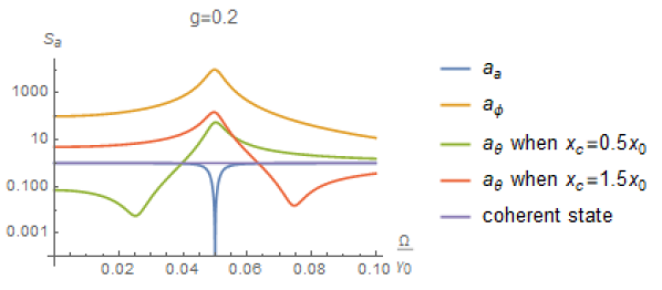
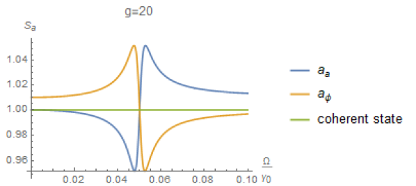
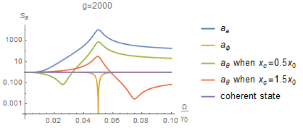
Figure 3: Graphs of single-sided PSD of different quadratures by different parameter $g$ and the fixed resonant frequency $x_{0}=0.05$. The upper graphs are constructed for $g=0.2\ll 1/x_{0}$. The middle graphs are constructed for $g=1/x_{0}=20$, here we get an almost coherent state of the electromagnetic field (pay attention to scale on vertical axis). And bottom graphs relate to case $g=2000\gg 1/x_{0}$.

In general case we can adjust the maximum squeezing at preliminary chosen dimensionless frequency $x_{c}$ (near $x_{0}$) by varying homodyne angle $\theta$ at a fixed ratio $g$ (see details of calculations in Appendix A). If compared with dispersive case the main advantage of combined coupling deals with possibility to vary degree of squeezing and its bandwidth choosing $x_{c}$ (i.e., the homodyne angle).

Shown in Fig. 3 are the plots of single-sided PSD (41c) obtained for the output light for normalized mechanical frequency $x_{0}=0.05$ when $x_{c}=0.5x_{0}$ or $x_{c}=1.5x_{0}$ and different ratio $g$. For $g=1/x_{0}$ (the middle plot in Fig. 3) the output state is practically coherent at $\Omega=\Omega_{0}$ but out of resonance in case of squeezing. But the farther $g$ is from $1/x_{0}$, the stronger the squeezing becomes near $x_{0}$. For small $g\ll 1/x_{0}$ we get the amplitude quadrature squeezed near the resonance, and for large $g\gg 1/x_{0}$ the phase quadrature. It is possible to get less strong squeezing but in a wider frequency band at other frequencies. This can be done measuring a quadrature $a_{1\theta}$ other than the amplitude and phase.

VI Discussion and conclusion

We analysed the optomechanical system, featuring combination of dispersive and dissipative coupling, and showed that the main properties of combined coupling deal with the optical rigidity (14), which appears as a result of both kinds of coupling. At the same time, this rigidity manifests in systems having combined coupling on the resonant pump, which is not typical for pure dispersive 06PRAcckovwm or dissipative 16a1PRAVyMa coupling types.

For realizing the combination of dissipative and dispersive coupling we used the MSI as an input mirror in the FP cavity (see Fig. 1). We considered two different modes of operation of the MSI with a movable beam splitter and an immobile completely reflecting mirror M and vice versa with a movable partially transmitting mirror M and a fixed beam splitter. The coefficients of the dispersive $\xi$ and dissipative $\eta$ coupling for these schemes were obtained. In further analysis, we assumed that $\xi$ and $\eta$ can be varied arbitrary.

We considered an optomechanical system with a combination of both couplings as a signal force detector. Homodyne detection of an output field can have a sensitivity better than SQL near the resonant frequency $\Omega_{0}$, which is defined by the optical rigidity (14d). The analysis shows that it is most effective to measure the amplitude or phase quadrature (the choice of the quadrature depends on the ratio $g$ as compared with $1/x_{0}$ (33)). If $g<1/x_{0}$, it is better to measure the amplitude quadrature, and if $g>1/x_{0}$ — the phase quadrature. At $g=1/x_{0}$ we get the same sensitivity near the resonant frequency for measuring any quadrature. In this case the PSD recalculated to force SQL (33) is smaller than unity (i.e. SQL can be surpassed) if $x_{0}=\Omega_{0}/\gamma_{0}\ll 1$.

The physical reason is related to the correlation between the measurement noise and the fluctuation back action. This correlation occurs due to the combination of both optomechanical couplings. Indeed, the fluctuation back action force (14b) depends on the phase quadrature (dissipative coupling) and on the amplitude quadrature (dispersive coupling) and the measurement noise is determined by the amplitude or phase quadrature (first terms in Eq. 12a and 12b). Part of the total noise is completely compensated at the resonant frequency (see Eq. 26). The remaining noise recalculated to $f_{s}$ is proportional to $\sqrt{P_{m}}$ or $\sqrt{D^{2}Q_{m}}/x_{0}$, depending on which quadrature we measure. SQL is surpassed if this noise is small.

We would like to point out that variation of ratio $g$ between dispersive and dissipative coupling and choice of homodyne angle provide possibility to control output poderomotive squeezing. Varying homodyne angle we can obtain constant squeezing at frequencies much smaller than resonant frequency $\Omega_{0}$, or large squeezing in finite bandwidth (the larger squeezing, the more narrow bandwidth) near the resonant frequency. The ponderomotive squeezing induced by combined coupling has a wider range of varying squeezing parameters as compared with ponderomotive squeezing caused by dispersive coupling.

The combined coupling looks promising to be used in gravitational wave antennas for creation of frequency dependent squeezing with controllable parameters. The main obstacle is thermal mechanical noise. It is the subject of our future research.

Appendix A The analysis of the pondermotive squeezing.

From (35) one can calculate single-sided PSD assuming coherent input light

$$S_{\theta} =\frac{\left(x_{0}^{2}-x^{2}\right)^{2}+4x_{0}^{4}\left(\frac{\sin^{2}\theta}{g^{2}}+x^{4}g^{2}\cos^{2}\theta\right)}{\left(x_{0}^{2}-x^{2}\right)^{2}+4x^{2}x_{0}^{4}}+$$ (40a)

$$\quad+\frac{4x_{0}^{2}\left(x_{0}^{2}-x^{2}\right)\sin\theta\cos\theta\left(\frac{1}{g}-x^{2}g\right)}{\left(x_{0}^{2}-x^{2}\right)^{2}+4x^{2}x_{0}^{4}}=$$ (40b)

$$=\frac{W+U\cos 2\theta+V\sin 2\theta}{\left(x_{0}^{2}-x^{2}\right)^{2}+4x^{2}x_{0}^{4}}$$ (40c)

$$W =\left(x_{0}^{2}-x^{2}\right)^{2}+\frac{2x_{0}^{4}}{g^{2}}+2x^{4}x_{0}^{4}g^{2},$$ (40d)

$$U =2x_{0}^{2}\left[x^{4}x_{0}^{2}g^{2}-\frac{x_{0}^{2}}{g^{2}}\right],$$ (40e)

$$V =2x_{0}^{2}\left(x_{0}^{2}-x^{2}\right)\left[\frac{1}{g}-x^{2}g\right]$$ (40f)

The minimum of $S_{\theta}$ at $x=x_{c}$ takes place at homodyne angle $\theta$ defined as

$$\cos 2\theta =-\frac{U_{c}}{\sqrt{U_{c}^{2}+V_{c}^{2}}},\quad\sin 2\theta=-\frac{V_{c}}{\sqrt{U_{c}^{2}+V_{c}^{2}}},$$ (41a)

$$U_{c} =U|_{x=x_{c}},\quad V_{c}=V|_{x=x_{c}}.$$ (41b)

and it is equal to

$$S_{\theta}^{x_{c}}(x) =\frac{W-\frac{UU_{c}+VV_{c}}{\sqrt{U_{c}^{2}+V_{c}^{2}}}}{\left(x_{0}^{2}-x^{2}\right)^{2}+4x^{2}x_{0}^{4}}$$ (41c)

In particular case $x\ll x_{0}$ we have

$$W \simeq x_{0}^{4}\left(1+\frac{2}{g^{2}}\right),\quad U\simeq-\frac{2x_{0}^{4}}{g^{2}},\quad V\simeq\frac{2x_{0}^{4}}{g},$$ (42a)

$$S_{\theta} {}^{x\ll x_{0}}\simeq 1+\frac{2}{g^{2}}-\frac{2}{g^{2}}\cos 2\theta+\frac{2}{g}\sin 2\theta\geq$$ (42b)

$$\geq\frac{\sqrt{1+g^{2}}-1}{\sqrt{1+g^{2}}+1}=\frac{g^{2}}{4}-\frac{g^{4}}{8}+\dots$$ (42c)

References

- (1) LVC-Collaboration, “Prospects for Observing and Localizing Gravitational-Wave Transients with Advanced LIGO and Advanced Virgo,” arXiv, vol. 1304.0670, 2013.
- (2) J. Aasi et al (LIGO Scientific Collaboration) et al., “Advanced LIGO,” Classical and Quantum Gravity, vol. 32, p. 074001, 2015.
- (3) D. Martynov et al., “Sensitivity of the Advanced LIGO detectors at the beginning of gravitational wave astronomy,” Physical Review D, vol. 93, p. 112004, 2016.
- (4) F. Asernese et al., “Advanced Virgo: a 2nd generation interferometric gravitational wave detector,” Classical and Quantum Gravity, vol. 32, p. 024001, 2015.
- (5) K. L. Dooley, J. R. Leong, T. Adams, C. Affeldt, A. Bisht, C. Bogan, J. Degallaix, C. Graf, S. Hild, and J. Hough, “GEO 600 and the GEO-HF upgrade program: successes and challenges,” Classical and Quantum Gravity, vol. 33, p. 075009, 2016.
- (6) Y. Aso, Y. Michimura, K. Somiya, M. Ando, O. Miyakawa, T. Sekiguchi, D. Tatsumi, and H. Yamamoto, “Interferometer design of the KAGRA gravitational wave detector,” Physical Review D, vol. 88, p. 043007, 2013.
- (7) S. Forstner and S. Prams and J. Knittel and E.D. van Ooijen and J.D. Swaim and G.I. Harris and A. Szorkovszky and W.P. Bowen and H. Rubinsztein-Dunlop, “Cavity Optomechanical Magnetometer,” Physical Review Letters, vol. 108, p. 120801, 2012.
- (8) B.-B. Li, J. Bílek, U. Hoff, L. Madsen, S. Forstner, V. Prakash, C. Schafermeier, T. Gehring, W. Bowen, and U. Andersen, “Quantum enhanced optomechanical magnetometry,” Optica, vol. 5, p. 850, 2018.
- (9) M. Wu, A.C. Hryciw, C. Healey, D.P. Lake, H. Jayakumar, M.R. Freeman, J.P. Davis, and P.E. Barclay, “Dissipative and dispersive optomechanics in a nanocavity torque sensor,” Physical Review X, vol. 4, p. 021052, 2014.
- (10) P. H. Kim, B. D. Hauer, C. Doolin, F. Souris, and J. P. Davis, “Approaching the standard quantum limit of mechanical torque sensing,” Nature Communications, vol. 7, p. 13165, 2016.
- (11) J. Ahn, Z. Xu, J. Bang, P. Ju, X. Gao, and T. Li, “Ultrasensitive torque detection with an optically levitated nanorotor,” Nature Nanotechnoligy, vol. 15, p. 89–93, 2020.
- (12) V.B. Braginsky, “Classic and quantum limits for detection of weak force on acting on macroscopic oscillator,” Sov. Phys. JETP, vol. 26, p. 831–834, 1968.
- (13) V.B. Braginsky and F.Ya. Khalili, Quantum Measurement. Cambridge University Press, Cambridge, 1992.
- (14) H.J. Kimble, Y. Levin, A.B. Matsko, K.S. Thorne, and S.P. Vyatchanin, “Conversion of conventional gravitational-wave interferometers into QND interferometers by modifying input and/or output optics,” Phys. Rev. D, vol. 65, p. 022002, 2001.
- (15) T. Kippenberg and K. Vahala, “Cavity Optomechanics: Back Action at the Mesoscale,” Science, vol. 321, p. 1172–1176, 2008.
- (16) J.M. Dobrindt and T.J. Kippenberg, “Theoretical Analysis of Mechanical Displacement Measurement Using a Multiple Cavity Mode Transducer ,” Physical Review Letters, vol. 104, p. 033901, 2010.
- (17) S.P. Vyatchanin and A.B. Matsko, “Quantum limit of force measurement,” Sov.Phys – JETP, vol. 77, p. 218–221, 1993.
- (18) S. Vyatchanin and E. Zubova, “Quantum variation measurement of force,” Physics Letters A, vol. 201, p. 269–274, 1995.
- (19) The LIGO Scientific collaboration, “A gravitational wave observatory operating beyond the quantum shot-noise limit,” Nature Physics, vol. 73, p. 962–965, 2011.
- (20) LIGO Scientific Collaboration and Virgo Collaboration, “Enhanced sensitivity of the LIGO gravitational wave detector by using squeezed states of light,” Nature Photonics, vol. 7, p. 613–619, 2013.
- (21) V. Tse et al., “Quantum-Enhanced Advanced LIGO Detectors in the Era of Gravitational-Wave Astronomy,” Physical Review Letters, vol. 123, p. 231107, 2019.
- (22) F. Asernese, et al, and (Virgo Collaboration), “Increasing the Astrophysical Reach of the Advanced Virgo Detector via the Application of Squeezed Vacuum States of Light,” Physical Review Letters, vol. 123, p. 231108, 2019.
- (23) M. Yap, J. Cripe, G. Mansell, et al., “Broadband reduction of quantum radiation pressure noise via squeezed light injection,” Nature Photonics, vol. 14, p. 19–23, 2020.
- (24) H. Yu et al., “Quantum correlations between the light and kilogram-mass mirrors of LIGO,” arXive, vol. 2002.01519, 2020.
- (25) J. Cripe, N. Aggarwal, R. Lanza, et al., “Measurement of quantum back action in the audio band at room temperature,” Nature, vol. 568, p. 364–367, 2019.
- (26) V.B. Braginsky and F.Ya. Khalili., “Gravitational wave antenna with QND speed meter,” Physics Letters A, vol. 147, p. 251–256, 1990.
- (27) V.B. Braginsky, M.L. Gorodetsky, F.Y. Khalili, and K.S. Thorne, “Dual-resonator speed meter for a free test mass,” Physical Review D, vol. 61, p. 044002, 2000.
- (28) V.B. Braginsky and F.Ya. Khalili, “Low noise rigidity in quantum measurements,” Phys. Lett. A, vol. 257, p. 241, 1999.
- (29) F.Ya. Khalili, “Frequency-dependent rigidity in large-scale interferometric gravitational-wave detectors,” Physics Letters A, vol. 288, p. 251–256, 2001.
- (30) M. Tsang and C. Caves, “Coherent Quantum-Noise Cancellation for Optomechanical Sensors,” Phys. Rev. Lett., vol. 105, p. 123601, 2010.
- (31) E. Polzik and K. Hammerer, “Trajectories without quantum uncertainties,” Annalen de Physik, vol. 527, p. A15–A20, 2014.
- (32) C. Moller, R. Thomas, G. Vasilakis, E. Zeuthen, Y. Tsaturyan, M. Balabas, K. Jensen, A. Schliesser, K. Hammerer, and E. Polzik, “Quantum back-action-evading measurement of motion in a negative mass reference frame,” Nature, vol. 547, p. 191–195, 2017.
- (33) F. Elste and S.M. Girvin and A.A. Clerk, “Quantum noise interference and backaction cooling in cavity nanomechanics,” Physical Review Letters, vol. 102, p. 207209, 2009.
- (34) M. Li and W.H.P. Pernice and H.X. Tang, “Reactive cavity optical force on microdisk-coupled nanomechanical beam waveguides,” Physical Review Letters, vol. 103, p. 223901, 2009.
- (35) T. Weiss, C. Bruder, and A. Nunnenkamp, “Strong-coupling effects in dissipatively coupled optomechanical systems,” New Journal of Physics, vol. 15, p. 045017, 2013.
- (36) A. Hryciw, M. Wu, B. Khanaliloo, and P. Barclay, “Tuning of nanocavity optomechanical coupling using a near-field fiber probe,” Optica, vol. 2, no. 5, p. 491, 2015.
- (37) A. Xuereb, R. Schnabel, and K. Hammerer, “Dissipative Optomechanics in a Michelson-Sagnac Interferometer,” Physical Review Letters, vol. 107, p. 213604, 2011.
- (38) S. Tarabrin, H. Kaufer, F. Khalili, R. Schnabel, and K. Hammerer, “Anomalous dynamic backaction in interferometers,” Physical Review A, vol. 88, p. 023809, 2013.
- (39) A. Sawadsky, H. Kaufer, R. Nia, S. Tarabrin, F. Khalili, K. Hammerer, and R. Schnabel, “Observation of generalized optomechanical coupling and cooling on cavity resonance,” Physical Review Letters, vol. 114, p. 043601, 2015.
- (40) S.P. Vyatchanin and A.B. Matsko, “Quantum speed meter based on dissipative coupling,” Physical Review A, vol. 93, p. 063817, 2016.
- (41) A. Nazmiev and S. Vyatchhanin, “Stable optical rigidity based on dissipative coupling,” J. Phys. B: At. Mol. Opt. Phys., vol. 52, p. 155401, 2019.
- (42) A. Karpenko and S. Vyatchanin, “Dissipative coupling, dispersive coupling, and their combination in cavityless optomechanical systems,” Physical Review A, vol. 102, p. 023513, 2020.
- (43) S. Huang and G.S. Agarwal, “Reactive-coupling-induced normal mode splittings in microdisk resonators coupled to waveguides,” Physical Review A, vol. 81, p. 053810, 2010.
- (44) S. Huang and G.S. Agarwal, “Reactive coupling can beat the motional quantum limit of nanowaveguides coupled to a microdisk resonator,” Physical Review A, vol. 82, p. 033811, 2010.
- (45) D. Walls and G. Milburn, Quantum optics. Springer-V Berlin Heidelbergerlag, 2008.
- (46) T. Corbit, Y. Chen, F. Khalili, D. Ottoway, S. Vyatchanin, S. Whitcomb, and N. Mavalvala, “Squeezed-state source using radiation-pressure-induced rigidity,” Physical Review A, vol. 73, p. 023801, 2006.
- (47) A. Sawadsky, H. Kaufer, R. M. Nia, S. P. Tarabrin, F. Y. Khalili, K. Hammerer, and R. Schnabel, “Observation of Generalized Optomechanical Coupling and Cooling on Cavity Resonance,” arXiv, vol. 1409.3398, 2015.
- (48) J. Mizuno, Comparison of optical configuration for laser interferometric gravitational wave detectors. PhD thesis, 1996.
- (49) J. Mizuno, K. Strain, P. Nelson, J. Chen, R. Schilling, A. Rüdiger, W. Winkler, and K. Danzmann Physics Letters A, vol. 175, p. 273, 1993.
- (50) H. Miao, R. Adhikari, Y. Ma, B. Pang, and Y. Chen, “Towards the Fundamental Quantum Limit of Linear Measurements of Classical Signals,” Physical Review Letters, vol. 119, p. 050801, 2017.