Universal Properties of Weakly Bound Two-Neutron Halo Nuclei
Masaru Hongo
Department of Physics, University of Illinois, Chicago, Illinois 60607, USA
RIKEN iTHEMS, RIKEN, Wako 351-0198, Japan
Department of Physics, Niigata University, Niigata 950-2181, Japan
Dam Thanh Son
Kadanoff Center for Theoretical Physics, University of Chicago, Chicago, Illinois 60637, USA
(January 2022)
Abstract
We construct an effective field theory of a two-neutron halo nucleus
in the limit where the two-neutron separation energy and the
neutron-neutron two-body virtual energy are smaller than
any other energy scale in the problem, but the scattering between the
core and a single neutron is not fine-tuned, and the Efimov effect
does not operate. The theory has one dimensionless coupling which
formally runs to a Landau pole in the ultraviolet. We show that many
properties of the system are universal in the double fine-tuning
limit. The ratio of the mean-square matter radius and charge radius
is found to be , where is
the mass number of the core and is a function of the ratio
which we find explicitly. In particular, when
, . The shape of
the dipole strength function also depends only on the ratio
and is derived in explicit analytic form. We estimate
that for the 22C nucleus higher-order corrections to our theory
are of the order of 20% or less if the two-neutron separation energy is less
than 100 keV and the -wave scattering length between a neutron and
a 20C nucleus is less than 2.8 fm.
Introduction.—Neutron-rich nuclei near the neutron drip line
are at the forefront of modern nuclear physics. Some of the most
exotic examples are two-neutron halo nuclei, consisting of a
relatively tightly bound core and two weakly bound neutrons, e.g.,
6He, 11Li, and 22C. These nuclei are called
“Borromean,” i.e., bound states of three objects which would fall
apart when one is removed [1].
In this Letter, we develop an effective field theory (EFT) that can
describe Borromean two-neutron halo nuclei in the limit of very small
two-neutron separation energy . The impetus to the construction of
this theory is the observation of the halo nucleus 22C with a
matter radius found to be as large as 5.4(9) fm [2]
which requires a small : keV [3]. A
later experiment [4] yields a smaller matter radius—3.44(8) fm—relaxing the upper limit to keV, but if one
incorporates the information about the neutron-core
scattering [5], the upper limit is reduced to
keV [6]. So 22C is likely the least
bound among the known Borromean nuclei.
Our EFT requires two fine-tunings: We assume that the neutron-neutron
-wave scattering length is unnaturally large and the
two-neutron separation energy of the halo nucleus is unnaturally
small. In other words, the - two-body virtual energy
keV (here, is the
neutron mass) and the binding energy of the core with two neutrons
are assumed to be smaller than all other energy scales in the problem.
We do not presume any hierarchy between these two energies.
Some previous attempts to apply the EFT philosophy to two-neutron halo
nuclei [7, 6] rely on the existence of a
near-threshold resonance in the core-neutron subsystem and the
three-body Efimov effect [8]. This resonance seems
to be absent in the case of 22C, where experiment points to a
rather small scattering length [5].
The theory developed in this Letter is designed to address this
situation. It may also be a reasonable starting point for a
description of the 3He4He2 molecular trimer [9],
whose binding energy
(– mK) 111See, e.g.,
Ref. [28]
for a compilation of theoretical
predictions.
is somewhat smaller than the energy scale set by the
– scattering length (around
50 mK [11]).
The EFT, to be described, contains two relevant parameters and one
dimensionless coupling. The two relevant parameters correspond to the
two fine-tunings. The dimensionless coupling can be interpreted
as the probability that a halo nucleus splits into a core and a
two-neutron dimer (“dineutron”), and it runs logarithmically with
energy, reaching formally a Landau pole in the ultraviolet (UV) and
zero in the infrared (IR) 222In practice, the running is
limited in the UV by the UV cutoff and in the IR by or ,
whichever is larger.. All other coupling constants are irrelevant
and can be neglected in leading-order calculation.
Using the EFT, one can compute many physical quantities. In particular,
we compute the ratio of the mean-square matter radius and charge
radius. The result is particularly simple in the limit of infinite
neutron-neutron scattering length:
(1)
where is the mass number of the core. We also obtain a fully
analytic expression for the dipole strength function,
Eqs. (29) and (30).
All calculations in this Letter are performed under the assumption
that the core and the neutron are pointlike particles. To translate
our results to the realistic nuclei, one needs account for the charge
and matter distribution inside the core and the neutrons. In
addition, effects from irrelevant terms in the effective Lagrangian
may need to be taken into account.
The effective field theory.—We first write down the effective
Lagrangian for the neutron sector. Denoting the neutron by
, being the spin index,
(2)
From now on, we set . Using a
Hubbard-Stratonovich transformation, the Lagrangian can be transformed
into
(3)
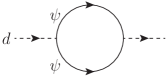
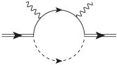
Figure 1: The self-energy of the dimer.
Computing the self-energy of the dimer , which, in the
nonrelativistic theory, is exactly given by the one-loop diagram in
Fig. 1, we find the full dimer propagator
(4)
where denotes the -wave scattering length given by
(5)
The integral on the right-hand side linearly diverges in the UV and is
proportional to the UV cutoff. The fine-tuning of leads to an
unnaturally large scattering length . Note that the UV behavior of
the dimer propagator is different from that of a free field. In fact,
the UV behavior corresponds to a field of dimension 2:
[13] 333In our convention, the dimension of
momentum is 1 and energy is 2..
To construct the EFT describing the halo nucleus, we add into the
theory a field describing the core and describing the halo
nucleus. They can be either bosonic or fermionic.
The effective Lagrangian is now 444This Lagrangian was, in essence,
previously considered in Ref. [29] for the case of a
three-body resonance, i.e., when the three-body binding
energy is negative.
(6)
where and are the masses of the core and
the halo nucleus, respectively. As and
, the dimension of the interaction is 5, which means that is dimensionless. One can check that
terms not included in Eq. (6) are all irrelevant, since they are accompanied by more fields or derivatives. One can
compute the beta function for [16]:
(7)
The solution to this equation is
(8)
where is the energy of the Landau pole.
Because of the properties of the nonrelativistic theory, our subsequent
calculations can be done to all orders in .
One can arrive at the effective Lagrangian (6) by starting
from a theory where the core and the resonantly interacting
neutron are coupled to each other by a contact interaction
, with a UV cutoff at the Landau pole scale.
Through a Hubbard-Stratonovich transformation, one introduces an
auxiliary field with the coupling .
Integrating out degrees of freedom in a energy shell between and
, one generates a kinetic term for and arrive
to Eq. (6) 555In this scenario, the halo nucleus is bound
by the three-body force. One should note, however, that the effective
Lagrangian is valid irrespective of the nature of the microscopic
force responsible for the binding of the halo nucleus..
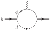
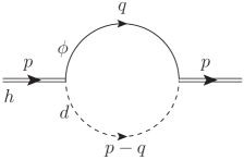
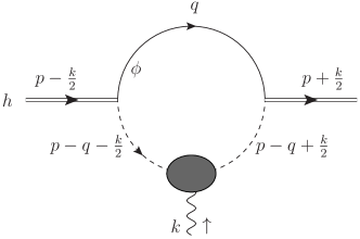
Figure 2: The Feynman diagram determining the charge form factor of
the halo nucleus. The double line represents the halo nucleus, the
single line—the core, and the dotted line—the neutron dimer, whose
propagator is given in Eq. (4).
Charge and matter radii.—We now proceed to extract physical
observables from the Lagrangian (6). The mean-square (rms)
charge radius (the rms of the deviation of the coordinates of the core
from the center of mass 666What we call here the mean-square
charge radius should be understood, for real nuclei, as the difference
between the mean-square point-proton radii of the halo and core
nuclei. Similarly, what is later called the mean-square matter radius
is for real nuclei , where
and are the mean-square matter radii of
the halo and the core, respectively.)
can be extracted from the electric
form factor of the halo nucleus: [recall that is a Fourier transform of the charge density].
The electric form factor is given by the Feynman diagram in
Fig. 2; it is proportional to
, and by dimensional analysis one should have , where we introduce the dimensionless parameter
(9)
where (we assume ).
Computing the Feynman diagram [16], we find 777In subsequent
formulas, is the renormalized coupling in the on-shell
renormalization scheme.
(10)
where
(11)
One can further define the “neutron radius” by imagining that there
is a U(1) gauge boson coupled to the neutrons outside the
core 888This can be done by coupling a gauge field to , where is the baryon charge, is the electric charge, and
and are the atomic and mass numbers, respectively, of the core.
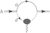
, which describes the spatial size of the dineutron distribution. The
Feynman diagram determining the form factor of the halo nucleus with
respect to this “neutron-number photon” is drawn in
Fig. 3, where the effective coupling of the dimer
to the photon is as in Fig. 4.
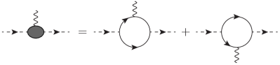
Figure 3: The Feynman diagram determining the “neutron form factor”
of the halo nucleus.Figure 4: The effective vertex of the dimer-photon coupling.
Both and are continuous at and
have the following asymptotics at small and large values of the
argument:
(14)
(15)
From the charge radius and the neutron radius one can compute other
radii—the mean-square matter radius , the neutron-neutron
distance , and the core-neutron distance
999
Using the positions of the core and two neutrons and ,
we define
,
, and
.:
(16)
(17)
(18)
When is fixed, these radii depend on in the following
way. When , the coupling is set at the scale ,
and . When , is
frozen at the scale , and the radii grow logarithmically
as : , which is a known
result [22].
Note that, due to the running of the coupling , the results for the
radii are not truly “universal”: They cannot be expressed solely in
terms of low-energy observables—the three-body binding energy
and the neutron-neutron scattering length . Instead, they depend
logarithmically on the UV cutoff through the coupling . However,
the dependence on disappears when one computes the ratios
of the radii. For example, the ratio of the rms matter and charge
radii is
(19)
while the ratio of the core-neutron and neutron-neutron distances is
(20)
In the two extreme limits and ,
these ratios become, respectively,
(21)
(22)
One notes, however, that reaches its large-
limit very slowly. For example, the ratio of the matter and charge
mean-square radii does not deviate more than 10% from its
asymptotics unless is less than about
.
The dipole strength function.—The dipole strength function
can also be conveniently computed from EFT. It is defined as
(23)
where is the ground state of the halo, the sum is taken over all excited
states , and is the dipole operator,
(24)
where is the coordinates of the core and
of the center of mass. By noting that
(25)
where is the total electric current, one can rewrite the
dipole strength function as
(26)
and express it as the imaginary part of a two-point Green’s function
of the current operator:
(27)
where
(28)
The problem is now similar to that of deep inelastic scattering in
quantum chromodynamics [23]. Computing the Feynman
diagram in Fig. 5, we find [16]
(29)
where
(30)
The formula is more complicated than the formula for one-neutron halo
nuclei [24] but is still explicit.
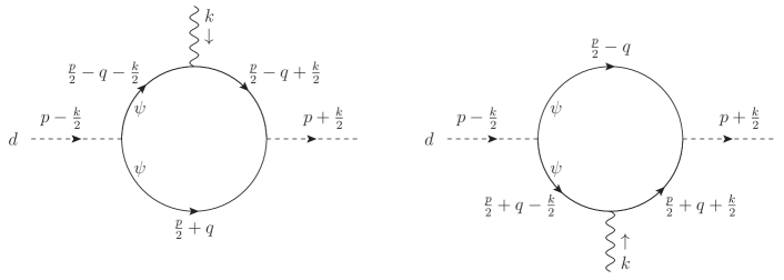
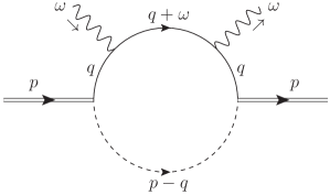
Figure 5: The Feynman diagram for the dipole strength function.
One can check that the dipole strength satisfies the sum rule
(31)
with the charge radius given by Eq. (10). The
energy-weighted sum rule
(32)
is also valid if the logarithmic divergence of the integral on the
left-hand side is regularized by a UV cutoff at the energy of the
Landau pole.
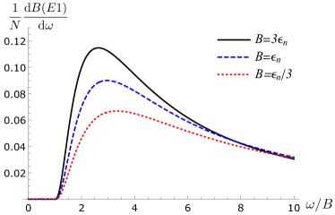
The two sum rules are nontrivial checks of the self-consistency of our
theoretical approach. The predicted shape of the dipole strength
is plotted in Fig. 6 as a function of for
various values of . One sees that the weight of the dipole
strength shifts to larger as decreases.
Figure 6: The dipole strength function, plotted as function of
, for
, , and .
The functions are so normalized by that the area under the theoretical
curve, extended to , is 1.
Applicability to real systems.—The theory described above is
applicable when the binding energy of the halo and the -
two-body virtual energy are smaller than any other energy
scales in the problem. In the real world, MeV
is indeed small. For 6He and 11Li, the two-neutron separation
energy somewhat larger ( and MeV, respectively); in
addition, the existence of near-threshold resonances in the 5He and
10Li subsystem makes the applicability of our theory doubtful.
Nevertheless, let us try to compare our results with existing
experimental data and previous theoretical calculations. For 6He,
Eq. (19) predicts that . In
Ref. [25], it has been argued that the data for 6He
fit the formula , which the authors
derived approximately. Our value is off by about 20%. For 11Li,
we compare our results with those of Ref. [7], where
keV and keV were used. Setting the logarithm
in Eq. (8) to 1,
we find and
, near the center of the error bands
predicted for large energies of the 10Li resonance. The opening
angle (defined as the vertex angle of the isosceles
triangle with sides , , and
) is close to and is again within the
error band. However, for the reasons listed above, it is possible
that the EFT provides only a qualitative guide for 11Li.
The theory presented here may be quantitatively useful for the
22C nucleus if its two-neutron separation energy is indeed as
small as 100 keV [3]. A correction to the EFT
comes from the scattering between the core and one neutron,
parametrized by the irrelevant dimension-6 term
. The contributions from this term to
physical quantities should be suppressed by
relative to the leading-order results, where is the
core-neutron scattering length. Experiment [5]
indicates that fm, so this factor is (0.25 or
0.4 if the upper limit on is taken as 180 or 400 keV,
respectively). Another dimension-6 operator,
,
has its coefficient fixed by the effective range
of the -wave neutron-neutron scattering; its effect is expected to
be similarly suppressed. Other terms, e.g., , have dimension 7 and higher and should be more suppressed.
Corrections from higher-order operators should be computable within
effective field theory.
The presence of the 5He -wave resonance can be taken into account by adding the corresponding field [26].
The present work is expected to open a potential direction to a quantitative study of the halo nuclei in addition to their universal properties.
For the 3He4He2 trimers we expect corrections from
3He–4He scattering to be relatively large: (where is the reduced mass of the
3He–4He system and Å is the
3He–4He scattering length [11]).
Indeed, experiment and quantum Monte Carlo
simulations [27, 28] seem to imply
substantially smaller values for the ratio
compared the one given in Eq. (20).
Acknowledgements.
The authors thank Dario Bressanini, Reinhardt Dörner, Maksim
Kunitski, and especially Hans-Werner Hammer for discussions.
D. T. S. is supported, in part, by the U.S. Department of Energy Grant No. DE-FG02-13ER41958
and a Simons Investigator grant from the Simons Foundation.
M. H. is supported by the U.S. Department of Energy, Office of Science, Office of Nuclear Physics under Grant No. DE-FG0201ER41195 and partially by RIKEN iTHEMS Program (in particular, iTHEMS Non-Equilibrium Working Group and Mathematical Physics Working Group).
References
Zhukov et al. [1993]M. V. Zhukov, B. V. Danilin,
D. V. Fedorov, J. M. Bang, I. J. Thompson, and J. S. Vaagen, Bound state properties of Borromean halo nuclei: 6He
and 11Li, Phys. Rep. 231, 151 (1993).
Tanaka et al. [2010]K. Tanaka, T. Yamaguchi,
T. Suzuki, T. Ohtsubo, M. Fukuda, et al., Observation of a Large Reaction Cross Section in
the Drip-Line Nucleus , Phys. Rev. Lett. 104, 062701 (2010).
Acharya et al. [2013]B. Acharya, C. Ji, and D. R. Phillips, Implications of a matter-radius
measurement for the structure of Carbon-22, Phys. Lett. B 723, 196 (2013), arXiv:1303.6720 .
Togano et al. [2016]Y. Togano et al., Interaction cross section study of the two-neutron halo nucleus
22C, Phys. Lett. B 761, 412 (2016).
Esry et al. [1996]B. D. Esry, C. D. Lin, and C. H. Greene, Adiabatic hyperspherical study of the helium
trimer, Phys. Rev. A 54, 394 (1996).
Note [1]See, e.g., Ref. [28] for a compilation of
theoretical predictions.
Uang and Stwalley [1982]Y. Uang and W. C. Stwalley, The possibility of a
4He2 bound state, effective range theory, and very low energy He–He
scattering, J. Chem. Phys. 76, 5069 (1982).
Note [2]In practice, the running is limited in the UV by the UV
cutoff and in the IR by or , whichever is
larger.
Note [3]In our convention, the dimension of momentum is 1 and energy
is 2.
Note [4]This Lagrangian was, in essence, previously considered in
Ref. [29] for the case of a three-body resonance, i.e., when
the three-body binding energy is negative.
[16]See Supplementary Material for
details.
Note [5]In this scenario, the halo nucleus is bound by the
three-body force. One should note, however, that the effective Lagrangian is
valid irrespective of the nature of the microscopic force responsible for the
binding of the halo nucleus.
Note [6]What we call here the mean-square charge radius should be
understood, for real nuclei, as the difference between the mean-square
point-proton radii of the halo and core nuclei. Similarly, what is later
called the mean-square matter radius is for real nuclei , where and are the mean-square matter radii of the
halo and the core, respectively.
Note [7]In subsequent formulas, is the renormalized coupling in
the on-shell renormalization scheme.
Note [8]This can be done by coupling a gauge field to , where is the baryon charge, is the electric charge, and
and are the atomic and mass numbers, respectively, of the
core.
Note [9]Using the positions of the core and two
neutrons and , we define , , and .
Fedorov et al. [1994]D. V. Fedorov, A. S. Jensen, and K. Riisager, Three-body halos: Gross
properties, Phys. Rev. C 49, 201 (1994).
Peskin and Schroeder [1995]M. E. Peskin and D. V. Schroeder, An Introduction to
Quantum Field Theory (Addison-Wesley, Reading, 1995).
Danilin et al. [2005]B. V. Danilin, S. N. Ershov, and J. S. Vaagen, Charge and matter radii
of Borromean halo nuclei: The 6He nucleus, Phys. Rev. C 71, 057301 (2005).
Son et al. [2021]D. T. Son, M. Stephanov, and H.-U. Yee, Fate of Multiparticle Resonances:
From -Balls to 3He Droplets, (2021), arXiv:2112.03318
.
— Supplementary Material —
Universal Properties of Weakly Coupled Two-Neutron Halo Nuclei
Masaru Hongo and Dam Thanh Son
S1 Field theory: Feynman rules, renormalization
In terms of the bare fields and bare couplings, the Lagrangian of the
theory of the halo nucleus is
(S1)
where is written in Eq. (2). Define the
renormalized halo field and renormalized coupling :
(S2)
the Lagrangian is
(S3)
The Feynman rules are as follows. The dimer propagator is
(S4)
where we introduce the notation
(S5)
The core propagator is
(S6)
and the halo-core-dimer vertex is .
Figure S1: The self-energy of the halo nucleus. The dash line in the
loop is the dimer propagator, while the solid line is the propagator
of the core.
The self-energy of the field is given by a one-loop diagram,
(Fig. S1)
(S7)
Closing the contour in the lower half-plane,
we find
(S8)
Performing a shift , we then get
(S9)
where
(S10)
is the reduced mass of the core-dimer system.
The full inverse propagator of the halo is then
(S11)
The integral over is quadratically divergent in the UV. We
assume it is regularized by e.g., a momentum cutoff or by dimensional
regularization. We use the on-shell renormalization scheme, where
the following two conditions are imposed:
where we have used Eq. (S15). This is just the
statement that the total charge is equal to 1
in our normalization.
Expanding Eq. (S21) to second order in , we
then find the charge radius from
:
(S24)
which can be written as
(S25)
where
(S26)
Integrating by part, this can be reduced into the form
(S27)
Evaluating the integral, one obtains
Eq. (11). The result for the charge radius also coincides
with the value obtained from a sum rule for the dipole strength
function, computed in Section S4.
S3 Neutron radius
S3.1 Effective coupling of the dimer to the “neutron-number photon”
The two diagrams contributing to the effective coupling of the dimer
to the “neutron-number photon” are depicted in
Fig. S3. They sum up to
(S28)
Performing the integral over , this becomes
(S29)
Expanding to quadratic order in and ,
one can write the result in terms of the three Galilean invariant quantities
(S30)
as
(S31)
where
(S32)
(S33)
(S34)
Figure S3: The diagrams contributing to the effective coupling of a “neutron-number photon” to the dimer field.
S3.2 Calculation of the neutron radius
We imagine that there exists a gauge boson that couples to the
neutrons outside the core, but not to the core. The “neutron form
factor” receives a contribution from the Feynman diagram in
Fig. S4, and defined by
Figure S4: The Feynman diagram that contributes to the neutron
form factor of the halo nucleus.
Here is the effective vertex of the coupling of
the dimer to the “neutron-number photon.” This vertex has been
evaluated in Sec. S3.1 to second order in the photon
momentum to
(S37)
where , .
Integrating over the , closing the contour in the lower
half-plane, one picks up the pole from the core propagator
(S38)
At the kinematic point (S19), the neutron form
factor of the halo nucleus is, to quadratic order in ,
To find the dipole strength function, one needs to evaluate the
Feynman diagrams, one of which is drawn on
Fig. S5
(S43)
where . Closing the contour in the lower
half-plane, the imaginary part comes from the pole in .
(S44)
Evaluating the integral one finds
(S45)
with the function defined in Eq. (30).
From this one obtains Eq. (29).
Figure S5: The Feynman diagram determining the dipole strength
function. A second diagram obtained by reversing the direction of
momentum flow on the two photon lines contributes to but
not to its imaginary part when .
S5 Relationships between various mean square radii
Let denote the position of the core, and and
those of the two neutrons.
Assume that the center of mass is at the origin,
(S46)
then the coordinates of every particle can be express through
and :
(S47)
(S48)
Now notice that due to the symmetry of the ground-state wavefunction of the halo with respect to exchanging and , one can derive relationships between different
mean-square radii.
For example
(S49)
Analogously
(S50)
(S51)
where we used Eq. (S46) to derive the second relation.