A novel way of measuring the gas disk mass of protoplanetary disks using $\mathrm{N}_{2}\mathrm{H}^{+}$ and $\mathrm{C}^{18}\mathrm{O}$

Abstract

Measuring the gas mass of protoplanetary disks, the reservoir available for giant planet formation, has proven to be difficult. We currently lack a far-infrared observatory capable of observing HD, and the most common gas mass tracer, CO, suffers from a poorly constrained CO-to-H₂ ratio. Expanding on previous work, we investigate if $\mathrm{N}_{2}\mathrm{H}^{+}$, a chemical tracer of CO poor gas, can be used to observationally measure the CO-to-H₂ ratio and correct CO-based gas masses. Using disk structures obtained from the literature, we set up thermochemical models for three disks, TW Hya, DM Tau and GM Aur, to examine how well the CO-to-H₂ ratio and gas mass can be measured from $\mathrm{N}_{2}\mathrm{H}^{+}$ and $\mathrm{C}^{18}\mathrm{O}$ line fluxes. Furthermore, we compare these gas masses to independently gas masses measured from archival HD observations. The $\mathrm{N}_{2}\mathrm{H}^{+}$ (3-2)/$\mathrm{C}^{18}\mathrm{O}$ (2-1) line ratio scales with the disk CO-to-H₂ ratio. Using these two lines, we measure $4.6\times 10^{-3}\ \mathrm{M}_{\odot}\leq M_{\rm disk}\leq 1.1\times 10^{-1}\ \mathrm{M}_{\odot}$ for TW Hya, $1.5\times 10^{-2}\ \mathrm{M}_{\odot}\leq M_{\rm disk}\leq 9.6\times 10^{-2}\ \mathrm{M}_{\odot}$ for GM Aur and $3.1\times 10^{-2}\ \mathrm{M}_{\odot}\leq M_{\rm disk}\leq 9.6\times 10^{-2}\mathrm{M}_{\odot}$ for DM Tau. These gas masses agree with values obtained from HD within their respective uncertainties. The uncertainty on the $\mathrm{N}_{2}\mathrm{H}^{+}$ + $\mathrm{C}^{18}\mathrm{O}$ gas mass can be reduced by observationally constraining the cosmic ray ionization rate in disks. These results demonstrate the potential of using the combination of $\mathrm{N}_{2}\mathrm{H}^{+}$ and $\mathrm{C}^{18}\mathrm{O}$ to measure gas masses of protoplanetary disks.

1 Introduction

The gas mass of protoplanetary disks is a crucial ingredient for planet formation theories (e.g. Mordasini 2018). On a macro scale, the gas mass represents the total mass budget available for forming gas giants. Combined with the stellar accretion rate and mass loss rate it determines the lifetime of the disk and therefore sets the timescale for giant planet formation. On a micro scale, the gas density and gas-to-dust ratio regulate the dynamics of dust grains and larger bodies in the disk. The rate at which the dust grows, settles towards the midplane and drift inward toward the central star all depend on how much gas is present in the disk (see, e.g., Birnstiel et al. 2012).

Measuring the gas mass of disks from observations has proven difficult. The gas is predominantly made up of molecular hydrogen ($\mathrm{H}_{2}$), a light, symmetric molecule without a permanent dipole moment that does not significantly emit at temperatures typically found in protoplanetary disks. Hydrogen deuteride (HD) has been shown to be a promising indirect tracer of the gas mass. HD is chemically similar to $\mathrm{H}_{2}$ and thus closely follows the distribution of $\mathrm{H}_{2}$ (see Trapman et al. 2017). Contrary to $\mathrm{H}_{2}$, HD has a small dipole moment and can emit from a significant part of the disk. Using Hershel, the HD $J=1-0$ line has been detected in three protoplanetary disks: TW Hya, GM Aur and DM Tau (Bergin et al., 2013; McClure et al., 2016), allowing us to accurately measure their gas masses. HD 1-0 upper limits have also been used to put constraints on the gas masses of Herbig disks (Kama et al., 2020). With the end of the Herschel mission, we currently lack a far-infrared observatory capable of observing HD in disks.

Instead, the most often used gas mass tracer is carbon monoxide (CO), the second most abundant molecule in the gas of protoplanetary disks. CO emission is bright at millimeter wavelengths and has been detected in almost all protoplanetary disks. The emission of its main isotopologue, ${}^{12}\mathrm{CO}$, is optically thick in disks, but its less abundant isotopologues, e.g. ${}^{13}\mathrm{CO}$ and $\mathrm{C}^{18}\mathrm{O}$, are most often optically thin. Emission from rarer isotopologues like ¹³C¹⁸O or ¹³C¹⁷O is even more optically thin, but these weak lines are less suitable for large gas mass surveys (see e.g. Zhang et al. 2017; Booth et al. 2019). The main uncertainty when using CO as gas mass tracer is the CO-to-$\mathrm{H}_{2}$ abundance ratio ($x_{\rm CO}$). CO is a chemically stable molecule that in the warm gas of protoplanetary disks is expected to have a relatively constant abundance of $x_{\rm CO}\approx 10^{-4}$. Two main processes reduce $x_{\rm CO}$ in the disk. In the irradiated surface layer of the disk far-ultraviolet photons will photo-dissociated CO until it can build up a sufficient column to shield itself against this process. Close to the cold midplane of the disk CO freezes out onto the surface of dust grains. Both of these processes have been extensively studied and are well understood (see, e.g. van Dishoeck & Black 1988; van Zadelhoff et al. 2001; Visser et al. 2009; Miotello et al. 2014). By incorporating them in physical-chemical disk models these processes can be accounted for, allowing us to measure disk masses from ${}^{13}\mathrm{CO}$ and $\mathrm{C}^{18}\mathrm{O}$ line fluxes (e.g. Williams & Best 2014; Miotello et al. 2016).

However, there is increasing observational evidence that we are overlooking one or more processes that reduce $x_{\rm CO}$ in protoplanetary disks. When compared to gas masses derived independently from HD, the CO-based gas masses are found to be $5\,-\,100\,\times$ lower, even after including the effects of photo-dissociation and freeze-out (see, e.g. Favre et al. 2013; Schwarz et al. 2016; Kama et al. 2016; McClure et al. 2016; Trapman et al. 2017; Calahan et al. 2021). This could imply that the low CO-based gas masses found in disk surveys carried out with the Atacama Large Millimiter/submillimeter Array (ALMA) are severely underestimating the gas masses of protoplanetary disks (see, e.g. Ansdell et al. 2016; Miotello et al. 2017; Long et al. 2017). Several processes have been suggested to cause this low $x_{\rm CO}$, such as the chemical conversion of CO into more complex species (e.g. Aikawa et al. 1997; Furuya & Aikawa 2014; Yu et al. 2016, 2017; Bosman et al. 2018; Schwarz et al. 2018). Alternatively, grain growth can lock up CO into larger dust bodies that settle towards the midplane (e.g. Bergin et al. 2010, 2016; Kama et al. 2016; Krijt et al. 2018, 2020). Irrespective of what causes the low CO abundance, we need to measure $x_{\rm CO}$ in order to reliably measure disk gas masses using CO.

In this Letter we examine $\mathrm{N}_{2}\mathrm{H}^{+}$, a chemical tracer of CO-poor gas, as a potential calibrator of the CO abundance in protoplanetary disks. $\mathrm{N}_{2}\mathrm{H}^{+}$ is formed through proton transfer from H${}_{3}^{+}$ to N₂. If CO is present in the gas phase it competes with N₂ for the available H${}_{3}^{+}$, thus impeding the formation of $\mathrm{N}_{2}\mathrm{H}^{+}$. In addition, $\mathrm{N}_{2}\mathrm{H}^{+}$ is rapidly destroyed by gas-phase CO. As a result, $\mathrm{N}_{2}\mathrm{H}^{+}$ is therefore only abundant if there is a lack of gas-phase CO. These properties have seen $\mathrm{N}_{2}\mathrm{H}^{+}$ be successfully used to locate the CO iceline (e.g. Qi et al. 2013, 2015, 2019; Huang & Öberg 2015; van ’t Hoff et al. 2017).

For the disk as a whole, this chemical relation between $\mathrm{N}_{2}\mathrm{H}^{+}$ and CO means higher $\mathrm{N}_{2}\mathrm{H}^{+}$ abundances, and hence higher fluxes, when CO is underabundant (see Figure 1). The anti-correlation between the $\mathrm{N}_{2}\mathrm{H}^{+}$ flux and the CO abundance was previously studied in Anderson et al. (2019), who showed that a CO abundance $x_{\rm CO}\leq 10^{-6}$ is required to explain the $\mathrm{N}_{2}\mathrm{H}^{+}$ and CO line fluxes of two disks in Upper Sco. Here we expand upon their work and examine if $\mathrm{N}_{2}\mathrm{H}^{+}$ can be used to observationally measure the global CO abundance in protoplanetary disks and therefore, the gas mass. To test this hypothesis we select the three disks with HD $J=1-0$ detections, TW Hya, DM Tau and GM Aur, for which we have independent measurements of the disk gas mass and global CO abundance.

The structure of this Letter is as follows: in Section 2 we set up thermochemical disk models based on disk structures obtained from the literature and use the $\mathrm{C}^{18}\mathrm{O}$ $J=2-1$ integrated flux to select the combinations of CO abundance and disk gas mass that reproduce the $\mathrm{C}^{18}\mathrm{O}$ observations. Combining a simple $\mathrm{N}_{2}\mathrm{H}^{+}$ chemical network with our thermochemical models to calculate $\mathrm{N}_{2}\mathrm{H}^{+}$ abundances and excitation, we show in Section 3 that the $\mathrm{N}_{2}\mathrm{H}^{+}$ $J=3-2$ integrated line flux, combined with the $\mathrm{C}^{18}\mathrm{O}$ 2-1 flux, constrains the average CO abundance in the disk. For a reasonable range of cosmic ray ionization rates we show that correcting the CO-based gas mass using $x_{\rm CO}$ derived from $\mathrm{N}_{2}\mathrm{H}^{+}$ and $\mathrm{C}^{18}\mathrm{O}$ agrees with the gas disk mass measured from HD. In Section 4 we examine the cosmic ray ionization rates in our three disks and we discuss some of the caveats of this study. We summarize our findings in Section 5.

Table 1: Source information

Source	$M_{\star}$	$L_{\star}$	Teff	$L_{\rm UV}$	$L_{X}$	dist	$M_{\rm gas}$ (HD)	$M_{\rm gas}$ (CO)	$\mathrm{N}_{2}\mathrm{H}^{+}$ $3-2$	$\mathrm{C}^{18}\mathrm{O}$ $2-1$	HD $1-0$
	(M⊙)	(L⊙)	(K)	(erg s-1)	(erg s-1)	(pc)	(M⊙)	(M⊙)	(Jy km/s)	(Jy km/s)	(W m-2)
				$\times 10^{30}$	$\times 10^{30}$		$\times 10^{-2}$	$\times 10^{-2}$			$\times 10^{-18}$
TW Hya	0.8	0.28	4110	$27$	$1.6$	59	0.77-2.5	0.05-0.5	$2.0\pm 0.21$	$0.57\pm 0.06$	$6.3\pm 0.7$
DM Tau	0.53	0.24	3705	$3.0$	$0.3$	145	1-4.7	0.1-1	$1.286\pm 0.17$	$1.11\pm 0.11$	$1.6\pm 0.4$
GM Aur	1.1	1.2	4350	$28$	$1.4$	159	20	0.8	$1.487\pm 0.18$	$1.024\pm 0.097$	$2.5\pm 0.5$
Refs	(1,2,3)			(4,5,6)	(7,6)	(3)	(8,9,10,11)	(12,13,14,15)	(16,17)	(9,18,19)	(20,10)

Notes: for details on the adopted disk structures, see Kama et al. (2016) for TW Hya, Zhang et al. (2019) for DM Tau and Zhang et al. (2021) for GM Aur. ALMA line fluxes include a 10% systematic flux uncertainty.

References: (1) Andrews et al. (2011), (2) Kenyon & Hartmann (1987), (3) Gaia Collaboration et al. (2018), (4) Cleeves et al. (2015), (5) Dionatos et al. (2019) (6) Brickhouse et al. (2010), (7) Henning et al. (2010) (8) Trapman et al. (2017), (9) Calahan et al. (2021), (10) McClure et al. (2016), (11) Schwarz et al. (2021), (12) Thi et al. (2010), (13) Miotello et al. (2016), (14) Zhang et al. (2019), (15) Zhang et al. (2021), (16) Qi et al., in prep., (17) Qi et al. (2019), (18) Bergner et al. (2019), (19) Oberg et al. (2021), (20) Bergin et al. (2013)

2 Model setup

For running our models we use the thermochemical code Dust and Lines (DALI; Bruderer et al. 2012; Bruderer 2013). For a physical 2D disk structure and stellar spectrum DALI calculates the thermal and chemical structure of the disk self-consistently. The computation is split into three steps: first, the radiative transfer equation is solved using a 2D Monte Carlo method to calculate the dust temperature structure and the internal radiation field. Next, the abundances of molecular and atomic species are calculated at each point in the disk by solving the time-dependent chemistry. We include CO and HD isotope-selective photodissociation and chemistry following Miotello et al. (2014) and Trapman et al. (2017). The excitation levels of all species are computed using a non-LTE calculation. From the excitation levels the gas temperature is calculated by balancing heating and cooling processes. As both the chemistry and excitation depend on the gas temperature, an iterative calculation is used to find a self-consistent solution. Finally, the model is ray-traced to produce integrated line fluxes and line profiles. For a more detailed description of the code, see Appendix A of Bruderer et al. (2012).

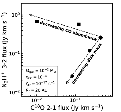
Figure 1: Concept of how $\mathrm{N}_{2}\mathrm{H}^{+}$ and $\mathrm{C}^{18}\mathrm{O}$ enable us to distinguish between disks with low disk masses and low CO abundance. Starting from the fiducial model (diamond) on the right, points show the change in $\mathrm{N}_{2}\mathrm{H}^{+}$ 3-2 and $\mathrm{C}^{18}\mathrm{O}$ 2-1 line flux when either the disk mass (circles) or CO abundance (squares) is decreased, with decrements of factors of ten. Relevant disk parameters of the fiducial model are shown in the bottom left.

For the three disks with HD $J=1-0$ detections, we obtain disk structures from the literature (TW Hya: Kama et al. 2016; DM Tau: Zhang et al. 2019; GM Aur: Zhang et al. 2021). For each of these models, the disk structure was fitted using a combination of the spectral energy density (SED) and resolved millimeter continuum and line emission. With these fiducial models our approach is as follows: we set up and run a set of models with different combinations of $M_{\rm gas}$ and $x_{\rm CO}$. From this set of models we find the subset that reproduces the integrated $\mathrm{C}^{18}\mathrm{O}\ J=2-1$ flux. Specifically we select those models that satisfy $F_{\mathrm{C}^{18}\mathrm{O}}^{\rm model}-F_{\mathrm{C}^{18}\mathrm{O}}^{\rm obs}\leq 3\sigma_{\mathrm{C}^{18}\mathrm{O}}^{\rm obs}$. Our models show that the $\mathrm{C}^{18}\mathrm{O}\ J=2-1$ flux is mostly optically thin, only becoming optically thick in the inner disk $(R<0.5-1\times R_{c})$. Note that this inner disk area encompasses $40-60\%$ of the total gas mass in each disk. These models represent the combinations of gas disk mass and CO abundance that could explain the $\mathrm{C}^{18}\mathrm{O}$ observations. Models where $x_{\rm CO}<10^{-4}$ represent scenarios where some amount of the gas-phase CO is either chemically converted or locked up as ice on large dust grains. By lowering the CO abundance in this way we remain agnostic on how the CO is removed from the gas and focus on the end result, an underabundance of gaseous CO in disks. The model selection is visualized in Figure 2.

For the models that reproduce the observed $\mathrm{C}^{18}\mathrm{O}$ flux, we calculate the $\mathrm{N}_{2}\mathrm{H}^{+}$ chemistry using the chemical network presented in van ’t Hoff et al. (2017). Briefly, this network includes the production of H${}_{3}^{+}$ through cosmic-ray induced ionization of H₂, freeze-out and desorption of CO and N₂, formation of $\mathrm{N}_{2}\mathrm{H}^{+}$ and HCO⁺ through reactions of H${}_{3}^{+}$ with N₂ and CO, respectively, and the destruction of $\mathrm{N}_{2}\mathrm{H}^{+}$ through reacting with CO (see their Figure 2). Using this simple network instead of the larger network in DALI has the advantage of being easier to understand what factors could affect the $\mathrm{N}_{2}\mathrm{H}^{+}$ abundance and fluxes (see also Section 4.1).

Our approach is the following: we take the gas temperature structure and CO and N₂ abundance calculated with DALI and use these to compute the $\mathrm{N}_{2}\mathrm{H}^{+}$ abundance structure using the chemical $\mathrm{N}_{2}\mathrm{H}^{+}$ network. The main free parameter in this network is the cosmic ray ionization rate $\zeta_{\rm CR}$. We note that $\zeta_{\rm CR}$ is the only source of ionization in our network. While cosmic rays are likely the dominant ionization source in the region of the disk where $\mathrm{N}_{2}\mathrm{H}^{+}$ is abundant (e.g. Aikawa et al. 2015, 2021), the values of $\zeta_{\rm CR}$ in this work should be read as upper limits, as other ionization processes such as X-rays and the decay of radionuclids could still contribute (see e.g. Seifert et al. 2021). We compute the $\mathrm{N}_{2}\mathrm{H}^{+}$ abundance structure for $\zeta_{\rm CR}=10^{-19},10^{-18}\ \mathrm{and}\ {10^{-17}\ \mathrm{s}^{-1}}$. The $\mathrm{N}_{2}\mathrm{H}^{+}$ abundance structure is then re-inserted into the DALI model to calculate the excitation and synthetic line emission.

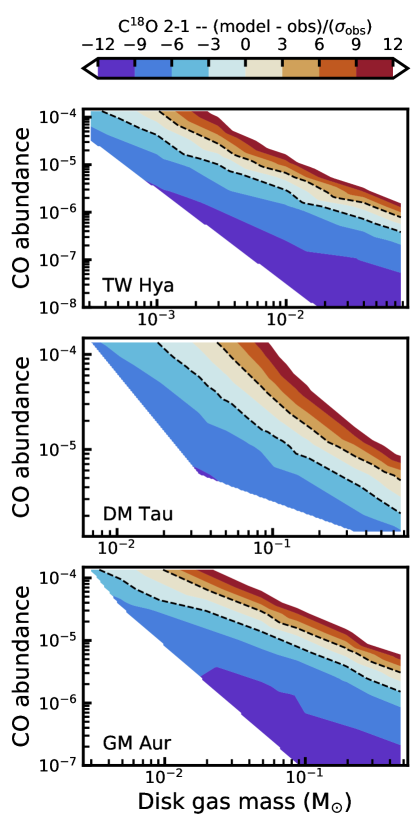
Figure 2: Comparison between the observed $\mathrm{C}^{18}\mathrm{O}$ $J=2-1$ integrated line flux and our models with different combinations of disk gas mass and CO abundance. Colors show how close the model $\mathrm{C}^{18}\mathrm{O}$ line flux is to the observations, expressed in terms of the uncertainty on the $\mathrm{C}^{18}\mathrm{O}$ line flux. $(\sigma_{\rm obs})$. Dashed black lines highlight the part of the $M_{\rm gas}$-$x_{\rm CO}$ parameters space where model $\mathrm{C}^{18}\mathrm{O}$ fluxes are within $3\sigma_{\rm obs}$. Darker shades of blue (red) marks parameter space where the model underproduces (overproduces) the observed flux.

3 Results

Figure 3 shows the $\mathrm{N}_{2}\mathrm{H}^{+}$ (3-2)/$\mathrm{C}^{18}\mathrm{O}$ (2-1) integrated flux ratio versus the CO abundance for the three disks. Note that each of the models reproduces the $\mathrm{C}^{18}\mathrm{O}$ integrated flux within $3\sigma$. The flux ratio clearly increases as the CO abundance decreases. This trend is similar to the one found by Anderson et al. (2019) (see their Figures 5 and 9). For GM Aur the trend flattens at the highest disk masses where both lines start to become optically thick. The figure also shows that lowering $\zeta_{\rm CR}$ reduces the flux ratio. A lower $\zeta_{\rm CR}$ equals less ionization and therefore less $\mathrm{N}_{2}\mathrm{H}^{+}$ and a lower $\mathrm{N}_{2}\mathrm{H}^{+}$ 3-2 flux. The $\mathrm{C}^{18}\mathrm{O}$ flux is not affected, but we should note that our chemical network does not include the chemical conversion of CO into more complex species, where $\zeta_{\rm CR}$ plays a large role (see Schwarz et al. (2018, 2019); Bosman et al. (2018)). By comparing our models to the observations shown in gray, we can derive the global CO abundance of the disk.

Both TW Hya and GM Aur require a CO abundance $\leq 10^{-4}$ to match the $\mathrm{N}_{2}\mathrm{H}^{+}$/$\mathrm{C}^{18}\mathrm{O}$ line ratio. Specifically, TW Hya requires $x_{\rm CO}\leq 1.3\times 10^{-5}$ and GM Aur requires $x_{\rm CO}\leq 6.5\times 10^{-5}$. For DM Tau the CO abundance does not have to be lowered to match the line ratio. Rather the models show that a lower cosmic ionization rate $\sim\,5\times 10^{-18}\ \mathrm{s}^{-1}$ is needed to reproduce the line ratio with a CO abundance of $10^{-4}$. The lower bound on the CO abundance depends on the cosmic ionization rate. If we assume a lower bound of $\zeta_{\rm CR}=10^{-19}\ \mathrm{s}^{-1}$ in disks (see, e.g. Cleeves et al. 2015), we can constrain the CO abundances to $3.5\times 10^{-7}\leq x_{\rm CO}\leq 1.3\times 10^{-5}$ for TW Hya, $1.1\times 10^{-5}\leq x_{\rm CO}\leq 6.5\times 10^{-5}$ for GM Aur and $2.3\times 10^{-5}\leq x_{\rm CO}\leq 1.3\times 10^{-4}$ for DM Tau. As shown here, a two order of magnitude uncertainty in $\zeta_{\rm CR}$ results in a factor of $5-37$ uncertainty in the CO abundance and thus the gas disk mass. Constraining the cosmic-ray ionization rate in disks using observations of, for example, H¹³CO⁺ and N₂D⁺ will reduce the uncertainty on the gas disk mass (see, e.g., Cleeves et al. 2015; Aikawa et al. 2021).

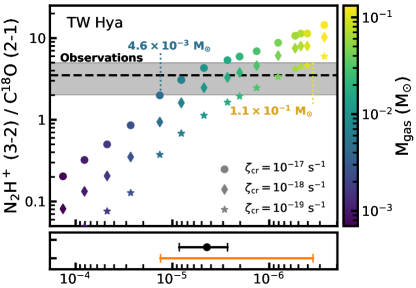
Figure 3: $\mathrm{N}_{2}\mathrm{H}^{+}$ (3-2)/$\mathrm{C}^{18}\mathrm{O}$ (2-1) flux ratio versus the CO abundance. Points denote individual models, where the shape shows the assumed cosmic ray ionization rate $(\zeta_{\rm CR})$. The colors show the gas mass of the disk. The observed $\mathrm{N}_{2}\mathrm{H}^{+}$ (3-2)/$\mathrm{C}^{18}\mathrm{O}$ (2-1) ratio is shown as a black dashed line, with the gray shaded region showing the $3\sigma$ uncertainty. For reference we included the lowest and highest disk mass that reproduce these observations, assuming $10^{-19}\ \mathrm{s}^{-1}\leq\zeta_{\rm CR}\leq 10^{-17}\ \mathrm{s}^{-1}$. The smaller panels under each main panel show the CO abundance ranges that reproduce the observations. Here the orange bar corresponds to $\mathrm{N}_{2}\mathrm{H}^{+}$ (3-2) and $\mathrm{C}^{18}\mathrm{O}$ (2-1), with $10^{-19}\ \mathrm{s}^{-1}\leq\zeta_{\rm CR}\leq 10^{-17}\ \mathrm{s}^{-1}$. The black bar instead shows the CO abundance constrained by HD 1-0 and $\mathrm{C}^{18}\mathrm{O}$ (2-1).

Using these CO abundances we can now correct the CO-based gas mass for the underabundance of CO and obtain the true gas disk mass. This yields $4.6\times 10^{-3}\ \mathrm{M}_{\odot}\leq M_{\rm disk}\leq 1.1\times 10^{-1}\ \mathrm{M}_{\odot}$ for TW Hya, $1.5\times 10^{-2}\ \mathrm{M}_{\odot}\leq M_{\rm disk}\leq 9.6\times 10^{-2}\ \mathrm{M}_{\odot}$ for GM Aur and $3.1\times 10^{-2}\ \mathrm{M}_{\odot}\leq M_{\rm disk}\leq 9.6\times 10^{-2}\mathrm{M}_{\odot}$ for DM Tau. By including $\mathrm{N}_{2}\mathrm{H}^{+}$ we have increased the accuracy of the measured gas disk mass by a factor 5-10 compared to CO-based gas masses, by correcting for the fact that CO is underabundant in the gas by a factor of 5-10 in our disks. As mentioned above, the precision of the gas mass measurement can be improved by constraining the cosmic ray ionization rate. Thus, combining $\mathrm{N}_{2}\mathrm{H}^{+}$ and $\mathrm{C}^{18}\mathrm{O}$ allows us to break the degeneracy between gas disk mass and CO abundance shown in Figure 2 and gives us a recipe for measuring gas disk masses.

It is interesting to compare our new gas disk masses to those measured independently from HD 1-0 integrated line fluxes. To be consistent with the disk structures assumed in the rest of this work, we opt to use our models to measure $M_{\rm gas}^{HD}$ rather than using literature values (see Table 1). Figure 5 in Appendix A shows how $M_{\rm gas}^{HD}$ is derived from the HD 1-0 integrated flux. Uncertainties on the masses are derived by propagating the $3\sigma$ uncertainties of the line flux. The HD-based based disk masses for TW Hya and GM Aur are consistent with literature values (see Table 1). Only for DM Tau do we find a substantially higher disk mass than previously found, due to our model being more extended, and thus having lower average gas temperature, than the model in McClure et al. (2016). As HD predominantly emits from warm gas, it should be noted that the accuracy of HD as a gas mass tracer depends on how well the temperature structure of the disk is known (see e.g. Trapman et al. 2017; Calahan et al. 2021). If the disks are significantly warmer than our models we would overestimate their gas mass. This is unlikely to be a large effect however as the disk structures used here reproduce several optically thick CO lines which trace the gas temperature.

The disk mass obtained for DM Tau warrants some further discussion. Based on the HD 1-0 flux and uncertainty, we find a maximum disk mass of $M_{\rm gas}=0.55\ \mathrm{M}_{\odot}$, which would make the disk approximately as massive as the star. Such a high disk mass is unphysical, as disk would become gravitationally unstable before it could reach this disk mass. To find a more physical maximum disk mass, we calculate the Toomre Q parameter Toomre (1964) using the surface density and midplane temperature profiles from our models. For a gas disk mass $M_{\rm gas}\approx 0.2\ \mathrm{M}_{\odot}$ we find $Q\lesssim 1.7$, which is the approximate threshold where instabilities can start to develop in numerical simulations of disks (e.g. Helled et al. 2014). For the rest of this work we will use $M_{\rm gas}=0.2\ \mathrm{M}_{\odot}$ as a more realistic maximum disk mass for DM Tau.

Figure 4 compares the gas mass obtained from combining $\mathrm{N}_{2}\mathrm{H}^{+}$ and $\mathrm{C}^{18}\mathrm{O}$ to the gas mass measured from HD 1-0 (see Figure 5). Lining up the two mass ranges of each of the three sources, we find good agreement. For DM Tau and GM Aur the $\mathrm{N}_{2}\mathrm{H}^{+}$ + $\mathrm{C}^{18}\mathrm{O}$ gas masses are overall slightly lower compared to the HD gas mass. The lower end of the $\mathrm{N}_{2}\mathrm{H}^{+}$ + $\mathrm{C}^{18}\mathrm{O}$ gas mass range corresponds to the highest assumed $\zeta_{\rm CR}$, suggesting that these disks have a lower cosmic ray ionization rate (see Section 4.1 for a further discussion on this topic). The uncertainty on the $\mathrm{N}_{2}\mathrm{H}^{+}$ + $\mathrm{C}^{18}\mathrm{O}$ gas mass for DM Tau and GM Aur is similar to the uncertainty of the HD-based gas mass measured from their low signal-to-noise HD 1-0 detections. For TW Hya, where HD was detected with comparatively high signal-to-noise, the resulting $M_{\rm gas}^{HD}$ range is more narrow and matches the gas mass derived from $\mathrm{N}_{2}\mathrm{H}^{+}$ and $\mathrm{C}^{18}\mathrm{O}$ if a high cosmic ray ionization rate is used.

While based on only a small sample of disks, Figure 4 shows that combination of $\mathrm{N}_{2}\mathrm{H}^{+}$ and $\mathrm{C}^{18}\mathrm{O}$ integrated line fluxes is a promising new recipe for measuring gas masses of protoplanetary disks

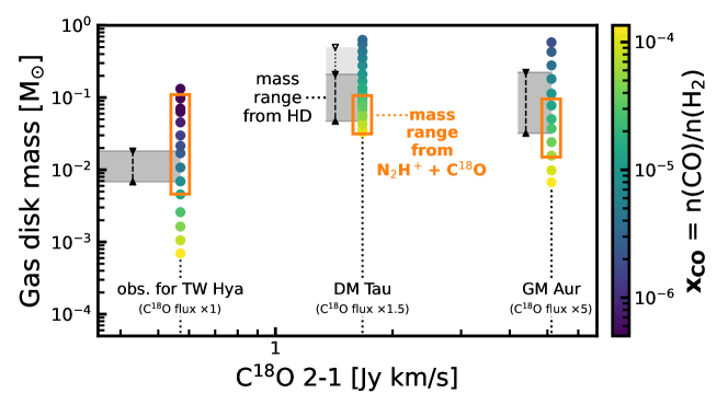
Figure 4: Comparison of the mass ranges obtained from HD 1-0 (gray shaded region) and the combination of $\mathrm{N}_{2}\mathrm{H}^{+}$ and $\mathrm{C}^{18}\mathrm{O}$ (orange box). Note that for $\mathrm{N}_{2}\mathrm{H}^{+}$ and $\mathrm{C}^{18}\mathrm{O}$ we have assumed $10^{-19}\ \mathrm{s}^{-1}\leq\zeta_{\rm CR}\leq 10^{-17}\ \mathrm{s}^{-1}$. Points show individual models, with their color showing the CO abundance. For DM Tau, the transition from dark to light gray shows where $M_{\rm disk}=0.2\ \mathrm{M}_{\odot}$. For a higher disk mass there should be signs of gravitational instability in the disk, which have not been seen in observations (see Section 3 for more details).

4 Discussion

4.1 Constraining the cosmic ray ionization rate

As previously discussed, the gas disk mass derived from $\mathrm{N}_{2}\mathrm{H}^{+}$ and $\mathrm{C}^{18}\mathrm{O}$ depends on the assumed $\zeta_{\rm CR}$. In our comparison between different gas disk mass estimates we have taken the dependence on $\zeta_{\rm CR}$ as an addition uncertainty on the CO abundance estimated from $\mathrm{N}_{2}\mathrm{H}^{+}$. However, we can also examine the overlap between the gas disk mass from HD and one from $\mathrm{N}_{2}\mathrm{H}^{+}$ and $\mathrm{C}^{18}\mathrm{O}$ to put constraints on $\zeta_{\rm CR}$. Taking the gas disk mass derived from the HD observations, we determine the range of $\zeta_{\rm CR}$ for which our models are able to reproduce the $\mathrm{N}_{2}\mathrm{H}^{+}$ 3-2 integrated flux.

We find a clear dichotomy in cosmic ray ionization rates. One disk, TW Hya, is most consistent with a relatively high cosmic ray ionization rate, $5\times 10^{-18}\leq\zeta_{\rm CR}\leq 1\times 10^{-17}\ \mathrm{s}^{-1}$, while the other two disks are more consistent with low rates, $\zeta_{\rm CR}\leq 1\times 10^{-18}\ \mathrm{s}^{-1}$ for DM Tau and $\zeta_{\rm CR}\leq 5\times 10^{-19}\ \mathrm{s}^{-1}$ for GM Aur, respectively. The low $\zeta_{\rm CR}$ for DM Tau and GM Aur are consistent with earlier findings (see, e.g. Cleeves et al. 2015). In particular, Aikawa et al. (2021) found a low cosmic ray ionization $(\leq 10^{-18}\ \mathrm{s}^{-1})$ for GM Aur based on deep observations of $\mathrm{N}_{2}\mathrm{H}^{+}$ and N₂D⁺. Finding a high $\zeta_{\rm CR}$ for TW Hya is more puzzling. In an earlier study, Cleeves et al. (2015) modeled $\mathrm{N}_{2}\mathrm{H}^{+}$, HCO⁺ and H¹³CO⁺, in combination with CO isotopologues and HD, observations of TW Hya, finding that the observations are best reproduced by a moderately hard X-ray spectrum and a low cosmic ray ionization rate $(\zeta_{\rm CR}\leq 10^{-19}\mathrm{s}^{-1})$. In their models, a high $\zeta_{\rm CR}$ such as the one found in this work results in a peak of the $\mathrm{N}_{2}\mathrm{H}^{+}$ 4-3 emission at $\sim\,130$ au, much further out than the observed location at $\sim\,45$ au (see Qi et al. 2013). Interestingly, the peak of $\mathrm{N}_{2}\mathrm{H}^{+}$ 4-3 radial intensity profile in our TW Hya model with $\zeta_{\rm CR}=10^{-17}\ \mathrm{s}^{-1}$ lies further inward and matches the observed peak location (cf. van ’t Hoff et al. 2017).

There are three key differences between the models in Cleeves et al. (2015) and the models presented in this work. The first is the assumed surface density structure. Our TW Hya models have a characteristic radius of $R_{c}=35$ au, whereas the models in Cleeves et al. (2015) use $R_{c}=150$ au and truncate the disk at $200$ au. However, Cleeves et al. (2015) showed that this difference in surface density has minimal impact on the $\mathrm{N}_{2}\mathrm{H}^{+}$ column densities (see their appendix C). A similar test where we change the surface density in our models confirms that this cannot explain the difference in $\mathrm{N}_{2}\mathrm{H}^{+}$ 4-3 intensity profiles. The second is the chemical network. In this work we use a simplified $\mathrm{N}_{2}\mathrm{H}^{+}$ chemical network that only includes its dominant formation and destruction pathways. This suggests that there are one or more reactions in network used in Cleeves et al. 2015 that significantly affect the $\mathrm{N}_{2}\mathrm{H}^{+}$ chemistry that are not included in our network. One such reaction could be the non-thermal desorption of N₂ and CO. However, van ’t Hoff et al. 2017 showed that an increased desorption rate has a negligible effect on the $\mathrm{N}_{2}\mathrm{H}^{+}$ 4-3 emission profile (see their Appendix D). Finally, we only include ionization through cosmic rays, which is the dominant source for ionization close to the disk midplane. Cleeves et al. (2015) also include X-ray ionization, which could affect $\mathrm{N}_{2}\mathrm{H}^{+}$ abundance higher up in the disk. Reconciling the two models requires a full comparison between the two approaches, which is beyond the scope of this paper. We do note that the Cleeves et al. (2015) model with $\zeta_{\rm CR}\approx 10^{-18}\ \mathrm{s}^{-1}$ combined with a softer X-ray spectrum also reproduces the observed $\mathrm{N}_{2}\mathrm{H}^{+}$ 4-3 emission, which is more similar to the value found in this work.

4.2 Caveats

Here we briefly discuss some of the caveats and uncertainties that could effect our results. A detailed investigation of these caveats is beyond the scope of this Letter and will be reserved for a forthcoming paper.

The gas and dust density structures used in this work fit the observations, but they are not unique in doing so (see, e.g. Calahan et al. 2021). The assumed disk structure could thus affect our results. However, our comparison with the gas density structure of the Cleeves et al. (2015) model discussed in Section 4.1 suggests that the effect on the $\mathrm{N}_{2}\mathrm{H}^{+}$ flux is small, $\leq 50\%$. Note that our disk structure also does not include the gaps and rings that have been found in the continuum emission, except for the inner cavity. Increased X-ray ionization in such a gap could increase the $\mathrm{N}_{2}\mathrm{H}^{+}$ abundance, but the higher CO abundance due to the increased temperature could decrease the $\mathrm{N}_{2}\mathrm{H}^{+}$ again, making it unclear what the net effect on the $\mathrm{N}_{2}\mathrm{H}^{+}$ abundance will be (e.g. Kim & Turner 2020; Alarcón et al. 2020).

We have also assumed that N₂ is the dominant nitrogen carrier in the gas and have not varied its abundance in our analysis. While this is likely a good assumption, it has not been conclusively shown observationally (e.g., Salinas et al. 2016; Cleeves et al. 2018). If N₂ is not the dominant nitrogen carrier both the $\mathrm{N}_{2}\mathrm{H}^{+}$ abundance and flux would be lower. To still reproduce the observed $\mathrm{N}_{2}\mathrm{H}^{+}$ 3-2 flux either our derived CO abundances would need to be lower, implying a larger disk mass, or cosmic ray ionization rates would need to be higher. Tests show that lowering N₂ abundance by a factor of ten, equivalent to assuming that 10% of the volatile nitrogen is in N₂, decreases the $\mathrm{N}_{2}\mathrm{H}^{+}$ flux by a similar amount as reducing $\zeta_{\rm CR}$ by two orders of magnitude. The assumed binding energies of N₂ and CO could also affect the $\mathrm{N}_{2}\mathrm{H}^{+}$ abundance, but van ’t Hoff et al. 2017 showed that their effect on the $\mathrm{N}_{2}\mathrm{H}^{+}$ flux is minimal.

5 Conclusions

The gas mass of protoplanetary disks remains an important yet elusive quantity. In this work we present a novel recipe for measuring the gas mass, where we use $\mathrm{N}_{2}\mathrm{H}^{+}$ to observationally measure the global CO abundance in disks, the crucial parameter for deriving gas masses from $\mathrm{C}^{18}\mathrm{O}$ observations. We test this method for the three disks, TW Hya, DM Tau and GM Aur, where we compare the resulting gas mass to the independently measured gas masses obtained from fitting the HD 1-0 flux. We summarize our findings below:

• The $\mathrm{N}_{2}\mathrm{H}^{+}$($J=3-2$)/$\mathrm{C}^{18}\mathrm{O}$($J=2-1$) line ratio from our models scales with the CO-to-H₂ ratio, confirming earlier findings by Anderson et al. 2019. This shows that the combination of these two lines can be used to observationally constrain the CO-to-H₂ ratio in disks, and hence their gas mass.

• Using the combination of $\mathrm{N}_{2}\mathrm{H}^{+}$ and $\mathrm{C}^{18}\mathrm{O}$, we measure $4.6\times 10^{-3}\ \mathrm{M}_{\odot}\leq M_{\rm disk}\leq 1.1\times 10^{-1}\ \mathrm{M}_{\odot}$ for TW Hya, $1.5\times 10^{-2}\ \mathrm{M}_{\odot}\leq M_{\rm disk}\leq 9.6\times 10^{-2}\ \mathrm{M}_{\odot}$ for GM Aur and $3.1\times 10^{-2}\ \mathrm{M}_{\odot}\leq M_{\rm disk}\leq 9.6\times 10^{-2}\mathrm{M}_{\odot}$ for DM Tau, respectively. Including $\mathrm{N}_{2}\mathrm{H}^{+}$ increases the accuracy of the measured gas mass by a factor of 5-10, by correcting for the underabundance of gaseous CO. These gas masses agree with the disk gas masses measured from the HD 1-0 line flux to within their respective uncertainties for each of our three sources.

• The cosmic ray ionization rate $\zeta_{\rm CR}$ is the main uncertainty on how well the CO-to-H₂ ratio, and thus the gas mass can be measured, as a lower $\zeta_{\rm CR}$ directly decreases the $\mathrm{N}_{2}\mathrm{H}^{+}$ 3-2 flux. For $10^{-19}\ \mathrm{s}^{-1}\leq\zeta_{\rm CR}\leq 10^{-17}\ \mathrm{s}^{-1}$, the uncertainty in the gas mass is a factor of $5-37$. Further observations of ionization tracers such as H¹³CO⁺ and N₂D⁺ that constrain the cosmic ray ionization rate in disks can help reduce the uncertainty in the measured gas disk mass.

The agreement between the disk gas mass measured from $\mathrm{N}_{2}\mathrm{H}^{+}$ and $\mathrm{C}^{18}\mathrm{O}$ and the independently measured gas mass from HD shows that combining $\mathrm{N}_{2}\mathrm{H}^{+}$ and $\mathrm{C}^{18}\mathrm{O}$ is a promising new way of measuring the total gas reservoir of planet-forming disks.

Appendix A Gas Mass fits based on HD $J=1-0$

In Figure 5 we show how gas masses were measured from the HD 1-0 integrated line flux.

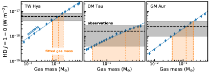
Figure 5: Gas mass ranges of TW Hya, DM Tau and GM Aur obtained by comparing model HD 1-0 integrated fluxes to the observations (Bergin et al., 2013; McClure et al., 2016). Observations are shown in black, with the gray shaded region showing the $3\sigma$ uncertainty. Blue points show individual model fluxes, to which we have fitted the power law shown as the blue dashed line. The orange vertical line and shaded region show the best fitting gas mass and $3\sigma$ uncertainty, respectively.

References

- Aikawa et al. (2015) Aikawa, Y., Furuya, K., Nomura, H., & Qi, C. 2015, ApJ, 807, 120, doi: 10.1088/0004-637X/807/2/120
- Aikawa et al. (1997) Aikawa, Y., Umebayashi, T., Nakano, T., & Miyama, S. M. 1997, ApJ, 486, L51
- Aikawa et al. (2021) Aikawa, Y., Cataldi, G., Yamato, Y., et al. 2021, ApJS, 257, 13, doi: 10.3847/1538-4365/ac143c
- Alarcón et al. (2020) Alarcón, F., Teague, R., Zhang, K., Bergin, E. A., & Barraza-Alfaro, M. 2020, ApJ, 905, 68, doi: 10.3847/1538-4357/abc1d6
- Anderson et al. (2019) Anderson, D. E., Blake, G. A., Bergin, E. A., et al. 2019, ApJ, 881, 127, doi: 10.3847/1538-4357/ab2cb5
- Andrews et al. (2011) Andrews, S. M., Wilner, D. J., Hughes, A., et al. 2011, ApJ, 744, 162
- Ansdell et al. (2016) Ansdell, M., Williams, J. P., van der Marel, N., et al. 2016, ApJ, 828, 46
- Astropy Collaboration et al. (2013) Astropy Collaboration, Robitaille, T. P., Tollerud, E. J., et al. 2013, A&A, 558, A33, doi: 10.1051/0004-6361/201322068
- Astropy Collaboration et al. (2018) Astropy Collaboration, Price-Whelan, A. M., Sipőcz, B. M., et al. 2018, AJ, 156, 123, doi: 10.3847/1538-3881/aabc4f
- Bergin et al. (2010) Bergin, E., Hogerheijde, M., Brinch, C., et al. 2010, A&A, 521, L33
- Bergin et al. (2016) Bergin, E. A., Du, F., Cleeves, L. I., et al. 2016, ApJ, 831, 101, doi: 10.3847/0004-637X/831/1/101
- Bergin et al. (2013) Bergin, E. A., Cleeves, L. I., Gorti, U., et al. 2013, Nature, 493, 644, doi: 10.1038/nature11805
- Bergner et al. (2019) Bergner, J. B., Öberg, K. I., Bergin, E. A., et al. 2019, ApJ, 876, 25, doi: 10.3847/1538-4357/ab141e
- Birnstiel et al. (2012) Birnstiel, T., Klahr, H., & Ercolano, B. 2012, A&A, 539, A148
- Booth et al. (2019) Booth, A. S., Walsh, C., Ilee, J. D., et al. 2019, ApJ, 882, L31, doi: 10.3847/2041-8213/ab3645
- Bosman et al. (2018) Bosman, A. D., Walsh, C., & van Dishoeck, E. F. 2018, A&A, 618, A182, doi: 10.1051/0004-6361/201833497
- Brickhouse et al. (2010) Brickhouse, N. S., Cranmer, S. R., Dupree, A. K., Luna, G. J. M., & Wolk, S. 2010, ApJ, 710, 1835, doi: 10.1088/0004-637X/710/2/1835
- Bruderer (2013) Bruderer, S. 2013, A&A, 559, A46, doi: 10.1051/0004-6361/201321171
- Bruderer et al. (2012) Bruderer, S., van Dishoeck, E. F., Doty, S. D., & Herczeg, G. J. 2012, A&A, 541, A91, doi: 10.1051/0004-6361/201118218
- Calahan et al. (2021) Calahan, J. K., Bergin, E., Zhang, K., et al. 2021, ApJ, 908, 8, doi: 10.3847/1538-4357/abd255
- Cleeves et al. (2015) Cleeves, L. I., Bergin, E. A., Qi, C., Adams, F. C., & Öberg, K. I. 2015, ApJ, 799, 204, doi: 10.1088/0004-637X/799/2/204
- Cleeves et al. (2018) Cleeves, L. I., Öberg, K. I., Wilner, D. J., et al. 2018, ApJ, 865, 155, doi: 10.3847/1538-4357/aade96
- Dionatos et al. (2019) Dionatos, O., Woitke, P., Güdel, M., et al. 2019, A&A, 625, A66, doi: 10.1051/0004-6361/201832860
- Favre et al. (2013) Favre, C., Cleeves, L. I., Bergin, E. A., Qi, C., & Blake, G. A. 2013, ApJ, 776, L38, doi: 10.1088/2041-8205/776/2/L38
- Furuya & Aikawa (2014) Furuya, K., & Aikawa, Y. 2014, ApJ, 790, 97, doi: 10.1088/0004-637X/790/2/97
- Gaia Collaboration et al. (2018) Gaia Collaboration, Brown, A. G. A., Vallenari, A., et al. 2018, A&A, 616, A1, doi: 10.1051/0004-6361/201833051
- Harris et al. (2020) Harris, C. R., Millman, K. J., van der Walt, S. J., et al. 2020, Nature, 585, 357
- Helled et al. (2014) Helled, R., Bodenheimer, P., Podolak, M., et al. 2014, in Protostars and Planets VI, ed. H. Beuther, R. S. Klessen, C. P. Dullemond, & T. Henning, 643, doi: 10.2458/azu_uapress_9780816531240-ch028
- Henning et al. (2010) Henning, T., Semenov, D., Guilloteau, S., et al. 2010, ApJ, 714, 1511, doi: 10.1088/0004-637X/714/2/1511
- Huang & Öberg (2015) Huang, J., & Öberg, K. I. 2015, ApJ, 809, L26, doi: 10.1088/2041-8205/809/2/L26
- Hunter (2007) Hunter, J. D. 2007, Computing in science & engineering, 9, 90
- Kama et al. (2016) Kama, M., Bruderer, S., van Dishoeck, E. F., et al. 2016, A&A, 592, A83, doi: 10.1051/0004-6361/201526991
- Kama et al. (2020) Kama, M., Trapman, L., Fedele, D., et al. 2020, A&A, 634, A88, doi: 10.1051/0004-6361/201937124
- Kenyon & Hartmann (1987) Kenyon, S. J., & Hartmann, L. 1987, ApJ, 323, 714, doi: 10.1086/165866
- Kim & Turner (2020) Kim, S. Y., & Turner, N. J. 2020, ApJ, 889, 159, doi: 10.3847/1538-4357/ab66ae
- Krijt et al. (2020) Krijt, S., Bosman, A. D., Zhang, K., et al. 2020, ApJ, 899, 134, doi: 10.3847/1538-4357/aba75d
- Krijt et al. (2018) Krijt, S., Schwarz, K. R., Bergin, E. A., & Ciesla, F. J. 2018, ApJ, 864, 78, doi: 10.3847/1538-4357/aad69b
- Long et al. (2017) Long, F., Herczeg, G. J., Pascucci, I., et al. 2017, ApJ, 844, 99
- McClure et al. (2016) McClure, M. K., Bergin, E. A., Cleeves, L. I., et al. 2016, ApJ, 831, 167, doi: 10.3847/0004-637X/831/2/167
- Miotello et al. (2014) Miotello, A., Bruderer, S., & van Dishoeck, E. F. 2014, A&A, 572, A96, doi: 10.1051/0004-6361/201424712
- Miotello et al. (2016) Miotello, A., van Dishoeck, E. F., Kama, M., & Bruderer, S. 2016, A&A, 594, A85, doi: 10.1051/0004-6361/201628159
- Miotello et al. (2017) Miotello, A., van Dishoeck, E. F., Williams, J. P., et al. 2017, A&A, 599, A113, doi: 10.1051/0004-6361/201629556
- Mordasini (2018) Mordasini, C. 2018, Planetary Population Synthesis, 143, doi: 10.1007/978-3-319-55333-7_143
- Oberg et al. (2021) Oberg, K. I., Guzman, V. V., Walsh, C., et al. 2021, arXiv e-prints, arXiv:2109.06268. https://arxiv.org/abs/2109.06268
- Qi et al. (2015) Qi, C., Öberg, K. I., Andrews, S. M., et al. 2015, ApJ, 813, 128, doi: 10.1088/0004-637X/813/2/128
- Qi et al. (2013) Qi, C., Öberg, K. I., Wilner, D. J., et al. 2013, Science, 341, 630, doi: 10.1126/science.1239560
- Qi et al. (2019) Qi, C., Öberg, K. I., Espaillat, C. C., et al. 2019, ApJ, 882, 160, doi: 10.3847/1538-4357/ab35d3
- Salinas et al. (2016) Salinas, V. N., Hogerheijde, M. R., Bergin, E. A., et al. 2016, A&A, 591, A122, doi: 10.1051/0004-6361/201628172
- Schwarz et al. (2016) Schwarz, K. R., Bergin, E. A., Cleeves, L. I., et al. 2016, ApJ, 823, 91, doi: 10.3847/0004-637X/823/2/91
- Schwarz et al. (2018) —. 2018, ApJ, 856, 85, doi: 10.3847/1538-4357/aaae08
- Schwarz et al. (2019) —. 2019, ApJ, 877, 131, doi: 10.3847/1538-4357/ab1c5e
- Schwarz et al. (2021) Schwarz, K. R., Calahan, J. K., Zhang, K., et al. 2021, ApJS, 257, 20, doi: 10.3847/1538-4365/ac143b
- Seifert et al. (2021) Seifert, R. A., Cleeves, L. I., Adams, F. C., & Li, Z.-Y. 2021, ApJ, 912, 136, doi: 10.3847/1538-4357/abf09a
- Thi et al. (2010) Thi, W.-F., Mathews, G., Ménard, F., et al. 2010, A&A, 518, L125, doi: 10.1051/0004-6361/201014578
- Toomre (1964) Toomre, A. 1964, ApJ, 139, 1217, doi: 10.1086/147861
- Trapman et al. (2017) Trapman, L., Miotello, A., Kama, M., van Dishoeck, E. F., & Bruderer, S. 2017, A&A, 605, A69, doi: 10.1051/0004-6361/201630308
- van Dishoeck & Black (1988) van Dishoeck, E. F., & Black, J. H. 1988, ApJ, 334, 771, doi: 10.1086/166877
- van ’t Hoff et al. (2017) van ’t Hoff, M. L. R., Walsh, C., Kama, M., Facchini, S., & van Dishoeck, E. F. 2017, A&A, 599, A101, doi: 10.1051/0004-6361/201629452
- van Zadelhoff et al. (2001) van Zadelhoff, G. J., van Dishoeck, E. F., Thi, W. F., & Blake, G. A. 2001, A&A, 377, 566, doi: 10.1051/0004-6361:20011137
- Visser et al. (2009) Visser, R., van Dishoeck, E. F., & Black, J. H. 2009, A&A, 503, 323, doi: 10.1051/0004-6361/200912129
- Williams & Best (2014) Williams, J. P., & Best, W. M. J. 2014, ApJ, 788, 59, doi: 10.1088/0004-637X/788/1/59
- Yu et al. (2017) Yu, M., Evans, Neal J., I., Dodson-Robinson, S. E., Willacy, K., & Turner, N. J. 2017, ApJ, 841, 39, doi: 10.3847/1538-4357/aa6e4c
- Yu et al. (2016) Yu, M., Willacy, K., Dodson-Robinson, S. E., Turner, N. J., & Evans, Neal J., I. 2016, ApJ, 822, 53, doi: 10.3847/0004-637X/822/1/53
- Zhang et al. (2017) Zhang, K., Bergin, E. A., Blake, G. A., Cleeves, L. I., & Schwarz, K. R. 2017, Nature Astronomy, 1, 0130, doi: 10.1038/s41550-017-0130
- Zhang et al. (2019) Zhang, K., Bergin, E. A., Schwarz, K., Krijt, S., & Ciesla, F. 2019, ApJ, 883, 98, doi: 10.3847/1538-4357/ab38b9
- Zhang et al. (2021) Zhang, K., Booth, A. S., Law, C. J., et al. 2021, ApJS, 257, 5, doi: 10.3847/1538-4365/ac1580