AutoMC: Automated Model Compression based on Domain Knowledge and Progressive search strategy
Abstract
Model compression methods can reduce model complexity on the premise of maintaining acceptable performance, and thus promote the application of deep neural networks under resource constrained environments. Despite their great success, the selection of suitable compression methods and design of details of the compression scheme are difficult, requiring lots of domain knowledge as support, which is not friendly to non-expert users. To make more users easily access to the model compression scheme that best meet their needs, in this paper, we propose AutoMC, an effective automatic tool for model compression. AutoMC builds the domain knowledge on model compression to deeply understand the characteristics and advantages of each compression method under different settings. In addition, it presents a progressive search strategy to efficiently explore pareto optimal compression scheme according to the learned prior knowledge combined with the historical evaluation information. Extensive experimental results show that AutoMC can provide satisfying compression schemes within short time, demonstrating the effectiveness of AutoMC.
1 Introduction
Neural networks are very powerful and can handle many real-world tasks, but their parameter amounts are generally very large bring expensive computation and storage cost. In order to apply them to mobile devices building more intelligent mobile devices, many model compression methods have been proposed, including model pruning [5, 21, 8, 2, 15], knowledge distillation [27], low rank approximation [2, 14] and so on.
These compression methods can effectively reduce model parameters while maintaining model accuracy as much as possible, but are difficult to use. Each method has many hyperparameters that can affect its compression effect, and different methods may suit for different compression tasks. Even the domain experts need lots of time to test and analyze for designing a reasonable compression scheme for a given compression task. This brings great challenges to the practical application of compression techniques.
In order to enable ordinary users to easily and effectively use the existing model compression techniques, in this paper, we propose AutoMC, an Automatic Machine Learning (AutoML) algorithm to help users automatically design model compression schemes. Note that in AutoMC, we do not limit a compression scheme to only use a compression method under a specific setting. Instead, we allow different compression methods and methods under different hyperparameters settings to work together (execute sequentially) to obtain diversified compression schemes. We try to integrate advantages of different methods/settings through this sequential combination so as to obtain more powerful compression effect, and our final experimental results prove this idea to be effective and feasible.
However, the search space of AutoMC is huge. The number of compression strategies111In this paper, a compression strategy refers to a compression method with a specific hyperparameter setting. contained in the compression scheme may be of any size, which brings great challenges to the subsequent search tasks. In order to improve the search efficiency, we present the following two innovations to improve the performance of AutoMC from the perspectives of knowledge introduction and search space reduction, respectively.
Specifically, for the first innovation, we built domain knowledge on model compression, which discloses the technical and settings details of compression strategies, and their performance under some common compression tasks. This domain knowledge can assist AutoMC to deeply understand the potential characteristics and advantages of each component in the search space. It can guide AutoMC select more appropriate compression strategies to build effective compression schemes, and thus reduce useless evaluation and improve the search efficiency.
As for the second innovation, we adopted the idea of progressive search space expansion to improve the search efficiency of AutoMC. Specifically, in each round of optimization, we only take the next operations, i.e., unexplored next-step compression strategies, of the evaluated compression scheme as the search space. Then, we select the pareto optimal operations for scheme evaluation, and finally take the next operations of the new scheme as the newly expanded search area to participate in the next round of optimization. In this way, AutoMC can selectively and gradually explore more valuable search space, reduce the search difficulty, and improve the search efficiency. In addition, AutoMC can analyze and compare the impact of subsequent operations on the performance of each compression scheme in a fine-grained manner, and finalize a more valuable next-step exploration route for implementation, thereby effectively reducing the evaluation of useless schemes.
The final experimental results show that AutoMC can quickly search for powerful model compression schemes. Compared with the existing AutoML algorithms which are non-progressive and ignore domain knowledge, AutoMC is more suitable for dealing with the automatic model compression problem where search space is huge and components are complete and executable algorithms.
Our contributions are summarized as follows:
-
1.
Automation. AutoMC can automatically design the effective model compression scheme according to the user demands. As far as we know, this is the first automatic model compression tool.
-
2.
Innovation. In order to improve the search efficiency of AutoMC algorithm, an effective analysis method based on domain knowledge and a progressive search strategy are designed. As far as we know, AutoMC is the first AutoML algorithm that introduce external knowledge.
-
3.
Effectiveness. Extensive experimental results show that with the help of domain knowledge and progressive search strategy, AutoMC can efficiently search the optimal model compression scheme for users, outperforming compression methods designed by humans.
2 Related Work
2.1 Model Compression Methods
Model compression is the key point of applying neural networks to mobile or embedding devices, and has been widely studied all over the world. Researchers have proposed many effective compression methods, and they can be roughly divided into the following four categories. (1) pruning methods, which aim to remove redundant parts e.g., filters, channels, kernels or layers, from the neural network [17, 7, 22, 18]; (2) knowledge distillation methods that train the compact and computationally efficient neural model with the supervision from well-trained larger models; (3) low-rank approximation methods that split the convolutional matrices into small ones using decomposition techniques [16]; (4) quantization methods that reduce the precision of parameter values of the neural network [10, 29].
These compression methods have their own advantages, and have achieved great success in many compression tasks, but are difficult to apply as is discussed in the introduction part. In this paper, we aim to flexibly use the experience provided by them to support the automatic design of model compression schemes.
2.2 Automated Machine Learning Algorithms
The goal of Automated Machine Learning (AutoML) is to realize the progressive automation of ML, including automatic design of neural network architecture, ML workflow [9, 28] and automatic setting of hyperparameters of ML model [23, 11]. The idea of the existing AutoML algorithms is to define an effective search space which contains a variety of solutions, then design an efficient search strategy to quickly find the best ML solution from the search space, and finally take the best solution as the final output.
Search strategy has a great impact on the performance of the AutoML algorithm. The existing AutoML search strategies can be divided into 3 categories: Reinforcement Learning (RL) methods [1], Evolutionary Algorithm (EA) based methods [4, 25] and gradient-based methods [24, 20]. The RL-based methods use a recurrent network as controller to determine a sequence of operators, thus construct the ML solution sequentially. EA-based methods initialize a population of ML solutions first and then evolve them with their validation accuracies as fitnesses. As for the gradient-based methods, they are designed for neural architecture search problems. They relax the search space to be continuous, so that the architecture can be optimized with respect to its validation performance by gradient descent [3]. They fail to deal with the search space composed of executable compression strategies. Therefore, we only compare AutoMC’s search strategy with the previous two methods.
| Label | Compression Method | Techniques | Hyperparameters | ||||||||||
| C1 | LMA [27] | : Knowledge distillation based on LMA function |
|
||||||||||
| C2 | LeGR [5] |
|
|
||||||||||
| C3 | NS [21] |
|
|
||||||||||
| C4 | SFP [8] | : Filter pruning based on back-propagation |
|
||||||||||
| C5 | HOS [2] |
|
|
||||||||||
| C6 | LFB [14] | : low-rank filter approximation based on filter basis |
|
3 Our Approach
We firstly give the related concepts on model compression and problem definition of automatic model compression (Section 3.1). Then, we make full use of the existing experience to construct an efficient search space for the compression area (Section 3.2). Finally, we designed a search strategy, which improves the search efficiency from the perspectives of knowledge introduction and search space reduction, to help users quickly search for the optimal compression scheme (Section 3.3).
3.1 Related Concepts and Problem Definition
Related Concepts. Given a neural model , we use , and to denote its parameter amount, FLOPS and its accuracy score on the given dataset, respectively. Given a model compression scheme , where is a compression strategy ( compression strategies are required to be executed in sequence), we use to denote the compressed model obtained after applying to . In addition, we use , where can be or , to represent model ’s reduction rate on parameter amount or FLOPS after executing . We use to represent accuracy increase rate achieved by on .
Definition 1 (Automatic Model Compression). Given a neural model , a target reduction rate of parameters and a search space on compression schemes, the Automatic Model Compression problem aims to quickly find :
| (1) |
A Pareto optimal compression scheme that performs well on two optimization objectives: and , and meets the target reduction rate of parameters.
3.2 Search Space on Compression Schemes
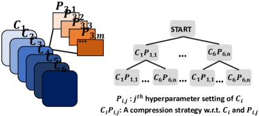
In AutoMC, we utilize some open source model compression methods to build a search space on model compression. Specifically, we collect 6 effective model compression methods, allowing them to be combined flexibly to obtain diverse model compression schemes to cope with different compression tasks. In addition, considering that hyperparameters have great impact on the performance of each method, we regard the compression method under different hyperparameter settings as different compression strategies, and intend to find the best compression strategy sequence, that is, the compression scheme, to effectively solve the actual compression problems.
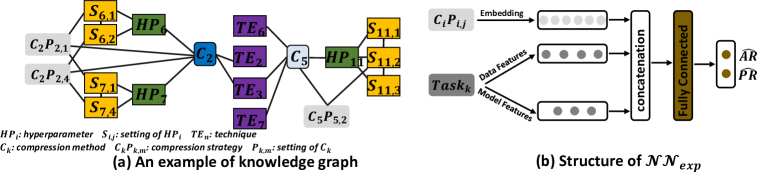
Table 1 gives these compression methods. These methods and their respective hyperparameters constitute a total of compression strategies. Utilizing these compression strategies to form compression strategy sequences of different lengths (length ), then we get a search space with different compression schemes.
Our search space can be described as a tree structure (as is shown in Figure 1), where each node (layer ) has child nodes corresponding to compression strategies and nodes at layer are leaf nodes. In this tree structure, each path from node to any node in the tree corresponds to a compression strategy sequence, namely a compression scheme in the search space.
3.3 Search Strategy of AutoMC Algorithm
The search space is huge. In order to improve the search performance, we introduce domain knowledge to help AutoMC learn characteristics of components of (Section 3.3.1). In addition, we design a progressive search strategy to finely analyze the impact of subsequent operations on the compression scheme, and thus improve search efficiency (Section 3.3.2).
3.3.1 Domain Knowledge based Embedding Learning
We build a knowledge graph on compression strategies, and extract experimental experience from the related research papers to learn potential advantages and effective representation of each compression strategy in the search space. Considering that two kinds of knowledge are of different types222knowledge graph is relational knowledge whereas experimental experience belongs to numerical knowledge and are suitable for different analytical methods, we design different embedding learning methods for them, and combine two methods for better understanding of different compression strategies.
Knowledge Graph based Embedding Learning. We build a knowledge graph that exposes the technical and settings details of each compression strategy, to help AutoMC to learn relations and differences between different compression strategies. contains five types of entity nodes: () compression strategy, () compression method, () hyperparameter, () hyperparameter’s setting and () compression technique. Also, it includes five types of entity relations:
-
:
corresponding relation between a compression strategy and its compression method ()
-
:
corresponding relation between a compression strategy and its hyperparameter setting ()
-
:
corresponding relation between a compression method and its hyperparameter ()
-
:
corresponding relation between a compression method and its compression technique ( )
-
:
corresponding relation between a hyperparameter and its setting ()
and describe the composition details of compression strategies, and provide a brief description of compression methods, illustrate the meaning of hyperparameter settings. Figure 2 (a) is an example of .
We use TransR [19] to effectively parameterize entities and relations in as vector representations, while preserving the graph structure of . Specifically, given a triplet in , we learn embedding of each entity and relation by optimizing the translation principle:
| (2) |
where and are the embedding for , , and respectively; is the transformation matrix of relation .
This embedding learning method can inject the knowledge in into representations of compression strategies, so as to learn effective representations of compression strategies. In AutoMC, we denote the embedding of compression strategy learned from by .
Experimental Experience based Embedding Enhancement. Research papers contain many valuable experimental experiences: the performance of compression strategies under a variety of compression tasks. These experiences are helpful for deeply understanding performance characteristics of each compression strategy. If we can integrate them into embeddings of compression strategies, then AutoMC can make more accurate decisions under the guidance of higher-quality embeddings.
Based on this idea, we design a neural network, which is denoted by (as shown in Figure 2 (b)), to further optimize the embeddings of compression strategies learned from . takes and the feature vector of a compression task (denoted by ) as input, intending to output ’s compression performance, including parameter’s reduction rate , and accuracy’s increase rate , on .
Here, is composed of dataset attributes and model performance information. Taking the compression task on image classification model as an example, the feature vector can be composed of the following 7 parts: (1) Data Features: category number, image size, image channel number and data amount. (2) Model Features: original model’s parameter amount, FLOPs, accuracy score on the dataset.
In AutoMC, we extract experimental experience from relevant compression papers: , then input and to to obtain the predicted performance scores, denoted by . Finally, we optimize and obtain a more effective embedding of , which is denoted by , by minimizing the differences between and :
| (3) |
where indicates the parameters of , represents the set of compression strategies in Table 1, and is the set of experimental experience extracted from papers.
Pseudo code. Combining the above two learning methods, then AutoMC can comprehensively consider knowledge graph and experimental experience and obtain a more effective embeddings. Algorithm 1 gives the complete pseudo code of the embedding learning part of AutoMC.
3.3.2 Progressive Search Strategy
Taking the compression scheme as the unit to analyze and evaluate during the search phase can be very inefficient, since the compression scheme evaluation can be very expensive when its sequence is long. The search strategy may cost much time on evaluation while only obtain less performance information for optimization, which is ineffective.
To improve search efficiency, we apply the idea of progressive search strategy instead in AutoMC. We try to gradually add the valuable compression strategy to the evaluated compression schemes by analyzing rich procedural information, i.e., the impact of each compression strategy on the original compression strategy sequence, so as to quickly find better schemes from the huge search space .
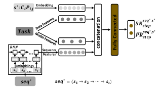
Specifically, we propose to utilize historical procedural information to learn a multi-objective evaluator (as shown in Figure 3). We use to analyze the impact of a newly added compression strategy on the performance of compression scheme , including the accuracy improvement rate and reduction rate of parameters .
For each round of optimization, we firstly sample some Pareto-Optimal and evaluated schemes , take their next-step compression strategies as the search space : , where are the sampled schemes. Secondly, use to select pareto optimal options from , thus obtain better compression schemes for evaluation.
| (4) |
where and are performance changes that brings to scheme predicted by . and are accuracy and parameter amount obtained after executing scheme to the original model .
Finally, we evaluate compression schemes in and get their real performance changes, which are denoted by , , and use the following formula to further optimize the performance of :
| (5) |
We add the new scheme to to participate in the next round of optimization steps.
Advantages of Progressive Search and AutoMC. In this way, AutoMC can obtain more training data for strategy optimization, and can selectively explore more valuable search space, thus improve the search efficiency.
Applying embeddings learned by Algorithm 1 to Algorithm 2, i.e., using the learned high-level embeddings to represent compression strategies and previous strategy sequences that need to input to , then we get AutoMC.
| PR(%) | Algorithm | ResNet-56 on CIFAR-10 | VGG-16 on CIFAR-100 | ||||
| Params(M) / PR(%) | FLOPs(G) / FR(%) | Acc. / Inc.(%) | Params(M) / PR(%) | FLOPs(G) / FR(%) | Acc. / Inc.(%) | ||
| baseline | 0.90 / 0 | 0.27 / 0 | 91.04 / 0 | 14.77 / 0 | 0.63 / 0 | 70.03 / 0 | |
| 40 | LMA | 0.53 / 41.74 | 0.15 / 42.93 | 79.61 / -12.56 | 8.85 / 40.11 | 0.38 / 40.26 | 42.11 / -39.87 |
| LeGR | 0.54 / 40.02 | 0.20 / 25.76 | 90.69 / -0.38 | 8.87 / 39.99 | 0.56 / 11.55 | 69.97 / -0.08 | |
| NS | 0.54 / 40.02 | 0.12 / 55.68 | 89.19 / -2.03 | 8.87 / 40.00 | 0.42 / 33.71 | 70.01 / -0.03 | |
| SFP | 0.55 / 38.52 | 0.17 / 36.54 | 88.24 / -3.07 | 8.90 / 39.73 | 0.38 / 39.31 | 69.62 / -0.58 | |
| HOS | 0.53 / 40.97 | 0.15 / 42.55 | 90.18 / -0.95 | 8.87 / 39.99 | 0.38 / 39.51 | 64.34 / -8.12 | |
| LFB | 0.54 / 40.19 | 0.14 / 46.12 | 89.99 / -1.15 | 9.40 / 36.21 | 0.04 / 93.00 | 60.94 / -13.04 | |
| Evolution | 0.45 / 49.87 | 0.14 / 48.83 | 91.77 / 0.80 | 8.11 / 45.11 | 0.36 / 42.54 | 69.03 / -1.43 | |
| AutoMC | 0.55 / 39.17 | 0.18 / 31.61 | 92.61 / 1.73 | 8.18 / 44.67 | 0.42 / 33.23 | 70.73 / 0.99 | |
| RL | 0.20 / 77.69 | 0.07 / 75.09 | 87.23 / -4.18 | 8.11 / 45.11 | 0.44 / 29.94 | 63.23 / -9.70 | |
| Random | 0.22 / 75.95 | 0.06 / 77.18 | 79.50 / -12.43 | 8.10 / 45.15 | 0.33 / 47.80 | 68.45 / -2.25 | |
| 70 | LMA | 0.27 / 70.40 | 0.08 / 72.09 | 75.25 / -17.35 | 4.44 / 69.98 | 0.19 / 69.90 | 41.51 / -40.73 |
| LeGR | 0.27 / 70.03 | 0.16 / 41.56 | 85.88 / -5.67 | 4.43 / 69.99 | 0.45 / 28.35 | 69.06 / -1.38 | |
| NS | 0.27 / 70.05 | 0.06 / 78.77 | 85.73 / -5.83 | 4.43 / 70.01 | 0.27 / 56.77 | 68.98 / -1.50 | |
| SFP | 0.29 / 68.07 | 0.09 / 67.24 | 86.94 / -4.51 | 4.47 / 69.72 | 0.19 / 69.22 | 68.15 / -2.68 | |
| HOS | 0.28 / 68.88 | 0.10 / 63.31 | 89.28 / -1.93 | 4.43 / 70.05 | 0.22 / 64.29 | 62.66 / -10.52 | |
| LFB | 0.27 / 70.03 | 0.08 / 71.96 | 90.35 / -0.76 | 6.27 / 57.44 | 0.03 / 95.2 | 57.88 / -17.35 | |
| Evolution | 0.44 / 51.47 | 0.10 / 63.66 | 89.21 / -2.01 | 4.14 / 72.01 | 0.22 / 64.30 | 60.47 / -13.64 | |
| AutoMC | 0.28 / 68.43 | 0.10 / 62.44 | 92.18 / 1.25 | 4.19 / 71.67 | 0.32 / 49.31 | 70.10 / 0.11 | |
| RL | 0.44 / 51.52 | 0.10 / 63.15 | 88.30 / -3.01 | 4.20 / 71.60 | 0.19 / 69.08 | 51.20 / -27.13 | |
| Random | 0.43 / 51.98 | 0.13 / 52.53 | 88.36 / -2.94 | 5.03 / 65.94 | 0.28 / 55.37 | 51.76 / -25.87 | |
| Algorithm | ResNet-20 on CIFAR-10 | ResNet-56 on CIFAR-10 | ResNet-164 on CIFAR-10 | VGG-13 on CIFAR-100 | VGG-16 on CIFAR-100 | VGG-19 on CIFAR-100 |
| LMA | 41.74 / 42.84 / 77.61 | 41.74 / 42.93 / 79.61 | 41.74 / 42.96 / 58.21 | 40.07 / 40.29 / 47.16 | 40.11 / 40.26 / 42.11 | 40.12 / 40.25 / 40.02 |
| LeGR | 39.86 / 21.20 / 89.20 | 40.02 / 25.76 / 90.69 | 39.99 / 33.11 / 83.93 | 40.00 / 12.15 / 70.80 | 39.99 / 11.55 / 69.97 | 39.99 / 11.66 / 69.64 |
| NS | 40.05 / 44.12 / 88.78 | 40.02 / 55.68 / 89.19 | 39.98 / 51.13 / 83.84 | 40.01 / 31.19 / 70.48 | 40.00 / 33.71 / 70.01 | 40.00 / 41.34 / 69.34 |
| SFP | 38.30 / 35.49 / 87.81 | 38.52 / 36.54 / 88.24 | 38.58 / 36.88 / 82.06 | 39.68 / 39.16 / 70.69 | 39.73 / 39.31 / 69.62 | 39.76 / 39.40 / 69.42 |
| HOS | 40.12 / 39.66 / 88.81 | 40.97 / 42.55 / 90.18 | 41.16 / 43.50 / 84.12 | 40.06 / 39.36 / 64.13 | 39.99 / 39.51 / 64.34 | 40.01 / 39.13 / 63.37 |
| LFB | 40.38 / 45.80 / 91.57 | 40.19 / 46.12 / 89.99 | 40.09 / 76.76 / 24.17 | 37.82 / 92.92 / 63.04 | 36.21 / 93.00 / 60.94 | 35.46 / 93.05 / 56.27 |
| Evolution | 49.50 / 46.66 / 89.95 | 49.87 / 48.83 / 91.77 | 49.95 / 49.44 / 87.69 | 45.15 / 35.58 / 62.95 | 45.11 / 42.54 / 69.03 | 45.19 / 36.64 / 63.30 |
| Random | 75.94 / 74.44 / 78.38 | 75.95 / 77.18 / 79.50 | 75.91 / 78.08 / 59.37 | 45.18 / 24.04 / 62.02 | 45.15 / 47.80 / 68.45 | 45.11 / 33.06 / 68.81 |
| RL | 77.87 / 69.05 / 84.28 | 77.69 / 75.09 / 87.23 | 77.23 / 83.27 / 74.21 | 45.20 / 26.00 / 62.36 | 45.11 / 29.94 / 63.23 | 45.14 / 38.78 / 68.31 |
| AutoMC | 38.73 / 30.00 / 91.42 | 39.17 / 31.61 / 92.61 | 39.30 / 40.76 / 88.50 | 44.60 / 34.43 / 71.77 | 44.67 / 33.23 / 70.73 | 44.68 / 35.09 / 70.56 |
4 Experiments
In this part, we examine the performance of AutoMC. We firstly compare AutoMC with human designed compression methods to analyze AutoMC’s application value and the rationality of its search space design (Section 4.2). Secondly, we compare AutoMC with classical AutoML algorithms to test the effectiveness of its search strategy (Section 4.3). Then, we transfer the compression scheme searched by AutoMC to other neural models to examine its transferability (Section 4.4). Finally, we conduct ablation studies to analyze the impact of embedded learning method based on domain knowledge and progressive search strategy on the overall performance of AutoMC (Section 4.5).
We implemented all algorithms using Pytorch and performed all experiments using RTX 3090 GPUs.
4.1 Experimental Setup
Compared Algorithms. We compare AutoMC with two popular search strategies for AutoML: a RL search strategy that combines recurrent neural network controller [6] and EA-based search strategy for multi-objective optimization [6], and a commonly used baseline in AutoML, Random Search. To enable these AutoML algorithms to cope with our automatic model compression problem, we set their search space to (). In addition, we take 6 state-of-the-art human-invented compression methods: LMA [27], LeGR [5], NS [21], SFP [8], HOS [2] and LFB [14], as baselines, to show the importance of automatic model compression.
Compression Tasks. We construct two experiments to examine the performance of AutoML algorithms. Exp1: =CIAFR-10, = ResNet-56, =0.3; Exp2: = CIAFR-100, =VGG-16, =0.3, where CIAFR-10 and CIAFR-100 [13] are two commonly used image classification datasets, and ResNet-56 and VGG-16 are two popular CNN network architecture.
To improve the execution speed, we sample 10% data from to execute AutoML algorithms in the experiments. After executing AutoML algorithms, we select the Pareto optimal compression scheme with for evaluation. As for the existing compression methods, we apply grid search to get their optimal hyperparameter settings and set their parameter reduction rate to 0.4 and 0.7 to analyze their compression performance.
Furthermore, to evaluate the transferability of compression schemes searched by AutoML algorithms, we design two transfer experiments. We transfer compression schemes searched on ResNet-56 to ResNet-20 and ResNet-164, and transfer schemes from VGG-16 to VGG-13 and VGG-19.
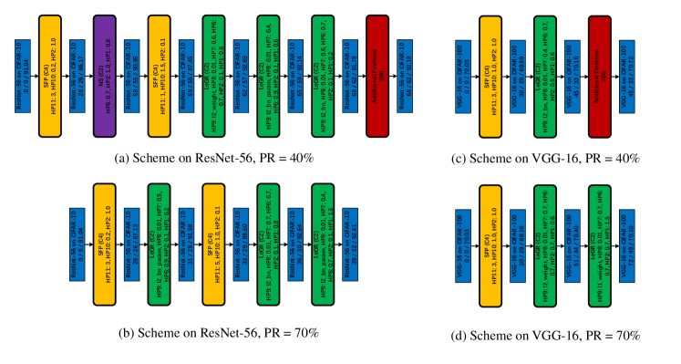
Implementation Details. In AutoMC, the embedding size is set to . and are trained with the Adam with a learning rate of 0.001. After AutoMC searches for 3 GPU days, we choose the Pareto optimal compression schemes as the final output. As for the compared AutoML algorithms, we follow implementation details reported in their papers, and control the running time of each AutoML algorithm to be the same. Figure 6 gives the best compression schemes searched by AutoMC.
4.2 Comparison with the Compression Methods
Table 2 gives the performance of AutoMC and the existing compression methods on different tasks. We can observe that compression schemes designed by AutoMC surpass the manually designed schemes in all tasks. These results prove that AutoMC has great application value. It has the ability to help users search for better compression schemes automatically to solve specific compression tasks.
In addition, the experimental results show us: (1) A compression strategy may performs better with smaller parameter reduction rate (). Taking result of ResNet-56 on CIFAR-10 using LeGR as an example, when the is 0.4, on average, the model performance falls by 0.0088% for every 1% fall in parameter amount; however, when becomes larger, the model performance falls by 0.0737% for every 1% fall in parameter amount. (2) Different compression strategies may be appropriate for different compression tasks. For example, LeGR performs better than HOS when the whereas HOS outperforms LeGR when . Based on the above two points, combination of multiple compression strategies and fine-grained compression for a given compression task may achieve better results. This is consistent with our idea of designing the AutoMC search space, and it further proves the rationality of the AutoMC search space design.
4.3 Comparison with the NAS algorithms
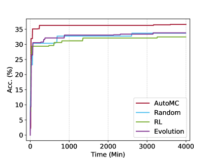
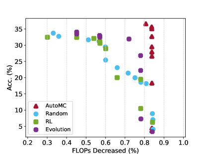
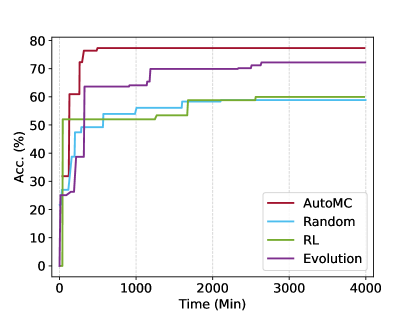
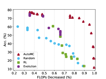
Table 2 gives the performance of different AutoML algorithms on different compression tasks. Figure 4 provides the performance of the best compression scheme (Pareto optimal scheme with highest accuracy score) and all Pareto optimal schemes searched by AutoML algorithms. We can observe that RL algorithm performs well in the very early stage, but its performance improvement is far behind other AutoML algorithms in the later stage. Evolution algorithm outperforms the other algorithms except AutoMC in both experiments. As for the Random algorithm, its performance have been rising throughout the entire process, but still worse than most algorithms. Compared with the existing AutoML algorithms, AutoMC can search for better model compression schemes more quickly, and is more suitable for the search space which contains a huge number of candidates. These results demonstrate the effectiveness of AutoMC and the rationality of its search strategy design.
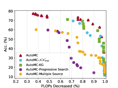
4.4 Tansfer Study
Table 3 shows the performance of different models transfered from ResNet-56 and VGG-16. We can observe that LFB outperforms AutoMC with ResNet-20 on CIFAR-10. We think the reason is that LFB has a talent for dealing with small models. It’s obvious that the performance of LFB gradually decreases as the scale of the model increases. For example, LFB achieves an accuracy of 91.57% with ResNet-20 on CIFAR-10, but only achieves 24.17% with ResNet-164 on CIFAR-10. Except that, compression schemes designed by AutoMC surpass the manually designed schemes in all tasks. These results prove that AutoMC has great transferability. It is able to help users search for better compression schemes automatically with models of different scales.
Besides, the experimental results show that the same compression strategies may achieve diferent performance on models of different scales. In addition to the example of LFB and AutoMC above, LeGR performs better than HOS when using ResNet-20 whereas HOS outperforms LeGR when using ResNet-164. Based the above, combination of multiple compression strategies and fine-grained compression for models of different scales may achieve more stable and competitive performance.
4.5 Ablation Study
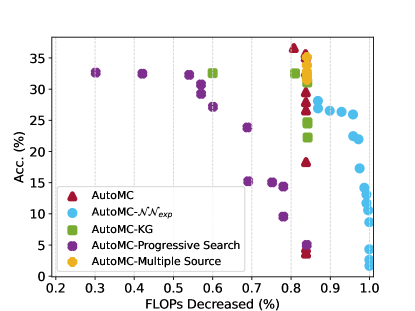
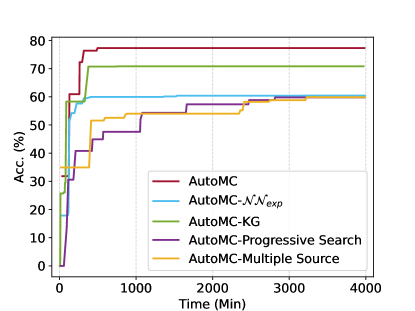
We further investigate the effect of the knowledge based embedding learning method, experience based embedding learning method and the progressive search strategy, three core components of our algorithm, on the performance of AutoMC using the following four variants of AutoMC, thus verify innovations presented in this paper.
-
1
AutoMC-KG. This version of AutoMC removes knowledge graph embedding method.
-
2
AutoMC-. This version of AutoMC removes experimental experience based embedding method.
-
3
AutoMC-Multiple Source. This version of AutoMC only uses strategies w.r.t. LeGR to construct search space.
-
4
AutoMC-Pregressive Search. This version of AutoMC replaces the progressive search strategy with the RL based search strategy that combines recurrent neural network.
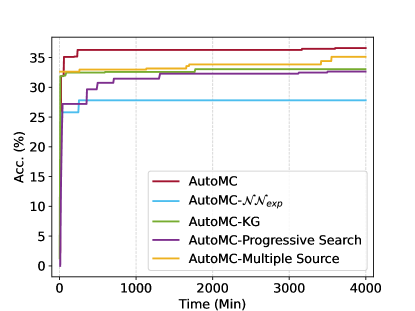
Corresponding results are shown in Figure 5, we can see that AutoMC has much better performance than AutoMC-KG and AutoMC-, which ignore the knowledge graph or experimental experience on compression strategies while learning their embedding. This result shows us the significance and necessity of fully considering two kinds of knowledge on compression strategies in the AutoMC, for effective embedding learning. Our proposed knowledge graph embedding method can explore the differences and linkages between compression strategies in the search space, and the experimental experience based embedding method can reveal the performance characteristics of compression strategies. Two embedding learning methods can complement each other and help AutoMC have a better and more comprehensive understanding of search space components.
Also, We notice that AutoMC-Multiple Source achieve worse performance than AutoMC. AutoMC-Multiple use only one compression method to complete compression tasks. The result indicates the importance of using multi-source compression strategies to build the search space.
Besides, we observe that AutoMC-Progressive Search performs much worse than AutoMC. RL’s unprogressive search process, i.e., only search for, evaluate, and analyze complete compression schemes, performs worse in the automatic compression scheme design problem task. It fails to effectively use historical evaluation details to improve the search effect and thus be less effective than AutoMC.
5 Conclusion
In this paper, we propose the AutoMC to automatically design optimal compression schemes according to the requirements of users. AutoMC innovatively introduces domain knowledge to assist search strategy to deeply understand the potential characteristics and advantages of each compression strategy, so as to design compression scheme more reasonably and easily. In addition, AutoMC presents the idea of progressive search space expansion, which can selectively explore valuable search regions and gradually improve the quality of the searched scheme through finer-grained analysis. This strategy can reduce the useless evaluations and improve the search efficiency. Extensive experimental results show that the combination of existing compression methods can create more powerful compression schemes, and the above two innovations make AutoMC more efficient than existing AutoML methods. In future works, we will try to enrich our search space, and design a more efficient search strategy to tackle this search space for further improving the performance of AutoMC.
References
- [1] Irwan Bello, Barret Zoph, Vijay Vasudevan, and Quoc V. Le. Neural optimizer search with reinforcement learning. In Doina Precup and Yee Whye Teh, editors, ICML, volume 70 of Proceedings of Machine Learning Research, pages 459–468. PMLR, 2017.
- [2] Christos Chatzikonstantinou, Georgios Th. Papadopoulos, Kosmas Dimitropoulos, and Petros Daras. Neural network compression using higher-order statistics and auxiliary reconstruction losses. In CVPR, pages 3077–3086, 2020.
- [3] Daoyuan Chen, Yaliang Li, Minghui Qiu, Zhen Wang, Bofang Li, Bolin Ding, Hongbo Deng, Jun Huang, Wei Lin, and Jingren Zhou. Adabert: Task-adaptive BERT compression with differentiable neural architecture search. In Christian Bessiere, editor, IJCAI, pages 2463–2469. ijcai.org, 2020.
- [4] Yukang Chen, Gaofeng Meng, Qian Zhang, Shiming Xiang, Chang Huang, Lisen Mu, and Xinggang Wang. RENAS: reinforced evolutionary neural architecture search. In CVPR, pages 4787–4796. Computer Vision Foundation / IEEE, 2019.
- [5] Ting-Wu Chin, Ruizhou Ding, Cha Zhang, and Diana Marculescu. Towards efficient model compression via learned global ranking. In CVPR, pages 1515–1525, 2020.
- [6] Yang Gao, Hong Yang, Peng Zhang, Chuan Zhou, and Yue Hu. Graph neural architecture search. In Christian Bessiere, editor, IJCAI, pages 1403–1409. ijcai.org, 2020.
- [7] Ariel Gordon, Elad Eban, Ofir Nachum, Bo Chen, Hao Wu, Tien-Ju Yang, and Edward Choi. Morphnet: Fast & simple resource-constrained structure learning of deep networks. In CVPR, pages 1586–1595. Computer Vision Foundation / IEEE Computer Society, 2018.
- [8] Yang He, Guoliang Kang, Xuanyi Dong, Yanwei Fu, and Yi Yang. Soft filter pruning for accelerating deep convolutional neural networks. In Jérôme Lang, editor, IJCAI, pages 2234–2240, 2018.
- [9] Yuval Heffetz, Roman Vainshtein, Gilad Katz, and Lior Rokach. Deepline: Automl tool for pipelines generation using deep reinforcement learning and hierarchical actions filtering. In Rajesh Gupta, Yan Liu, Jiliang Tang, and B. Aditya Prakash, editors, KDD, pages 2103–2113. ACM, 2020.
- [10] Benoit Jacob, Skirmantas Kligys, Bo Chen, Menglong Zhu, Matthew Tang, Andrew G. Howard, Hartwig Adam, and Dmitry Kalenichenko. Quantization and training of neural networks for efficient integer-arithmetic-only inference. In CVPR, pages 2704–2713. Computer Vision Foundation / IEEE Computer Society, 2018.
- [11] Aaron Klein, Zhenwen Dai, Frank Hutter, Neil D. Lawrence, and Javier Gonzalez. Meta-surrogate benchmarking for hyperparameter optimization. In Hanna M. Wallach, Hugo Larochelle, Alina Beygelzimer, Florence d’Alché-Buc, Emily B. Fox, and Roman Garnett, editors, NeurIPS, pages 6267–6277, 2019.
- [12] Tamara G. Kolda and Brett W. Bader. Tensor decompositions and applications. SIAM Rev., 51(3):455–500, 2009.
- [13] A. Krizhevsky and G. Hinton. Learning multiple layers of features from tiny images. Handbook of Systemic Autoimmune Diseases, 1(4), 2009.
- [14] Yawei Li, Shuhang Gu, Luc Van Gool, and Radu Timofte. Learning filter basis for convolutional neural network compression. In ICCV, pages 5622–5631, 2019.
- [15] Yuchao Li, Shaohui Lin, Baochang Zhang, Jianzhuang Liu, David S. Doermann, Yongjian Wu, Feiyue Huang, and Rongrong Ji. Exploiting kernel sparsity and entropy for interpretable CNN compression. In CVPR, pages 2800–2809, 2019.
- [16] Shaohui Lin, Rongrong Ji, Xiaowei Guo, and Xuelong Li. Towards convolutional neural networks compression via global error reconstruction. In Subbarao Kambhampati, editor, IJCAI, pages 1753–1759. IJCAI/AAAI Press, 2016.
- [17] Shaohui Lin, Rongrong Ji, Chenqian Yan, Baochang Zhang, Liujuan Cao, Qixiang Ye, Feiyue Huang, and David S. Doermann. Towards optimal structured CNN pruning via generative adversarial learning. In CVPR, pages 2790–2799. Computer Vision Foundation / IEEE, 2019.
- [18] Shaohui Lin, Rongrong Ji, Chenqian Yan, Baochang Zhang, Liujuan Cao, Qixiang Ye, Feiyue Huang, and David S. Doermann. Towards optimal structured CNN pruning via generative adversarial learning. In CVPR, pages 2790–2799. Computer Vision Foundation / IEEE, 2019.
- [19] Yankai Lin, Zhiyuan Liu, Maosong Sun, Yang Liu, and Xuan Zhu. Learning entity and relation embeddings for knowledge graph completion. In Blai Bonet and Sven Koenig, editors, AAAI, pages 2181–2187, 2015.
- [20] Hanxiao Liu, Karen Simonyan, and Yiming Yang. DARTS: differentiable architecture search. In ICLR. OpenReview.net, 2019.
- [21] Zhuang Liu, Jianguo Li, Zhiqiang Shen, Gao Huang, Shoumeng Yan, and Changshui Zhang. Learning efficient convolutional networks through network slimming. In ICCV, pages 2755–2763, 2017.
- [22] Zechun Liu, Haoyuan Mu, Xiangyu Zhang, Zichao Guo, Xin Yang, Kwang-Ting Cheng, and Jian Sun. Metapruning: Meta learning for automatic neural network channel pruning. In ICCV, pages 3295–3304. IEEE, 2019.
- [23] Masahiro Nomura, Shuhei Watanabe, Youhei Akimoto, Yoshihiko Ozaki, and Masaki Onishi. Warm starting CMA-ES for hyperparameter optimization. In AAAI, pages 9188–9196. AAAI Press, 2021.
- [24] Asaf Noy, Niv Nayman, Tal Ridnik, Nadav Zamir, Sivan Doveh, Itamar Friedman, Raja Giryes, and Lihi Zelnik. ASAP: architecture search, anneal and prune. In Silvia Chiappa and Roberto Calandra, editors, AISTATS, volume 108 of Proceedings of Machine Learning Research, pages 493–503. PMLR, 2020.
- [25] Esteban Real, Alok Aggarwal, Yanping Huang, and Quoc V. Le. Regularized evolution for image classifier architecture search. In AAAI, pages 4780–4789. AAAI Press, 2019.
- [26] M. Sanaullah. A review of higher order statistics and spectra in communication systems. Global Journal of Science Frontier Research, pages 31–50, 05 2013.
- [27] Zhenhui Xu, Guolin Ke, Jia Zhang, Jiang Bian, and Tie-Yan Liu. Light multi-segment activation for model compression. In AAAI, pages 6542–6549, 2020.
- [28] Anatoly Yakovlev, Hesam Fathi Moghadam, Ali Moharrer, Jingxiao Cai, Nikan Chavoshi, Venkatanathan Varadarajan, Sandeep R. Agrawal, Tomas Karnagel, Sam Idicula, Sanjay Jinturkar, and Nipun Agarwal. Oracle automl: A fast and predictive automl pipeline. Proc. VLDB Endow., 13(12):3166–3180, 2020.
- [29] Aojun Zhou, Anbang Yao, Yiwen Guo, Lin Xu, and Yurong Chen. Incremental network quantization: Towards lossless cnns with low-precision weights. In ICLR. OpenReview.net, 2017.