Probabilistic error cancellation with sparse Pauli-Lindblad models on noisy quantum processors

Noise in pre-fault-tolerant quantum computers can result in biased estimates of physical observables. Accurate bias-free estimates can be obtained using probabilistic error cancellation (PEC), which is an error-mitigation technique that effectively inverts well-characterized noise channels. Learning correlated noise channels in large quantum circuits, however, has been a major challenge and has severely hampered experimental realizations. Our work presents a practical protocol for learning and inverting a sparse noise model that is able to capture correlated noise and scales to large quantum devices. These advances allow us to demonstrate PEC on a superconducting quantum processor with crosstalk errors, thereby providing an important milestone in opening the way to quantum computing with noise-free observables at larger circuit volumes.

Introduction

As a result of continuous improvement in quantum hardware and control systems, quantum processors are now able to provide more qubits with longer coherence times and better gate fidelities zhang2020ibm ; arute2019 ; Wu2021 . Despite these improvements, the levels of noise in current quantum processors still limit the depth of quantum circuits and reduce the accuracy of measured observables. Nevertheless, there is a growing number of quantum applications that run on noisy quantum processors and still provide competitive results peruzzo2014variational ; kandala2017hardware ; KIM2021WYMa-arXiv ; havlivcek2019supervised ; schuld2019quantum . Fault tolerance using quantum error correction or similar techniques would solve many noise related issues, but until this is achieved, quantum error mitigation TEM2017BGa ; LiBenjamin2017 ; kandala2019error ; END2018BLa may very well be the best way forward. Unlike error correction, which ensures that quantum circuits can be executed faithfully, error mitigation only aims to produce accurate expectation values $\langle A\rangle$ of observables $A$.

One of the earliest and most general protocols for error mitigation is probabilistic error cancellation (PEC) TEM2017BGa . To implement the error mitigated action $\mathcal{U}(\rho)=U\rho\,U^{{\dagger}}$ of an ideal gate $U$ on a devices where only noisy operations ${\cal U}\circ\Lambda$ are available, the protocol first requires an accurate noise model $\Lambda$. The action of the ideal gate would then be obtained by applying the mathematical inverse $\Lambda^{-1}$ before the noisy gate. Although $\Lambda^{-1}$ is not a physical operation, it can be expressed as a linear combination of gates and state-preparation operations TEM2017BGa ; END2018BLa . The PEC protocol implements this linear combination on average by promoting it to a quasi-probability distribution. Sampling the distribution generates physical circuit instances and results in an expectation value $\langle\hat{A}_{N}\rangle$ that is unbiased and completely removes the effect of $\Lambda$. However, this comes at the expense of an increased sampling overhead we denote by $\gamma$, which captures the noise strength and the resulting increase of the standard deviation.

Despite the method’s theoretical appeal END2018BLa ; GUO2022Ya-arXiv ; PIV2021SWa-arXiv ; doi:10.7566/JPSJ.90.032001 ; piveteau2021error ; PhysRevResearch.3.033178 ; takagi2021fundamental , practical challenges have limited its demonstration to the one- and two-qubit level doi:10.1126/sciadv.aaw5686 ; Zha2020LZCa . The main difficulty has been the accurate representation of the noise in a full device, which is particularly complicated by cross-talk errors that occur during the parallel application of gates. This has lead to protocols where a quasi-probability distribution for mitigation is determined by minimizing the deviation of a set of measured and exact expectation values strikis2021learning . Fully scalable implementations of PEC require a noise model $\Lambda$ that accurately captures correlated errors across all qubits, has a compact representation that can be learned efficiently, and has an inverse representation that enables tractable sampling from the associated quasi-probability distribution.

We address these challenges in the context of quantum circuits that consist of $l$ layers of noisy two-qubit gates interleaved with layers of single-qubit gates. Each layer $i=1,\ldots,l$ consists of a noisy operator $\tilde{\mathcal{U}}_{i}$ and is error mitigated by $\Lambda_{i}^{-1}$, as shown in Fig. 1a. The noise channel $\Lambda_{i}$ is specific to the gates in layer $i$ and is assumed to be a Pauli channel. If needed, this can be ensured using Pauli twirling PhysRevLett.76.722 ; knill2004fault ; kern2005quantum ; geller2013efficient ; wallman2016noise , as illustrated in Figs. 1b and 1c for an example with four qubits and two cx gates.

We present an efficient mitigation scheme that models the noise across each layer of two-qubit gates as a sparse Pauli-Lindblad error model. In our experiments, the model includes only weight-one and weight-two Pauli terms whose support coincides with the quantum processor’s connectivity. The parameters of the resulting model scale linearly with the number of qubits, which ensures that the model is efficiently represented and easy to learn. The inverse noise model is obtained simply by negating the model coefficients and gives rise to a quasi-probability distribution on Pauli matrices. We provide an efficient algorithm for sampling this distribution in linear time with the number of model coefficients. The mitigation Paulis can be combined with those used for twirling as well as with the single-qubit operations in the interleaved layers. The error mitigation scheme therefore maintains the original circuit structure and changes only the classical distribution of the single-qubit gates.

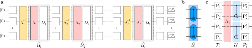
Fig. 1: Context of the noise model. (a) ideal error mitigation of a circuit consisting of $l$ layers of noisy two-qubit gates interleaved with layers of single-qubit gates. (b) example of a layer consisting of two noisy cx gates. (c) expansion of the same layer in terms of the ideal gates $\mathcal{U}_{i}$ and noise channel $\Lambda_{i}$, flanked with Pauli-twirl gates $\mathcal{P}_{i}$ and $\mathcal{P}_{i}^{\prime}=\mathcal{U}_{i}\mathcal{P}_{i}\mathcal{U}_{i}^{{\dagger}}$, where $\mathcal{P}_{i}$ is sampled uniformly at random.

Pauli-Lindblad noise model

We model a given $n$-qubit Pauli noise channel $\Lambda$ that arises from a sparse set of local interactions, according to a Lindblad Master equation BRE2002Pa with generator $\mathcal{L}(\rho)=\sum_{k\in\mathcal{K}}\lambda_{k}\big{(}P_{k}\rho P_{k}^{{\dagger}}-\rho\big{)}$, where $\mathcal{K}$ represents a set of local Paulis $P_{k}$ and $\lambda_{k}$ denotes the corresponding model coefficient. The resulting model is then given by (see Supplementary Materials Sec. SIII)

$$\Lambda(\rho)=\mbox{exp}[\mathcal{L}](\rho)=\prod_{k\in\mathcal{K}}\left(w_{k}\cdot+(1-w_{k})P_{k}\cdot P_{k}^{{\dagger}}\right)\rho,$$ (1)

where $w_{k}=2^{-1}(1+e^{-2\lambda_{k}})$. The model terms $\mathcal{K}$ are chosen to reflect the noise interactions in the quantum processor and their number, which determines the model complexity and expressivity, typically scales polynomially in $n$ and therefore allows us to represent noise models for the full device by a small set of nonnegative coefficients $\lambda_{k}$.

The fidelity of a Pauli matrix $P_{b}$ with respect to $\Lambda$ is given by $f_{b}=\frac{1}{2^{n}}\mathrm{Tr}\big{(}P_{b}^{{\dagger}}\Lambda(P_{b})\big{)}$. Defining the symplectic inner product $\langle b,k\rangle_{sp}$ to be $0$ if Paulis $P_{b}$ and $P_{k}$ commute and $1$ otherwise, we can concisely express the relationship between model coefficients $\lambda$ and the vector $f=\{f_{b}\}_{b\in\mathcal{B}}$ of fidelities for an arbitrary set of Paulis $\mathcal{B}$ as $\log(f)=-2M(\mathcal{B},\mathcal{K})\lambda$, where the logarithm is applied elementwise and the entries of binary matrix $M(\mathcal{B},\mathcal{K})$ are given by $M_{b,k}=\langle b,k\rangle_{sp}$. For a given $\lambda$ this allows us to evaluate the fidelity of any set of Paulis $\mathcal{B}$. More importantly, though, the relationship allows us to fit physical model parameters, $\lambda\geq 0$, given the fidelity estimates $\hat{f}$ for a set of benchmark Paulis $\mathcal{B}$ by solving a nonnegative least-squares problem in $\log(\hat{f})$; see Supplementary Materials Sec. SIII.3 for more details.

Various methods of learning the fidelities of Pauli channels are known FLA2020Wa ; ERH2019WPMa ; PhysRevX.4.011050 ; HEL2019XVWa and have been implemented experimentally harper2020efficient . The central idea in these methods is that the same noise process is repeated up to $d$ times and the corresponding Pauli expectation values are measured at every depth. The fidelities for the noise channel can then be extracted from the decay rates in the resulting curves in a way that is robust to state-preparation and measurement (SPAM) errors. In Supplementary Materials Sec. SIV.2 we provide theoretical guarantees for the sample complexity for learning the error model. Under mild conditions on the minimal fidelity of the noise channel and the level of SPAM errors we provide the following result for all the fidelities predicted by the model: Assume that the channel can be represented with the model Paulis from set $\mathcal{K}$, and that the channel fidelities for Paulis in $\mathcal{B}$ are learned by benchmarking up to depth $d$ with at least $2\epsilon^{-2}\log(2|\mathcal{B}|/\delta)$ circuit instances for each of the relevant measurement bases. Then it holds with probability at least $1-\delta$ that the estimates $\hat{f}_{j}$ of all fidelities $f_{j}$ are bounded by

$$C_{\epsilon}^{-\tau}\leq f_{j}\,\hat{f_{j}}^{-1}\leq C_{\epsilon}^{\tau},$$ (2)

with $\tau\!=\!\sqrt{|\mathcal{K}|\cdot|\mathcal{B}|}/(\sigma_{\min}(M(\mathcal{B},\mathcal{K}))d)$, and $C_{\epsilon}=\big{(}{\textstyle\frac{1+4\epsilon}{1-4\epsilon}}\big{)}$.

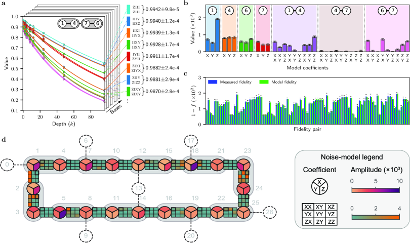
Fig. 2: Learning the noise channel. (a) The first step in learning our noise model, in this case for the four-qubit layer depicted in the top inset with two concurrent cx gates, is to measure a set of observables with increasing numbers of circuit repetitions $k$ (even) up to some maximum depth $d$. This requires measurements in nine different bases, illustrated by the stacked planes. Associated with each observable $P_{o}$ is a fidelity of the form $\alpha_{o}(f_{1}f_{2})^{k/2}$, where $\alpha_{o}$ is a constant that captures the state-preparation and measurement error, and $f_{1}$ and $f_{2}$ are the fidelities of the noise channel for two Pauli terms. We estimate the values of the different fidelity pairs in a consistent manner by fitting exponentially decaying curves through the data point of all observables that include the same pair, which may arise in multiple bases and possibly different observables, whose curves may have a different offset values $\alpha_{o}$. The legend on the right hand side illustrates the fidelity estimates for several pairs along with their standard deviation obtained using a 100-fold bootstrap (the error bars for the data points are small and largely covered by the markers). (b) Model coefficients obtained using a nonnegative least-squares fit of the log fidelities. (c) Plot of one minus the fidelity for each of the measured fidelity pairs including error bars representing the standard deviation (vertical lines in the error bars are omitted for clarity), along with the corresponding fidelities from the learned noise model. (d) Visualization of the sparse noise model of a 20-qubit layer with 10 concurrent cx gates (shaded pairs) overlaid on the topology of the ibm_hanoi quantum processor. Circles denote qubits (labeled by numbers); colored wedges in the circle visualize the single-body $X,Y$, and $Z$ Lindblad coefficients (see legend top). Two-body coefficients, e.g. $XX$, for adjacent qubit pairs are visually represented by a $3\times 3$ matrix (see legend bottom). The first Pauli character corresponds to the qubit adjacent the highlighted tile.

Experimental model fitting

To illustrate the learning protocol, we first benchmark the four-qubit layer with two cx gates shown in Figure 1b on a 27-transmon-qubit, fixed-connectivity processor with a heavy-hex topology, with qubits as indicated at the top of Fig. 2a. For all our experiments we apply dynamical decoupling sequences during idle times of qubits in the layer. These idle times arise when one or more gates in the layer are significantly faster than the slowest one, or when a qubit in the layer does not contain a gate (see also Supplementary Materials Sec. SVII.3). Repeated application of a noise channel in the context of self-adjoint two-qubit Clifford gates, such as cx and cz gates, generally results in pairwise products of fidelities. Although inserting appropriate single-qubit gates between applications can increase the number of individual Pauli fidelities estimates, pairwise fidelities will always remain, leading to indeterminacy of model coefficients; for instance, we can express the pairwise fidelity $f_{a}f_{b}$ as $(\alpha f_{a})(f_{b}/\alpha)$ for any $\alpha$. We address this indeterminacy either through direct estimation of missing fidelities by measuring a single layer, at the cost of an additive error in the estimate and sensitivity to state preparation and readout errors, or through symmetry relations that follow under the reasonable assumption on the noise (see Supplementary Materials Sec. SV).

With this in mind, we benchmark the four-qubit layer for increasing depths up to $d$ in nine different bases in order to obtain all necessary data. Each data point in Fig. 2a represents an estimated observable in a given basis, averaged over 100 random circuit instances with 256 shots each. We then fit exponentially decaying curves through the data points corresponding to each unique fidelity pair $f_{a}f_{b}$, and augment the fidelities obtained this way with fidelity estimates resulting from the symmetry condition. From this, we obtain the model coefficients $\lambda$, shown in Fig. 2b, using an adapted nonnegative least-squares fitting procedure that uses the modified relation $\log(f_{1}f_{2})=-2(M_{1}+M_{2})\lambda$ to reflect the use of pairwise fidelities (see Supplementary Materials Sec. SV). As seen in Fig. 2c, the fidelities of the resulting model closely match the measured fidelities. This provides confidence that the selected model captures the noise accurately.

To illustrate scalability of the method we used the same protocol to learn the noise model for a 20-qubit layer involving ten concurrent cx gates. Figure 2d depicts the layer and the resulting model coefficients. The illustration visualizes the sparse-model coefficients as a map over the quantum processor. We emphasize that learning the 20-qubit noise model takes the same number of circuit instances as that of the 4-qubit model.

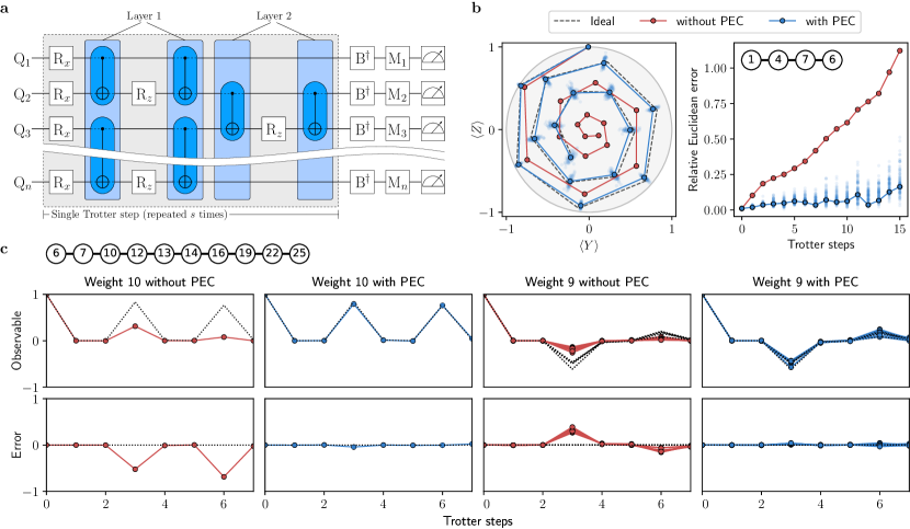
Fig. 3: Error mitigated time evolution of Ising spin chains. (a) Trotter circuit for the Ising Hamiltonian in Eq. (4) over a one-dimensional $n$-qubit lattice. The shaded box represents a single Trotter step and is repeated $s$ times, with associated $R_{X}(2h\delta t)$ and $R_{Z}(-2J\delta t)$ rotations. Each step comprises two instances of two unique cx layers. The $B^{{\dagger}}$ gates select the measurement basis and the $M$ gates facilitate our model-free readout-error mitigation BER2020MTa-arXiv . (b) Time evolution of the Ising model for an $n=4$ spin lattice with and without probabilistic error correction (PEC) for 15 Trotter steps; $h=1$, $J=0.15$, and $\delta t=1/4$. Left: Trotterized time-evolution of the global magnetization ${\mathbf{M}}:=\sum_{n}\left(\left\langle X_{n}\right\rangle,\left\langle Y_{n}\right\rangle,\left\langle Z_{n}\right\rangle\right)/N$ shown in the Y-Z Bloch plane. The experimentally measured evolution (dots and solid lines) is compared to the ideal noise-free one (dashed lines). The bootstrap-estimated error distribution for each data point is shown as clouds (light dots). Right: The error between ideal and measured magnetization vectors, in terms of the relative Euclidean distance $\|{\mathbf{M}}-{\mathbf{M}}_{\mathrm{ideal}}\|_{2}/\|{\mathbf{M}}_{\mathrm{ideal}}\|_{2}$. (c) Time evolution of the Ising model on a one-dimensional ten-qubit lattice sites (top) with $h=1$, $J=0.5236$, and $\delta t=1/4$. All weight-10 (left) and weight-9 Pauli-Z observables (right) are plotted along with the ground truth (dashed).

Probabilistic error cancellation

Once the noise model has been learned, it can be used to mitigate the noise using the PEC method TEM2017BGa . The protocol implements the channel inverse $\Lambda_{i}^{-1}$ through quasi-probabilistic sampling for each of the $l$ layers. The inverse of the map $\Lambda$ is obtained by negating $\mathcal{L}$, leading to a non-physical map given by

$$\Lambda^{-1}(\rho)=\mbox{exp}[-\mathcal{L}](\rho)=\gamma\prod_{k\in\mathcal{K}}\left(w_{k}\cdot-(1-w_{k})P_{k}\cdot P_{k}^{{\dagger}}\right)\rho,$$ (3)

with sampling overhead $\gamma=\exp(\sum_{k\in{\cal K}}2\lambda_{k})$. This amounts exactly to inverting each individual factor in Eq. (1) due to commutativity of the factors. The product structure allows for a direct way of sampling the map. For each $k\in{\mathcal{K}}$ we sample the identity with probability $w_{k}$ or apply the Pauli $P_{k}$ otherwise. We record the number of times $m$ we have applied a non-identity Pauli, compute a final Pauli as the product of all sampled terms. Repeating this for each noise channel $i=1,\ldots,l$ with respective $m_{i}$ and $\gamma_{i}$ values, we construct a circuit instance in which each noisy layer is preceded with the corresponding sampled Pauli. The measurement outcome of the circuit is then multiplied by $\prod_{i=1}^{l}(-1)^{m_{i}}\gamma_{i}$. On average, this implements the inverse maps and produces an unbiased expectation value with sampling overhead $\gamma(l)=\prod_{i=1}^{l}\gamma_{i}$ In Supplementary Materials Sec. SVI.2, we derive an error bound on the final expectation value that considers the errors in all steps of the procedure. The bound states that, given a quantum circuit with $l$ layers whose learning layer satisfies Eq. (2), we can estimate the ideal expectation value $\langle A\rangle$ of an observable $A$ with $\|{A}\|\leq 1$ by the average mitigated estimate $\langle\hat{A}_{N}\rangle$ using $N$ error-mitigated circuit instances, such that

$$|\langle{A}\rangle-\langle\hat{A}_{N}\rangle|\leq(C_{\epsilon}^{l\tau}-1)+\gamma(l)\sqrt{2\log(2/\delta^{\prime})/N}$$

is satisfied with probability at least $1-\delta^{\prime}$. For modest noise, $C_{\epsilon}$ can be expected to be close to one, which leads to a scaling that is only weakly exponential in $l$ and $\tau$. The sampling overhead $\gamma(l)$ dictates the resources needed to obtain a reliable estimator TEM2017BGa .

Quantum simulation of the Ising model

As a practical application for noise mitigation with our proposed noise model we consider time evolution of the one-dimensional transverse-field Ising model due to the Hamiltonian

$$H=-J\sum_{j}Z_{j}Z_{j+1}+h\sum_{j}X_{j}=-JH_{ZZ}+hH_{X},$$ (4)

where $J$ denotes the exchange coupling between neighboring spins and $h$ represents the transverse magnetic field. Unitary time evolution $e^{-iHt}$ can be approximated by a first-order Trotter decomposition $\big{(}e^{iJH_{ZZ}t/s}e^{-ihH_{X}t/s}\big{)}^{s}$ with $s$ segments. We perform the time evolution on a linear chain of qubits, where we implement the unitary $\exp(iJ(Z_{j}Z_{j+1})\delta_{t})$ with $\delta_{t}=t/s$ as a quantum circuit consisting of an $R_{Z}(-2J\delta_{t})$ rotation on qubit $j\!+\!1$ between two cx gates with control and target qubits $j$ and $j\!+\!1$. Similarly, $\exp(-ihH_{x}\delta_{t})$ decomposes into a product of single-qubit rotations $R_{X}(2h\delta_{t})$ on each qubit $j$ (for more details see KIM2021WYMa-arXiv ). This results in circuits of the form shown in Fig. 3a. The circuit contains two unique layers of cx gates, one starting at even and one at odd locations in the qubit chain. Once the noise models for the two layers are learned, we generate random circuit instances. We apply readout-error mitigation on all observables (see BER2020MTa-arXiv for more on readout mitigation). To counter time-dependent fluctuations in the noise we relearn the noise model after fixed intervals (see also Supplementary Materials Sec. SVII). The final observables are obtained after averaging.

As a first experiment, we consider the Ising-model dynamics for a spin chain with four sites with $h=1$ and $J=0.15$. Learning of the first layer was detailed in Fig. 2a–c and resulted in factor $\gamma=1.03$. All other models were learned in a similar fashion. The number of mitigated circuit instances for each $s=1,2,\ldots,15$ is given by $\min(200,40\cdot(\gamma_{1}\gamma_{2})^{2s})$, where $\gamma_{1}$ and $\gamma_{2}$ are the sampling overhead factors for the first and second layer. Each circuit instance is measured 1,024 times.

For each of the $s$ Trotter-steps we compute the global magnetization component $\langle Z\rangle_{s}$ as the overall average of all weight-one Pauli-Z observables, and likewise for $\langle X\rangle_{s}$ and $\langle Y\rangle_{s}$. The resulting $Y$ and $Z$ magnetization components are plotted in Fig. 3b (left) along with the results obtained without PEC and exact simulation. We compare the relative Euclidean distance for the estimated and exact global magnetization in Fig. 3b (right).

Our second experiment considers the simulation of a one-dimensional lattice on ten qubits with $h=1$ and $J=0.5236$ for up to seven Trotter steps. High-weight observables are highly noise sensitive and serve as a demanding test of the method. In Fig. 3c, we compare the results for weight-9 and -10 Pauli-Z observables obtained with and without PEC. Mitigated observables exhibit vanishing residuals.

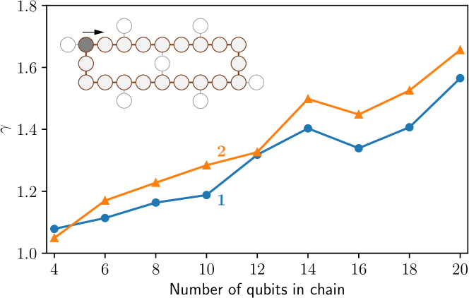
Fig. 4: Mitigation sampling overhead. Sampling overhead $\gamma$ for the two Ising layers as a function of the number of qubits in the Ising lattice chain. The chain is depicted as an inset at the top. The first qubit in the chain is at the top-left (dark shading) and the chain proceeds clockwise (arrow). Layers 1 and 2 have complementary cx gates on alternating pairs of qubits in the chain (see Fig. 3).

Discussion and conclusions

The remarkable accuracy of the error-mitigated observables in Fig. 3 provides strong evidence for the validity of our sparse noise model and learning protocol. It is nonetheless important to discuss potential limitations of our method, such as the sampling overhead. In particular, the variance in the estimator scales with the square of the sampling overhead factor $\gamma(l)$. This factor depends on the number of qubits (see Fig. 4) as well as the circuit depth in terms of the number of layers. We can define a qubit- and depth-normalized version of the scaling factor, $\bar{\gamma}$, which allows us to conveniently express the sampling overhead for $l$ layers on $n$ qubits as $\bar{\gamma}^{nl}$. This normalized parameter itself can also be used as a metric to represent quantum processor performance; improvements in the hardware quality are reflected in lower $\bar{\gamma}$ values, which in turn translate into potentially dramatic decreases in the sampling overhead (see also Supplementary Materials Sec. SVI.3). Our work serves as a powerful example of how classical run-time overheads can be traded for tremendously improved quantum computation on noisy processors. However, this also highlights the importance of improving total circuit execution time wack2021 , which will reduce the practical PEC overhead.

In conclusion, our results demonstrate for the first time a practical path to extend probabilistic error cancellation to remove the noise-induced bias from from high-weight observable across the full circuit (see Fig 3c). This is made possible by our sparse learning protocol, which provides a versatile noise representation with rigorous theoretical bounds and near-constant learning with number of qubits, and an effective noise-inversion scheme. The accuracy of the model-reconstructed noise-fidelity pairs, as shown in Fig 2c, and our error mitigated observables validate the view that the Lindbladian learning is accurate, efficient, and scalable. We expect our learning protocol to be a powerful characterization and benchmarking tool, and more-broadly to enable the study and mitigation of noise in quantum processors at a new scale.

Acknowledgments

The authors thank Sergey Bravyi, Douglas T. McClure, and Jay M. Gambetta for helpful discussions. Research in characterization and noise learning was sponsored in part by the Army Research Office and was accomplished under Grant Number W911NF-21-1-0002. The views and conclusions contained in this document are those of the authors and should not be interpreted as representing the official policies, either expressed or implied, of the Army Research Office or the U.S. Government. The U.S. Government is authorized to reproduce and distribute reprints for Government purposes notwithstanding any copyright notation herein.

Data availability

Data are available from the authors on reasonable request.

Supplementary Information:
Probabilistic error cancellation with sparse Pauli-Lindblad models
on noisy quantum processors

SI Summary of the method

Input: the layer’s qubits and gates, and processor topology
Model definition
• Using the qubit and topology information, define model Paulis $\mathcal{K}$. This set contains all weight-one Paulis supported on the model qubits as well as all weight-two Paulis supported on selected pairs of connected qubits Preparation for model fitting
• Define the measurement bases and determine the fidelities $\mathcal{B}$ needed to fit the model (Section SIV.2.1)
Fidelity estimation
• For each basis, run benchmark circuits at different depths • Fit data with exponentially decaying curves to estimate individual fidelities or fidelity-pair products • Complete the fidelities using unit-depth benchmark circuits or symmetry assumptions • Form vector $\hat{f}$ of estimated fidelities Model fitting
• Form matrix $M=\mathcal{M}(\mathcal{B},\mathcal{K})$ (see Eq. (S12) in Section SIII.3) • Set model parameters to the solution of the following problem (see Eq. (S13) in Section SIII.3) $$\mathop{\mathrm{minimize}}_{\lambda\geq 0}\quad{\textstyle{\frac{1}{2}}}\|M\lambda+\log(\hat{f})/2\|_{2}^{2}$$ Mitigation
• Given a circuit that contains the layer of gates • Generate multiple circuit instances with each layer preceded by a Pauli sampled from the quasi-probability distribution and with a Pauli twirled instance of the layer • Estimate the expectation of the observables of interest and scale by $\gamma$ Note: for layers of two-qubit gates there are two lists of fidelity terms $\mathcal{B}_{1}$ and $\mathcal{B}_{2}$. In this case, we replace $M$ by $\mathcal{M}(\mathcal{B}_{1},\mathcal{K})+\mathcal{M}(\mathcal{B}_{2},\mathcal{K})$. The elements in vector $\hat{f}$ then represents products of two fidelities. See Section SV.1 for more details.

SII Background and review

Most quantum applications combine classical computing with the execution of one or more sets of quantum circuits on the quantum processor. Each circuit execution can roughly be thought of as consisting of three phases: (i) initialization of the quantum processor to the $|{0}\rangle$ ground state; (ii) application of the gates that make up the quantum circuit; and (iii) measurement of the qubits of interest. For each circuit, this process is repeated multiple times to obtain the desired measurement statistics. The process of running a quantum circuit is affected by different sources of noise. The noise associated with the first and last stage is usually combined into so-called state-preparation and measurement (SPAM) error. There are quite a few algorithms for dealing with this type of noise, see for instance BRA2021SKMa ; CHE2020YZFa-arXiv ; BER2020MTa-arXiv for different algorithms and further references. Noise in the second stage consists of global background noise, such as dephasing and decoherence, and noise associated with the application of one or more gates, including cross-talk. Here, we focus on the noise associated with the application of a single operation on one or more qubits. It often helps to write a noisy operation $\tilde{\cal U}$ as a combination of a noise channel $\tilde{\Lambda}$ and the ideal operation ${\cal U}(\rho)=U\rho U^{\dagger}$:

$$\tilde{\cal U}={\cal U}\circ\tilde{\Lambda}.$$

In the remainder of this section we look at techniques for shaping general noise channels $\tilde{\Lambda}$ into more structured and therefore more manageable channels, as well as ways of inverting these new channels.

SII.1 Noise channel simplification

There are many ways to characterize or represent noise channels. Suppose that $\tilde{\Lambda}$ is a noise channel that applies to $n$-qubits and denote by $\{P_{i}\}_{i=0}^{4^{n}-1}$ the Pauli basis for the corresponding Hilbert space. Then we can express $\tilde{\Lambda}$ in terms of the Pauli transfer matrix $\mathcal{T}_{\tilde{\Lambda}}$ with entries

$$T_{\tilde{\Lambda}}[a,b]=\frac{1}{2^{n}}\mathrm{Tr}\left[P_{a}^{{\dagger}}(\tilde{\Lambda}(P_{b}))\right].$$

In general, this will be a dense matrix, and working with the explicit form with $\mathcal{O}(4^{2n})$ nonzero coefficients therefore quickly becomes intractable, certainly because all coefficients need to be estimated in tomography. However, it has been shown knill2004fault ; kern2005quantum ; geller2013efficient ; wallman2016noise that conjugation of the noise channel with randomly sampled operators from the Pauli group results in an averaged channel

$$\Lambda(\cdot)=\mathbb{E}_{i}\big{[}P_{i}^{{\dagger}}\tilde{\Lambda}(P_{i}^{\dagger}\cdot P_{i})P_{i}^{\dagger}\big{]},$$ (S1)

with a diagonal transfer matrix $T_{\Lambda}[a,b]=\delta_{a,b}T_{\tilde{\Lambda}}[a,b]$. The averaging operation in (S1) is called a Pauli twirl. In addition to a much more compact representation, this transfer matrix is also easily inverted. The quantities on the diagonal of the transfer matrix represent the Pauli fidelities $f_{a}=2^{-n}\mathrm{Tr}\left[P_{a}(\tilde{\Lambda}(P_{a}))\right]$. We can use the symplectic Walsh-Hadamard transformation to convert these fidelities FLA2020Wa to coefficients

$$c_{b}=\frac{1}{2^{n}}\sum_{a}(-1)^{\langle a,b\rangle_{sp}}f_{a},$$ (S2)

where $\langle a,b\rangle_{sp}$ denotes the symplectic inner product of Paulis $P_{a}$ and $P_{b}$, which is zero if the Paulis commute (that is $[P_{a},P_{b}]=P_{a}P_{b}-P_{b}P_{a}=0$), and one otherwise. These coefficients allow us to then rewrite the noise operator applied to the density matrix $\rho$ as a Pauli channel:

$$\Lambda(\rho)=\sum_{i}c_{i}P_{i}\rho P_{i}^{{\dagger}},$$ (S3)

where the vector $c=[c_{i}]$ of all coefficients represents a distribution: $c_{i}\geq 0$ and $\sum_{i}c_{i}=1$. The Pauli twirl can be approximated by generating multiple instances of the appropriate quantum circuit, each with a Pauli term $P_{a}$ sampled uniformly at random from the $n$-Pauli matrices. This may seem difficult, since, in general, we are not given an isolated noise channel but rather have access only to a noisy gate $\tilde{\cal U}={\cal U}\circ\tilde{\Lambda}$. In this case we just want to twirl $\tilde{\Lambda}$, which is possible by pushing the Pauli through the $U$ gate, when this is a Clifford gate knill2004fault ; kern2005quantum ; geller2013efficient ; wallman2016noise . To see how this works, observe that

$$UP_{a}^{{\dagger}}\tilde{\Lambda}(P_{a}\cdot P_{a}^{{\dagger}})P_{a}U^{\dagger}=UP_{a}^{{\dagger}}(U^{{\dagger}}U)\tilde{\Lambda}(P_{a}\cdot P_{a}^{{\dagger}})(U^{{\dagger}}U)P_{a}U^{\dagger}=P_{a^{U}}\;\tilde{\cal U}(P_{a}\cdot P_{a}^{{\dagger}})P_{a^{U}}^{\dagger}.$$

When $U$ is a Clifford operator, it is well known that the conjugation of one Pauli operator results in another Pauli, namely $UP_{a}U^{{\dagger}}=P_{a^{U}}$. That means that Pauli twirling for Clifford operators $U$ can be conveniently implemented by sampling a random $P_{a}$ term and applying this terms and its conjugate under $U$ to the circuit, around the noisy gate to get $P_{a^{U}}\tilde{U}P_{a}$. Pauli operators themselves are formed as the direct product of Pauli matrices $X$, $Y$, and $Z$ and the two-by-two identity matrix, and $n$-Paulis can therefore be efficiently represented by a string $\{I,X,Y,Z\}^{n}$ of length $n$, or in symplectic form as a binary vector of length $2n$. The latter representation enables a computationally efficient way of conjugating the Pauli operator by any Clifford operator AAR2004Ga , and therefore allows us to efficiently find $P_{a^{U}}$ for a given $P_{a}$. Since Pauli operators can be implemented using single-qubit gates, we can often simplify the circuits of twirled gates. Any single-qubit directly preceding or following the gate can be combined with the respective single-qubit gate of operators $P_{a}$ or $P_{a^{U}}$. This can reduce or even completely eliminate the circuit overhead of the Pauli twirl.

Twirling is possible over groups wallman2016noise ; cai2019constructing other than the Pauli group. In general, given a group $\mathcal{G}$, we can define the twirled noise channel

$$\Lambda_{\mathcal{G}}:=\frac{1}{|\mathcal{G}|}\sum_{G\in\mathcal{G}}G^{-1}\circ\tilde{\Lambda}\circ G.$$

When $\mathcal{G}$ is the Clifford group, or any other two-design, the resulting transfer matrix $T_{\Lambda_{\mathcal{G}}}$ is not only diagonal, but such that the fidelities for Pauli operators other than the identity (which is always one) are all equal. This means that the new twirled noise channel can be described by only a single parameter. In case both $U$ and $G$ are elements of the Clifford group, it holds that the conjugated operator $UGU^{{\dagger}}$ remains an element of the Clifford group. As in the Pauli case, one can efficiently represent elements from the Clifford group and compute the conjugation. However, the problem is that the circuit implementation of a Clifford gate can have a significant depth BRA2020Ma , and may therefore introduce an unacceptable amount of noise itself.

SII.2 Quasi-probabilistic noise inversion

The probabilistic error cancellation method as given in TEM2017BGa ; END2018BLa asks that for the general procedure an ideal ${\cal U}$ operation is expanded into a set of noisy operators $\{\tilde{\cal U}_{i}\}_{i}$ that can be implemented on the quantum hardware. However, we are in the particular situation that our noisy operations for each layer are exactly of the form $\tilde{\cal U}={\cal U}\circ\Lambda$, where $\Lambda$ is a Pauli channel. In particular, as explained in the previous section, the general procedure considered in TEM2017BGa ; END2018BLa can be reduced to this special case after Pauli twirls have been applied. We are then in the setting where it is sufficient to only focus on the noise of the Pauli noise channel $\Lambda$ and implement its inverse $\Lambda^{-1}$ in experiment.

When represented as the diagonal Pauli transfer matrix $T_{\Lambda}$ it is clear that the inverse should have a Pauli transfer matrix given by $T_{\Lambda}^{-1}=\mbox{diag}(f_{a}^{-1})$. That is, a diagonal matrix with the inverse fidelities on the diagonal. If then follows from the Walsh-Hadamard transform in (S2), that we would like to have a Pauli channel with coefficients

$$c_{b}^{\mathrm{inv}}=\frac{1}{2^{n}}\sum_{a}(-1)^{\langle a,b\rangle_{sp}}\frac{1}{f_{a}}.$$

However, except for the case where all fidelities are one, the resulting coefficients will contain negative values, and therefore does not represent a physical Pauli channel. The method proposed in TEM2017BGa addresses this as follows. We can first rewrite the desired channel as

$$\sum_{i}c_{i}^{\mathrm{inv}}P_{i}\rho P_{i}^{{\dagger}}=\sum_{i}\mathrm{sgn}(c_{i}^{\mathrm{inv}})|c_{i}^{\mathrm{inv}}|P_{i}\rho P_{i}^{{\dagger}}=\gamma\sum_{i}\mathrm{sgn}(c_{i}^{\mathrm{inv}})\gamma^{-1}|c_{i}^{\mathrm{inv}}|P_{i}\rho P_{i}^{{\dagger}}\;,$$

where $\mathrm{sgn}$ denotes the signum function and $\gamma:=\sum_{i}|c_{i}^{\mathrm{inv}}|$. The transformed coefficients $\hat{c}_{i}^{\mathrm{inv}}=\gamma^{-1}|c_{i}^{\mathrm{inv}}|$ are clearly nonnegative and by definition of $\gamma$, sum up to one, and therefore represent a distribution. In order to implement noise inversion the algorithm proceeds as follows. First, a random Pauli $a$ is sampled according to the distribution $\hat{c}_{i}^{\mathrm{inv}}$. We store the sign $\mathrm{sgn}(c_{a}^{\mathrm{inv}})$ and form a circuit with that includes the sampled $P_{a}$ prior to the noise channel. We then estimate the expectation values of any desirable observable and scale it by the sign as well as by $\gamma$. When computed over multiple random samples $P_{a}$, the empirical mean value of the scaled observables then provide an unbiased estimator of the ideal expectation value that would result from a noiseless circuit. The cost of sampling from the quasi-probabilistic distribution is an increase in variance in the expected value by a factor of $\mathcal{O}(\gamma^{2})$.

SII.3 Scalable noise models

While working with explicit Pauli channels is convenient, they do require the storage and processing of $4^{n}$ coefficients for $n$ qubits in general. In order to reduce the model complexity and maintain efficiency, the work presented in FLA2020Wa considers Pauli channels with bounded degree correlations. The probability distribution representing the Pauli channel in this case is factored based on the individual terms and such that certain terms are conditionally independent. The resulting probabilities are in Gibbs form and can be reconstructed from locally measured patches at the expense of computing the full partition function of the distribution. While the resulting structure can help reduce the noise channel representation, application of the model to noise mitigation and computing or sampling from the noise inverse remains challenging. We therefore focus on a Pauli model that retains the local correlation but is better suited to the probabilistic error-cancellation protocol.

SIII Pauli-Lindblad noise model

We propose the use of a locally correlated noise model that is motivated by the continuous-time Markovian dynamics of open quantum systems. These dynamics can be described by a quantum master equation. When appropriately rewritten in diagonal form, this can be expressed as the Lindblad equation BRE2002Pa $\frac{d}{dt}\rho(t)=\mathcal{L}\rho(t)$, where $\mathcal{L}(\rho)=-i[H,\rho]+\sum_{k}\left(A_{k}\rho A_{k}^{{\dagger}}-\frac{1}{2}A_{k}^{{\dagger}}A_{k}\rho-\frac{1}{2}\rho A_{k}^{{\dagger}}A_{k}\right)$. For a general Lindbladian, the unitary part of the dynamics is described by the Hamiltonian $H$, and $A_{k}$ are the Lindblad operators. The resulting channel after evolution time $t$ is then the formal exponential $T_{t}=\mbox{exp}\left[{\cal L}t\right]$.

The Pauli-Lindblad noise model we consider contains no internal Hamiltonian dynamics and we therefore do not consider a Hamiltonian contribution. We want to generate a Pauli channel and therefore take $A_{k}=\sqrt{\lambda_{k}}P_{k}$ for a set of Pauli operators $\{P_{k}\}_{k\in{\cal K}}$ we enumerate with an index set ${\cal K}$:

$$\mathcal{L}(\rho)=\sum_{k\in{\cal K}}\lambda_{k}\left(P_{k}\rho P_{k}-\rho\right).$$ (S4)

In particular we assume that $|{\cal K}|\ll 4^{n}-1$ is a set that is only of polynomial size in the number of qubits. This means the model is determined by a set of non-negative numbers $\lambda_{k}\geq 0$ for $k\in{\cal K}$. We will discuss the choice of this set for our experimentally considered set up in section SIII.2. In general, the set can be chosen as to account for the correlations that are present in the quantum hardware of interest. Since we are only interested in a particular noise model, we set the dynamics to be at time $t=1$ and directly define the sparse Pauli-noise model as $\Lambda=\mbox{exp}\left[{\cal L}\right]$.

When working in the matrix representation expressing the Lindbladian $\mathcal{L}$, which we denote by $\mbox{vec}\left[\mathcal{L}\right]$, it follows that the sparse noise model $\Lambda$ is given by the conventional matrix exponential

$$\mbox{vec}\left[\Lambda\right]=e^{\mbox{vec}\left[\mathcal{L}\right]}.$$ (S5)

Here, the matrix representation of the Lindbladian is defined as

$$\mbox{vec}\left[\mathcal{L}\right]=\sum_{k\in{\cal K}}\lambda_{k}\left(P_{k}\otimes P_{k}^{T}-I\otimes I\right).$$ (S6)

Note that for any two Pauli operators $P$ and $Q$ it holds that

$$(P\otimes P^{T})(Q\otimes Q^{T})=(PQ\otimes(QP)^{T})=((\pm PQ)\otimes(\pm(PQ)^{T})=(QP\otimes(PQ)^{T})=(Q\otimes Q^{T})(P\otimes P^{T}).$$

This shows that the terms in (S6) commute, and also expresses the fact that Pauli channels commute. Given the commutativity of the terms, we can write the time-evolution operator as

$$\mbox{vec}\left[\Lambda\right]=\prod_{k}e^{-\lambda_{k}}e^{\lambda_{k}P_{k}\otimes P_{k}^{T}}$$ (S7)

Exponentiation with a Pauli operator can we written as

$$e^{\lambda(P\otimes P^{T})} =\cosh(\lambda)(I\otimes I)+\sinh(\lambda)(P\otimes P^{T})$$

$$=\frac{e^{\lambda}+e^{-\lambda}}{2}(I\otimes I)+\frac{e^{\lambda}-e^{-\lambda}}{2}(P\otimes P^{T})$$ (S8)

Combining (S7) and (S8) and we obtain the final form of the noise model as

$$\Lambda(\rho)=\prod_{k}\left(w_{k}\cdot+(1-w_{k})P_{k}\cdot P_{k}^{{\dagger}}\right)\rho,$$ (S9)

where $w_{k}=(1+e^{-2\lambda_{k}})/2$. Given the time evolution of states in (S9), it is natural to ask what effect it has on Pauli operators. The fidelity $f_{a}$ of a Pauli operator $P_{a}$ can be expressed as

$$f_{a} =\frac{1}{2^{n}}\mathrm{Tr}\left[P_{a}^{{\dagger}}\Lambda(P_{a})\right]=\frac{1}{2^{n}}\mathrm{Tr}\Big{[}P_{a}^{{\dagger}}P_{a}\prod_{\{a,k\}=0}(2w_{k}-1)\Big{]}$$

$$=\prod_{\langle a,k\rangle_{sp}=1}(2w_{k}-1)=\prod_{\langle a,k\rangle_{sp}=1}e^{-2\lambda_{k}}=\exp\left(-2\sum_{k\in\mathcal{K}}\lambda_{k}\langle a,k\rangle_{sp}\right).$$ (S10)

We can define a matrix $M$ with entries $M_{a,b}=\langle a,b\rangle_{sp}$, such that $M_{a,b}=0$ if Paulis $P_{a}$ and $P_{b}$ commute, and $M_{a,b}=1$ otherwise. Denoting by $f$ and $\lambda$ the full vector of Pauli fidelities and model coefficients, respectively, we can compactly express (S10) as

$$-\log(f)/2=M\lambda\;,$$ (S11)

where the logarithm is applied elementwise. Finally, we observe that the coefficients $w_{k}$ in (S9) are all nonnegative, and that the fidelity for the identity operator is always one, since all Pauli terms commute with the identity. It follows that (S9) is a valid Pauli channel for all $\lambda\geq 0$.

SIII.1 Channel operations

The Lindbladian noise channel in (S9) has some useful properties. First, changing the evolution time amounts to scaling $\lambda$. Second, given two separate noise channels with parameters $\lambda_{1}$ and $\lambda_{2}$, it follows from multiplicativity of fidelities under successive Pauli channels that

$$-\log(f_{1}f_{2})/2=-\log(f_{1})/2-\log(f_{2})/2=M\lambda_{1}+M\lambda_{2}=M(\lambda_{1}+\lambda_{2})\;,$$

which shows that combination of channels amounts to addition of the coefficients. The inverse of a channel is characterized by inverse fidelities, and it directly follows from

$$-\log(1/f)/2=\log(f)/2=-M\lambda=M(-\lambda)$$

that the inverse noise model is obtained by simply negating the coefficients.

SIII.2 Sparse models

Quantum circuits are generally transpiled into native single- and two-qubit gates applied to individual qubits or pairs of qubits that are topologically connected, that is, neighboring qubits. The noise associated with the application of these gates can be expected to have limited range and therefore be negligible beyond some local neighborhood around the qubits to which the operation is applied. This suggests it may not be necessary to include all possible Pauli terms in (S9), and motivates us to simplify the model and include only a select subset of Pauli terms $P_{k}$. For instance, we could include those Paulis that contain only a single non-identity term, or two such terms on neighboring qubits. Such sparse models can be represented far more efficiently than their full counterpart. For a linear topology of $n$ qubits, the number of coefficients $\lambda$ reduces from $4^{n}-1$ to a mere $3n+9(n-1)$, which is clearly far more scalable in terms of the number of qubits.

SIII.3 Learning the model

In order to characterize a noise channel we need to find model coefficients that best explain the experimental data. For the proposed noise model, a practical way of determining the model coefficients follows directly from equation (S11). We first form a vector $f$ of fidelity for Pauli terms in some list $B$. Given model Paulis $K$ we can form the matrix

$$M=\mathcal{M}(B,K)\quad\mbox{such that}\quad M_{i,j}=\begin{cases}0&[B_{i},K_{j}]=0\\ 1&[B_{i},K_{j}]\neq 0.\end{cases}$$ (S12)

We then find nonnegative coefficients $\lambda$ such that $M\lambda$ is as close to $-\log(f)$ as possible. When measuring in Euclidean distance (other norms could be used here as well), this can be conveniently formulated as a nonnegative least-squares problem:

$$\lambda(f):=\mathop{\mathrm{argmin}}_{\lambda\geq 0}\quad{\textstyle\frac{1}{2}}\|M\lambda+\log(f)/2\|_{2}^{2}\;.$$ (S13)

The columns in matrix $M$ correspond to the Pauli terms included in the model, denoted by $\mathcal{K}$, whereas the rows could be any of the $4^{n}$ Pauli operators, although we generally omit the row for the identity operator since all its entries as well as the log fidelity are zero. In case of the sparse noise model described in Section SIII.2, the number of model Paulis is relatively small and matrix $M$ will have far more rows than columns. The model coefficients are well defined if the solution of (S13) is unique, which is guaranteed whenever $M(\mathcal{B},\mathcal{K})$ has full column rank.

SIII.4 Variance in mitigated observable

We now consider the variance in the error-mitigated observable. Starting with binomial distribution with $p(1)=p$ and $p(0)=q=1-p$ and $n$ trials we have mean $np$ and variance $npq$. For the estimation of observables we sample from $\pm 1$ which means scaling by two and subtracting one per trial, which gives mean $2np-n$ and variance $2^{2}npq$. In order to obtain the observable we divide by the number of trials and scale by $\gamma$, which leads to an updated mean of $2p\gamma-\gamma=(2p-1)\gamma$ and variance $(\gamma/n)^{2}(4npq)=(4\gamma^{2}/n)pq$. The ideal observable or fidelity $f$ is equal to the mean, namely $(2p-1)\gamma=f$. Rewriting gives

$$p=\frac{1}{2}\left(\frac{f}{\gamma}+1\right),\qquad q=1-p=\frac{1}{2}\left(1-\frac{f}{\gamma}\right),\qquad pq=\frac{1}{4}\left(1-\frac{f^{2}}{\gamma^{2}}\right).$$

Using this we obtain variance

$$\frac{4\gamma^{2}}{n}pq=\frac{1}{n}\left(\gamma^{2}-f^{2}\right).$$

In order to keep the variance of the estimator fixed we therefore need to scale $n$ proportional to $\gamma^{2}$.

SIV Noise learning for single-qubit gates with crosstalk

The proposed noise model readily applies to benchmarking and mitigating the noise in layers of single-qubit gates. A common assumption in this setting is that, for a given qubit, the noise is independent of the gate that is applied. Here we refine this and assume that the noise channel associated with a layer of single-qubit operations depends only on the particular subset of qubits that contain a gate. The motivation for this is that application of a gate to a qubit can result in crosstalk, which depends in part on qubit connectivity as well as the presence or absence of gates on neighboring qubits.

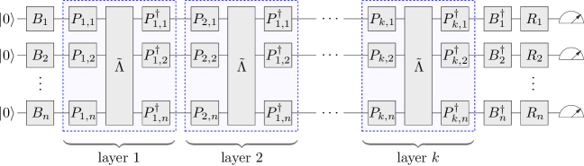
Fig. S1: Benchmark circuit.

The estimation of the fidelities that will be needed to reconstruct the sparse noise model uses a slightly simplified version of the algorithm proposed in FLA2020Wa and considers the setting where gates are applied to all qubits. The benchmark circuits are of the form shown in Figure S1, where the single-qubit gates shown are all noiseless. Although this may seems to contradict the assumption that we only have access to noisy gates, note that the noise is assumed to be independent of the unitaries applied to each qubit, which therefore allows us to apply as many consecutive unitaries as we like with only a single noise term by simply multiplying the individual unitaries into a single final unitary and applying the noisy version of this final unitary. That means that successive gates $B_{1}$ and $P_{1,1}$ will be combined into some unitary $U_{1}$, which is then applied to the circuit along with the associated noise channel. For convenience we assume that the noise following the $R_{i}$ gates appears as readout errors. Having convinced ourselves that we can actually implement the circuits from Figure S1, we now describe the different components. Gates $B_{i}$ and $B_{i}^{{\dagger}}$ implement basis changes between different Pauli bases. Each cycle consists of the noise channel $\hat{\Lambda}$ conjugated by random Pauli terms $P_{i,j}$. When averaged over all possible Pauli terms, this implements a Pauli twirl of the noise channel $\tilde{\Lambda}$, resulting in a Pauli channel $\Lambda$, which has a diagonal Pauli-transfer matrix with fidelity $f_{i}$ for Pauli $P_{i}$. The final gates $R_{i}$ are sampled uniformly at random from $\{I,X\}$ and are used in combination with classical post-processing to diagonalize the readout error CHE2020YZFa-arXiv ; BER2020MTa-arXiv . In order to determine the fidelity $f_{i}$ we start with the Pauli-Z term $P_{z(i)}$ that has the same support as $P_{i}$. The initial state $\tilde{\rho}$ is a noisy version of $|{0}\rangle\langle{0}|$ with associated state-preparation fidelity $s_{i}=\mathrm{Tr}[P_{z(i)}\tilde{\rho}]$. The basis change gates $B_{i}$ change $P_{z(i)}$ to $P_{i}$, and we then apply $k$ cycles, each contributing a fidelity term $f_{i}$. As a result of diagonalization of the readout errors, we can define a readout fidelity $r_{i}=r_{z(i)}$. Overall, this means that the expected value for the observable $P_{i}$, measured through observable $P_{z(i)}$ using bases changes, is given by $(s_{i}r_{i})f_{i}^{k}=\alpha_{i}f_{i}^{k}$. Dividing the estimates obtained for $k$ and zero cycles, then gives an unbiased estimate of $f^{k}$, free of state-preparation and readout errors.

Now that we have access to estimates of individual fidelities of $\Lambda$, we would like to fit a model that can capture crosstalk. For this we propose to use a two-local Lindblad model, with coefficients terms $\mathcal{K}$ given by the union of all unit-weight Paulis and all weight-two Paulis whose support corresponds to connected qubits. Given these coefficients we need to determine the set $\mathcal{B}$ of Paulis for which we estimate the fidelity, such that the matrix $M(\mathcal{B},\mathcal{K})$ is full rank. For this we use the result from Section SIV.1, which shows that choosing $\mathcal{B}=\mathcal{K}$ results in a square invertible $M$. With this, the next step is to estimate the fidelities and fit the model. This is where sampling error comes in: we can only estimate $\alpha_{i}f_{i}^{k}$ up to an additive error $\epsilon$ that decreases with the number of circuit instances. In Section SIV.2 we therefore study the sample complexity and the final accuracy of the noise model and its inverse. For a given circuit it is generally possible to estimate a number of fidelities. In section SIV.2.1 we show, under mild conditions on the qubit topology, that it suffices to measure in nine different bases.

SIV.1 Fidelities for model fitting

We can represent qubit topology as an undirected graph in which each vertex corresponds to a qubit, and where edges indicate a physical or logical connection between qubits. For our two-local Lindbladian noise model we choose model coefficients $\mathcal{K}$ corresponding to Paulis with support on qubits that are connected by edges, as well as all Paulis that are supported on subsets of the former supports, which in this case corresponds to the individual qubits. A direct consequence of the result below is that $\mathcal{M}(\mathcal{K},\mathcal{K})$ is full rank. Choosing any set of benchmark fidelities $\mathcal{B}$ that includes $\mathcal{K}$ gives a full column-rank $M$ and thus ensures that the least-squares problem has a unique solution.

Theorem SIV.1.

Given a set $\{\mathcal{S}_{i}\}$ of supports $\mathcal{S}_{i}\subseteq[n]$. Define the set $\mathcal{V}=\{\mathcal{V}_{j}\}$ as the union over $i$ of all non-empty subsets of $\mathcal{S}_{i}$, including the sets themselves. For each $j$ let $\mathcal{P}_{j}$ be the set of all $n$-qubit Pauli strings supported on $\mathcal{V}_{j}$, and let $\mathcal{P}=\bigcup_{j}\mathcal{P}_{j}$. Then $M(\mathcal{P},\mathcal{P})$ is full rank.

Proof.

Since permuting the matrix rows and columns leaves the rank unchanged we assume that the sets $\mathcal{V}_{j}$ are ordered according to increasing cardinality and that the Pauli strings in each set $\mathcal{P}_{j}$ are sorted lexicographically. Define $V=-2M(\mathcal{P},\mathcal{P})$ and partition the matrix into blocks such that block $V(i,j)=-2M(\mathcal{P}_{i},\mathcal{P}_{j})$. These blocks are concisely expressed as $V(i,j)=O(i,j,S)-O(i,j,\mathbb{1})$, where $\mathbb{1}$ is a $3$-by-$3$ matrix of ones, and

$$O(i,j,op)=\bigotimes_{\ell=1}^{n}\begin{cases}op&\ell\in\mathcal{V}_{i}\cap\mathcal{V}_{j}\\ \mathbf{e}&\ell\in\mathcal{V}_{i}\setminus\mathcal{V}_{j}\\ \mathbf{e}^{T}&\ell\in\mathcal{V}_{j}\setminus\mathcal{V}_{i}\\ 1&\ell\not\in\mathcal{V}_{j}\cup\mathcal{V}_{j}\end{cases},\qquad S=\left(\begin{array}[]{rrr}1&-1&-1\\ -1&1&-1\\ -1&-1&1\end{array}\right),$$ (S14)

and $\bf{e}$ denotes a column vector of ones of length three with transpose $\bf{e}^{T}$. Note that matrices $S$ and $Q:=S-\mathbb{1}$ are invertible. We prove invertibility of $V$ by reducing it to a block-diagonal matrix with invertible block by iteratively applying sweep operations. Sweeping of the blocks in row $i$ or column $j$ by those $k$ is done only when $\mathcal{V}_{k}\subset\mathcal{V}_{i}$ or $\mathcal{V}_{k}\subset\mathcal{V}_{j}$, respectively. The sweep operations are defined as

$$\begin{split}\mbox{row\_sweep$(i,k$):}\ \ &V(i,j)\leftarrow V(i,j)-O(i,k,I)V(k,j),\\ \mbox{column\_sweep($j,k)$:}\ \ &V(i,j)\leftarrow V(i,j)-V(i,k)O(k,j,I).\end{split}$$ (S15)

The structure of $O(i,j,op)$ in terms of the locations of matrices and additional terms $\bf{e}$, $\bf{e}^{T}$, and $1$ is prescribed by the sets $\mathcal{V}_{i}$ and $\mathcal{V}_{j}$, and we now show that $V(i,j)$ can always be written as a sum of tensors sharing the same structure. This is immediate for the initial $V(i,j)$ and we therefore focus on the updates in (S15). For the row update we consider the term $O(i,k,I)V(k,j)$, or, since we are only interested in structure, $O(i,k,I)O(k,j,op)$. By writing out a table of terms based on membership of $\ell$ in $\mathcal{V}_{i}$, $\mathcal{V}_{j}$, and $\mathcal{V}_{k}$, with the constraint that $\mathcal{V}_{k}\subset\mathcal{V}_{i}$, it can easily be verified that this indeed holds. Of special interest is the case where $\ell\in\mathcal{V}_{i,j}$ and $\ell\not\in\mathcal{V}_{k}$. In this case the $\ell$th terms in $O(i,k,I)$ and $O(k,j,op)$ are $\bf{e}$ and $\bf{e}^{T}$ respectively, which means that their product is the matrix $\mathbb{1}$. The same approach shows that column sweeps also maintain the structure. For convenience we represent by $B^{(\ell)}(i,j)$ the value of block $V(i,j)$ at iteration $\ell$ as a sum of matrix products of $w_{i,j}$ matrices, thus omitting the fixed non-matrix terms in the full representation. As seen above, the initial block values are given by $B^{(0)}(i,j)=S^{\otimes w_{i,j}}-\mathbb{1}^{\otimes w_{i}}$, where we define $A^{\otimes 0}=1$. We provide a sweeping algorithm such that

$$B^{(\ell)}(i,j)=\begin{cases}Q^{\otimes w_{i,j}}&\mbox{if $i=j$ and $w_{i,j}\leq\ell$},\\ 0&\mbox{if $i\neq j$ and $w_{i,j}\leq\ell$},\\ Q^{\otimes w_{i,j}}&\mbox{if $w_{i,j}=\ell+1$},\\ S^{\otimes w_{i,j}}-\mathcal{Q}(w_{i,j},\ell)&\mbox{if $w_{i,j}>\ell+1$},\end{cases}$$ (S16)

holds for all $\ell\geq 0$, where $\mathcal{Q}(w,\ell)$ is the sum of matrices $\{\mathbb{1},Q\}^{\otimes w}$ that contain at most $\ell$ terms equal to $Q$. The expressions for the second and third case of (S16) are special cases of $S^{\otimes w_{i,j}}-\mathcal{Q}(w_{i,j},\ell)$. Namely, we have $S^{\otimes w}=(\mathbb{1}+Q)^{\otimes w}=\mathcal{Q}(w,w)$, while for $w\geq 1$ it holds that $\mathcal{Q}(w,w)-\mathcal{Q}(w,w-1)=Q^{\otimes w}$, and therefore

$$S^{\otimes w}-\mathcal{Q}(w,w-1)=Q^{\otimes w}\quad\mbox{and}\quad S^{\otimes w}-\mathcal{Q}(w,\ell\geq w)=0.$$

It can be verified that (S16) holds for $\ell=0$ by observing that $\mathcal{Q}(w,0)=\mathbb{1}^{\otimes w}$. Assume that (S16) holds for some $\ell\geq 0$. Then the blocks can be arranged as shown in Figure S2. Because $w_{i,j}=w_{j,i}\leq w_{i}$ we can ignore all rows $i$ with $w_{i}\leq\ell$, and likewise for the columns, since $B^{(\ell)}(i,j)=B^{(\ell)}(j,i)^{T}$. Submatrix A consists of all blocks $(i,j)$ with $w_{i}\!=\!w_{j}\!=\!\ell+1$, and it follows from $w_{i,i}=w_{i}$ for the diagonal blocks and $w_{i,j}<w_{i}$ for the off-diagonal blocks that A is block diagonal with $B^{(\ell)}(i,i)=Q^{\otimes\ell+1}$. Submatrix B satisfies $w_{j}=\ell+1$ and $w_{i}>\ell+1$ and therefore also has blocks with weight at most $\ell+1$. This means that the blocks are again either $Q^{\otimes\ell+1}$ or zero, and likewise for submatrix C. Given this structure it is easily seen that we can clear block $B$ by sweeping rows $i\in\mathcal{I}=\{i\mid w_{i}>\ell+1\}$ with rows $k\in\mathcal{K}=\{k\mid w_{k}=\ell+1\}$. Consider an arbitrary row $i\in\mathcal{I}$. For each $k\in\mathcal{K}$ we have $|\mathcal{V}_{k}|=\ell+1$, and it therefore follows from $|\mathcal{V}_{i}|=w_{i}$ and the assumption that all non-empty subsets of $\mathcal{V}_{i}$ are present, that there are exactly $\binom{w_{i}}{\ell+1}$ elements $k\in\mathcal{K}$ for which $\mathcal{V}_{k}\subset\mathcal{V}_{i}$ and $w_{i,k}=\ell+1$. We therefore need to sweep row $i$ with precisely these $k$ values, which we denote by $\mathcal{K}^{\prime}$ with implicit dependency on $i$ and $\ell$. For the effect on block D, consider a block $(i,j)$ with an arbitrary $j$ for which $w_{j}>\ell+1$. If $w_{i,j}\leq\ell$ we have $B^{(\ell)}(i,j)=0$ and it follows from $\mathcal{V}_{k}\subset\mathcal{V}_{i}$ that $w_{k,j}\leq\ell$ for all $k\in\mathcal{K}^{\prime}$, which means that all updates to it are zero as well. For block $B^{(\ell)}(i,k)$ in C to be nonzero we must have $\mathcal{V}_{k}\subset\mathcal{V}_{j}$, which is the case for exactly $\binom{w_{i,j}}{\ell+1}$ values of $k\in\mathcal{K}^{\prime}$ since $|\mathcal{V}_{i}\cap\mathcal{V}_{j}|=w_{i,j}$. All elements $k$ outside this set, say $\mathcal{K}^{\prime\prime}$, will have $|\mathcal{V}_{j}\cap\mathcal{V}_{k}|<w_{i}=\ell+1$ and therefore correspond to a zero block $(k,j)$. Because each block $(k,j)$ for $k\in\mathcal{K}^{\prime\prime}$ is equal to $Q^{\otimes\ell+1}$ and multiplied by $O(i,j,I)$, we conclude that block $(i,j)$ is swept by all matrices $\{\mathbb{1},Q\}^{\otimes w_{i,j}}$ with exactly $\ell+1$ terms equal to $Q$. That means that $B^{(\ell+1)}(i,j)$ is updated to $S^{\otimes w_{i,j}}-\mathcal{Q}(w_{i,j},\ell+1)$. Once submatrix B is cleared we can repeat the same set of sweeps over the column indices. Since all blocks in B are zero this does not affect submatrix D and only zeros out all blocks in C. The claim that (S16) holds for all $\ell\geq 0$ then follows directly by induction. For $\ell=\max_{i}(w_{i})$ we see that the diagonal elements $B^{(\ell)}(i,i)$ are $Q^{\otimes w_{i}}$ and invertible, and all off-diagonal elements are zero, as required.

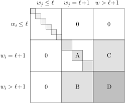
Fig. S2: Structure of the blocks $B^{(\ell)}(i,j)$ at iteration $\ell$.

∎

SIV.2 Sample complexity and error analysis

In order to fit the Lindbladian noise model we need to estimate individual fidelities $f_{i}$. We refer to the set of Paulis that are measured in the experiment as $\mathcal{B}$. The task at hand is to reconstruct the full Pauli-Lindblad model $\Lambda$ by only measuring a sparse subset $|\mathcal{B}|\ll 4^{n}-1$ of fidelities and then fitting the model to determine the parameters $\lambda_{k}$ with $k\in\mathcal{K}$. The deviation of these parameters from the assumed ground truth is bounded in (S20). The error bound in the following theorem SIV.2 bounds the deviation of all fidelities of the ground truth Pauli-Lindblad model $\Lambda$ from the model fidelities obtained parameter estimates for $\lambda_{k}$. The estimation of the directly measured fidelities from $\mathcal{B}$ is done using random circuit instances of the form shown in Figure S1 for various cycle lengths $k$. For a fixed $k$, the expected value for observable $P_{i}\in\mathcal{B}$, measured using appropriate basis changes and readout twirling, is given by $\alpha_{i}f_{i}^{k}$. Measuring a single shot for each qubit for a single circuit instance is equivalent to sampling an element from a distribution over $\{-1,1\}$ with expectation value $\alpha_{i}f_{i}^{k}$. For the deviation from the expected value we can apply Hoeffding’s inequality, which states that for given $N$ independent random variables $X_{j}$ sampled from any distribution $[-\beta,\beta]$, the deviation of $\bar{X}=N^{-1}\sum_{i=1}^{N}X_{i}$ to the expected value satisfies

$$\Pr\left(\big{|}\bar{X}-\mathbb{E}(X)\big{|}\geq\epsilon\right)\leq 2\exp\left(-\frac{N\epsilon^{2}}{2\beta}\right).$$ (S17)

From this it follows that, by taking $N\geq 2\log(2/\delta)/\epsilon^{2}$ samples, the estimate $\alpha_{i}f_{i}^{k}+\epsilon_{i,k}$ satisfies $|\epsilon_{i,k}|\leq\epsilon$ with probability at least $1-\delta$. The number of samples in this case corresponds to the number of circuit instances. We will revisit the sample complexity below, but first state the following result assuming sufficiently accurate samples:

Theorem SIV.2.

Denote the Pauli terms in a given Pauli-Lindblad channel by $\mathcal{K}$, and assume we have benchmark fidelities $\mathcal{B}$ such that $f_{i}\geq 1/2$ for all $i\in\mathcal{B}$ and $M=\mathcal{M}(\mathcal{B},\mathcal{K})$ is full column rank. Let $k\geq 1$ be an integer such that $f_{i}^{k}\geq 1/2$ for all $i\in\mathcal{B}$, and assume that the readout and sampling errors satisfy $\alpha_{i}\geq 1/2$ and $|\epsilon_{i,\ell}|\leq\epsilon<1/4$ for all $i\in\mathcal{B}$ and $\ell\in\{0,k\}$. Then the estimated inverse channel fidelities $\widehat{(f_{j}^{-1})}$ for any $j$ and scaling factor $\hat{\gamma}$ satisfy

$$C_{\epsilon}^{-\tau}\leq f_{j}(\widehat{f_{j}^{-1}})\leq C_{\epsilon}^{\tau}\qquad\mbox{and}\qquad\gamma C_{\epsilon}^{-\tau}\leq\hat{\gamma}\leq\gamma C_{\epsilon}^{\tau},$$ (S18)

where $C_{\epsilon}=(1+4\epsilon)/(1-4\epsilon)$ and $\tau=\sqrt{|\mathcal{K}|\cdot|\mathcal{B}|}/(\sigma_{min}(M)k)$.

Proof.

The analysis follows the error bounds on the measured fidelities by Flammia and Wallman in FLA2020Wa . The protocol estimates the fidelity based on sampled values for $\alpha_{i}f_{i}^{\ell}$ for a pair of depths $\ell\in\{0,k\}$. Given that the additive error in the sampled values is bounded by $\epsilon$, the estimated fidelity $\hat{f}_{i}$ satisfies

$$\frac{\alpha_{i}f_{i}^{k}-\epsilon}{\alpha_{i}f_{i}^{0}+\epsilon}\leq\hat{f}_{i}^{k}\leq\frac{\alpha_{i}f_{i}^{k}+\epsilon}{\alpha_{i}f_{i}^{0}-\epsilon}.$$

Dividing the enumerator and denominator by $\alpha_{i}$ and using the assumption that $\alpha_{i}\geq 1/2$ and $f_{i}^{k}\geq 1/2$, gives

$$f_{i}^{k}\frac{1-4\epsilon}{1+2\epsilon}\leq\hat{f}_{i}^{k}\leq f_{i}^{k}\frac{1+4\epsilon}{1-2\epsilon}.$$

By relaxing the denominator, taking the logarithm, and reorganizing we obtain

$$\log C_{\epsilon}^{-1}\leq k\log(\hat{f}_{i})-k\log(f_{i})\leq\log C_{\epsilon},$$

and therefore

$$\big{|}\log(\hat{f}_{i})-\log(f_{i})\big{|}\leq\log(C_{\epsilon})/k.$$ (S19)

In order to solve the least-squares problem in Eq. (S13) we need to estimate the fidelities in the set $\mathcal{B}$. Given the bound on the elementwise error in Eq. (S19), we can bound the two-norm of the vector of log fidelities of length by $\sqrt{|\mathcal{B}|}\log(C_{\epsilon})/k$. To bound the error in the estimated parameters $\hat{\lambda}$ we use Theorem SIV.3, below, which gives

$$\|\hat{\lambda}-\lambda\|_{2}\leq\frac{\log(C_{\epsilon})\sqrt{|\mathcal{B}|}}{2\sigma_{\min}(M)k}\;.$$ (S20)

For the scaling parameter $\gamma$, we use $\|\hat{\lambda}-\lambda\|_{1}\leq\sqrt{|\mathcal{K}|}\|\hat{\lambda}-\lambda\|_{2}$ and Eq. (S23) to get the right-hand side of Eq. (S18).

We invert the estimated channel by flipping the sign, and obtain the log fidelities by multiplication with $M$. Given that the entries in $M$ are either zero or one, and that the estimated coefficients $\hat{\lambda}$ are all nonnegative, the deviation in $M(\lambda-\hat{\lambda})$ is bounded again by $\|\lambda-\hat{\lambda}\|_{1}$. Multiplying by the factor of two that appears in Eq. (S11), we thus have

$$|\log(\widehat{f_{i}^{-1}})-\log(f_{i}^{-1})|\leq\tau\log(C_{\epsilon}),$$

which is easily rewritten to obtain the left-hand side of Eq. (S18). ∎

Lemma SIV.3.

Given a closed convex set $\mathcal{C}$, and full column rank matrix $A\in\mathbb{C}^{s\times t}$ with singular value decomposition $A=U\Sigma V^{*}$. Then the solution to the constrained least-squares problem:

$$x(b)=\mathop{\mathrm{argmin}}_{x\in\mathcal{C}}\quad{\textstyle\frac{1}{2}}\|{Ax-b}\|_{2}^{2}.$$

satisfies

$$\|{x(b_{1})-x(b_{2})}\|_{2}\leq\frac{1}{\sigma_{\min}(A)}\|{U^{*}(b_{1}-b_{2})}\|_{2}.$$ (S21)

Proof.

Define $\mathcal{C}^{\prime}=A\mathcal{C}=\{Ac\mid c\in\mathcal{C}\}$ and

$$y(b)=\mathop{\mathrm{argmin}}_{y\in\mathcal{C}^{\prime}}\ {\textstyle\frac{1}{2}}\|{y-b}\|_{2}^{2}=:\mathcal{P}_{\mathcal{C}^{\prime}}(b)$$

There is a one-to-one correspondence between points in $\mathcal{C}^{\prime}$ and $\mathcal{C}$, and for the solution we have $y(b)=Ax(b)$. Moreover, because $\mathcal{C}^{\prime}$ lies in the subspace spanned by $U\in\mathbb{C}^{s\times t}$, we have $\mathcal{P}_{\mathcal{C}^{\prime}}(b)=\mathcal{P}_{\mathcal{C}^{\prime}}(UU^{*}b)$. It then follows from the fact Euclidean projection onto a convex set ($\mathcal{P}_{\mathcal{C}^{\prime}}$) is non-expansive, that

$$\sigma_{\min}(A)\|{x(b_{1})-x(b_{2})}\|_{2} \leq\|{y(b_{1})-y(b_{2})}\|_{2}$$

$$=\|{\mathcal{P}_{\mathcal{C}^{\prime}}(b_{1})-\mathcal{P}_{\mathcal{C}^{\prime}}(b_{2})}\|_{2}$$

$$=\|{\mathcal{P}_{\mathcal{C}^{\prime}}(UU^{*}b_{1})-\mathcal{P}_{\mathcal{C}^{\prime}}(UU^{*}b_{2})}\|_{2}$$

$$\leq\|{UU^{*}(b_{1}-b_{2})}\|_{2}$$

$$=\|{U^{*}(b_{1}-b_{2})}\|_{2}.$$

∎

SIV.2.1 Measurement bases

In our discussion so far we considered the estimation of individual fidelities by sampling random circuit instances and processing their measurements. However, given a single basis it is possible to estimate a large number of fidelities using the same measurements. When considering a two-local Pauli-Lindblad noise model it suffices to consider all of the nine $\{X,Y,Z\}^{\otimes 2}$ bases on each qubit pair. Under some mild conditions on the qubit topology, we now show that is suffices to measure using a total of nine bases. That is, there exist nine Pauli strings such that the substrings corresponding to a pair of connected qubits cover all nine local bases.

Theorem SIV.4.

Given a qubit topology $(\mathcal{V},\mathcal{E})$ whose vertices are ordered in such a way that no vertex $v\in\mathcal{V}$ is preceded by more than two connected vertices. Then there exist nine Pauli strings such that for each $(v_{i},v_{j})\in\mathcal{E}$ the substrings at locations $v_{i}$ and $v_{j}$ exactly cover $\{X,Y,Z\}^{\otimes 2}$.

Proof.

Given a vertex $v_{i}$, there are three cases to consider. In the first case, none of the predecessors of $v_{i}$ is connected to $v_{i}$ and we simply assign a random permutation of three instances of $X$, $Y$, and $Z$ to location $v_{i}$ of the strings. In the second case, $v_{i}$ is connected to exactly one predecessor, vertex $v_{j}$. We assign a random permutation of $X$, $Y$, and $Z$ to the string location $v_{i}$ for those strings where $v_{j}$ is equal to $X$, and repeat the same for $Y$ and $Z$. In the third case $v_{i}$ is connected to two predecessors, $v_{j}$ and $v_{k}$. Assuming, without loss of generality that the strings are ordered such that the first three strings have $X$ at location $v_{j}$, followed by three strings with $Y$ and then three strings with $Z$. We can freely reorder the groups of three strings as well as the strings within each group. The possible values for $v_{k}$ can then always be reordered to those given in Figure S3, where the string values at location $v_{k}$ are indicated by shades of gray. The figure also provides an example assignment for Pauli character at the current location, $v_{i}$, such that that each block of three as we all each shade of gray contains each of $X$, $Y$, or $Z$ exactly once. It follows that the substrings of locations $(v_{i},v_{j})$ and $(v_{i},v_{k})$ contain the required nine strings of length two, as desired. ∎

Fig. S3: Assigning Pauli bases for a vertex connected to two vertices for which the bases are already fixed. Each group of three locations corresponds to a permutation of $X$, $Y$, and $Z$ values for the first node. The shades of gray represent $X$, $Y$, and $Z$ in some order for the second node. Example assignments for the basis values of the current vertex are as shown. Note that each block of three locations, as well as each shade of gray, contains each basis exactly once.

Another way to view the conditions for Theorem SIV.4 is that we iteratively visit vertices such that no more than two connected vertices has already been visited. This condition applies for commonly used two-dimensional grid and heavy-hexagon topologies. For a regular two-dimensional grid this can be done in a left-to-right and top-to-bottom fashion. The vertices of the heavy-hexagon topology have a maximum degree of three and no two such vertices are connected. As a very simple algorithm we could, for instance, first sample values for the isolated vertices with degree three, which then leaves only vertices of degree one or two, which are then easily completed.

SIV.2.2 Overall noise-learning complexity

When using Hoeffding’s inequality (S17) we can select the probability $\delta$ with which the estimated fidelity exceeds $\epsilon$. When considering $K$ different fidelity estimates, each with failure probability $\delta$ and possibly correlated, it follows from the union bound that the probability that at least one fails is bounded above by $K\delta$. This means that all $K=|\mathcal{B}|$ fidelity estimates are simultaneously $\epsilon$ accurate with probability at least $1-K\delta$, regardless of whether they are estimated independently or using the shared sampled obtained for the nine different bases as described above. For a desired overall success probability of $1-\delta^{\prime}$ it thus suffices to choose $\delta=\delta^{\prime}/|\mathcal{B}|$. Substitution in Eq. (S17) and rearranging then gives a sample complexity of

$$N\geq\frac{2\log(2|\mathcal{B}|/\delta^{\prime})}{\epsilon^{2}}$$

circuit instances per basis. In case we use nine bases, each with depths zero and $k$, this gives a total number of $18\lceil N\rceil$ circuit instances. The value of $k$ may not be known in advance, but we may select a value $k_{\max}$ and then use a binary search to find the largest $k$ for which all fidelities are above $1/2+\epsilon$. This takes at most $\lceil\log_{2}(k_{\max})\rceil$ trials. For these to all succeed with probability at least $1-\delta^{\prime}$, we can choose $\delta=\delta^{\prime}/(|\mathcal{B}|\cdot\lceil\log_{2}(k_{\max})\rceil)$.

SV Noise learning for two-qubit Clifford gates with crosstalk

The results from the previous section also apply to noise channels associated with layers of arbitrary Clifford gates. For instance, we may have a layer of controlled-not (CX) or controlled-phase (CZ) operations whose implementation is subject to noise. Twirling the associated noise is possible by adding pairs of Pauli operations before and after the operation such that the second Pauli equals the first up to conjugation by the ideal Clifford operator associated with the layer, up to a global phase. Learning procedures of noise in such circuit families for more general Pauli channels have been derived in ERH2019WPMa ; PhysRevX.4.011050 ; HEL2019XVWa . Given estimates of all fidelities in $\mathcal{B}$ we can fit the noise model and apply error mitigation with the same theoretical guarantees without any change. The one significant difference from the single-qubit scenario, however, lies in the benchmarking process to estimate the fidelities.

Assuming the noise channel $\Lambda$ of a noisy CZ gate has been twirled to a Pauli channel, we can then consider the fidelity of Pauli IX. This Pauli is one of the different components of the initial state after applying a ZX basis change, obtained by applying a Hadamard gate on the second qubit. Given that $\Lambda$ is diagonal in the Pauli basis, applying the noise channel incurs a multiplicative fidelity term $f_{IX}$, while leaving the Pauli term itself unchanged. Applying the ideal CZ gate corresponds to conjugation with the CZ operator, which changes IX to ZX. For the second application of the noisy CZ gate we first apply the noise channel $\Lambda$, which now incurs an $f_{ZX}$ fidelity term since the current Pauli is ZX. Finally, applying the second ideal CZ gate changes the Pauli back to the initial IX. Repeated application of the gate, as before, may therefore give rise to exponentiated products of terms, such as $(f_{IX}f_{ZX})^{k}$. This process, along with the Pauli-transfer diagram for CZ, can be illustrated as follows:

For Pauli terms that are invariant under conjugation by CZ, such at IZ, and ZI, we obtain powers of the individual fidelities themselves. For other Paulis that are not invariant, such as XX, we can engineer powers of the associated fidelities by inserting additional single-qubit gates after the noisy gate of interest (see Figure S4e). For instance, for XX we can map the resulting Pauli YY back to XX by applying phase gates. Note that this is possible only if application of the gate does not change the support of the Pauli. For the Pauli pairs indicated by the horizontal and vertical arrows in the transfer diagram, including the IX-ZX pair discussed earlier, we cannot resolve individual fidelities this way. However, given only products of fidelities complicates extracting individual fidelities: the equality ${\textstyle\frac{1}{\alpha}}f_{IX}\cdot\alpha f_{ZX}=f_{IX}f_{ZX}$ holds for all nonzero values of $\alpha$.

There are various ways of dealing with this degeneracy. The first approach is to assume that the two fidelities appearing as a pair are equal. This assumption, which we refer to as the symmetry assumption throughout this work, allows us to use existing benchmark results and directly extract the desired fidelities from the estimated cross terms by simply taking the square root of the product. To motivate this, consider the Lindblad evolution using a Hamiltonian $H=\pi\cdot CZ/2$, where $CZ$ denotes the $4\times 4$ matrix representation of the CZ operator in the standard basis. When setting the diffusive part of the Lindbladian to a Pauli channel, we observed in preliminary simulations that conjugate Pauli pairs under the time evolution of the Lindbladian (which implements the noisy CZ operation) have the same fidelity. This also applies for resolvable fidelities, as seen in Figure S10 for CX gates.

In randomized benchmarking it is common to assume that certain gates, such as Clifford gates are subject to the same noise channel. As a second approach, we could therefore make the reasonable assumption that CZ and CX gates are affected by the same noise. Given that the CZ gate is implemented as CX conjugated by $(I\otimes H)$, we have

$$C_{X}\Lambda =\tilde{C}_{X}$$

$$=(I\otimes H)\tilde{C}_{Z}(I\otimes H)$$

$$=(I\otimes H)C_{Z}\Lambda(I\otimes H)$$

$$=\underbrace{(I\otimes H)C_{Z}(I\otimes H)}_{C_{X}}(I\otimes H)\Lambda(I\otimes H).$$

We must therefore have that $\Lambda=(I\otimes H)\Lambda(I\otimes H)$. This implies that the fidelities for $P_{1}X_{2}$ and $P_{1}Z_{2}$ are the same for any Pauli $P$ on the first qubit. For the CZ gate this would amount to the assumption that $f_{IX}=f_{IZ}$, and likewise for the remaining three pairs of cross terms. Given that we can learn $f_{IZ}$, $f_{XX}$, $f_{YX}$ and $f_{ZZ}$, we can use this assumption to then infer the fidelities $f_{IX}$, $f_{XZ}$, $f_{YZ}$, and $f_{Z}X$.

A third option is to estimate individual fidelities by applying the noisy gate only once. The main difficulty here is that the initial and final Pauli component are generally no longer the same. Consequently, the readout-error correction achieved by dividing with the appropriate zero-depth fidelity BER2020MTa-arXiv can only remove the SPAM errors completely when the initial state is exactly the ground state $|{0}\rangle$. We consider the topic of finding alternative techniques that can accurately estimate the individual fidelities for two-qubit gates as an important topic for future work.

Given that most of our fidelity estimates now come in pairs we no longer have access to a vector of individual fidelities $f$, but rather have the elementwise product of vectors $f_{1}$ and $f_{2}$. Given the Pauli terms corresponding to the entries in the vectors we can form binary matrices $M_{1}$ and $M_{2}$. In the ideal case we then have that $M_{1}\lambda=-\log(f_{1})/2$ and $M_{2}\lambda=-\log(f_{2})/2$. Adding the two it follows that for pairwise products we have $(M_{1}+M_{2})\lambda=-\log(f_{1}\cdot f_{2})/2$, where $\cdot$ denotes elementwise multiplication. We can again obtain the model parameters $\lambda$ by solving a nonnegative least-squares problem, this time with $M=M_{1}+M_{2}$ and $f=f_{1}\cdot f_{2}$. The model parameters are again unique when $M_{1}+M_{2}$ is full column rank, and we next consider conditions on the measured fidelity pairs that guarantee this.

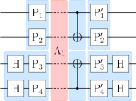
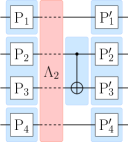
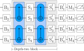
a	b	c	d	e

Fig. S4: Overview of circuit layers and noise-learning circuits. Example four-qubit layers with (a) two cx gates and (b) a single cx gate. These and other gates such as cz and cy are implemented using cx gates in the native direction and flanked with single-qubit gates where needed. The core part of the layer that includes the cx gates is twirled by randomly sampled Paulis $P_{1}P_{2}P_{3}P_{4}$ and their conjugation under the core gates, $P^{\prime}_{1}P^{\prime}_{2}P^{\prime}_{3}P^{\prime}_{4}$. Doing so for the layers in (a) and (b) gives implementations as shown in (c) and (d), respectively, with the noise associated with the core gates illustrated in red. Benchmarking of the layer fidelities is done using circuits (e) where the depth-two block is repeated zero or more times for a given basis $B_{1}B_{2}B_{3}B_{4}$ and with randomly selected readout-mitigation gates $M_{i}$, which are sampled uniformly from identity and $X$ gates. The $S_{i}$ gates are used to control which Paulis are included in the fidelity pairs.

SV.1 Full rankedness of $M$ when dealing with fidelity pairs

Given a layer of non-overlapping two-qubit Clifford gates such that each gate squares to the identity and such that the support of a Pauli and that of the conjugation by the gate overlap (for instance, conjugation of Pauli IX would not result in Pauli XI). This condition is met for commonly used gates such that CX or CZ gates. We would like to construct a Pauli-Lindblad noise model for the qubits that are included in the gates, along with additional qubits for context, if needed. The model terms consist of all unit-weight Paulis supported on the model qubits, as well as all weight-two Paulis supported on pairs of model qubits that are physically connected. We denote the complete list of Pauli terms by $K$. Benchmarking using even number of layer applications allows us to estimate the product of certain fidelity pairs in a SPAM error free manner. Other fidelities can be estimated based on the application of single layers, or based on symmetry assumptions. In order to fit the noise model we assume access to the following fidelity estimates of the Pauli noise channel: (1) for each qubit $i\in[1,n]$ we have access to the fidelities for all unit-weight Paulis $V_{i}=\{X_{i},Y_{i},Z_{i}\}$; and (2) for each connected qubit pair $(i,j)$ we have access to products of fidelities for $P_{1}\in P_{i,j}=\{X_{i}X_{j},X_{i}Y_{j},\ldots,Z_{i}Z_{j}\}$ and corresponding Paulis $P_{2}\in P_{i,j}^{\prime}$ following application of the layer. We assume that the Pauli terms on qubits $i$ and $j$ of $P_{2}$ are either the same as those of $P_{1}$, or change to the identity. This can always be achieved by inserting appropriate single-qubit gates during benchmarking. For qubit pairs $(i,j)$ without a gate but with gates on each of the qubits, $P_{2}$ can have a weight up to four. For pairs with a gate the weight of $P_{2}$ is either one or two. The weight of Paulis $P_{1}$ is always two. Collecting all $V_{i}$ and $P_{1}$ terms in list $B_{1}$ and all $V_{i}$ and $P_{2}$ terms in list $B_{2}$ such that we have the fidelity product for pairs at corresponding locations in the list and setting the list of all model terms as $K=B_{1}$, we have the following result.

Theorem SV.1.

Given $B_{1}$, $B_{2}$ and $K$ as above, then $M=\mathcal{M}(B_{1},K)+\mathcal{M}(B_{2},K)$ is full rank.

Proof.

We consider increasingly large blocks of $M$ and show that each of them is full rank. We start with the subblock corresponding to the unit-weight Paulis. We then add blocks corresponding to qubit pairs that contain a gate, and finally add the qubit pairs that do not contain a gate. Starting with some notation, define by $I_{n}$ the $n\times n$ identity matrix and let

$$Q=\left(\begin{array}[]{ccc}0&1&1\\ 1&0&1\\ 1&1&0\end{array}\right),\quad I=\left(\begin{array}[]{ccc}1&0&0\\ 0&1&0\\ 0&0&1\end{array}\right),\quad e=\left(\begin{array}[]{c}1\\ 1\\ 1\end{array}\right),\quad\mathbb{1}=Q+I=ee^{T}=\left(\begin{array}[]{ccc}1&1&1\\ 1&1&1\\ 1&1&1\end{array}\right).$$

For individual qubits it can be seen that $\mathcal{M}(V_{i},V_{j})$ is $Q$ when $i=j$ and $0$ otherwise. Setting $V=V_{1}\oplus\cdots\oplus V_{n}$, where $\oplus$ denotes list concatenation, it then follows that $\mathcal{M}(V,V)=I_{n}\otimes Q$, which is full rank since both $I_{n}$ and $Q$ are full rank. Next, we show that the matrix remains full rank if we add a single edge with a gate. We illustrate this step on an example with three qubits and add an edge on qubits (1,2). Consider $\mathcal{M}(V\oplus P_{1,2},V\oplus P_{1,2})$, which has the following structure

	$V_{1}$	$V_{2}$	$V_{3}$	$P_{1,2}$
$V_{1}$	$Q$	$0$	$0$	$Q\otimes e^{T}$
$V_{2}$	$0$	$Q$	$0$	$e^{T}\otimes Q$
$V_{3}$	$0$	$0$	$Q$	0
$P_{1,2}$	$Q\otimes e$	$e\otimes Q$	0	$I\otimes Q+Q\otimes I$

We can eliminate the $\mathcal{M}(P_{1,2},V)$ block by subtracting the Kronecker product of row-block for $V_{1}$ by $e$ and the Kronecker product of $e$ with the row-block for $V_{2}$. Doing so changes to lower-right $\mathcal{M}(P_{1,2},P_{1,2})$ block to

$$I\otimes Q+Q\otimes I-Q\otimes\mathbb{1}-\mathbb{1}\otimes Q=I\otimes Q+Q\otimes I-Q\otimes(Q+I)-(Q+I)\otimes Q=-2Q\otimes Q,$$

which is full rank. This means that $M_{1,2}$ is full rank. Now consider $M^{\prime}_{1,2}=\mathcal{M}(V\oplus P_{1,2}^{\prime},V\oplus E_{1,2})$ in which we replaced $P_{1,2}$ by $P^{\prime}_{1,2}$ in the rows. The rows in $M^{\prime}_{1,2}$ corresponding to elements in $E^{\prime}_{1,2}$ that are weight two exactly match those in $M_{1,2}$. The remaining rows correspond to Paulis with weight one and therefore correspond to one of the rows in $V$. Elimination of the lower-left block therefore results in a lower-right block that is $-2Q\otimes Q$, but with some rows zeroed out. The rows we sweep with in $M_{1,2}$ and $M^{\prime}_{1,2}$ are identical, which means we can perform the row sweeps with half the weight in the sum $M_{1,2}+M^{\prime}_{1,2}$. The resulting matrix is $D(Q\otimes Q)$ with diagonal matrix $D$ with terms $-2$ and $-4$. That means that even though $M^{\prime}_{1,2}$ may not be full rank, the sum of the two matrices is. Given that the qubit pairs with gates do not have any overlap we can simply repeat the same procedure for each such pair. Moving on to pairs $(i,j)$ without a gate we note that we can again factor each Pauli term as a product of two Paulis. If there is a gate $(i,i^{\prime})$ then one part of the factorization will be a Pauli supported on either $i$ or $(i,i^{\prime})$. If there is no gate on $i$, then the Pauli is simply supported on $i$. The same applies to qubit $j$ with possible gate $(j,j^{\prime})$. Given that gates do not overlap we never have $i^{\prime}=j^{\prime}$ and the supports of the two factors will therefore always be disjunct. Based on the assumptions we have that corresponding Paulis in $P_{i,j}$ and $P_{i,j}^{\prime}$ have the same term for qubit $i$ and likewise for qubit $j$. That means that $\mathcal{M}(P_{i,j},P_{i,j})=\mathcal{M}(P_{i,j}^{\prime},P_{i,j})=I\otimes Q+Q\otimes I$. If qubit $i$ does not have a gate we sweep the first Pauli factors with a row from $V_{i}$. If qubit $i$ does have an incident gate we can sweep with the appropriate row from the $P_{i,i^{\prime}}$ (or $P_{i^{\prime},i}$) block if the support changes, and otherwise use a row from $V_{i}$. Doing the same for $j$, we see that we can sweep the lower-right block of the new matrix and end up with a combined $-4Q\otimes Q$ lower-right block. As an aside, note that sweeping is done directly on the combined matrix, since all Paulis $P_{i,j}$ on pairs $(i,j)$ with a gate have weight two, whereas we possibly need to sweep with their weight-one counterpart found only in $P_{i,j}^{\prime}$. ∎

SVI Probabilistic error cancellation and error-analysis

The purpose of noise mitigation is to accurately estimate the expectation value of observables. For a circuit consisting of ideal operations $\mathcal{U}_{l}\circ\cdots\circ\mathcal{U}_{1}$, initial state $\rho_{0}$, and observable $A$, which we assume to have an operator norm $\|{A}\|\leq 1$, we would like to estimate

$$\langle A\rangle=\mathrm{Tr}\left[A\,\mathcal{U}_{l}\circ\cdots\circ\mathcal{U}_{1}(\rho_{0})\right].$$

Each of the maps $\mathcal{U}_{i}$ is available only through its noisy version $\tilde{\mathcal{U}}_{i}=\mathcal{U}_{i}\circ\Lambda_{i}$, where $\Lambda_{i}$ is twirled and assumed to be a Pauli-Lindbladian channel. Using the techniques described earlier, we can learn this channel in experiment up to an error as given in Theorem SIV.2 giving rise to the channel estimate $\hat{\Lambda}_{i}$. We can implement the inverse $\hat{\Lambda}_{i}^{-1}$ of this channel estimate in experiment as described in section SVI.1.

SVI.1 Sampling from the inverse

The PEC error mitigation protocol asks that we sample the noise inverse by a quasi-probabilistic technique described in Section SII.2. For the noise process we are working with the Pauli-twirling method as explained in Section SII.1 and learn the resulting sparse noise model following Section SIV. Although our noise model (S9) represents a Pauli channel, it is not in the canonical form shown in (S3). If we denote by $\mathcal{K}$ the set of $k$ values that are included in the noise model, then it is easily seen that there there are $2^{|\mathcal{K}|}$ different products of the identity and $P_{k}$ terms in (S9), each with a possibly different weight. In order to find the coefficient for a certain Pauli $P$ in the canonical representation (S3) we would have to identify and sum up weights of all products that result in this particular Pauli to obtain the right coefficient in the canonical expansion. Moreover, the error-mitigation method asks that we then invert and re-normalized the expansion accordingly. Following these steps as outlined directly is computationally clearly intractable.

Instead, we produce the samples from the inverse by exploiting the product structure of the model (S9). The channel $\Lambda=\mbox{exp}[{\cal L}]$ is given as a product of $|\mathcal{K}|$ individual (commuting), c.f. (S7), Pauli channels $\left(w_{k}\rho+(1-w_{k})P_{k}\rho P_{k}\right)$, with $w_{k}=(1+e^{-2\lambda_{k}})/2$. The inverse of the overall channel then reduces to the product of the individual inverse channels. We can write these inverse channels as $(2w_{k}-1)^{-1}\left(w_{k}\rho-(1-w_{k})P_{k}\rho P_{k}\right)$. The full inverse channel is given then by the product

$$\Lambda^{-1}(\rho)=\gamma\prod_{k\in{\cal K}}\left(w_{k}\cdot-(1-w_{k})P_{k}\cdot P_{k}\right)\rho,$$ (S22)

where the sampling overhead $\gamma$ is given as the product of the individual normalizing factors so that

$$\gamma=\prod_{k\in\mathcal{K}}(2w_{k}-1)^{-1}=\exp\Big{(}\sum_{k\in\mathcal{K}}2\lambda_{k}\Big{)}\;.$$ (S23)

This means the application of the inverse $\Lambda^{-1}(\rho)$ can be sampled according to the following steps. For every $k\in{\cal K}$ we sample the identity matrix with probability $w_{k}$, and $P_{k}$ with probability $1-w_{k}$. Each time we sample a Pauli matrix $P_{k}$, we record the minus sign $(-1)$. To produce a single sample of the full inverse it then suffices to multiply all the (Abelian) Pauli terms we have sampled as well as all observed signs. The final Pauli is then inserted in the random circuit instance and the measurement sample for this instance is then obtained by multiplying the observed outcome with the final sign and the factor $\gamma$. This procedure has to be applied at every layer $i=1,2,\ldots l$ of the circuit, c.f. Fig 1a (main text) so that all these factors compound. This means that the sampling protocol has to be applied to the noise channel $\Lambda_{i}$ for each layer $i=1,2,\ldots,l$. This means that every layer contributes a multiplicative factor of $\gamma_{i}$ to the sampling overhead resulting in the full overhead $\gamma(l)=\prod_{i=1}^{l}\gamma_{i}$. Likewise, we have to record the total number of times $m$ by which we have sampled a Pauli matrix for all the layers, so that we can assign the global sign flip as $(-1)^{m}$. Note, that this sampling procedure does not change the form of the random quantum circuits we need to sample. In fact this error mitigation procedure only uses instances of Pauli-twirled quantum circuits and only modifies the classical distribution from which the circuits are drawn and multiples the output by the factor $(-1)^{m}\gamma(l)$. These additional steps are all taken only in classical pre- and post-processing.

It is also possible to explicitly expand subsets of terms in (S9) and work with Pauli channels that contain more terms. Since combining terms we are able to decrease $\gamma$. This enables us to make a trade-off between the computational complexity of expanding the channels and sample complexity due to scaling parameter $\gamma$.

SVI.2 Error bounds for probabilistic error cancellation

Let us assume for simplicity that observable $A$ can be diagonalized in the computational basis and has eigenvalues $X\in\{-1,+1\}$, as is for example the case for Pauli observables. We absorb the factor $\pm 1$ that originate from the quasi-probability sampling method, c.f. section SVI.1 into the random variable $X$ already. Note, that the general case can be reduced to estimating Pauli-observables or other binary measurements. Furthermore, while considering the error bound for the PEC protocol, we assume that there are no state preparation and readout errors. These can be addressed through other means BER2020MTa-arXiv ; BRA2021SKMa . This means, we can sample $N$ noise-mitigated circuit instances and measure the observable $A$ to obtain $r=1,2\ldots N$ individual samples $X_{r}$. From these, we can estimate the observable expectation value as

$$\langle\hat{A}_{N}\rangle:=\gamma(l)\frac{1}{N}\sum_{r=1}^{N}X_{r}=\gamma(l)\mathbb{E}(X).$$ (S24)

The following Theorem provides a bound on the difference between the actual and estimated expectation value for observable $A$.

Theorem SVI.1.

Assume that all noise channels $\Lambda_{i}$ are learned at each layer $i=1,2,\ldots l$ of the circuit with a multiplicative error as in Theorem SIV.2. Then it holds with probability at least $1-\delta$ for $\delta>0$, that

$$|\langle{A}\rangle-\langle\hat{A}_{N}\rangle|\leq(C_{\epsilon}^{l\tau}-1)+\gamma(l)\sqrt{2\log(2/\delta)/N},$$

where $N$ is the number of error-mitigation circuit instances, $\gamma(l)=\prod_{i=1}^{l}\gamma_{i}$ is the product of the scaling factors $\gamma_{i}$ for the estimated channels $\hat{\Lambda}_{i}$, and $C_{\epsilon}$ and $\tau$ are as in Theorem SIV.2.

To simplify notation throughout the manuscript we have simply referred to the noise channel as $\Lambda$ independently of whether we are dealing with the ideal channel or its estimate $\hat{\Lambda}$ obtained from the noise-learning procedure. To account for a full error analysis we now have to make an explicit distinction. Note however, that crucially both the error-bound in the theorem SVI.1, as well as the quasi-probabilistic noise inversion method in section SVI.1 depend on the estimated value for $\gamma(l)$ obtained from the learning experiments and do not need the knowledge of the ideal values for the exact channel $\Lambda$. Furthermore, we point out that the estimates can naturally be related to the ideal values by Theorem SIV.2.

Proof.

There are two contributions to the error, first the increased sampling error that arises due to the PEC protocol itself and second the error we occur due to errors in the noise-learning procedure that determine the estimate for the $\hat{\Lambda}_{i}$. As discussed in this section, the random variable $X$ in Eq. (S24) satisfies

$$\gamma(l)\mathbb{E}(X)=\mathrm{Tr}\left[A\,\left(\mathcal{U}_{l}\circ\Lambda_{l}\circ\hat{\Lambda}_{l}^{-1}\right)\circ\cdots\circ\left(\mathcal{U}_{1}\circ\Lambda_{1}\circ\hat{\Lambda}_{1}^{-1}\right)(\rho_{0})\right].$$ (S25)

Bounding the right-hand side of Hoeffding’s inequality (S17) by $\delta$ gives an additive error for $\mathbb{E}(X)$ of

$$\epsilon_{s}\leq\sqrt{2\log(2/\delta)/N}$$ (S26)

with probability at least $1-\delta$. This allows us to estimate $\mathbb{E}(X)$ in Eq. (S25) up to an additive sampling error of $\epsilon_{s}$. In order to bound $|\langle A\rangle-\langle\hat{A}\rangle|$, we first define

$$\mathcal{T}_{k}=\mathcal{U}_{k}\circ\cdots\circ\mathcal{U}_{1},\qquad\mbox{and}\qquad\mathcal{S}_{k}=\left(\mathcal{U}_{k}\circ\Lambda_{k}\circ\hat{\Lambda}_{k}^{-1}\right)\circ\cdots\circ\left(\mathcal{U}_{1}\circ\Lambda_{1}\circ\hat{\Lambda}_{1}^{-1}\right).$$

It then follows from the triangle inequality and properties of the trace that

$$|\langle A\rangle-\langle\hat{A}\rangle| \leq\gamma(l)\epsilon_{s}+|\langle A\rangle-\gamma(l)\mathbb{E}(X)|$$

$$=\gamma(l)\epsilon_{s}+|\mathrm{Tr}\left[A\,\mathcal{T}_{l}(\rho_{0})\right]-\mathrm{Tr}\left[A\,\mathcal{S}_{l}(\rho_{0})\right]|$$

$$\leq\gamma(l)\epsilon_{s}+\|A\|\|(\mathcal{T}_{l}-\mathcal{S}_{l})(\rho_{0})\|_{1}$$

$$\leq\gamma(l)\epsilon_{s}+\|{\mathcal{T}_{l}-\mathcal{S}_{l}}\|_{\diamond},$$ (S27)

with $\|{A}\|\leq 1$. The last inequality follows from the definition of the diamond norm $\|{\cdot}\|_{\diamond}$, which has a number of useful, properties.

For TCP-maps $T$ we have $\|{T}\|_{\diamond}\leq 1$, whereas for general linear maps $A$ and $B$ the norm is sub-multiplicative and thus satisfies $\|{A\circ B}\|_{\diamond}\leq\|{A}\|_{\diamond}\|{B}\|_{\diamond}$. For linear maps we therefore have

$$\|{A_{1}\circ A_{2}-B_{1}\circ B_{2}}\|_{\diamond}\leq\|{A_{1}-B_{1}}\|_{\diamond}\|{A_{2}}\|_{\diamond}+\|{B_{1}}\|_{\diamond}\|{A_{2}-B_{2}}\|_{\diamond}.$$ (S28)

Note, that both $\Lambda$ and $\hat{\Lambda}^{-1}$ have diagonal Pauli-transfer matrices. The combined map $\Lambda\circ\hat{\Lambda}^{-1}$ has therefore eigenvalues $f_{j}(\widehat{f_{j}^{-1}})$ that are bounded by $C_{\epsilon}^{-\tau}\leq f_{j}(\widehat{f_{j}^{-1}})\leq C_{\epsilon}^{\tau}$ according to Theorem SIV.2. Hence, we immediately have that $C_{\epsilon}^{-\tau}\leq\|{\Lambda\circ\hat{\Lambda}^{-1}}\|_{\diamond}\leq C_{\epsilon}^{\tau}$. From this it follows that

$$\|{\mathcal{T}_{l}-\mathcal{S}_{l}}\|_{\diamond} =\|{\mathcal{U}_{l}\circ\mathcal{I}d\circ\mathcal{T}_{l-1}-\mathcal{U}_{l}\circ(\Lambda_{l}\circ\hat{\Lambda}_{l}^{-1})\circ\mathcal{S}_{l-1}}\|_{\diamond}$$

$$\leq\|{\mathcal{I}d\circ\mathcal{T}_{l-1}-(\Lambda_{l}\circ\hat{\Lambda}_{l}^{-1})\circ\mathcal{S}_{l-1}}\|_{\diamond}$$

$$\leq\|{\mathcal{I}d-\Lambda_{l}\circ\hat{\Lambda}_{l}^{-1}}\|_{\diamond}\|{\mathcal{T}_{l-1}}\|_{\diamond}+\|{\Lambda_{l}\circ\hat{\Lambda}_{l}^{-1}}\|_{\diamond}\|{\mathcal{T}_{l-1}-\mathcal{S}_{l-1}}\|_{\diamond}$$

$$\leq(C_{\epsilon}^{\tau}-1)+C_{\epsilon}^{\tau}\|{\mathcal{T}_{l-1}-\mathcal{S}_{l-1}}\|_{\diamond}.$$

For the final iteration we can take $\mathcal{T}_{-1}$ and $\mathcal{S}_{-1}$ to be the identity, giving $\|{\mathcal{T}_{1}-\mathcal{S}_{1}}\|_{\diamond}\leq C_{\epsilon}^{\tau}-1$. Solving the resulting recurrence relation gives

$$\|{\mathcal{T}_{l}-\mathcal{S}_{l}}\|_{\diamond}\leq C_{\epsilon}^{l\tau}-1.$$

The result then follows from Eqs. (S26) and (S27). ∎

SVI.3 Weak exponential scaling

Consider a layer consisting of $k$ non-overlapping two-qubit gates such that each gate on qubits $i$, $j$ is affected by a local two-qubit depolarizing channel $\mathcal{D}(\rho)=f\rho+\frac{1-f}{4}\mbox{Tr}_{ij}[\rho]$, such that the fidelity for any Pauli is $f$. For each channel we can form a two-local error model, for which it follows from (S11) that all model coefficient in $\lambda$ are $-\log(f)/16$. Given that the gates do not overlap we can combine the individual noise channel into the layer-level noise channel using the results from Section SIII.1. It is then easy to see that the overall noise model has $15k$ nonzero model coefficients, all equal to $-\log(f)/16$. Using (S23) it then follows that $\gamma=\exp(-(15k/8)\log(f))$. This expression allows us to analyze the growth of $\gamma$ for the Ising model in the main text. For $n$ qubits we have one layer with $\lfloor n/2\rfloor$ gates and one layer with $\lfloor(n-1)/2\rfloor$ gates. In Figure S5a we plot the value of $\gamma$ as a function of $(1-f)$ for different number of qubits $n$. The plot in Figure S5b then shows for $n=50$ the relative number of circuit instances that need to be sampled to attain a similar variance in the estimated observable for different number of Trotter steps. Although the curves rise quickly in the error $(1-f)$, the opposite is also true: minor improvements in gate fidelities lead to a huge decrease in the number of circuit instances that need to be sampled and therefore enable simulation of larger systems.

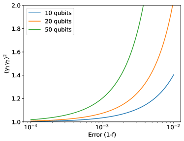
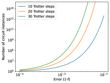
a		b

Fig. S5: Scaling of (a) the sampling overhead factor $\gamma=(\gamma_{1}\gamma_{2})^{2}$ for the Ising simulations discussed in the main text, in case each cx gate is affected by depolarizing noise with fidelity $f$. Plot (b) shows the relative number of circuit instances needed for $n=50$ to achieve a similar variance in estimates. Slight improvements in the gate fidelity lead to significant reductions in the required number of circuit instances.

SVII Setup of the experiment

SVII.1 Devices of the experiment

We performed the experiments on superconducting quantum processors Jurcevic2020 ; Zhang2020-laser-anneal , which utilized fixed-frequency transmon qubits Koch2007 . All devices were patterned to realize heavy-hexagon lattices (see Fig. 1d of the main text). The experiments presented in the main text were all obtained on the same 27-qubit Falcon processor, named ibm_hanoi. Other iterations of the protocol were executed on other Falcon chips (ibm_mumbai, ibm_kolkata, ibm_syndey, and ibm_montreal), with results and conclusions similar to those presented for ibm_hanoi. We view these additional tests as an indicator for the reproducibility and robustness of the protocol.

SVII.2 Specifications of the primary device

Basis gates — All circuits were transpiled to the standard basis gate set $\big{\{}I,\sqrt{X},X,R_{Z},\mathrm{CX}\big{\}}$. The single-qubit gates $\sqrt{X}$ and $X$ were implemented using the standard circuit quantum electrodynamics (cQED) all-microwave-control setup, using Gaussian pulses with calibrated DRAG decoupling Motzoi2009 ; JChow2010-DRAG , each with a total gate time of 35.5 ns (4$\sigma$ Gaussian pulses). The $I$ and $R_{Z}$ pulses were virtualized PhysRevA.96.022330 , and hence took no time. The two-qubit CX gates were implemented using cross-resonance pulses Paraoanu2006 ; Chow2011 with gate times optimized to maximize fidelity. Figure S6 shows the chip topology of ibm_hanoi along with the duration of its CX gates in their native direction. The CX gate duration ranges from 181 to 519 ns, and their average error, as estimated by randomized benchmarking, was 0.98%. In all experiments, the qubits were cooled to the ground state prior to the start of the protocol.

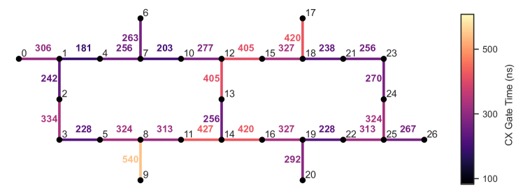
Fig. S6: Quantum processor topology and native CX gate duration for ibm_hanoi. Each node represents a qubit and is labeled by the physical qubit number (black text). CX Gates are represented by edges, along with their gate time in nanoseconds (colored text).

Coherence — Processor ibm_hanoi had a quantum volume of 64 Jurcevic2020 and average energy-relaxation $T_{1}$ and Hanh echo $T_{2}^{E}$ times of $151\,\mathrm{\mu s}$ and $107\,\mathrm{\mu s}$, respectively. As typical for supercomputing qubits Klimov2018 ; Carroll2021 , these times fluctuated over the duration of the experiments. In Fig. S7, we summarize the distribution of the variations in $T_{2}^{E}$ over a two-month long period for each of the 27 qubits. We limited the effects of temporal fluctuations by interleaving our mitigation experiments with noise-learning runs every few hours.

Readout — We define the readout assignment fidelity per qubit as $\mathcal{F}_{a}=1-{\textstyle\frac{1}{2}}\left(P(1\,|\,0)+P(0\,|\,1)\right),$ where $P(A\,|\,B)$ is the empirical probability to measure the qubit in state $A\in\{0,1\}$ given that the qubit was nominally prepared in state $B\in\left\{0,1\right\}$. The average assignment readout error $1-\mathcal{F}_{a}$ across all qubits in our device was $2.5\%$. We note that the probability distribution is biased due to energy relaxation such that $P(1\,|\,0)<P(0\,|\,1)$.

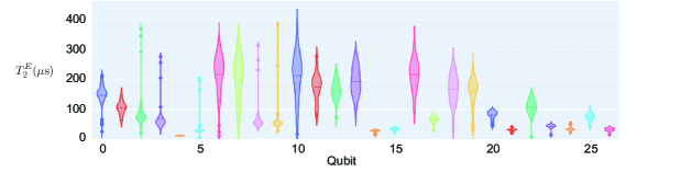
Fig. S7: Device coherences and time variability. Distribution of the $T_{2}$-echo relaxation times for each of the qubits of device ibm_hanoi over a two-month period, depicted as a violin plot. A larger horizontal width of the violin plot indicates a larger probability of sampling this $T_{2}^{E}$ time. The horizontal dashed lines indicate the mean of the distribution.

	Symbol	Value
Quantum volume	$\mathrm{QV}$	$64$
Energy relaxation lifetime	$T_{1}$	$151\,\mathrm{\mu s}$
Hanh echo time	$T_{2}^{E}$	$107\,\mathrm{\mu s}$
Readout assignment error	$1-\mathcal{F}_{a}$	$2.5\%$
CX error		0.98%

Table 1: Summary table of average device metrics for ibm_hanoi. Symbols explained in Sec. SVII.2.

SVII.3 Dynamical decoupling

As a result of the different gate times, qubits in our layer of CX gates can experience idle periods. This holds especially true for context qubits, which are idle for the full duration of the layer. To lessen the effects of decoherence and low-frequency noise during these idle periods, we apply dynamical decoupling (DD) Viola1999 ; Zanardi1999 , which was recently demonstrated to improve circuit fidelity Jurcevic2020 . For dynamical decoupling we use a standard $X_{p}-X_{m}$ sequence, which is the simplest version of a Car-Purcell-Meiboom-Gill (CPMG) echo train Carr1954 ; Meiboom1958 . This is illustrated in Fig. S8.

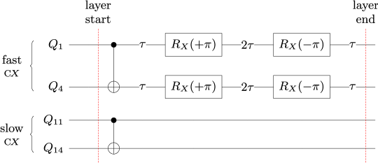
Fig. S8: Dynamical decoupling inside a layer. Structure of a simple dynamical decoupling sequence used during idle qubit times, illustrated on a four-qubit layer with concurrent cx gates on qubits $1-4$ and $11-14$. The delay duration $\tau$ is calculated as the idle time minus the duration of the two $R_{X}$ gates, divided by four.

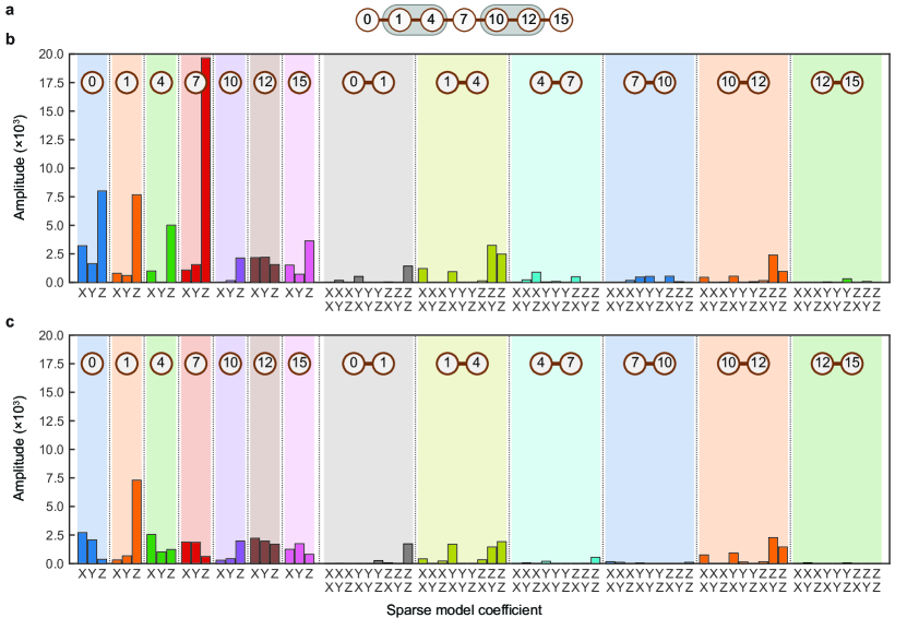
Fig. S9: Noise model coefficients in the presence and absence of dynamical decoupling. (a) Schematic depiction of a 7-qubit layer on ibm_kolkata with cx gates on qubits $1-4$ and $10-12$, and (idle) context qubits 0, 7, and 15. (b,c) Plots of the learned noise-model coefficients in the absence (b) and presence (c) of dynamical decoupling within the layer using an $X_{p}-X_{m}$ sequence on the context qubits. The numbered circles overlaid over each section of the bar plots indicate the support of the model Pauli terms.

To study the effect of dynamical decoupling on the structure of noise in our system, we considered a 7-qubit layer with two CX gates and three (idle) context qubits, as illustrated in Fig. S9a. We then learned the layer with and without dynamical decoupling applied to the context qubits. The noise model coefficients obtained without dynamic decoupling are shown in Fig. S9b. The dominant noise in the system corresponds to unit-weight Pauli-Z terms. The origin of these dominant noise terms may be attributed to $T_{2}$ qubit dephasing and other coherent $Z$-noise arising from crosstalk. Repeating the experiment with dynamical decoupling enabled resulted in the model coefficients shown in Fig. S9c. It is seen that the large Pauli-Z noise terms on the idle qubits are significantly reduced.

SVII.4 Additional learning and control experiments

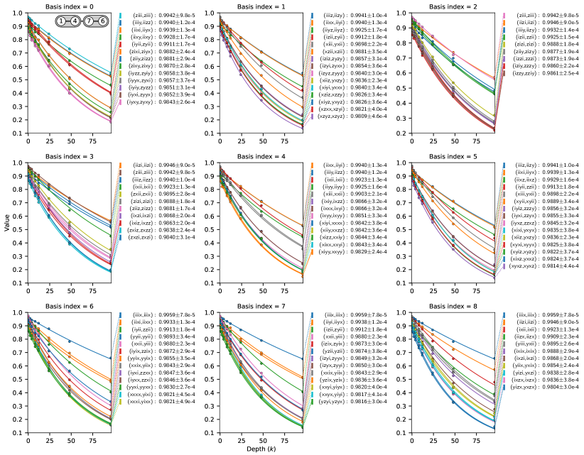
Fig. S10: Raw data of noise-learning experiments. Plots of the learning data in all nine different bases for the four-qubit layer of Fig. 2a of the main text. The layer consists of two concurrent cx gates applied to qubits 1–4 and 7–6 on ibm_hanoi (see top-left inset). Each plot gives the observable expectation values for different circuit depths along with the exponentially decaying function fitted through the data points, with decay rate corresponding to the square root of the product of two fidelities. Fitting for a given fidelity pair is done for all occurrences within and across the different bases. For instance the fidelity for ziii is determined based on the data obtained for basis indices 0 and 2, whereas the fidelity pair iyii–zyii occurs twice for basis index 0.

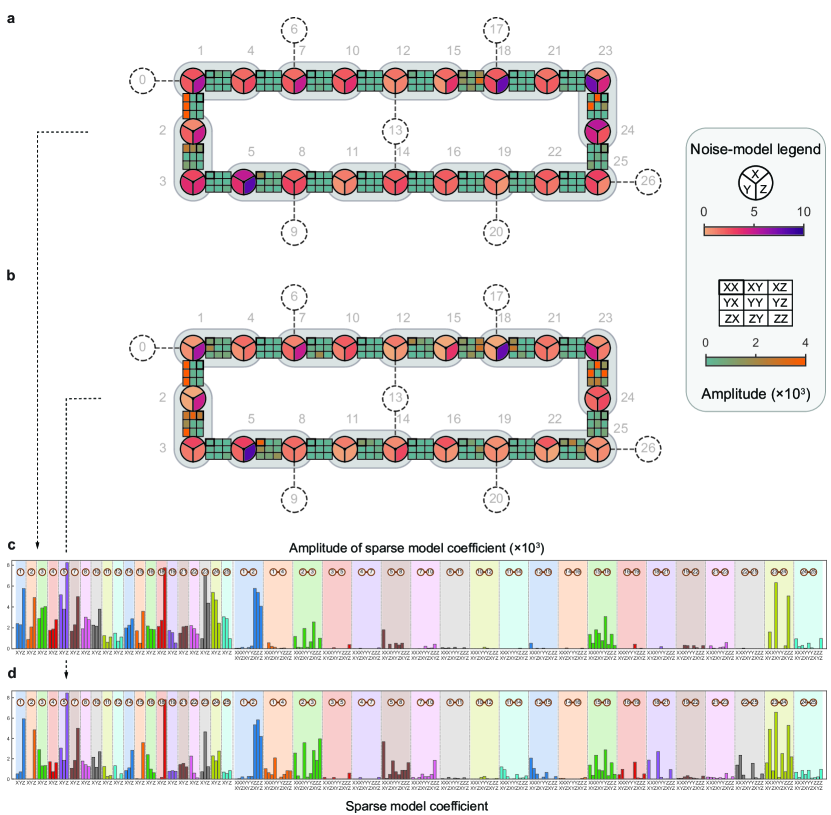
Fig. S11: Comparison between unit-depth and symmetry noise model fitting. Panels (a) and (b) depict the ibm_hanoi processor topology along with a 20-qubit layer consisting of 10 cx gates. We learn the noise model using (a) unit-depth circuits and (b) using a symmetry assumption on the noise channel. The resulting weight-one Pauli generators (X, Y, Z terms) in the Lindblad model are given as wedges inside the circular qubit nodes. Similarly, the weight-two Pauli generators (XX, XY, and so on) in the Lindblad model are visualized by the $3\times 3$ grids connecting pairs of qubits. The legend on the right shows the corresponding color bar detailing the noise amplitude. Panels (c) and (d) present the same data (see down-pointing arrows) as bar plot of the noise-model coefficients.

In Fig. S10 we provide the full data for the noise-model learning setup of Fig. 2a in the main text, as measured in all nine bases determined by the learning protocol.

Finally, in Fig. S11, we compare the noise model extracted using the unit-depth and symmetric learning post-processing methods for a 20 qubit layer with 10 cx gates. The bottom panels of the figure show the noise-model coefficients obtained using the unit-depth and symmetric methods, respectively. Aside from some localized differences, the profiles of the two noise models were found to match well overall. For all experiments in this work, aside from the present one, we used symmetry-based model fitting.

References

- (1) Zhang, E. J. et al. High-fidelity superconducting quantum processors via laser-annealing of transmon qubits. arXiv:2012.08475 (2020).
- (2) Arute, F. et al. Quantum supremacy using a programmable superconducting processor. Nature 574, 505–510 (2019).
- (3) Wu, Y. et al. Strong quantum computational advantage using a superconducting quantum processor. Phys. Rev. Lett. 127, 180501 (2021).
- (4) Peruzzo, A. et al. A variational eigenvalue solver on a photonic quantum processor. Nature communications 5, 1–7 (2014).
- (5) Kandala, A. et al. Hardware-efficient variational quantum eigensolver for small molecules and quantum magnets. Nature 549, 242–246 (2017).
- (6) Kim, Y. et al. Scalable error mitigation for noisy quantum circuits produces competitive expectation values. arXiv:2108.09197 (2021).
- (7) Havlíček, V. et al. Supervised learning with quantum-enhanced feature spaces. Nature 567, 209–212 (2019).
- (8) Schuld, M. & Killoran, N. Quantum machine learning in feature Hilbert spaces. Physical review letters 122, 040504 (2019).
- (9) Temme, K., Bravyi, S. & Gambetta, J. M. Error mitigation for short-depth quantum circuits. Physical Review Letters 119, 180509 (2017).
- (10) Li, Y. & Benjamin, S. C. Efficient variational quantum simulator incorporating active error minimization. Phys. Rev. X 7, 021050 (2017).
- (11) Kandala, A. et al. Error mitigation extends the computational reach of a noisy quantum processor. Nature 567, 491–495 (2019).
- (12) Endo, S., Benjamin, S. C. & Li, Y. Practical quantum error mitigation for near-future applications. Physical Review X 8, 031027 (2018).
- (13) Guo, Y. & Yang, S. Quantum error mitigation via matrix product operators. arXiv preprint arXiv:2201.00752 (2022).
- (14) Piveteau, C., Sutter, D. & Woerner, S. Quasiprobability decompositions with reduced sampling overhead. arXiv:2101.09290 (2021).
- (15) Endo, S., Cai, Z., Benjamin, S. C. & Yuan, X. Hybrid quantum-classical algorithms and quantum error mitigation. Journal of the Physical Society of Japan 90, 032001 (2021).
- (16) Piveteau, C., Sutter, D., Bravyi, S., Gambetta, J. M. & Temme, K. Error mitigation for universal gates on encoded qubits. arXiv:2103.04915 (2021).
- (17) Takagi, R. Optimal resource cost for error mitigation. Phys. Rev. Research 3, 033178 (2021).
- (18) Takagi, R., Endo, S., Minagawa, S. & Gu, M. Fundamental limits of quantum error mitigation. arXiv:2109.04457 (2021).
- (19) Song, C. et al. Quantum computation with universal error mitigation on a superconducting quantum processor. Science Advances 5, eaaw5686 (2019).
- (20) Zhang, S. et al. Error-mitigated quantum gates exceeding physical fidelities in a trapped-ion system. Nature Communications 11, 587 (2020).
- (21) Strikis, A., Qin, D., Chen, Y., Benjamin, S. C. & Li, Y. Learning-based quantum error mitigation. PRX Quantum 2, 040330 (2021).
- (22) Bennett, C. H. et al. Purification of noisy entanglement and faithful teleportation via noisy channels. Phys. Rev. Lett. 76, 722–725 (1996). URL https://link.aps.org/doi/10.1103/PhysRevLett.76.722.
- (23) Knill, E. Fault-tolerant postselected quantum computation: Threshold analysis. arXiv:quant-ph/0404104 (2004).
- (24) Kern, O., Alber, G. & Shepelyansky, D. L. Quantum error correction of coherent errors by randomization. The European Physical Journal D-Atomic, Molecular, Optical and Plasma Physics 32, 153–156 (2005).
- (25) Geller, M. R. & Zhou, Z. Efficient error models for fault-tolerant architectures and the Pauli twirling approximation. Physical Review A 88, 012314 (2013).
- (26) Wallman, J. J. & Emerson, J. Noise tailoring for scalable quantum computation via randomized compiling. Physical Review A 94, 052325 (2016).
- (27) Breuer, H.-P. & Petruccione, F. The theory of open quantum systems (Oxford University Press, 2002).
- (28) Flammia, S. T. & Wallman, J. J. Efficient estimation of Pauli channels. ACM Transactions on Quantum Computing 1 (2020).
- (29) Erhard, A. et al. Characterizing large-scale quantum computers via cycle benchmarking. Nature Communications 10, 1–7 (2019).
- (30) Kimmel, S., da Silva, M. P., Ryan, C. A., Johnson, B. R. & Ohki, T. Robust extraction of tomographic information via randomized benchmarking. Phys. Rev. X 4, 011050 (2014).
- (31) Helsen, J., Xue, X., Vandersypen, L. M. K. & Wehner, S. A new class of efficient randomized benchmarking protocols. npj Quantum Information 5, 1–9 (2019).
- (32) Harper, R., Flammia, S. T. & Wallman, J. J. Efficient learning of quantum noise. Nature Physics 16, 1184–1188 (2020).
- (33) van den Berg, E., Minev, Z. & Temme, K. Model-free readout-error mitigation for quantum expectation values. arXiv:2012.09738 (2020).
- (34) Wack, A. et al. Quality, speed, and scale: three key attributes to measure the performance of near-term quantum computers (2021). eprint 2110.14108.
- (35) Bravyi, S., Sheldon, S., Kandala, A., McKay, D. & Gambetta, J. M. Mitigating measurement errors in multiqubit experiments. Physical Review A 103, 042605 (2021).
- (36) Chen, S., Yu, W., Zeng, P. & Flammia, S. T. Robust shadow estimation. arXiv:2011.09636 (2020).
- (37) Aaronson, S. & Gottesman, D. Improved simulation of stabilizer circuits. Physical Review A 70, 052328 (2004).
- (38) Cai, Z. & Benjamin, S. C. Constructing smaller Pauli twirling sets for arbitrary error channels. Scientific reports 9, 1–11 (2019).
- (39) Bravyi, S. & Maslov, D. Hadamard-free circuits expose the structure of the Clifford group. arXiv:2003.09412 (2020).
- (40) Jurcevic, P. et al. Demonstration of quantum volume 64 on a superconducting quantum computing system. Quantum Science and Technology 6 (2020).
- (41) Zhang, E. J. et al. High-fidelity superconducting quantum processors via laser-annealing of transmon qubits. arXiv:2012.08475 (2020).
- (42) Koch, J. et al. Charge-insensitive qubit design derived from the Cooper pair box. Physical Review A 76, 42319 (2007).
- (43) Motzoi, F., Gambetta, J. M., Rebentrost, P. & Wilhelm, F. K. Simple pulses for elimination of leakage in weakly nonlinear qubits. Physical Review Letters 103, 110501 (2009).
- (44) Chow, J. M. et al. Optimized driving of superconducting artificial atoms for improved single-qubit gates. Physical Review A 82, 040305 (2010).
- (45) McKay, D. C., Wood, C. J., Sheldon, S., Chow, J. M. & Gambetta, J. M. Efficient gates for quantum computing. Phys. Rev. A 96, 022330 (2017). URL https://link.aps.org/doi/10.1103/PhysRevA.96.022330.
- (46) Paraoanu, G. S. Microwave-induced coupling of superconducting qubits. Physical Review B 74, 140504 (2006).
- (47) Chow, J. M. et al. Simple all-microwave entangling gate for fixed-frequency superconducting qubits. Physical Review Letters 107, 080502 (2011).
- (48) Klimov, P. V. et al. Fluctuations of energy-relaxation times in superconducting qubits. Physical Review Letters 121 (2018).
- (49) Carroll, M., Rosenblatt, S., Jurcevic, P., Lauer, I. & Kandala, A. Dynamics of superconducting qubit relaxation times. arXiv:2105.15201 (2021).
- (50) Viola, L., Knill, E. & Lloyd, S. Dynamical decoupling of open quantum systems. Physical Review Letters 82, 2417 (1999).
- (51) Zanardi, P. Symmetrizing evolutions. Physics Letters A 258, 77–82 (1999).
- (52) Carr, H. Y. & Purcell, E. M. Effects of diffusion on free precession in nuclear magnetic resonance experiments. Physical Review 94, 630 (1954).
- (53) Meiboom, S. & Gill, D. Modified spin-echo method for measuring nuclear relaxation times. RScI 29, 688–691 (1958).