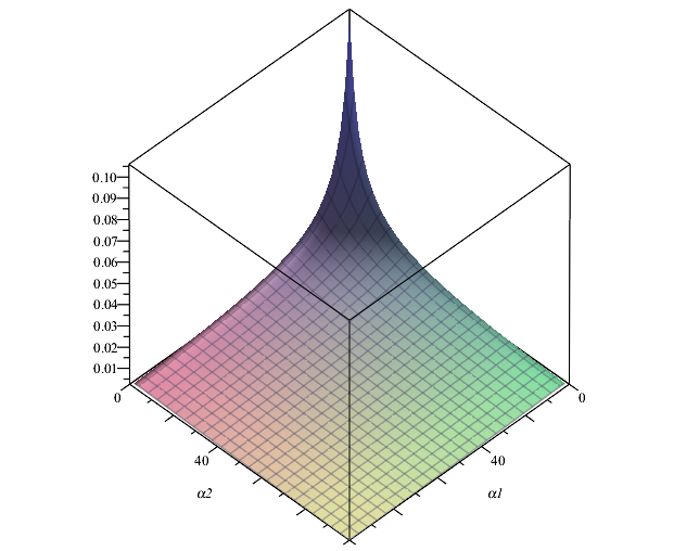
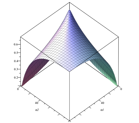
Analytic Mutual Information in Bayesian Neural Networks

Abstract

Bayesian neural networks have successfully designed and optimized a robust neural network model in many application problems, including uncertainty quantification. However, with its recent success, information-theoretic understanding about the Bayesian neural network is still at an early stage. Mutual information is an example of an uncertainty measure in a Bayesian neural network to quantify epistemic uncertainty. Still, no analytic formula is known to describe it, one of the fundamental information measures to understand the Bayesian deep learning framework. In this paper, we derive the analytical formula of the mutual information between model parameters and the predictive output by leveraging the notion of the point process entropy. Then, as an application, we discuss the parameter estimation of the Dirichlet distribution and show its practical application in the active learning uncertainty measures by demonstrating that our analytical formula can improve the performance of active learning further in practice.

I Introduction

Uncertainty quantification plays a crucial role in managing and controlling exposed risks during optimization and decision-making in modern machine learning problems as the trained system is getting more complicated [1, 2, 3, 4]. Bayesian approximation [5, 6] and ensemble learning methods [7, 8, 9] are two of the most widespread techniques to quantify uncertainties in the deep learning literature. The Bayesian neural network typically assumes a stochastic design to produce a posterior probability given prior knowledge. For example, the variational encoding approach is widely adopted [10]. The most straightforward Bayesian approximation is leveraging dropout layers [11]. Another way is applying Laplace approximation [12, 13].

However, with its recent success, information-theoretic understanding about the Bayesian neural network is still at an early stage. Mutual information is an example of an uncertainty measure to quantify epistemic uncertainty [14]. Another conditional entropy term is an example of an aleatoric uncertainty. Both uncertainty measures are practically crucial to evaluate the confidence or fairness of the model. For example, epistemic uncertainty captures the model uncertainty (lack of knowledge), and aleatoric uncertainty captures the inherent data uncertainty. Still, no analytic formulas are known to describe them [15, 11], which are fundamental information measures to understand the Bayesian deep learning framework.

In this paper, we derive the analytical formula of the mutual information between model parameters and the predictive output by leveraging the notion of the point process entropy [16] and assuming that the intermediate encoded message in the Bayesian neural network follows a Dirichlet distribution since Dirichlet distribution family is the most natural and flexible family of probability distributions over a simplex in classification problem. Then, as a direct application, we discuss the parameter estimation of Dirichlet distribution and show its practical application in the active learning uncertainty measures by demonstrating that our analytical formula can improve the performance of active learning further in practice.

II Information-Theoretic Formulation of Bayesian Neural Networks

For simplicity, throughout this paper, we consider a classification problem with a Bayesian neural network approximated by Monte-Carlo (MC) dropouts [6, 11]. However, we note that our analytic framework does not have to be confined to the dropout regime. For example, our proposed framework can also be generalized to Gaussian process [17, 18, 19] or to leverage Laplace approximation in neural network [20, 21].

In an information-theoretic point of view, we can simplify the Bayesian neural network $\Phi\left(\cdot,\omega\right)$ with stochastic model parameters $\omega$ as an encoder-decoder communication channel. Given the data $\mathbf{x}$, the sender sends a message $\left(\mathbf{x},\omega\right)$ equipped with model parameters $\omega$ through the Bayesian channel, then the receiver receives a message $Y\left(\mathbf{x},\omega\right)$ through the decoder. Figure 1 illustrates a diagram in this communication process.

Figure 1: Bayesian neural network channel framework

Under this framework, the Bayesian deep neural network $\Phi$ produces the intermediate prediction probability for a data point $\mathbf{x}$:

$${\Phi}\left(\mathbf{x},\omega\right):=\left(P_{1}(\mathbf{x},\omega),\cdots,P_{C}(\mathbf{x},\omega)\right)\in\Delta^{C},$$

where $\Delta^{C}=\{(p_{1},\cdots,p_{C}):p_{1}+\cdots+p_{C}=1,p_{i}\geq 0\text{ for each }i\}$ and $C$ is the number of classes. For the final class output $Y$, it is assumed to be a multinoulli distribution (or categorical distribution):

$$Y(\mathbf{x},\omega):=\begin{cases}1&\text{with probability $P_{1}(\mathbf{x},\omega)$}\\ \vdots&\vdots\\ C&\text{with probability $P_{C}(\mathbf{x},\omega)$}.\end{cases}$$

Similar to find the channel capacity of the AWGN communication channel under power constraints [22], one may ask a similar question about the capacity of this Bayesian channel which is the mutual information between the model parameters $\omega$ and the output $Y$ denoting by $\mathfrak{I}\left(\omega,Y\left(\mathbf{x},\omega\right)\right)$ given $\mathbf{x}$, a.k.a. $\text{BALD}[\mathbf{x}]$ [23, 15, 24]. In practice, controlling $\omega$ is not straightforward, but we can control the family of the encoded messages $\Phi\left(\mathbf{x},\omega\right)$ in a tractable manner [24, 10, 25]. Since $Y(\mathbf{x},\omega)$ only depends on $\Phi(\mathbf{x},\omega)$, by focusing on $\Phi\left(\mathbf{x},\omega\right)$, we may estimate the mutual information between the model parameters and the channel output [24]:

$$\text{BALD}[\mathbf{x}]:=\mathfrak{I}\left(\omega,Y\left(\mathbf{x},\omega\right)\right)$$ (1)

$$= H(Y\left(\mathbf{x},\omega\right))-\mathbb{E}_{\omega}\left[H\left(Y\left(\mathbf{x},\omega\right)|\omega\right)\right]$$ (2)

$$= H(Y\left(\mathbf{x},\omega\right))-\mathbb{E}_{\Phi}\left[H\left(Y\left(\mathbf{x},\omega\right)|\Phi\left(\mathbf{x},\omega\right)\right)\right]$$ (3)

$$= \mathfrak{I}\left(\Phi\left(\mathbf{x},\omega\right),Y(\mathbf{x},\omega)\right),$$ (4)

where $H(Y\left(\mathbf{x},\omega\right))$ represents the Shannon entropy by marginalizing out the randomness of $\omega$ in $Y\left(\mathbf{x},\omega\right)$ and $\mathfrak{I}(\cdot,\cdot)$ represents a mutual information between two quantities. We remark that the equation (3) is used to numerically estimate $\text{BALD}[\mathbf{x}]$ [24, 26].

The formulations of the mutual information (1) - (4) look natural, but we note that $\omega$ or $\Phi\left(\mathbf{x},\omega\right)$ is on a continuous domain, and $Y(\mathbf{x},\omega)$ is on a discrete domain. This combined domain implies that we cannot directly apply Shannon entropy and differential entropy notions. One immediate question is what the joint entropy between $\Phi\left(\mathbf{x},\omega\right)$ and $Y(\mathbf{x},\omega)$ is. Therefore, we first need to have a generalized notion of the entropy measures fitting into this Bayesian neural network framework.

By leveraging the point process entropy [27, 28, 29, 30, 16], we can generalize the notion of the entropy in this combined domain. We note that a notion of the entropy for a discrete-continuous mixture can be applied in this Bayesian neural network [31]. But the discrete-continuous mixture is a limited case of a point process, i.e., the point process entropy is a generalized definition of the discrete-continuous mixture entropy. Therefore, we keep the notion of the point process entropy in this paper. So equipping with the point process entropy, we need to consider a generalized notion of probability distribution on the combined domain, a.k.a. Jannosy density function [30]. Following the usual point process entropy calculation, we may write a Janossy density function of $\left(\Phi\left(\mathbf{x},\omega\right),Y\left(\mathbf{x},\omega\right)\right)$ on $\Delta^{C}\times[C]$ as follows:

$$j\left(\mathbf{p},y=i\right)=p_{i}f\left(\mathbf{p}\right),$$ (5)

where $\mathbf{p}:=\left(p_{1},\cdots,p_{C}\right)$ and $f(\cdot)$ is a density function of $\Phi\left(\mathbf{x},\omega\right)$. Then the joint entropy of $\Phi\left(\mathbf{x},\omega\right)$ and $Y(\mathbf{x},\omega)$ can be defined as

$$\mathfrak{H}\left(\Phi\left(\mathbf{x},\omega\right),Y\left(\mathbf{x},\omega\right)\right)$$

$$= -\sum_{i=1}^{C}\int_{\Delta^{c}}j\left(\mathbf{p},y=i\right)\log j\left(\mathbf{p},y=i\right)\text{d}\mathbf{p}.$$ (6)

By plugging (5) into (II), we can further drive the following identities:

$$\mathfrak{H}\left(\Phi\left(\mathbf{x},\omega\right),Y\left(\mathbf{x},\omega\right)\right)$$

$$= H\left(Y\left(\mathbf{x},\omega\right)\right)+\mathbb{E}_{Y}\left[h\left(\Phi\left(\mathbf{x},\omega\right)|Y\left(\mathbf{x},\omega\right)\right)\right]$$

$$= h\left(\Phi\left(\mathbf{x},\omega\right)\right)+\mathbb{E}_{\Phi}\left[H\left(Y\left(\mathbf{x},\omega\right)|\Phi\left(\mathbf{x},\omega\right)\right)\right],$$

where $h(\cdot)$ represents the usual differential entropy. Therefore we may further write equivalent forms of the mutual information as follows:

$$(4) =h\left(\Phi\left(\mathbf{x},\omega\right)\right)+H\left(Y\left(\mathbf{x},\omega)\right)\right)-\mathfrak{H}\left(\Phi\left(\mathbf{x},\omega\right),Y(\mathbf{x},\omega)\right),$$ (7)

$$=h\left(\Phi\left(\mathbf{x},\omega\right)\right)-\mathbb{E}_{Y}\left[h\left(\Phi\left(\mathbf{x},\omega\right)|Y\left(\mathbf{x},\omega\right)\right)\right]$$

Then, to establish the analytical formula, we assume that the distribution of $\Phi\left(\mathbf{x},\omega\right)$ follows Dirichlet distribution. In Bayesian model, the Gaussian-softmax-Dirichlet regime is a natural sequential application to generate a classification probability, by applying multivariate Gaussian to soft-max operation, then approximating it to Dirichlet distribution. Therefore, our choice of Dirichlet distribution is widely adopted in the literature of Monte-Carlo dropouts, Laplace approximation-based neural networks, and any Gaussian processes [32, 20, 17, 19, 33].

III Main Results

(a) Analytic epistemic uncertainty (mutual information)

(b) Analytic aleatoric uncertainty (conditional entropy)

Figure 2: Analytic uncertainties when $C=2$, i.e., $\Phi\left(\mathbf{x},\omega\right)\sim\text{Beta}\left(\alpha_{1},\alpha_{2}\right)$ (=Beta distribution). Epistemic uncertainty tends to increase as $\alpha_{1},\alpha_{2}\to 0$, and aleatoric uncertainty tends to increase as $\alpha_{1},\alpha_{2}\to+\infty$.

In this section, we state our main results regarding the analytical form of the mutual information and its variant between model parameters $\omega$ and the predictive output $Y$ of Bayesian neural networks. The key assumption in our result is that the encoded message $\Phi\left(\mathbf{x},\omega\right)$ follows Dirichlet distribution with positive parameters $\left(\alpha_{1},\cdots,\alpha_{C}\right)$. For the sake of brevity, let $\boldsymbol{\alpha}=\left(\alpha_{1},\cdots,\alpha_{C}\right)$ and $\boldsymbol{\alpha}(i,++)=\left(\alpha_{1},\cdots,\alpha_{i-1},\alpha_{i}+1,\alpha_{i+1},\cdots,\alpha_{C}\right)$.

First we note that the entropy term can be decomposed into two uncertainty as below. The mutual information captures the epistemic uncertainty, and the conditional entropy captures the aleatoric uncertainty.

$$H(Y\left(\mathbf{x},\omega\right))=\underbrace{\mathfrak{I}\left(\omega,Y\left(\mathbf{x},\omega\right)\right)}_{\text{epistemic uncertainty}}+\underbrace{\mathbb{E}_{\omega}\left[H\left(Y\left(\mathbf{x},\omega\right)|\omega\right)\right]}_{\text{aleatoric uncertainty}}.$$ (8)

The epistemic uncertainty captures the model uncertainty (lack of knowledge), and the aleatoric uncertainty captures the data uncertainty [14]. The decomposition (8) implies the analytic formula of the aleatoric uncertainty as well. Our main results are Theorem III.1 and Corollary III.2 for both uncertainties.

Theorem III.1.

Assume that $\Phi\left(\mathbf{x},\omega\right):=\left(P_{1},\cdots,P_{C}\right)\sim\text{Dirichlet}(\alpha_{1},\cdots,\alpha_{C})$. Then the mutual information $\mathfrak{I}_{\text{Dirichlet}}\left(\omega,Y(\mathbf{x},\omega)\right)$ can be analytically calculated as follows.

$$\mathfrak{I}_{\text{Dirichlet}}\left(\omega,Y(\mathbf{x},\omega)\right)=\mathfrak{I}_{\text{Dirichlet}}\left(\Phi\left(\mathbf{x},\omega\right),Y(\mathbf{x},\omega)\right)$$

$$= \left(\sum_{k=1}^{C}\alpha_{k}-C\right)\Psi\left(\sum_{k=1}^{C}\alpha_{k}\right)-\sum_{i=1}^{C}\left(\alpha_{i}-1\right)\Psi\left(\alpha_{i}\right)$$

$$- \sum_{i=1}^{C}\left(\frac{\alpha_{i}}{\sum_{k=1}^{C}\alpha_{k}}\right)\log\left(\frac{\alpha_{i}}{\sum_{k=1}^{C}\alpha_{k}}\right)$$

$$+ \sum_{i=1}^{C}\sum_{j\neq i}\frac{\left(\alpha_{j}-1\right)B\left(\boldsymbol{\alpha}(i,++)\right)}{B\left(\boldsymbol{\alpha}\right)}\left[\Psi\left(\alpha_{j}\right)-\Psi\left(\left(\sum_{k=1}^{C}\alpha_{k}\right)+1\right)\right]$$

$$+ \sum_{i=1}^{C}\frac{\alpha_{i}B\left(\boldsymbol{\alpha}(i,++)\right)}{B\left(\boldsymbol{\alpha}\right)}\left[\Psi\left(\alpha_{i}+1\right)-\Psi\left(\left(\sum_{k=1}^{C}\alpha_{k}\right)+1\right)\right],$$

where $B\left(\boldsymbol{\alpha}\right)=\frac{\Gamma(\alpha_{1})\cdots\Gamma(\alpha_{C})}{\Gamma\left(\sum_{k=1}^{C}\alpha_{k}\right)}$, $\Gamma(\cdot)$ is a Gamma function, and $\Psi(\cdot)$ is a Digamma function.

Corollary III.2.

Given the Bayesian neural network with $\Phi\left(\cdot,\omega\right)$, the aleatoric uncertainty can be analytically calculated as follows.

$$\text{Aleatoric uncertainty}\left[\mathbf{x}\right]:=\mathbb{E}_{\omega}\left[H\left(Y\left(\mathbf{x},\omega\right)|\omega\right)\right]$$

$$= -\left(\sum_{k=1}^{C}\alpha_{k}-C\right)\Psi\left(\sum_{k=1}^{C}\alpha_{k}\right)+\sum_{i=1}^{C}\left(\alpha_{i}-1\right)\Psi\left(\alpha_{i}\right)$$

$$- \sum_{i=1}^{C}\sum_{j\neq i}\frac{\left(\alpha_{j}-1\right)B\left(\boldsymbol{\alpha}(i,++)\right)}{B\left(\boldsymbol{\alpha}\right)}\left[\Psi\left(\alpha_{j}\right)-\Psi\left(\left(\sum_{k=1}^{C}\alpha_{k}\right)+1\right)\right]$$

$$- \sum_{i=1}^{C}\frac{\alpha_{i}B\left(\boldsymbol{\alpha}(i,++)\right)}{B\left(\boldsymbol{\alpha}\right)}\left[\Psi\left(\alpha_{i}+1\right)-\Psi\left(\left(\sum_{k=1}^{C}\alpha_{k}\right)+1\right)\right].$$

Figures 2(a) and 2(b) illustrate the behavior of two uncertainties along parameters of Dirichlet distribution when $C=2$.

IV Proof of Theorem III.1

First, we note that the density function $f(\cdot)$ of $\text{Dirichlet}(\alpha_{1},\cdots,\alpha_{C})$ is given by

$$f\left(p_{1},\cdots,p_{C}\right)=\frac{1}{B\left(\boldsymbol{\alpha}\right)}\prod_{i=1}^{C}p_{i}^{\alpha_{i}-1}.$$ (9)

Then to derive the analytical form, we shall calculate each term in the equation (7).

$$\mathfrak{I}_{\text{Dirichlet}}\left(\Phi\left(\mathbf{x},\omega\right),Y(\mathbf{x},\omega)\right)$$

$$= h\left(\Phi\left(\mathbf{x},\omega\right)\right)+H(Y\left(\mathbf{x},\omega\right))-\mathfrak{H}_{\text{Dirichlet}}\left(\Phi\left(\mathbf{x},\omega\right),Y(\mathbf{x},\omega)\right).$$

Given $\Phi\left(\mathbf{x},\omega\right):=\left(P_{1},\cdots,P_{C}\right)\sim\text{Dirichlet}(\alpha_{1},\cdots,\alpha_{C})$, the first differential entropy of Dirichlet distribution is well-known [34, 35].

$$h\left(\Phi\left(\mathbf{x},\omega\right)\right)= -\int_{\Delta^{C}}f\left(\mathbf{p}\right)\log f\left(\mathbf{p}\right)\text{d}\mathbf{p}$$

$$= \log B\left(\boldsymbol{\alpha}\right)+\left(\sum_{k=1}^{C}\alpha_{k}-C\right)\Psi\left(\sum_{k=1}^{C}\alpha_{k}\right)$$

$$-\sum_{i=1}^{C}\left(\alpha_{i}-1\right)\Psi\left(\alpha_{i}\right).$$ (10)

For the second entropy term, we first need to use a simple property of Dirichlet distribution.

$$\mathbb{E}P_{i}=\frac{\alpha_{i}}{\sum_{k=1}^{C}\alpha_{k}}.$$ (11)

Then the second term can be obtained by following the Shannon entropy with the equation (11).

$$H(Y\left(\mathbf{x},\omega\right))= -\sum_{i=1}^{C}\mathbb{E}P_{i}\log\mathbb{E}P_{i}$$

$$= -\sum_{i=1}^{C}\left(\frac{\alpha_{i}}{\sum_{k=1}^{C}\alpha_{k}}\right)\log\left(\frac{\alpha_{i}}{\sum_{k=1}^{C}\alpha_{k}}\right).$$ (12)

For the third joint entropy term, we need to prove the following lemma.

Lemma IV.1.

Assume that $\Phi\left(\mathbf{x},\omega\right):=\left(P_{1},\cdots,P_{C}\right)\sim\text{Dirichlet}(\alpha_{1},\cdots,\alpha_{C})$.

$$\mathbb{E}\left[P_{i}\log P_{j}\right]$$

$$= \begin{cases}\frac{B\left(\boldsymbol{\alpha}(i,++)\right)}{B\left(\boldsymbol{\alpha}\right)}\left[\Psi\left(\alpha_{i}+1\right)-\Psi\left(\left(\sum_{k=1}^{C}\alpha_{k}\right)+1\right)\right]&\text{if $i=j$,}\\ \frac{B\left(\boldsymbol{\alpha}(i,++)\right)}{B\left(\boldsymbol{\alpha}\right)}\left[\Psi\left(\alpha_{j}\right)-\Psi\left(\left(\sum_{k=1}^{C}\alpha_{k}\right)+1\right)\right]&\text{if $i\neq j$}.\end{cases}$$

To prove the Lemma IV.1, first we consider the $i=j$ case.

$$\mathbb{E}\left[P_{i}\log P_{i}\right]=\frac{1}{B\left(\boldsymbol{\alpha}\right)}\int_{\Delta^{C}}\left(p_{i}\log p_{i}\right)\prod_{k=1}^{C}p_{k}^{\alpha_{k}-1}\text{d}\mathbf{p}$$

$$= \frac{1}{B\left(\boldsymbol{\alpha}\right)}\int_{\Delta^{C}}\frac{\text{d}}{\text{d}\alpha_{i}}p_{i}^{\alpha_{i}}\prod_{k\neq i}p_{k}^{\alpha_{k}-1}\text{d}\mathbf{p}$$

$$= \frac{1}{B\left(\boldsymbol{\alpha}\right)}\frac{\text{d}}{\text{d}\alpha_{i}}B\left(\boldsymbol{\alpha}(i,++)\right)$$

$$= \frac{B\left(\boldsymbol{\alpha}(i,++)\right)}{B\left(\boldsymbol{\alpha}\right)}\left[\Psi\left(\alpha_{i}+1\right)-\Psi\left(\left(\sum_{k=1}^{C}\alpha_{k}\right)+1\right)\right].$$

Note that we may interchange the differentiation and the integral operator by applying Lebesgue’s dominated convergence theorem [36]. The last equality can be derived by the definition of the Digamma function [37]. Similarly, for the $i\neq j$ case,

$$\mathbb{E}\left[P_{i}\log P_{j}\right]=\frac{1}{B\left(\boldsymbol{\alpha}\right)}\int_{\Delta^{C}}\left(p_{i}\log p_{j}\right)\prod_{k=1}^{C}p_{k}^{\alpha_{k}-1}\text{d}\mathbf{p}$$

$$= \frac{1}{B\left(\boldsymbol{\alpha}\right)}\int_{\Delta^{C}}p_{i}^{\alpha_{i}}\frac{\text{d}}{\text{d}\alpha_{j}}p_{j}^{\alpha_{j}-1}\prod_{k\neq i,j}p_{k}^{\alpha_{k}-1}\text{d}\mathbf{p}$$

$$= \frac{1}{B\left(\boldsymbol{\alpha}\right)}\frac{\text{d}}{\text{d}\alpha_{j}}B\left(\boldsymbol{\alpha}(i,++)\right)$$

$$= \frac{B\left(\boldsymbol{\alpha}(i,++)\right)}{B\left(\boldsymbol{\alpha}\right)}\left[\Psi\left(\alpha_{j}\right)-\Psi\left(\left(\sum_{k=1}^{C}\alpha_{k}\right)+1\right)\right].$$

Finally, we have the following identity by plugging the Janossy density of $\left(\Phi\left(\mathbf{x},\omega\right),Y(\mathbf{x},\omega)\right)$ into the equation (II):

$$\mathfrak{H}_{\text{Dirichlet}}\left(\Phi\left(\mathbf{x},\omega\right),Y(\mathbf{x},\omega)\right)$$

$$= \left(\log B\left(\boldsymbol{\alpha}\right)\right)\sum_{i=1}^{C}\mathbb{E}\left[P_{i}\right]-\sum_{i=1}^{C}\sum_{j\neq i}\left(\alpha_{j}-1\right)\mathbb{E}\left[P_{i}\log P_{j}\right]$$

$$-\sum_{i=1}^{C}\alpha_{i}\mathbb{E}\left[P_{i}\log P_{i}\right]=:(*).$$

By applying Lemma IV.1, we have

$$(*) =\log B\left(\boldsymbol{\alpha}\right)$$

$$- \sum_{i=1}^{C}\sum_{j\neq i}\frac{\left(\alpha_{j}-1\right)B\left(\boldsymbol{\alpha}(i,++)\right)}{B\left(\boldsymbol{\alpha}\right)}\left[\Psi\left(\alpha_{j}\right)-\Psi\left(\left(\sum_{k=1}^{C}\alpha_{k}\right)+1\right)\right]$$

$$- \sum_{i=1}^{C}\frac{\alpha_{i}B\left(\boldsymbol{\alpha}(i,++)\right)}{B\left(\boldsymbol{\alpha}\right)}\left[\Psi\left(\alpha_{i}+1\right)-\Psi\left(\left(\sum_{k=1}^{C}\alpha_{k}\right)+1\right)\right].$$ (13)

By combining three terms (10), (12), and (13) in the equation (7), Theorem III.1 follows.

V Parameter Estimation in Dirichlet Distribution

In Bayesian neural network with MC dropouts, $\Phi\left(\mathbf{x},\omega\right)$ is typically given as a collection of Monte-Carlo samples which are obtained from the Gaussian-softmax-Dirichlet regime as explained in Section II. Then given these samples, it is necessary to estimate appropriate parameters of the Dirichlet distribution to calculate the mutual information. In this section, we summarize the maximum-likelihood parameter estimation following Minka’s approximation method [38].

V-A Minka’s Fixed Point Iteration

Given Monte-Carlo samples of $\Phi\left(\mathbf{x},\omega\right)$, let $\mathbb{E}{p_{k}}$ be the sample mean of the $k$-th class probability. We have the following recurrent relation for the fixed-point iteration by taking the gradient in the likelihood to be zero.

$$\Psi\left(\alpha_{k}\right)=\Psi\left(\sum_{k}\alpha_{k}\right)+\log\mathbb{E}{p_{k}}.$$ (14)

This implies the following iterative formula to find the fixed point.

$$\alpha_{k}^{new}\leftarrow\Psi^{-1}\left[\Psi\left(\sum_{k}\alpha_{k}^{old}\right)+\log\mathbb{E}{p_{k}}\right].$$

However, this iterative formula requires inverting the Digamma function $\Psi(x)$. We may leverage the Minka’s asymptotic approximation of the inverse of the Digamma function [38]:

$$\Psi^{-1}(y)\approx \begin{cases}\exp(y)+1/2\text{ if $y\geq-2.22$},\\ -\frac{1}{y+\gamma}\text{ if $y<-2.22$},\end{cases}$$

where $\gamma=-\Psi(1)$. We continue the iteration until it reaches a fixed point, but practically for batch tensor iteration, we fix a sufficiently large number of fixed-point iterations.

We remark that the initial choice of $\alpha_{k}^{initial}$ affects significantly to the final fixed point since the equation (14) does not take into account the sample variance of each marginal. To accommodate the second order (variance) information for each marginal, we apply the following initial condition:

$$\alpha_{k}^{initial}=\frac{\left(\mathbb{E}{p_{k}}\right)^{2}-\mathbb{E}{p_{k}}\mathbb{E}{p_{k}^{2}}}{\mathbb{E}{p_{k}^{2}}-\left(\mathbb{E}{p_{k}}\right)^{2}}.$$

Finally, we note that when $\mathbb{E}{p_{k}^{2}}\ll\mathbb{E}{p_{k}}\approx 0$, we allow a degenerate Dirichlet distribution $\Phi\left(\omega,\mathbf{x}\right)$ by assuming $\alpha_{k}=0$ for numerical stability.

VI Application in Active Learning

(a) MNIST

(b) EMNIST

Figure 3: Active learning curves obtained from MNIST and EMNIST. Each curve is averaged after $3$ repeated experiments with different random seeds. As iteration proceeds, we observe that analytic formula can improve the performance of the active learning.

This section demonstrates the application of the derived analytic formula of the mutual information by comparing it with the numerically calculated quantity through active learning. In many application problems, labeling data by humans becomes very expensive as the dataset size grows. So in practice, it is critical to efficiently build a model by minimizing the efforts of human labeling from the unlabeled training data pool. To achieve this goal, we can apply the active learning approach [39, 40, 41, 42]. In active learning, we iteratively increment the training data from the unlabeled training pool and re-train the model. At each iteration, we typically use an uncertainty measure to select the most informative data points given the pre-defined incremental size, denoting it by $K$ in selecting the following training dataset up to the total active learning budget $K^{tot}$ which is the total number of labeled data points. Algorithm 1 describes the general procedures of active learning. For the details of active learning, we recommend referring to articles [43, 44, 45, 24, 26, 33]. We list up mutual-information-related uncertainty measures for active learning under the Bayesian deep learning framework for our demonstration.

• Random: $\text{Rand}[\mathbf{x}]:=U(\omega^{\prime})$ where $U(\cdot)$ is a uniform distribution which is independent to $\omega$. Random acquisition function assigns a random uniform value on $[0,1]$ to each data point. Random acquisition function is used for building a baseline accuracy.

• BALD (Bayesian active learning by disagreement) [23, 15, 24]: $\text{BALD}[\mathbf{x}]:=\mathfrak{I}\left(\omega,Y\left(\mathbf{x},\omega\right)\right)$. BALD is a mutual information to capture the epistemic uncertainty.

• BalEntAcq [33]: $\text{BEA}[\mathbf{x}]:=\small\begin{cases}\frac{\text{BALD}[\mathbf{x}]}{\text{MJEnt}[\mathbf{x}]}&\text{if $\text{MJEnt}[\mathbf{x}]\geq 0$},\\ \frac{\text{MJEnt}[\mathbf{x}]}{\text{BALD}[\mathbf{x}]}&\text{if $\text{MJEnt}[\mathbf{x}]<0$},\end{cases}$ where $\text{MJEnt}[\mathbf{x}]=\sum_{i}\left(\mathbb{E}P_{i}\right)\left[h(P_{i}^{+})-\log\left(\mathbb{E}P_{i}\right)\right]$ and $P_{i}^{+}$ is the conjugate Beta posterior entropy of $P_{i}$ which follows $P_{i}^{+}\sim\text{Beta}\left(\alpha^{\prime}_{i}+1,\sum_{j\neq i}\alpha_{j}\right)$ in $\Phi\left(\mathbf{x},\omega\right)$. In many scenarios with Bayesian neural networks, BalEntAcq (BEA) has shown a superior performance [33].

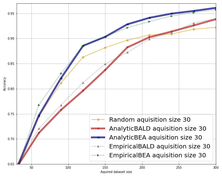
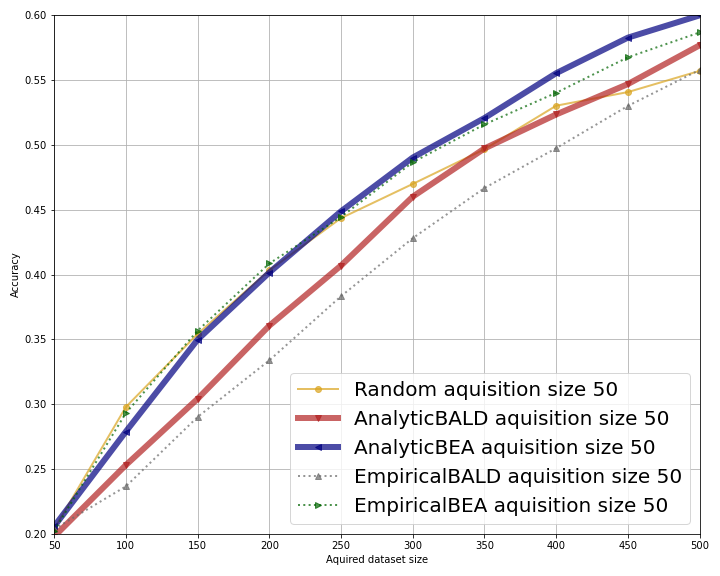
In our experiments, we use MNIST and EMINST datasets [46, 47]. MNIST is the most popular dataset to validate the performance of image-based deep learning models and the EMNIST dataset is a set of handwritten character digits aligning with the MNIST dataset. For the empirical BALD/or BEA, we apply the equation (3). For the analytic BALD/or BEA, we apply Theorem III.1.

1Input: 1) Total training dataset $\mathcal{D}_{\textbf{pool}}$, 2) randomly selected initial dataset $\mathcal{D}^{(0)}_{\textbf{training}}$, 3) $M$ as the number of dropout samples, 4) active learning budget $K$ for each iteration, 5) total active learning budget $K^{tot}$

2Initialize Bayesian neural network $\Phi$ and set $n\leftarrow 0$

3Repeat at iteration $n\geq 0$

4 Train the model $\Phi$ with $\mathcal{D}^{(n)}_{\textbf{training}}$

5 For each $\mathbf{x}\in\mathcal{D}_{\textbf{pool}}\setminus\mathcal{D}^{(n)}_{\textbf{training}}$,

6  Generate $M$ Dirichlet samples from $\Phi\left(\mathbf{x},\omega\right)$

7  Estimate Drichlet parameters $\left(\alpha_{1},\cdots,\alpha_{C}\right)$ following Minka’s fixed point iteration

8  Calculate the uncertainty value

9 Set $\mathcal{D}^{(n+1)}_{\textbf{training}}\leftarrow$ $\mathcal{D}^{(n)}_{\textbf{training}}\bigcup$ $\left\{\text{top }K\text{ uncertainty-valued }\mathbf{x}\in\mathcal{D}_{\textbf{pool}}\setminus\mathcal{D}^{(n)}_{\textbf{training}}\right\}$, and $n\leftarrow n+1$

Until $\left|\mathcal{D}^{(n-1)}_{\textbf{training}}\right|$ reaches to $K^{tot}$

Algorithm 1 Active learning algorithm

Figure 3 shows the performance of active learning results with uncertainty measures. For the MNIST dataset, we use the acquisition size $K=30$ in each iteration up to $K^{tot}=300$ number of images. For EMNIST dataset, we use the acquisition size of $K=50$ for each iteration up to $K^{tot}=500$ number of images. We start from a randomly selected initial training set for both cases to train the initial model. We note that BALD suffers from improving the accuracy compared to the random case since it cannot effectively remove the redundancy. We confirm that analytic BALD and analytic BEA show similar in MNIST or better behavior in EMNIST with empirical BALD and empirical BEA.

VII Conclusion

This paper presented analytic mutual information in Bayesian neural networks and their application in active learning. We derived the analytical formula of the mutual information as an epistemic uncertainty or the conditional entropy as an aleatoric uncertainty. Aligning with the recent success of BalEngAcq (BEA) [33], we expect that our analytical framework would enhance the understanding of BalEngAcq as well as the further applications of the Bayesian neural network to build a robust and reliable neural network model.

References

- [1] A. Kendall and Y. Gal, “What uncertainties do we need in bayesian deep learning for computer vision?” Advances in neural information processing systems, vol. 30, 2017.
- [2] H. Jiang, B. Kim, M. Y. Guan, and M. Gupta, “To trust or not to trust a classifier,” Neural Information Processing Systems, 2018.
- [3] E. Begoli, T. Bhattacharya, and D. Kusnezov, “The need for uncertainty quantification in machine-assisted medical decision making,” Nature Machine Intelligence, vol. 1, no. 1, pp. 20–23, 2019.
- [4] E. Hüllermeier and W. Waegeman, “Aleatoric and epistemic uncertainty in machine learning: An introduction to concepts and methods,” Machine Learning, vol. 110, no. 3, pp. 457–506, 2021.
- [5] R. M. Neal, Bayesian learning for neural networks. Springer Science & Business Media, 2012, vol. 118.
- [6] N. Srivastava, G. Hinton, A. Krizhevsky, I. Sutskever, and R. Salakhutdinov, “Dropout: a simple way to prevent neural networks from overfitting,” The journal of machine learning research, vol. 15, no. 1, pp. 1929–1958, 2014.
- [7] D. Barber and C. M. Bishop, “Ensemble learning in bayesian neural networks,” Nato ASI Series F Computer and Systems Sciences, vol. 168, pp. 215–238, 1998.
- [8] H. A. Chipman, E. I. George, and R. E. McCulloch, “Bayesian ensemble learning,” Advances in neural information processing systems, vol. 19, p. 265, 2007.
- [9] T. Pearce, F. Leibfried, and A. Brintrup, “Uncertainty in neural networks: Approximately bayesian ensembling,” in International conference on artificial intelligence and statistics. PMLR, 2020, pp. 234–244.
- [10] D. P. Kingma and M. Welling, “Auto-Encoding Variational Bayes,” in 2nd International Conference on Learning Representations, ICLR 2014, Banff, AB, Canada, April 14-16, 2014, Conference Track Proceedings, 2014.
- [11] Y. Gal and Z. Ghahramani, “Dropout as a bayesian approximation: Representing model uncertainty in deep learning,” in international conference on machine learning. PMLR, 2016, pp. 1050–1059.
- [12] H. Ritter, A. Botev, and D. Barber, “A scalable laplace approximation for neural networks,” in 6th International Conference on Learning Representations, ICLR 2018-Conference Track Proceedings, vol. 6. International Conference on Representation Learning, 2018.
- [13] M. Hobbhahn, A. Kristiadi, and P. Hennig, “Fast predictive uncertainty for classification with bayesian deep networks,” arXiv preprint arXiv:2003.01227, 2020.
- [14] H. G. Matthies, “Quantifying uncertainty: modern computational representation of probability and applications,” in Extreme man-made and natural hazards in dynamics of structures. Springer, 2007, pp. 105–135.
- [15] N. Houlsby, F. Huszár, Z. Ghahramani, and M. Lengyel, “Bayesian active learning for classification and preference learning,” arXiv preprint arXiv:1112.5745, 2011.
- [16] F. Baccelli and J. O. Woo, “On the entropy and mutual information of point processes,” in 2016 IEEE International Symposium on Information Theory (ISIT). IEEE, 2016, pp. 695–699.
- [17] C. K. Williams and D. Barber, “Bayesian classification with gaussian processes,” IEEE Transactions on Pattern Analysis and Machine Intelligence, vol. 20, no. 12, pp. 1342–1351, 1998.
- [18] C. Rasmussen and C. Williams, “Gaussian processes for machine learning. adaptive computation and machine learning,” 2006.
- [19] D. Milios, R. Camoriano, P. Michiardi, L. Rosasco, and M. Filippone, “Dirichlet-based gaussian processes for large-scale calibrated classification,” arXiv preprint arXiv:1805.10915, 2018.
- [20] A. Kristiadi, M. Hein, and P. Hennig, “Being bayesian, even just a bit, fixes overconfidence in relu networks,” in International Conference on Machine Learning. PMLR, 2020, pp. 5436–5446.
- [21] E. Daxberger, A. Kristiadi, A. Immer, R. Eschenhagen, M. Bauer, and P. Hennig, “Laplace redux-effortless bayesian deep learning,” Advances in Neural Information Processing Systems, vol. 34, 2021.
- [22] C. E. Shannon, “A mathematical theory of communication,” The Bell system technical journal, vol. 27, no. 3, pp. 379–423, 1948.
- [23] D. V. Lindley, “On a measure of the information provided by an experiment,” The Annals of Mathematical Statistics, pp. 986–1005, 1956.
- [24] Y. Gal, R. Islam, and Z. Ghahramani, “Deep bayesian active learning with image data,” in International Conference on Machine Learning. PMLR, 2017, pp. 1183–1192.
- [25] D. G. Tzikas, A. C. Likas, and N. P. Galatsanos, “The variational approximation for bayesian inference,” IEEE Signal Processing Magazine, vol. 25, no. 6, pp. 131–146, 2008.
- [26] A. Kirsch, J. van Amersfoort, and Y. Gal, “Batchbald: Efficient and diverse batch acquisition for deep bayesian active learning,” 2019.
- [27] J. McFadden, “The entropy of a point process,” Journal of the Society for Industrial & Applied Mathematics, vol. 13, no. 4, pp. 988–994, 1965.
- [28] J. Fritz, “An approach to the entropy of point processes,” Periodica Mathematica Hungarica, vol. 3, no. 1-2, pp. 73–83, 1973.
- [29] F. Papangelou, “On the entropy rate of stationary point processes and its discrete approximation,” Probability Theory and Related Fields, vol. 44, no. 3, pp. 191–211, 1978.
- [30] D. J. Daley and D. Vere-Jones, An introduction to the theory of point processes: volume II: general theory and structure. Springer Science & Business Media, 2007, vol. 2.
- [31] C. Nair, B. Prabhakar, and D. Shah, “On entropy for mixtures of discrete and continuous variables,” arXiv preprint cs/0607075, 2006.
- [32] D. J. MacKay, “Choice of basis for laplace approximation,” Machine learning, vol. 33, no. 1, pp. 77–86, 1998.
- [33] J. O. Woo, “Active learning in bayesian neural networks: Balanced entropy learning principle,” arXiv preprint arXiv:2105.14559, 2021.
- [34] N. Ebrahimi, E. S. Soofi, and S. Zhao, “Information measures of dirichlet distribution with applications,” Applied Stochastic Models in Business and Industry, vol. 27, no. 2, pp. 131–150, 2011.
- [35] J. Lin, “On the dirichlet distribution,” Master’s Thesis, 2016.
- [36] G. B. Folland, Real analysis: modern techniques and their applications. John Wiley & Sons, 1999, vol. 40.
- [37] F. Beukers, “Special functions (encyclopedia of mathematics and its applications 71),” Bulletin of the London Mathematical Society, vol. 33, no. 1, pp. 116–127, 2001.
- [38] T. P. Minka, “Estimating a dirichlet distribution,” Tech. Rep., 2000.
- [39] M.-F. Balcan, S. Hanneke, and J. W. Vaughan, “The true sample complexity of active learning,” Machine learning, vol. 80, no. 2, pp. 111–139, 2010.
- [40] P. Bangert, H. Moon, J. O. Woo, S. Didari, and H. Hao, “Medical image labeling via active learning is 90% effective,” in Future of Information and Communication Conference. Springer, 2022, pp. 291–310.
- [41] ——, “Active learning performance in labeling radiology images is 90% effective,” Frontiers in Radiology, p. 13.
- [42] H. Hao, H. Moon, S. Didari, J. O. Woo, and P. Bangert, “Highly efficient representation and active learning framework for imbalanced data and its application to covid-19 x-ray classification,” NeurIPS Data-Centric AI Workshop, 2021.
- [43] D. A. Cohn, Z. Ghahramani, and M. I. Jordan, “Active learning with statistical models,” Journal of artificial intelligence research, vol. 4, pp. 129–145, 1996.
- [44] B. Settles, “Active learning literature survey,” 2009.
- [45] C. C. Aggarwal, X. Kong, Q. Gu, J. Han, and S. Y. Philip, “Active learning: A survey,” in Data Classification. Chapman and Hall/CRC, 2014, pp. 599–634.
- [46] Y. LeCun and C. Cortes, “MNIST handwritten digit database,” 2010. [Online]. Available: http://yann.lecun.com/exdb/mnist/
- [47] G. Cohen, S. Afshar, J. Tapson, and A. Van Schaik, “Emnist: Extending mnist to handwritten letters,” in 2017 International Joint Conference on Neural Networks (IJCNN). IEEE, 2017, pp. 2921–2926.