Natural Selection and Random Matrix Theory
Mehdi Ameri

Ferdowsi University of Mashhad
Faculity of Science, Physics Department

We will study the relation between two well-known theories, genetic evolution and random matrix theory in the context of many-body systems and chaos theory. We show that the time evolution of certain chaotic quantum mechanical models is similar to the evolution of a living cell. It is also suggested that natural selection can be described by a random matrix theory with statistical distribution in which the genetic evolution acts as a Gross-Witten-Wadia phase transition.

1 Introduction

It is amazing if we look at different branches of science, we would find out they are originated from the same root. So besides the advanced studies in a single area, one has to study other branches as well, seeking connections. One of these branches that can be directly related to quantum physics is the genetics and the biology of living cells. We aim our focus to the well-known concept in genetic science called Evolution. Evolution theory was first proposed by Charles Darwin in 1859 [1] and then it was significantly modified to the new version by Mendel [2, 3, 4].

It is strongly believed that all species on earth are evaluated from a complex single-celled organism called Last Universal Common Ancestor (LUCA). From the Darwinism point of view, this theory proposes that all the living beings are evaluated from each other since the creation of the first living cell or the ancestor. Darwin also said that human beings are the result of the evolution of four-legged mammals like chimpanzees regarded as Homo Sapiens, however, this may be in contrast with the new version of evolution. The newest version proposes a completely different viewpoint in which it contains three different ancestors: (1) Bacteria, (2) bacteria-like microbes (Archaea), and (3) Eukaryotes, the group that includes plants and other species, such as animals and humans. All three cases are independent of each other, and it is also believed that today’s human life may be evaluated from a completely different cell than from other animals. Plants and trees cells contain certain organic materials like chlorophyll which is responsible to transform the sunlight into organic nutritional products whereas animals and humans cells contain more complex structures.
The evolution works in the direction of modifying the mechanism of the entire physical living system to a new more advanced system to protect the living being from external intense conditions. When a creature undergoes unexpected natural stresses and anomalies, the natural selection would evaluate it to a more stable version to have the needed defense and the protection against the unwilling behaviors. Evolution is a very long-term process and its time scales with millions of years. That is why the observations of fossils of dinosaurs and other ancient remnants can be surprisingly beneficial. The evolution is strongly correlated with external environmental conditions such as air pressure, temperature, food resources, cosmic rays, etc. and it also depends on the occurrence of natural disasters like earthquakes, asteroids, hurricanes, etc.
The basic question one can ask is that on what scale does the evolution happen? Yet, the answer is ambiguous and it is mostly considered in cellular scales. In this paper, we want to discuss the subject on a special scale where the quantum dynamic is dominant and all the dynamic is represented by probability laws. It has been observed that cosmic rays can remarkably affect evolution and it would be strange to see the existence of life is in hands of probabilities. This also means that there is a state in which our existence may not have occurred at all! If the evolution happens in a quantum mechanical way, then its dynamics can be described by the space of possible states or Hilbert space which contains finite possible states to be observed by the observer. The observed states are our observables in daily life but this does not mean that the other states do not exist. This is due to the fundamental uncertainty principle of quantum mechanics.
This whole scenario is meanly pointing out that natural selection can occur quantum mechanically and choose between an infinite number of possible states with random distribution each with a specific probability weight. This is known as Quantum Darwinism and first proposed by [5].
Consider a setup like fig. (1) where we are trying to observe the actual spin of the electron beam. The spin is an intrinsic quantity of a particle that determines the magnetic field of the particle and its magnetic interaction with other particles with the same type of spin.
If the observer detects the z component at first then changes the setup to measure another component like x, the former spin result will be completely changed. If we measure the z component again it may give us a completely different value. This is unexpected because spin is an intrinsic property. So we conclude that the effects of the observer $SG_{x}$ have changed the history of the particle.

Figure 1: Stern-Gerlach setups to determine each spatial component of the spin. This shows that the contribution of $SG_{x}$ has cleaned the history of the particle and at the end, both $z$ component appears. This is strange since we are blocked $S_{z^{-}}$ in the first measurement. This directly leads to the principle that one can not exactly measure two quantities of the quantum system at the same time. Once we try to do so, the system will be disrupted.

Having said that the states of the system can be chosen accidentally with a specific probability weight, so the evolution from one level to an upper advanced level can also be picked up randomly. This is possible if we assume that the early evolution series has happened quantum mechanically. However, random matrix theory is also can be used for classical phenomena as well.
Random matrix theory describes many-body chaotic systems with strong coupling between its partitions which are basically thermal systems and it has been intended to study statistical behaviors. The random matrix theory is used in various fields, such as string theory, two-dimensional gravity [6], conformal field theory, number theory, condensed matter [7], integrable systems, glass theory, [8], and stochastic processes [9]. This theory is also the basis of many scientific applications of economics [10]. Moreover, a big development of this theory has been made and specified to study the RNA folding [11, 12, 13, 14, 15, 16, 17]. It is quite wondering that the natural selection can be completely random and more wondering is that this randomness can be exactly analyzed and by choosing an appropriate distribution for matrix elements, one can see on what conditions the genetic evolution takes place which can also be checked in the laboratory.
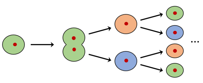
The state of the living cell before the decomposition can be considered as a random matrix and when the decomposition starts it will generate two other random matrices between $m$ possible set of states (fig. (2)). This is what we call in this paper natural selection and it does not always lead to an evolutionary change in the DNA structure. Just if the environmental conditions change intensely the decoupling may get a genetic disorder after the decomposition as we expect from a strongly coupled chaotic system (see sec.(2),(3)).
Another point is that if we write each state growth as a random matrix model with matrices of size $L$ and the coupling constant $g$, then at the double scaling limit ($L\rightarrow\infty$ and $g\rightarrow g_{c}$), each state construct a group of manifolds with $h$ handles and $n$ boundaries [6]. Therefore, all $m$ states can be considered as the moduli space of Riemann surfaces and one can find an appropriate $SL(2,\mathbb{R})$ transformation between every two states [18, 21, 22, 23]. One can also be able to find Eynard-Orantin [24, 25, 26, 27] or Mirzakhani’s recursion relation [18, 19, 20] between the manifolds of each state.

Figure 2: If the mechanism of decomposition of the living cell is assumed quantum mechanically then there are $m$ possible states for the cell to choose. Each has its growth and probability weight. In the next sections, we explain that the states $1,2,...,m$ can be represented by a random matrix theory.

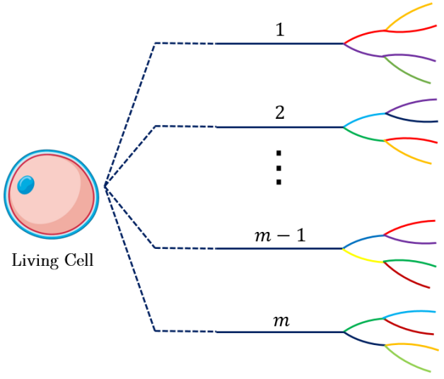
The context of evolution is related to several scientific approaches. Since it is very sensitive to initial environmental and internal conditions, it can be considered as a system with chaotic behavior and can be studied in the context of chaos theory. In section (2), we will give a general view of the chaos theory and see how such systems can be mathematically analyzed and related to quantum mechanics.

In section (3), we show that the exponential evolution of a quantum chaotic system is similar to the exponential growth of bacterial or cellular binary fission.

In section (4), First, we give a general view of the DNA’s structure and discuss the probability of $n$ possible evolutions that can happen between $m$ states of the cell proliferation. Moreover, we will point out an important idea that can explain natural selection as a phase transition in the large $L$ random matrix theory.

Finally, Remarks and conclusions will be given in section (5) to sum up the discussions argued in this paper.

2 Chaos Theory

Chaos in specific systems is known as a periodic long-time behavior that is very sensitive to initial conditions. Many physical systems follow this kind of behavior and chaos is a universal feature. A system with a strong correlation between its partitions, with a small variation on its physical quantities, can be significantly changed to a different state in a long time. A famous example is that if a hurricane is occurring at a specific time in one region of the earth, flying a butterfly close to that region can evaluate the system drastically. This evolution may cause a bigger hurricane in the northern regions of the earth. This is known as the butterfly effect. These systems are chaotic and predicting their evolution over time is a hard piece of work. However, sometimes chaotic behavior of small partitions of a system on a large scale and long times can lead to an equilibrium that is well-defined without any erratic behavior. For example, a very hot gas into a box in microscopic scale and short times may seem quite complicated to study but on the other hand, from the statistical point of view, In macroscopic scales and long times, the system ends up with an equilibrium state and completely predictable. Although studying chaotic systems seem to be intense, physics and mathematical developments have accomplished great progress in this background. one of these developments is studying their energy spectrum. The energy spectrum of chaotic systems is completely different from integrable systems in which one has to use nonperturbative statistic models to investigate their features. One of the best of these models is the Random Matrix Theory (RMT) [46, 47, 48, 49].

In this section, we first present an overview of chaos theory in classical and quantum mechanical contexts and then connect the subject with bacterial growth. Generally, most multi-particle quantum systems with strong coupling constants are chaotic. Consider a particle in phase space, at time zero in point $q(0)$ with momentum $p(0)$ which travels with a specific velocity on an arbitrary path. Now if at time zero, we make small variations $(\delta p(0))$ and $(\delta q(0))$ on particle’s momentum and position, these variations will grow exponentially with time and the particle will take a completely different path because of the sensitivity of the system on initial conditions (figure b of (3)).

$$\frac{\delta q(t)}{\delta q(0)}=Ce^{\lambda_{L}t}\,$$ (2.1)

Where $\lambda_{L}$ is called the Lyapunov exponent and $C$ is a constant value. By replacing the derivative with the variations, the left-hand side of (2.1) would be equal to a Poisson bracket

$$\frac{\delta x(t)}{\delta x(0)}=\{x(t),p(0)\}=Ce^{\lambda_{L}t}\,$$ (2.2)

For some reason, a direct modification of chaos to quantum systems is not available [28].

Figure 3: (a) By producing very small variations on initial conditions, these variations will grow over time. If the system is integrable (blue trajectories), small variations in initial conditions will lead to a slightly different path with a little difference from the first one and in some cases is neglectable. These paths are stable and diverge with a linear combination of time. In a chaotic system (red trajectories), small variations will lead to a very big difference in the future of particles and the particle would travel on a completely different path. These paths are unstable and diverge exponentially with time. (b) The ratio of the particle path in second zero $(\delta q(0))$ to the difference in the same path in second $t$, $(\delta q(t))$, grows exponentially with time (equation(2.1)).

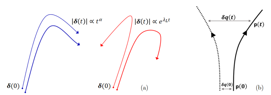
Larkin and Ovchinnikov provided an intuitive definition of chaos in the semi-classical regime [31]. To modify the problem to quantum systems we just need to use operator commutation relation instead of Poisson bracket. Generally, the commutator is an operator, so for observing the exponential growth we need to calculate the expectation value of the commutator. The expectation value of the commutator in the thermal state becomes zero due to phase cancelation. A simple way to fix this is to consider the square of the commutator [31],

$$\langle[x(t),p(0)]^{2}\rangle_{\beta}=C^{2}\hbar^{2}e^{2\lambda_{L}t}\,.$$ (2.4)

The expectation value of the commutator saturates to a maximum value (fig.(4)) at a specific time which is called the scrambling time.

Figure 4: The commutation grows exponentially and in a specific time $t_{*}$, the growth will saturate.

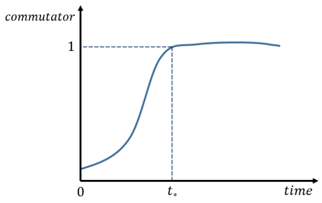
In the context of black hole physics, this is how long it takes for the information to be spread on the area which is logarithmic in terms of the total number of degrees of freedom of the system. For example, if an electron goes toward the black hole’s horizon from a certain radius, by considering a conductive surface for the horizon, the amount of time it takes for the electron’s charge density to be scattered on the horizon’s area is of order the scrambling time [29]. If we throw a diary toward the black hole, the amount of time we have to wait for the first information to reach us in the form of Hawking radiation (after Page’s time) is also equal to the scrambling time [30].
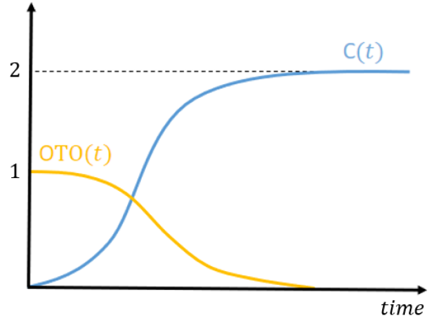
Equation (2.4) includes a set of four-point functions that are known as Out-of-Time Order correlation functions (OTO). A key point is that in a chaotic system, the behavior of $OTO(t)$ functions is exponential with time. Consider the following four-point function:

$$OTO(t)\equiv\langle\psi|W(t)V(0)W(t)V(0)|\psi\rangle\,$$ (2.5)

Where $V(0)$ and $W(t)$ are two hermitian operators $(WW^{\dagger}=W^{2}=1,VV^{\dagger}=V^{2}=1)$ in time zero and $t$. Now we define the function $C(t)$:

$$C(t)\equiv\langle\psi|-[W(t),V(0)]^{2}|\psi\rangle=\langle\psi|W(t)V(0)V(0)W(T)+V(0)W(t)W(t)V(t)-$$

$$-W(t)V(0)W(t)V(0)-V(0)W(t)V(0)W(t)|\psi\rangle=2[1-Re(OTO)]\,$$ (2.6)

Where $OTO(t)$ and $C(t)$ parts evaluate with time as shown in figure (5). Sometimes it is more convenient to work with $C(t)$ instead of using $OTO(t)$ directly. The reason behind the decaying of $OTO(t)$ function is that if firstly we affect the operator $V(0)$ and $W(t)$ on the state of the system, because of the sensitivity on the initial conditions, the state of the system becomes completely indistinguishable from the previous one in time $t$. Consequently, if operators $V(0)$ and $W(t)$ act again on the state of the system, The correlation between the primary state and the secondary state decreases over time.

Figure 5: The behavior of OTO(t) and C(t) functions with time.

Now to estimate time $t_{*}$, We will consider a specific system with $N$ particles, with the following interactive Hamiltonian

$$H=\frac{1}{3!}\sum\limits_{i<j<k}^{N}\gamma_{ijk}S_{i}S_{j}S_{k}\,,$$ (2.7)

Where $S$ are spinor operators which can evaluate with time and interact with other particles. The parameter $\gamma_{ijk}$ is a matrix picked randomly, so (2.7) is an ensemble of Hamiltonians. The model with four-interactive spins is deeply analyzed and it is called the Sachdev-Ye-Kitaev model [32, 33, 34].
If we let one spin operator evaluates with time, by using the Baker-Hausdorff lemma we can write

$$S_{j}(t)=e^{iHt}S(0)e^{-iHt}=\sum\limits_{k=0}^{\infty}\frac{(it)^{k}}{k!}[H,[H,...,[H,S_{j}]]]\,,$$ (2.8)

Where $t$ is time and $k$ is the order of expansion and the number of Hamiltonian commutations with $S_{j}$. According to figure (6) in every order of time, by commutating the operator $S_{j}$ with the Hamiltonian (2.7), the particle first interacts with the other two particles, then with the other four, and this rate will grow with time.

Figure 6: The commutation of the spin with Hamiltonian in each time step, based on equation (2.8), the spin interacts with two particles (or decay to two particles) and this behavior will grow exponentially with time until it interacts with the Nth particle of the system in $t_{*}$.

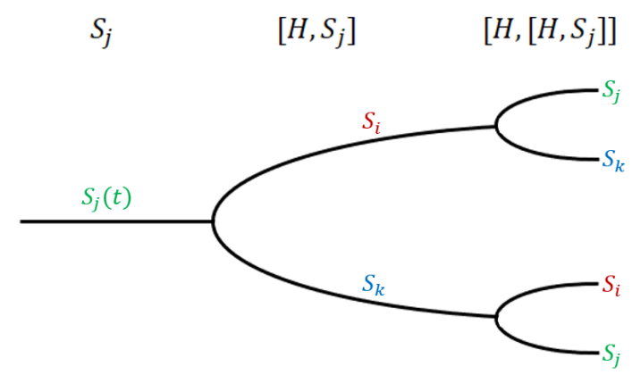
Note that in each step there are a bunch of spinor matrices that are random and independent due to the choice of $\gamma_{ijk}$. Since $\gamma_{ijk}$ depends on the orders of indices and the Hilbert space dimension $2^{N/2}$, this growth will stop at the scrambling time. Although $S_{i}$ and $S_{j}$ will form in the first place, $S_{j}$ can be reproduced with different random distributions after some steps.
If we consider the system is compact on a circle or a sphere and all particles have the same distance from each other, the question one may ask is that when the particle $S_{j}$ will interact with (or decay to) the $N$th particle? In other words, how long does take for the information to be spread on the entire system? It is clear from figure (6) that the operator growth is exponential and the time should be equivalent to the logarithm of the number of particles in base two for each temporal step. Therefore for a thermal system with chaotic evolution, this time would be

$$t_{*}=c\beta log_{2}(N/N_{0})=c\beta log_{2}(S)\,,$$ (2.9)

Where $N$ is the total number of particles that directly determine the entropy ($N\sim S$). $\beta$ is the inverse of temperature which is added to maintain the dimension of time and $c$ is a proportionality constant factor. This behavior in $k$ temporal steps is also referred to as k-locality or operator growth.

Maldacena, Shenker, and Stanford have shown that for every quantum chaotic system, the Lyapunov exponent can not exceed a maximum value. This value is called the chaos bound or Maldacena-Shenker-Stanford (MSS) bound and it is given by [38],

$$\lambda_{L}\leq\frac{2\pi k_{B}T}{\hbar}\,,$$ (2.10)

Where $T$ is the temperature of the system. The classical limit of this equation occurs when we take $\hbar\rightarrow 0$ and this means that classical chaotic systems have no limit on the Lyapunov exponent. Now by taking $k_{B}$=$\hbar$=1, the chaos bound becomes

$$\lambda_{L}\leq\frac{2\pi}{\beta}\,.$$ (2.11)

For a Schwarzschild black hole, it has been shown that the energy spectrum near the horizon is chaotic and $\lambda_{L}$ is equal to the surface gravity parameter $\kappa$ which is given by

$$\lambda_{L}=\kappa=\frac{2\pi}{\beta}\,.$$ (2.12)

For Shwartzchild black hole $\kappa=\frac{1}{4MG}$ and by substituting it in equation (2.12) we would obtain Hawking temperature [35]. For $OTO(t)$ and $t_{*}$ we have

$$OTO(t)\propto\frac{1}{S}e^{\kappa t}\,,~{}~{}~{}~{}~{}~{}t_{*}=\frac{\beta}{2\pi}ln(S)\,.$$ (2.13)

Therefore the constant $c$ in equation (2.9) is equal to $\frac{1}{2\pi}$. Here $S$ is the black hole entropy [35, 36, 37]. In conclusion, black holes saturate the chaos bound which means black holes are one of the most chaotic quantum systems known. That is why these systems are sometimes called fast scramblers. This has been conjectured by Sekino and Susskind [39] and then proved in [40, 41, 42, 43, 44, 45].
In the next section, we will see that this behavior also appears in the case of bacterial or cellular proliferation, which motivates us toward using this natural decomposition as a single choice of many choices on an ensemble.

3 Bacterial and Cellular Proliferation

In this section, we will consider binary fission with initial $N_{0}$ numbers of bacterias. After $k$ generations the total number of bacteria would be equal to $N$. This can be given by

$$\frac{N}{N_{0}}=2^{k}\,,$$ (3.1)

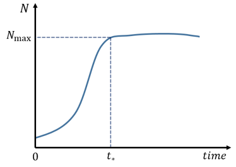
We will conventionally take $N_{0}=1$. In each generation, the number of bacteria doubles until it gets the maximum total number $N_{max}$ (fig. (7)).

Figure 7: Bacterial or cellular binary proliferation. The mechanism is similar to what happens in fig. (6). Each color corresponds to a different random matrix.

The exponential growth phase will turn into the stationary phase at the scrambling time (fig.(8)):

$$t_{*}=\alpha\beta log_{2}(N_{max})\,,$$ (3.2)

Where $\alpha$ is a constant of proportionality and can be experimentally determined by the data of bacterial growth. This is reasonable since the stationary phase is proportional to the total number of bacteria $N_{max}$. Note that in the stationary phase, the amount of produced bacterias is roughly the same as those who are dying and the overall number remains fixed. Moreover, we know that as the temperature increase, the growth rate of the organism is also increased and that is clear from fig. (8) in which the scrambling time gets shorter when the temperature gets higher. However one has to be careful about the amount of the temperature since in very high temperatures the growth can be drastically drop down and this shows the side detrimental effects on the living system.

Figure 8: The bacterial growth has an exponential behavior in log phase and it will stop at the scrambling time $t$ and turn to the stationary phase. A similar process happens in fig.(4). Note that we are did not consider the death phase here.

The Lyapunov exponent hence can be written as:

$$\lambda_{L}=\frac{\text{total number of generations}}{\text{scrambling time}}=\frac{k_{total}}{t_{*}}=\frac{k_{total}}{\alpha\beta log_{2}(N_{max})}\,,$$ (3.3)

The genetics of the bacteria may change in each step and produce different kinds of bacteria through changing the genetic codes. This is not a stable phenomenon and can reproduce early bacterias again in the next generations (fig. (7)) which is also applied for the cells. This exponential growth was one feature of the systems that were described by random matrix theory similar to what is discussed in section (2), however, in the next section, we will give another perspective that shows a genetic deformation can occur randomly at each generation step through DNA reconstruction in the decomposition process.

4 Random Matrix Theory and Evolution

Random matrix theory is a strong mathematical tool to study the statistical behavior of chaotic systems such as the heavy nucleus, black holes, hurricanes, or here a system like DNA. It has been beautifully developed for physics applications by Wigner and Dyson and then by many other people like Gaudin and Mehta. For useful reviews on this context see [46, 47, 48, 49].

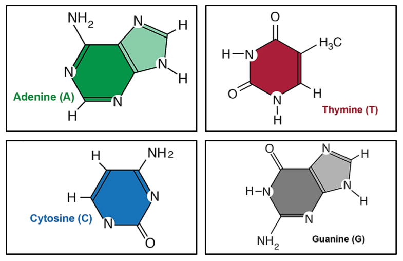
A single DNA is constructed of two sugar phosphate backbones and four nucleotides namely Adenine (A), Thymine (T), Cytosine (C), and Guanine (G) (fig. (9) and (10)). If each bond between A, T, C, and G codes on a DNA represent a force with a random value on a specific distribution with zero mean and determined variance $\mathcal{V}$, the total DNA would make a huge random matrix of the size of the DNA in terms of the A, T, C and G bonds which can be changed randomly in each generation step. The force can be determined by the potential energy ($F=-\nabla U$) therefore each covalent bond carries a specific amount of energy and hence one can write the random matrix on an energy basis and find the energy eigenvalues of each cell’s DNA by diagonalization of the matrix. The codes have correlations among each other and that is in common with the feature of the correlation between eigenvalues in the random matrix theory.

Figure 9: Chemical structure of the fundamental nucleotides.

In the decomposition of the cell, the DNA will separate into two branches to construct two other cells from the same gene. In the whole process, the matrix elements will change randomly, each bond in a specific variance, and that will lead to different matrices for both produced cells. The random matrix would choose one of the $m$ possible states (see fig. (2)) to start the reproduction process randomly. Each state has its probability weight and the one which has greater probability is more likely to be naturaly selected.
If each state grows with $k_{i}$ generation where $i=1,...,m$ and each produce $N_{max}^{(i)}=2^{k_{i}}$ particles at the scrambling time $t_{*}^{(i)}$, than the probabilty of having $n$ genetic evolution is equal to:

$$P_{n}=\frac{n}{N_{max}^{(1)}+N_{max}^{(2)}+...+N_{max}^{(m)}}=\frac{n}{\sum_{i=1}^{m}2^{k_{i}}}$$ (4.1)

For example if we consider all states have the same number of generations $k_{i}=k=\frac{t_{*}}{\alpha\beta}$ therefore for n=1:

$$P_{1}=\frac{2^{-\gamma T}}{m}$$ (4.2)

where we denoted $\gamma=\frac{t_{*}}{\alpha}$ and replaced $\beta=\frac{1}{T}$. In $T\rightarrow\infty$ limit the probability is simply zero since in high temperatures the cell will no longer can still alive to be prepared for evolution. In the $T\rightarrow 0$ limit, the cell can not be evaluated to multiple partitions and it will be stuck on the first stage hence the probability only depends on the number of states $m$, i.e. $P=\frac{1}{m}$.

Figure 10: The structure of DNA (right) and the nucleotide bindings (left).

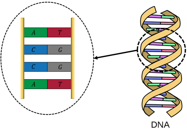
In DNA, the energy can differ from one bond to another. For example, an AT bond on one part of the DNA can have slightly different energy than the AT bond on the other part. That is possible since this energy depends on the location of the nucleotides and the side effects of the potentials of other objects. By seeing this bond energy as a random variable, the DNA can have statistical distribution in terms of energy eigenvalues, and hence each DNA can be seen as a $2\times L$ random matrix M (also see [50]):

$$M=\begin{pmatrix}E_{AT}^{(1)}&E_{GC}^{(1)}\\[5.69046pt] E_{AT}^{(2)}&E_{GC}^{(2)}\\[5.69046pt] \vdots&\vdots\\[5.69046pt] E_{AT}^{(L)}&E_{GC}^{(L)}\\ \end{pmatrix}$$ (4.3)

Where $L$ is the length of the DNA, the size of the random matrix, and the total number of bindings. $E_{AT}$ and $E_{GC}$ are the Energy of A-T and G-C bindings respectively. For example, If the length of DNA is $L=4$ as the case of fig. (10), this matrix would be:

$$M=\begin{pmatrix}E_{AT}^{(1)}&0\\[5.69046pt] 0&E_{GC}^{(2)}\\[5.69046pt] 0&E_{GC}^{(3)}\\[5.69046pt] E_{AT}^{(4)}&0\\ \end{pmatrix}$$ (4.4)

One chromosome is built out of two random matrix DNAs and can be defined as:

$$C\equiv M.\widetilde{M}=\begin{pmatrix}E_{AT}^{(1)}&E_{GC}^{(1)}\\[5.69046pt] E_{AT}^{(2)}&E_{GC}^{(2)}\\[5.69046pt] \vdots&\vdots\\[5.69046pt] E_{AT}^{(L)}&E_{GC}^{(L)}\\ \end{pmatrix}\begin{pmatrix}\widetilde{E}_{AT}^{(1)}&\widetilde{E}_{AT}^{(2)}&\cdots&\widetilde{E}_{AT}^{(L)}\\[5.69046pt] \widetilde{E}_{GC}^{(1)}&\widetilde{E}_{GC}^{(2)}&\cdots&\widetilde{E}_{GC}^{(L)}\\ \end{pmatrix}=\sum_{i=1}^{L}\begin{pmatrix}E_{AT}^{(i)}.\widetilde{E}_{AT}^{(i)}&E_{GC}^{(i)}.\widetilde{E}_{AT}^{(i)}\\[5.69046pt] E_{AT}^{(i)}.\widetilde{E}_{GC}^{(i)}&E_{GC}^{(i)}.\widetilde{E}_{GC}^{(i)}\\ \end{pmatrix}$$ (4.5)

This is a $2\times 2$ random matrix and its elements change slightly in each generation step. The off-diagonal elements can be seen as the interaction between A-T and G-C bonds in two DNAs. At the moment of decomposition process, one specific bond should not necessarily have the exact value of previous energy . We assume that the amount of energy of each bond $E_{AT}$ and $E_{GC}$ can not exceed a minimum and a maximum limit. If so the binding would lead to the destruction of one part of the DNA.
The main question of this paper is when the genetic evolution occurs in the decomposition process in this theory? Before to start answering this question, let us see when evolution happens from a biological point of view. When the cell starts to decouple two individual cells, most of the time it will preserve the original gene. The story becomes interesting when one nucleotide (like A) exchanges with another nucleotide (like C) and causes a crisis that changes the features of the living cell. This is what is referred to as genetic evolution. Now the change $A\rightarrow C$ or $T\rightarrow G$ can generate a drastic gap in the energy spectrum of the chromosome. This means one eigenvalue has changed the statistics of the chosen random matrix theory which can slightly deviate the shape of the density of eigenvalues distribution function.
This evolution can be related to the phase transition concept in random matrix theory since it also describes a great variation on a random system through the distribution near the maximum eigenvalue. This has been widely studied and we are not going to go through the complete details in this paper. This phase transition should depend on the external environmental effects near the cell’s DNA.
Robert May has argued in [51] that a random complex interacting system will remain stable if the largest eigenvalue of the distribution is less than an inverse of the coupling constant of the system $g$:

$$\lambda_{max}<(g)^{-1}$$ (4.6)

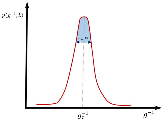
Hence there is a critical value for $g$ in which on that point the system would experience a phase transition. The probability distribution and its derivative are depicted in fig. (11) and (12) where the solid lines are for a low finite $L$ and the dashed line for large $L$. We are interested in a large finite $L$ case where the phase transition can occur on a gap of order $L^{-2/3}$. The probability distribution of the hill in the gap region is purely Gaussian however the tails connected to that hill from the left and right sides are not quite Gaussian and they are given by certain functions that satisfy the Painlevé $II$ equations. These functions of the tails and the probability density of the gap near $g_{c}$ have been well-studied by Craig Tracy and Harold Widom [52, 53, 54]. This development is called Tracy-Widom distribution and has plenty of useful practical applications.

Figure 11: The probability of having $\lambda_{max}<(g)^{-1}$ between $L$ eigenvalues in terms of $g^{-1}$. The three solid lines are for small $L$ and the dashed line is for large but finite $L$. There is a critical value for $g$ where the continuous phase transition can occur from the unstable (red line) to the stable (green line) phase. For large $L$, there is a small central region near $g_{c}^{-1}$ with a width of order $L^{-2/3}$ where the Tracy-Widom distribution applies.

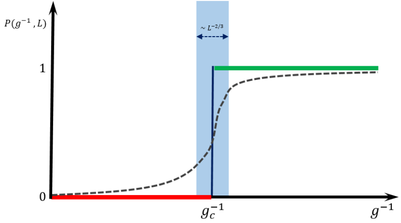
A similar phase transition occurs in two-dimensional large-$L$ lattice gauge theories in critical coupling constant which is known as Gross-Witten-Wadia (GWW) phase transition [55, 56]. In this case, the stable phase is the strong coupling phase and the unstable phase is the weak coupling phase of Yang-Mills gauge theory and the Tracy-Widom is the crossover function between these two areas in the double scaling limit (for finite but large $L$).

Figure 12: The derivative of $P(g^{-1},L)$ or the probability density function gives us the form of a delta function with a narrow Gaussian gap around the critical value. The left and right tails connected to the Gaussian Tracy-Widom distribution are described by two different functions.

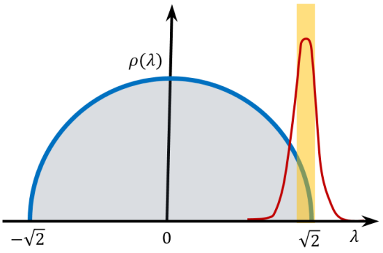
Just like many natural phenomena, if we assume the distribution of the energy bindings in a DNA has a Gaussian distribution, then the density of energy eigenvalues for large $L$ can be given by the famous Wigner semi-circle law (fig. (13)):

$$\rho(\lambda)=\frac{1}{\pi}\sqrt{2-\lambda^{2}}$$ (4.7)

The Tracy-Widom distribution apply near the edge of this semi-circle .i.e. $\sqrt{2}$. In random matrix theory, there is a Colomb force between eigenvalues in each sample. This force can differ by changing the coupling constant of the theory and that will cause a slight deviation to the effective potential where the eigenvalues condensated and therefore $g^{-1}$ can be seen as a potential well where we can move it on the real axis line of the energy. When the potential well is located out of the semi-circle (fig. (a) of (14)), no phase transition will appear. Just as the potential hit the edge of the semi-circle, it can affect the edge and change the Wigner distribution to the Tracy-Widom distribution close to that region (fig. (b) of (14)):

$$\rho^{*}_{s}(\lambda)=\frac{\sqrt{\lambda+L(s)}}{2\pi\sqrt{s-\lambda}}(s+L(s)-2\lambda),~{}~{}~{}~{}L(s)=\frac{2\sqrt{s^{2}+6}-s}{3},~{}~{}\text{where}~{}s=g^{-1}$$ (4.8)

that causes a 3rd order phase transition from stable to an unstable regime or vice versa.

Figure 13: Wigner semi-circle law for density of eigenvalues (blue curve). The red curve shows the Tracy-Widom distribution near the edge which is a perturbation around the critical value.

Figure 14: (a) Far away from the edge, the potential well does not affect the distribution and there would be no phase transition. (b) As the coupling changes, the potential will hit the semi-circle and cause a phase transition to a different distribution.

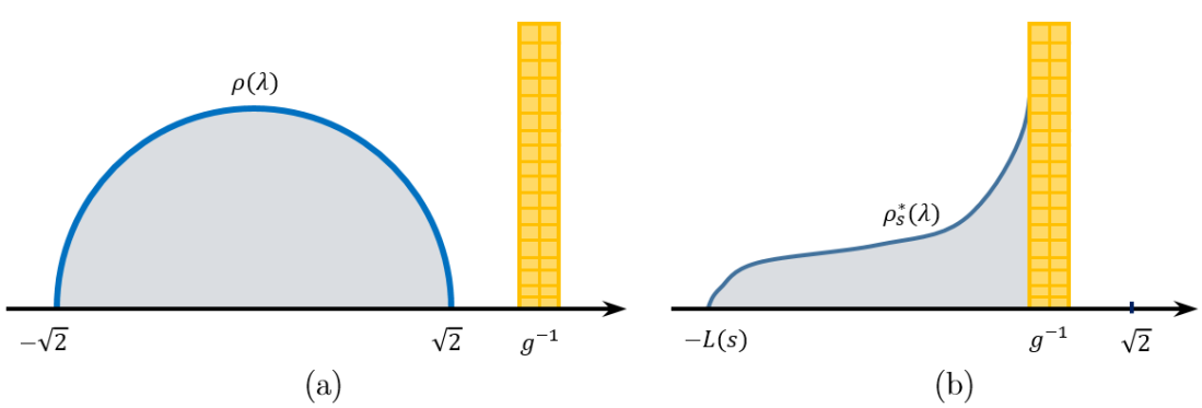
Now we turn to our former case which was the DNA random matrix. When the cell decouples in several steps, the structure of DNA may encounter some disorders from outlandish unwilling effects that put the life of the cell in danger of extinction. Therefore, the nucleotides will encounter such instabilities and decide to leave a stronger structure on the next steps of decouplings. Hence one of the nucleotides, say A, exchanges with other nucleotides which provide more powerful binding, and case the DNA will turn into the stable regime. The coupling constant does not always change in that system just if the system undergoes certain circumstances and tries to preserve its existence. Since there is an obvious interaction between nucleotides, this change transforms the coupling constant to a new value which just at the transition phase it reaches its critical value.
Statistically, if the number of energy bindings of A-T and G-C is equal (but assuming $E_{GC}>E_{AT}$), changing $A\rightarrow C$ will change the distribution from the equilibrium point. Therefore, the interaction between A-T and G-C will turn into a new regime with a less effective coupling constant between molecules. That means the larger the population of G-C can get, the more easer and more accessible it can interact with neighboring eigenvalues. Therefore, when the coupling constant gets smaller, $g^{-1}$ gets bigger and the potential well will move out of the main Gaussian distribution. One can expect that the energy cost of the potential well to get out of the semi-circle density is equal to the energy of exchanging A with C. This is similar to the Gross-Witten-Wadia phase transition from strong coupling to weak coupling regime which can turn the DNA into a more stable regime.
Since this phase transition occurs randomly in the decoupling process, it is somehow equivalent to the natural selection:

$$\text{Natural Selection}\equiv\text{GWW Phase Transition}$$ (4.9)

This phase transition can change the distribution for a short time and then keep the primary form of the distribution invariant. GWW phase transition leads to a change in specific energy eigenvalue which must be preserved in the whole process. The change in one energy eigenvalue (which has to do with the side effects such as temperature, pressure, high energy rays, etc) directly changes the other eigenvalues due to the repulsion force between every two eigenvalues.
In the next section, we will give a summary of what has been presented in this paper and mention key remarks that can be discussed in this context.

5 Conclusion and Remarks

We have given a general look at the time evolution of the random matrix spin operator and saw that this evolution is similar to the binary bacterial or cellular growth where each cell represents a Gaussian random matrix with zero mean and specific variance value. This is one state that has been selected from many other possible states. Each cell has many states to choose and evaluate, so there are an infinite number of such states, each with its probability weight. Environmental parameters such as temperature can play role in the probability value. We can conclude that the behavior of the cell is a random chaotic phenomenon that can be described in classical and quantum mechanical viewpoints by random matrix theory. Through the idea that has been presented here, one can probe the exact statistical parameters of the cell for a long period and that is possible thanks to Tracy-Widom distribution. The change in DNA bindings can directly change the overall coupling constant which leads to a GWW phase transition from unstable to the stable regime and vice versa.
One of the key points argued in this paper is that in the double scaling limit, the matrix theory diagrams can characterize a Riemann surface for DNA and one can find out what is the interpretation of phase transition in the algebraic topology. It is of significant importance to calculate the free energy of DNA in large $L$ so that it can be compared with the free energy obtained for strings scattering amplitude corresponding to planar and non-planar diagrams [58].
The GWW phase transition has been observed in the lab by laser experiments and that can open a new window to observe and keep track of the variation of DNA’s structure.
Studying the ecological treasures and connecting the effects and mechanisms inside the cell to the mathematical developments of the random matrix theory, can take a great step in tracking the number of lost circles in nature and drawing a historical map of different evolutions. By analyzing the spectrum and calculating the energy change in GWW phase transition one expects to see in what exact statistical circumstances the cells are more likely to survive.
Although the random matrix theory has been used in studying many biological applications, it can also guide us to answer fundamental questions with the help of observations.

References

- [1] C. Darwin, “On the Origin of Species”, (1859).
- [2] G. Mendel, “Experiments in a Monastery Garden”, Integrative and Comparative Biology, volume 26, issue 3 (1986), DOI: 10.1093/icb/26.3.749.
- [3] G. Mendel, “Versuche über Pflanzen-Hybriden”, Theoretical and Applied Genetics, volume 13, issue 10-11 (1941), DOI: 10.1007/bf01804628.
- [4] G. Mendel, “Versuche über Pflanzenhybriden”, Vieweg+Teubner Verlag, (1970), DOI: 10.1007/978-3-663-19714-0.
- [5] W. H. Zurek, “Quantum Darwinism”, (2009), arXiv:0903.5082.
- [6] P. Di Francesco, P. Ginsparg and J. Zinn-Justin, “2D Gravity and Random Matrices”, (1993), arXiv:hep-th/9306153v2.
- [7] C. W. J. Beenakker, “Random-matrix theory of quantum transport,” Rev. Mod. Phys. 69 731 (1997), arXiv:cond-mat/9612179.
- [8] L. F. Cugliandolo, J. Kurchan, G. Parisi and F. Ritort, “Matrix models as solvable glass models,” Phys. Rev. Lett. 74 1012 (1995), arXiv:cond-mat/9407086.
- [9] “Stochastic Processes and Random Matrices, Lecture Notes of the Les Houches Summer School,” Volume 104, July 2015, ed. by G. Schehr, A. Altland, Y. V. Fyodorov, N. O’Connell, and L. F. Cugliandolo (Oxford University Press, 2017).
- [10] J.P. Bouchaud and M. Potters, “Theory of finance risks: from statistical physics to risk management”.
- [11] H. Orland and A. Zee, “RNA Folding and Large N Matrix Theory,” Nucl. Phys. B 620 (2002), arXiv:cond-mat/0106359.
- [12] J. E. Andersen, L. O. Chekhov, R. C. Penner, C. M. Reidys, P.S. lkowski, “Enumeration of RNA complexes via random matrix theory” (2013), arXiv:1303.1326 .
- [13] R. Gurau and J. P. Ryan, “Colored Tensor Models,” (2012), arXiv:1109.4812.
- [14] J. E. Andersen, L. O. Chekhov, R. C. Penner, C. M. Reidys, and P. S. Lkowskii, “Partial Chord Diagrams and Matrix Models,” (2016), arXiv:1612.05840.
- [15] J. E. Andersen, L. O. Chekhov, R. C. Penner, C. M. Reidys, and P. S. Lkowskii, “Topological recursion for chord diagrams RNA complexes, and cells in moduli spaces,” (2012), arXiv:1205.0658.
- [16] J. E. Andersen, H. Fuji, R. C. Penner, and C. M. Reidys, “the boundary length and point spectrum enumeration of partial chord diagrams using cut and join recursion,” (2016), arXiv:1612.06482.
- [17] Valentin Bonzom, “Maximizing the number of edges in three-dimensional colored triangulations whose building blocks are balls,” (2018), arXiv:1802.06419.
- [18] M. Mirzakhani, “Simple geodesics and Weil-Petersson volumes of moduli spaces of bordered riemann surfaces”, Inventiones mathematicae, 167 no. 1, (2007) 179–222.
- [19] M. Mirzakhani, “Growth of Weil-Petersson volumes and random hyperbolic surface of large genus”, Journal of Differential Geometry 94 no. 2, (2013) 267–300, arXiv:1012.2167.
- [20] M. Mirzakhani and P. Zograf, “Towards large genus asymtotics of intersection numbers on moduli spaces of curves”, Geometric and Functional Analysis 25 no. 4, (2015) 1258–1289, arXiv:1112.1151.
- [21] M. Mirzakhani, “Weil-Petersson Volumes And Intersection Theory On The Moduli Space Of Curves”, Journal of the American Mathematical Society, 20 , (2007) 1-23.
- [22] A. Eskin and M. Mirzakhani, “Invariant and Stationary Measures for the SL(2,R) Action on Moduli Space” (2013), arXiv:1302.3320.
- [23] C. T. McMullen, “Dynamics of over moduli space in genus two”, Volume 165 (2007), http://doi.org/10.4007/annals.2007.165.397 .
- [24] B. Eynard and N. Orantin, “Weil-Petersson volume of moduli spaces, Mirzakhani’s recursion and matrix models”, (2007), arXiv:0705.3600.
- [25] B. Eynard, “All genus correlation functions for the hermitian 1-matrix model”, (2004), arXiv:hep-th/0407261.
- [26] B. Eynard and N. Orantin, “Invariants of algebraic curves and topological expansion”, (2007), arXiv:math-ph/0702045.
- [27] B. Eynard, “A short overview of the ”Topological recursion”, (2014), arXiv:1412.3286.
- [28] M.-J. Giannoni, A. Voros and J. Zinn-Justin, “Les Houches: Chaos and Quantum Physics,”, Elsevier, 1991.
- [29] R.H. Price and K. S. Thorne, “The Membrane Viewpoint on Black Holes: Properties and Evolution of the Stretched Horizon”, Physical Review D 33 (1986) 915-941, DOI: https://doi.org/10.1103/PhysRevD.33.915.
- [30] P. Hayden and J. Preskill, “Black holes as mirrors: Quantum information in random subsystems”, JHEP 0709 (2007) 120, arXiv:0708.4025.
- [31] A. Larkin and Y. N. Ovchinnikov, “Quasiclassical method in the theory of superconductivity”, JETP 28 (1969), no. 6, 1200.
- [32] S. Sachdev and J. Ye, “Gapless spin fluid ground state in a random, quantum Heisenberg magnet,”, Phys. Rev. Lett. 70 (1993) 3339, [cond-mat/9212030].
- [33] A. Kitaev, “Hidden correlations in the Hawking radiation and thermal noise.”, Talk at KITP , http://online.kitp.ucsb.edu/online/joint98/kitaev/, February, 2015.
-
[34]
A. Kitaev,
“A simple model of quantum holography.”, Talks at KITP.
http://online.kitp.ucsb.edu/online/entangled15/kitaev/ and
http://online.kitp.ucsb.edu/online/entangled15/kitaev2/, April and May, 2015. - [35] S. Hawking, “Particle Creation by Black Holes,”, Commun.Math.Phys. 43 (1975) 199-220. DOI: 10.1007/BF02345020.
- [36] J. D. Bekenstein, “Black holes and entropy,”, Phys.Rev. D7 (1973) 2333-2346, https://doi.org/10.1103/PhysRevD.7.2333.
- [37] J. D. Bekenstein, “Generalized second law of thermodynamics in black hole physics”, Phys.Rev. D9 (1974) 3292–3300, DOI: https://doi.org/10.1103/PhysRevD.9.3292.
- [38] J. Maldacena, S. H. Shenker and D. Stanford, “A bound on chaos”, (2015), arXiv:1503.01409 [hep-th].
- [39] Y. Sekino, and L. Susskind, “Fast Scramblers”, (2008), arXiv:0808.2096v1 [hep-th].
- [40] A. Kitaev, Link, Talk given at the Fundamental Physics Prize Symposium, Nov 2014.
- [41] S.H. Shenker and D. Stanford, “Multiple Shocks”, (2013), arXiv:1312.3296.
- [42] D.A. Roberts, D. Stanford and L. Susskind, “Localized shocks”, (2014), arXiv:1409.8180v3 [hep-th].
- [43] T. Dray and G. t’ Hooft, “The Gravitational Shock Wave of a Massless Particle,”, Nucl. Phys. B253 (1985) 173-188, DOI: 10.1016/0550-3213(85)90525-5.
- [44] S. H. Shenker and D. Stanford, “Black holes and the butterfly effect,”, (2013), arXiv:1306.0622v3 [hep-th].
- [45] S. H. Shenker and D. Stanford, “Stringy effects in scrambling”, JHEP 05 (2015) 132, arxiv: 1412.6087.
- [46] M.L Mehta, “Random matrices,” vol. 142. Academic press, 2004.
- [47] G. Livan, M. Novaes, and P. Vivo, “Introduction to Random Matrices: Theory and Practice”, (2017), arXiv:1712.07903.
- [48] G. Bertrand Eynard, Taro Kimura, and Sylvain Ribault,, “Random matrices,” (2015), arXiv:1510.04430.
- [49] G. Akemann, J. Baik, and P. D. Francesco, “The Oxford Handbook of Random Matrix Theory,” (2015), DOI: 10.1093/oxfordhb/9780198744191.001.0001.
- [50] I. G. Karafyllidis, “Quantum Mechanical Model for Information Transfer from DNA to Protein,” (2008), arxiv:0801.2882.
- [51] R. M. May, “Will a Large Complex System be Stable?,” Nature 238, 413–414 (1972), https://doi.org/10.1038/238413a0.
- [52] C. A. Tracy and H. Widom, “Level-Spacing Distributions and the Airy Kernel,” (1992), arXiv:hep-th/9211141.
- [53] C. A. Tracy and H. Widom, “Fredholm Determinants, Differential Equations and Matrix Models,” (1993), arXiv:hep-th/9306042.
- [54] C. A. Tracy and H. Widom, “On Orthogonal and Symplectic Matrix Ensembles,” (1995), arXiv:solv-int/9509007.
- [55] D. J. Gross and E. Witten, “Possible third-order phase transition in the large-N lattice gauge theory,” Phys. Rev. D 21 , 446 (1980), https://doi.org/10.1103/PhysRevD.21.446.
- [56] S. R. Wadia, “ Phase Transition in a Class of Exactly Soluble Model Lattice Gauge Theories,” (1980), DOI: 10.1016/0370-2693(80)90353-6.
- [57] M. Marino, “Lectures on non-perturbative effects in large N gauge theories, matrix models and strings,” (2012), arXiv:1206.6272.
- [58] G. ’t Hooft, “A planar diagram theory for strong interactions,”, Nucl. Phys. B72 (1974) 461.