$\tt IMO^{3}$: Interactive Multi-Objective Off-Policy Optimization

Abstract

Most real-world optimization problems have multiple objectives. A system designer needs to find a policy that trades off these objectives to reach a desired operating point. This problem has been studied extensively in the setting of known objective functions. We consider a more practical but challenging setting of unknown objective functions. In industry, this problem is mostly approached with online A/B testing, which is often costly and inefficient. As an alternative, we propose interactive multi-objective off-policy optimization ($\tt IMO^{3}$). The key idea in our approach is to interact with a system designer using policies evaluated in an off-policy fashion to uncover which policy maximizes her unknown utility function. We theoretically show that $\tt IMO^{3}$ identifies a near-optimal policy with high probability, depending on the amount of feedback from the designer and training data for off-policy estimation. We demonstrate its effectiveness empirically on multiple multi-objective optimization problems.

1 Introduction

Most real-world optimization problems involve multiple objectives. Multi-objective optimization (MOO) has been studied and applied in various fields of system design, including engineering, economics, and logistics, where optimal policies need to trade off multiple, potentially conflicting objectives Keeney and Raiffa (1976). The system designer aims to find the optimal policy that respects her design principles, preferences and trade-offs. For example, when designing an investment portfolio, one’s investment strategy requires trading off maximizing expected gain with minimizing risk Liang and Qu (2013).

Two key issues need to be addressed in MOO before policy optimization. First, given a decision or policy space, we need a mapping of policies to the expected values of the objectives in question. These objective values may be obtained by executing new policies on live traffic, which is risky and time-consuming Deaton and Cartwright (2018); Kohavi et al. (2009). A more efficient way for the mapping is through a model learned from data. In the example above, this might be a model specifying the expected return and the risk of an investment portfolio. In practice, acquiring data for learning a model can be costly and the model may be biased due to the data-gathering policy Strehl et al. (2010). Correcting for such biases is the target of the large literature on off-policy statistical evaluation and optimization Rosenbaum and Rubin (1983); Strehl et al. (2010); Dudik et al. (2011). When objective values can be obtained for a new policy, bandit algorithms can be used to optimize the policy Lattimore and Szepesvári (2020). However, these generally require scalar rewards that already dictate a decision maker’s desired trade-offs among the different objectives.

This leads to the second issue—the specification of a single objective function that dictates the desired trade-offs. In the example above, it might specify how much risk a decision maker can tolerate to attain some expected return. This can be viewed as the decision maker’s utility function. Assessing utility functions almost always requires interaction with the decision maker—requiring human judgements that typically cannot be learned from data in the usual sense Keeney and Raiffa (1976). Moreover, utility elicitation is generally challenging and costly due to the cognitive difficulty faced by human decision makers when trying to assess trade-offs among objectives in a quantitatively precise fashion Tversky and Kahneman (1974); Camerer (2004). While some elicitation techniques attempt to identify the full objective function Keeney and Raiffa (1976), others try to minimize this burden in various ways. One common principle is to limit trade-off assessments to only those that are relevant given the feasible or realizable combinations of objectives w.r.t. the utility model and policy constraints Boutilier (2013). This requires that the model is known.

We propose an interactive off-policy technique that supports a system designer in identifying the optimal policy that trades off multiple objectives with an unknown utility function Branke et al. (2008). The key is to address the dependence between querying the utility function to more effectively learn a model, and using a model to more efficiently elicit the utility function. The utility function is modeled as a linear scalarization of multiple objectives Keeney and Raiffa (1976), where the scalarization parameters specify the trade-off among the objectives. We use off-policy estimators to evaluate policies in an unbiased way without ever executing them. To learn the model, we present the off-policy estimates of the objective values of candidate policies to the designer for feedback. The candidate policies are chosen judiciously to maximize the information gain from the feedback. Over time, (i) the model converges to the trade-offs embodied in the unknown utility function by learning from the designer’s feedback; and (ii) the policy induced by the model converges to the optimal policy. We analyze our approach and prove theoretical guarantees for finding the near-optimal policies. Our comprehensive empirical evaluation on four multi-objective optimization problems shows the effectiveness of our method.

2 Problem Formulation

For simplicity, we use $[n]$ to denote the set $\{1,\dots,n\}$. Consider a policy optimization problem with $d\geq 1$ (potentially conflicting) objectives. Let $\mathcal{X}$ be a context space and $\mathcal{A}$ an action space with $K$ actions. In each round, $x\in\mathcal{X}$ is sampled from a context distribution $P_{x}$. An action $a\in\mathcal{A}$ is taken in response following a stochastic policy $\pi(\cdot\mid x)$, which is a distribution over $\mathcal{A}$ for any $x\in\mathcal{X}$. The policy space is $\Pi=\big{\{}\pi\,\big{|}\,\pi(\cdot\mid x)\in\Delta_{K-1},\forall x\in\mathcal{X}\big{\}}$, where $\Delta_{K}$ is the $K$-simplex with $K+1$ vertices. After taking action $a$, the agent receives a $d$-dimensional reward vector $r\in[0,1]^{d}$ sampled from a reward distribution $P_{r}(\cdot\mid x,a)$, corresponding to $d$ objectives. The expected value of policy $\pi$ is $V(\pi)=\mathbb{E}_{x\sim P_{x},a\sim\pi(\cdot|x),r\sim P_{r}(\cdot\mid x,a)}\big{[}r\big{]}$. Note that $V(\pi)$ is a $d$-dimensional vector whose $i$-th entry $V_{i}(\pi)$ is the expected value of objective $i$ under policy $\pi$.

We assume that there exists a utility function $u_{\theta}$, parameterized by $\theta$, which is used by the designer to assess the quality $u_{\theta}(v)$ of any objective-value vector $v\in\mathbb{R}^{d}$. Without loss of generality, $u_{\theta}$ is absolutely monotonic in each objective; but the correlations and conflicts among the objectives are unknown. We adopt the common assumption that $u_{\theta}$ is linear Keeney and Raiffa (1976) and determined by a scalarization $u_{\theta}(v)=\theta^{\top}v$ of the objective values, where $\theta\in\mathbb{R}^{d}$ determines the designer’s trade-off among the objectives. We treat $\theta$ as a priori unknown, and moreover that it cannot be (easily) specified directly by the designer. Hence, we learn it through the interactions with the designer.

The optimal policy, for any fixed designer’s trade-off preferences $\theta_{*}\in\mathbb{R}^{d}$, is defined as

$$\pi_{*}=\operatorname*{arg\,max\,}_{\pi\in\Pi}u_{\theta_{*}}\big{(}V(\pi)\big{)}\,.$$ (1)

Since the interactions can be costly, we consider a fixed budget of $T$ rounds of interactions with the designer. Our goal is to find a near-optimal policy with high probability after the interactions. Specifically, we use simple regret Lattimore and Szepesvári (2020) to measure the optimality of a policy $\pi$, which is the difference in the utilities of $\pi_{*}$ and $\pi$,

$$R_{T}^{sim}=u_{\theta_{*}}\big{(}V(\pi_{*})\big{)}-u_{\theta_{*}}\big{(}V(\pi)\big{)}\,.$$ (2)

Here we only focus on the quality of the best policy identified after these interactions, not the quality of policies presented during interactions.

3 General Algorithm Design

We first describe our approach in general terms, motivating it by the de facto standard approach to A/B testing in industry Kohavi et al. (2009). In the standard iterative approach, a policy designer proposes a candidate policy $\pi$ and evaluates it on live traffic for some time period (say, two weeks, to average out basic seasonal trends). If $\pi$ outperforms a production policy (e.g., it improves some metrics/objectives and does not degrade others, or it achieves a desired trade-off among all objectives), $\pi$ is accepted and deployed. If it does not, the designer proposes a new candidate policy and the process is repeated. This approach has three major shortcomings. First, each iteration takes a long time and many iterations may be needed to find a good policy. Second, it is difficult to propose good candidate policies, because the policy space is large and it is not a priori clear which objective trade-offs are feasible. Finally, due to the difficulty of managing changes in the control and treatment groups in large-scale platforms, online randomized experiments often lead to unexpected results Kohavi et al. (2009); Kohavi and Longbotham (2011), which limit its efficiency and application in the fast-evolving industrial settings.

Now consider an idealized scenario where the designer knows $V(\pi)$ for any policy $\pi\in\Pi$. Then we could learn $\theta_{*}$ in (1) by interacting with the designer. A variety of preference elicitation techniques could be used Keeney and Raiffa (1976); Boutilier (2013). We study the following approach. In round (interaction) $t$, we (i) propose a policy $\pi_{t}$; (ii) present the value vector $V(\pi_{t})$ to the designer; and (iii) obtain a noisy response based on the designer’s true utility $u_{\theta_{*}}(V(\pi_{t}))$. The feedback can take different forms, but ultimately reflects the designer’s perceived value for $\pi_{t}$. We assume a binary feedback of the form Is policy $\pi$ acceptable?, motivated by our industry example above.

In this work, we consider a more realistic but also more challenging setting where $V(\pi)$ is unknown. In principle, any policy $\pi$ can be evaluated on live traffic. However, online evaluation can be costly, inefficient, and time consuming; leading to unacceptable delays in finding $\pi_{*}$ Deaton and Cartwright (2018); Kohavi et al. (2009). To address this issue, we evaluate $\pi$ offline using logged data generated by some prior policy, such as the production policy Swaminathan and Joachims (2015). In Section 4, we introduce three most common off-policy estimators for this purpose. The off-policy estimated value vector $\hat{V}(\pi_{t})$ is then used in the elicitation process with the designer. Finally, we learn $\theta_{*}$ and $\pi_{*}$ based on the estimated values and noisy feedback from interactions with the designer. We present our algorithm and analyze it in Section 5.

4 Multi-Objective Off-Policy Evaluation and Optimization

In this section, we discuss how to evaluate a policy $\pi$ using logged data generated by another (say, production) policy, and optimize $\pi$ w.r.t. any (fixed and known) scalarization parameters $\theta$. We have a set of logged records $\mathcal{D}=\big{\{}(x_{j},a_{j},r_{j})\big{\}}_{j=1}^{N}$ collected by a logging policy $\pi_{0}$ as an input. For the $j$-th record, $x_{j}$ is the context, $a_{j}$ is the action from $\pi_{0}$, and $r_{j}$ is the realized reward vector. We also assume that propensity scores $\pi_{0}(a_{j}\mid x_{j})$ (i.e., the probability that $\pi_{0}$ takes action $a_{j}$ given context $x_{j}$) are logged. If not, they can be estimated from logged data Strehl et al. (2010).

4.1 Evaluation

Off-policy evaluation has been studied extensively in the single-objective setting Strehl et al. (2010); Dudik et al. (2011). Generally, better evaluation leads to better optimization Strehl et al. (2010). By treating the reward as a $d$-dimensional vector rather than a scalar, we can adapt existing off-policy estimators to MOO. We adapt three popular estimators below.

The first estimator, the direct method (DM) Lambert and Pregibon (2007), estimates the expected reward vector $\mathbb{E}\big{[}r\mid x,a\big{]}$ by $\hat{r}(a,x)\in\mathbb{R}^{d}$, where $\hat{r}$ is some offline-learned reward model. The policy value is estimated by

$$\hat{V}^{\textsc{dm}}(\pi)=\frac{1}{N}\sum_{j=1}^{N}\sum_{a\in\mathcal{A}}\pi(a\mid x_{j})\hat{r}(a,x_{j})\,.$$ (3)

Since the model is learned without knowledge of $\pi$, it may focus on areas that are irrelevant for $V(\pi)$, resulting in a biased estimate of $V(\pi)$ Beygelzimer and Langford (2009).

The second estimator, inverse propensity scoring (IPS) Rosenbaum and Rubin (1983), is less prone to bias. Instead of estimating rewards, IPS uses the propensities of logged records to correct the shift between the logging and new policies,

$$\hat{V}^{\textsc{ips}}(\pi)=\frac{1}{N}\sum_{j=1}^{N}\min\left\{M,\frac{\pi(a_{j}\mid x_{j})}{\pi_{0}(a_{j}\mid x_{j})}\right\}r_{j}\,,$$ (4)

where $M>0$ is a hyper-parameter that trades off the bias and variance in the estimate. The IPS estimator is unbiased for $M=\infty$, but can have a high variance if $\pi$ takes actions that are unlikely under $\pi_{0}$. When $M$ is small, the variance is small but the bias can be high, since the IPS scores are clipped.

To alleviate the high variance of IPS, we can take advantage of both $\hat{r}$ and IPS to construct the doubly robust (DR) estimator Dudik et al. (2011)

$$\hat{V}^{\textsc{dr}}(\pi)\!=\!\frac{1}{N}\!\!\sum_{j=1}^{N}\frac{\pi(a_{j}\!\mid\!x_{j})}{\pi_{0}(a_{j}\!\mid\!x_{j})}(r_{j}\!-\!\hat{r}(a_{j},\!x_{j}))\!+\!\hat{V}^{\textsc{dm}}(\pi).$$ (5)

Intuitively, $\hat{r}$ is used as a baseline for the IPS estimator. If the model for reward estimation is unbiased or the propensities are correctly specified, DR can provide an unbiased estimate of the value. It has been shown that DR achieves lower variance than IPS Dudik et al. (2011).

4.2 Optimization

A key component in our approach is policy optimization, i.e., finding the optimal policy given a scalarization vector $\theta$,

$$\hat{\pi}=\operatorname*{arg\,max\,}_{\pi\in\Pi}u_{\theta}\big{(}\hat{V}(\pi)\big{)}=\operatorname*{arg\,max\,}_{\pi\in\Pi}\theta^{\top}\hat{V}(\pi)\,,$$ (6)

where $\hat{V}(\pi)$ is some off-policy estimator. The optimized variables are the entries of $\pi\in\Pi$ that represent the probabilities of taking actions. In Appendix A, we prove that (6) can be formulated as a linear program (LP) for all off-policy estimators in Section 4.1 in the tabular case, where the policy is parameterized separately for each context. For non-tabular policies, we suggest using gradient-based policy optimization methods Swaminathan and Joachims (2015), though we provide no theoretical guarantees for this case.

Since (6) is an LP for all our estimators, at least one solution to (6) is a vertex of the feasible set, corresponding to non-dominated policies, which cannot be written as a convex combination of other policies. For such policies, we can “learn” $\pi_{*}$ by first learning $\theta_{*}$ then optimizing the policy under $\theta_{*}$. We now turn to the question of estimating $\theta_{*}$ using interactive designer feedback.

5 Interactive Multi-Objective Off-Policy Optimization

Off-policy estimation and optimization in Section 4 assume that the parameters $\theta_{*}$ are known. Now we turn to interactively estimating $\theta_{*}$ by querying the designer for feedback on carefully selected policies over $T$ rounds. Utility elicitation can be accomplished using a variety of query formats (e.g., value queries, bound queries, $k$-wise comparisons, critiques) and optimization criteria for selecting queries Keeney and Raiffa (1976); Boutilier (2002, 2013).

5.1 Query Model

Following a common industrial practice (Section 3), we adopt a simple query model where we ask the designer to rate an objective value vector $v$ corresponding to $d$ objectives as acceptable or not acceptable. We require a response model that relates this stochastic feedback to the designer’s underlying utility for $v$. We adopt a logistic response model

$$\ell_{\theta_{*}}(v)=1/(1+\exp(-u_{\theta_{*}}(v)))\,,$$ (7)

where $u_{\theta_{*}}(v)=\theta_{*}^{\top}v$, and the designer responds acceptable with probability $\ell_{\theta_{*}}(v)$ and not acceptable otherwise. Roughly speaking, this can be understood as a designer’s noisy feedback relative to some implicit baseline (e.g., the value vector of the production policy). Logistic response of this form arises frequently in modeling binary or $k$-wise discrete choice in econometrics, psychometrics, marketing, AI, and other fields McFadden (1974); Viappiani and Boutilier (2010); and lies at the heart of feedback mechanisms in much of the dueling bandits literature Dudík et al. (2015). We defer the study of other types of feedback to future work.

5.2 $\tt IMO^{3}$: Interactive Multi-objective Off-Policy Optimization

Now we introduce $\tt IMO^{3}$ for engaging the designer in solving the MOO problem. We approach the problem as fixed-budget best-arm identification (BAI) Karnin et al. (2013), where we minimize the simple regret (2) in $T$ rounds of interaction. At a high level, $\tt IMO^{3}$ works as follows. In round $t\in[T]$, it selects a policy (arm) $\pi_{t}$ and presents its off-policy estimated value vector $\hat{V}(\pi_{t})$ to the designer. The designer responds with $Y_{t}\sim\mathrm{Ber}\big{(}\ell_{\theta_{*}}(\hat{V}(\pi_{t}))\big{)}$. After $T$ rounds, we compute the maximum likelihood estimate (MLE) $\hat{\theta}$ of $\theta_{*}$, where $\hat{V}(\pi_{t})$ serves as a feature vector for response $Y_{t}$.

To make $\tt IMO^{3}$ statistically efficient in identifying the optimal policy with limited budget, we must design a good distribution over policies to be presented to the designer. One challenge is that the policy space $\Pi$ is continuous and infinite. To address this issue, we first discretize $\Pi$ to a set $\mathcal{W}$ of $L$ diverse policies, which are optimal under different random scalarizations. The other challenge is learning $\theta_{*}$ efficiently. We approach this as an optimal design problem Wong (1994). Specifically, we use G-optimality to design a distribution over $\mathcal{W}$, from which we draw $\pi_{t}$ in round $t$ that minimizes variance of the MLE $\hat{\theta}$. Since the design is variance minimizing, $\tt IMO^{3}$ chooses the final optimal policy $\tilde{\pi}_{*}$ solely based on the highest mean utility under $\hat{\theta}$. We experimented with more complex algorithm designs, where the distribution of $\pi_{t}$ was adapted with $t$, analogous to sequential halving in BAI Karnin et al. (2013); Jamieson and Talwalkar (2016). However, none of these approaches improved $\tt IMO^{3}$, and thus we focus on the non-adaptive algorithm.

We present $\tt IMO^{3}$ in Algorithm 1. In lines 1–5, the policy space $\Pi$ is discretized into $L$ policies $\mathcal{W}$. Each policy in $\mathcal{W}$ is optimal under some $\theta_{i}$. Since $\theta_{i}$ are sampled uniformly from a unit ball, representing all scalarization directions, the policies $\pi_{i}$ are diverse and allow us to learn about any $\theta_{*}$ efficiently. In our regret analysis, we assume that $\hat{\pi}_{*}$ in (6) under $\theta_{*}$ is in $\mathcal{W}$. Note that we do not interact with the designer in this stage. In line 6, we compute the G-optimal design over $\mathcal{W}$, a distribution over $\mathcal{W}$ that minimizes the variance of the MLE $\hat{\theta}$ after $T$ rounds. In lines 7–10, we interact with the designer over $T$ rounds. In round $t\in[T]$, we draw $\pi_{t}$ according to the G-optimal design, present its values $\hat{V}(\pi_{t})$ to the designer, and receive feedback $Y_{t}$. In line 11, we compute the MLE $\hat{\theta}$ from all collected observations $\{\hat{V}(\pi_{t}),Y_{t}\}_{t=1}^{T}$. Finally, we use the estimated $\hat{\theta}$ to find the identified optimal policy $\tilde{\pi}_{*}$ w.r.t. off-policy estimated values using an LP (Section 4.2).

Algorithm 1 $\tt IMO^{3}$

Input: Logging policy $\pi_{0}$, logged data $\mathcal{D}$, budget $T$,

and pre-selection budget $L$

1:$\mathcal{W}\leftarrow\{\}$

2:for $i=1,\dots,L$ do

3:     Sample $\theta_{i}$ from a unit ball in $\mathbb{R}^{d}$

4:     $\pi_{i}\leftarrow\operatorname*{arg\,max\,}_{\pi\in\Pi}u_{\theta_{i}}\big{(}\hat{V}(\pi)\big{)}$

5:     $\mathcal{W}\leftarrow\mathcal{W}+\{\pi_{i}\}$

6:$P_{G}(\mathcal{W})\leftarrow$ G-optimal design over $\mathcal{W}$

7:for $t=1,\dots,T$ do

8:     $\pi_{t}\sim P_{G}(\mathcal{W})$

9:     Present $\hat{V}(\pi_{t})$ to the designer and observe $Y_{t}$

10:$\hat{\theta}\leftarrow\mathrm{MLE}(\{\hat{V}(\pi_{t}),Y_{t}\}_{t=1}^{T})$

11:Return $\tilde{\pi}_{*}\leftarrow\operatorname*{arg\,max\,}_{\pi\in\Pi}u_{\hat{\theta}}\big{(}\hat{V}(\pi)\big{)}$

5.3 Regret Analysis

We now analyze the simple regret of $\tt IMO^{3}$, which is defined in (2). Due to space constraints, we focus on the IPS estimator and then discuss extensions to other estimators.

To state our regret bound, we first introduce some notations. $\mathcal{W}=\left\{\pi_{i}\right\}_{i=1}^{L}$ is the pre-selected policies in $\tt IMO^{3}$ and $\mathcal{V}=\left\{v_{i}\right\}_{i=1}^{L}$ is their estimated values, with $v_{i}=\hat{V}(\pi_{i})$. Let the optimal policy $\hat{\pi}_{*}$ under $\hat{V}(\pi)$ be in $\mathcal{W}$ and $\pi_{1}=\hat{\pi}_{*}$ without loss of generality. Let $\mu_{i}=v_{i}^{\top}\theta_{*}\in[0,1]$ be the utility of policy $\pi_{i}$ and $\Delta_{i}=\mu_{1}-\mu_{i}$ be its gap. $\Delta_{\min}=\min_{i>1}\Delta_{i}$ denotes the minimum gap. Let $\alpha_{*}=\operatorname*{arg\,min\,}_{\alpha\in\Delta_{L-1}}g(\alpha)$ be the G-optimal design on $\mathcal{V}$, where $g(\alpha)=\max_{i\in[L]}v_{i}^{\top}G_{\alpha}^{-1}v_{i}$ and $G_{\alpha}=\sum_{i=1}^{L}\alpha_{i}v_{i}v_{i}^{\top}$. Let $h(\cdot)$ be the sigmoid function and $h^{\prime}(\cdot)$ be its derivative.

[]theoremregretanalysis Let $c_{\min},\delta_{1}>0$ be chosen such that

$$\min_{v\in\mathcal{V}}\min\{h^{\prime}(v^{\top}\theta_{*}),h^{\prime}(v^{\top}\hat{\theta})\}\geq c_{\min}$$

holds with probability at least $1-\delta_{1}$. Then $R_{T}^{sim}\leq$

$$L\exp\left[-\frac{\Delta_{\min}^{2}c_{\min}^{2}T}{2g(\alpha_{*})}\right]+2||\theta_{*}||_{2}\sqrt{\frac{dM^{2}\log(2d/\delta_{2})}{2N}}$$ (8)

holds with probability at least $1-(\delta_{1}+2\delta_{2})$, where $d$ is the number of objectives, $M$ is the tunable parameter in the IPS estimator, and $N$ is the size of logged data.

The proof of Section 5.3 is in Appendix B. The regret bound decomposes into two terms. The first term is the regret of BAI w.r.t. estimated policy values and decreases with the amount of designer’s feedback $T$. The second term reflects the error of the IPS estimator and decreases with data size $N$.

Specifically, the first term in (8) is $O(L\exp[-T])$. While it increases with the number of pre-selected policies $L$, it decreases exponentially with budget $T$. Therefore, even relatively small sample sizes of $T=O(\log L)$ lead to low simple regret. Since we assume that the optimal policy $\hat{\pi}_{*}$ under $\hat{V}(\pi)$ is in $\mathcal{W}$, $L$ needs to be large for this condition to hold. Regarding the other terms, $\Delta_{\min}^{2}c_{\min}^{2}$ is a problem-specific constant and we minimize $g(\alpha_{*})$ by design.

The second term in (8) decreases with data size $N$ at an expected rate $O(\sqrt{1/N})$. Now we discuss the errors for other estimators. For the DM estimator, this error depends on the quality of the model and can not be directly analyzed. It could be large when the model is biased. For the DR estimator, it is unbiased if the reward model is unbiased or the propensity scores are correctly specified. If the model is unbiased, there is no error in the DR estimator. Otherwise, the error is bounded as in the IPS estimator.

6 Experiments

In this section, we evaluate $\tt IMO^{3}$ on four MOO problems. We introduce the problems for evaluation in Section 6.1, describe several baseline methods in Section 6.2, and evaluate $\tt IMO^{3}$ vs. baselines from different perspectives in Section 6.3. All the datasets and implementations used in experiments will be made public upon publication of the paper.

Due to space limit, we put the details of how to generate logged data for each problem in Appendix C. To simulate designer feedback, we sample the ground-truth scalarization $\theta_{*}\in\mathbb{R}^{2}$ from the unit ball, and sample responses from $\mathrm{Ber}\big{(}\ell(\hat{V}(\pi);\theta_{*})\big{)}$, where $\hat{V}(\pi)$ is off-policy estimated value vector presented to the designer. We generate feedback in the same way in all four problems.

(a) ZDT1.

(b) Crashworthiness.

(c) Stock investment.

(d) Yahoo! news recommendation.

Figure 1: Simple regret of different algorithms by fixing logged data size $N=20,000$ and varying budget. Each experiment is averaged over 10 logged data, 10 randomly selected $\theta_{*}$ and 5 runs under each combination of logged data and $\theta_{*}$.

6.1 Multi-Objective Optimization Problems

ZDT1.  The ZDT test suite Zitzler et al. (2000) is the most widely employed benchmark for MOO. We use ZDT1, the first problem in the test suite, a box-constrained $n$-dimensional two-objective problem, with objectives $F_{1}$ and $F_{2}$ defined as

$$F_{1}(x)=5x_{1},\quad F_{2}(x)=g(x)\bigg{[}1-\sqrt{\frac{x_{1}}{g(x)}}\bigg{]}\,,$$ (9)

$$\textrm{and }\;g(x)=1+\frac{9(\sum_{i=2}^{n}x_{i})}{n-1}\,,$$

where $x=(x_{i})_{i=1}^{n}$ are variables and $x_{i}\in[0,1],\forall i\in[n]$. We use $n=5$ in our experiments, treating $(x_{4},x_{5})$ as context, and perform optimization on $(x_{i})_{i=1}^{3}$. We sample five combinations of $(x_{4},x_{5})$ uniformly to create context set $\mathcal{X}$ and ten combinations of $(x_{i})_{i=1}^{3}$ to create the action set $\mathcal{A}$.
Crashworthiness.  This MOO problem is extracted from a real-world crashworthiness domain de Carvalho et al. (2018), where three objectives factor into the optimization of the crash-safety level of a vehicle. We refer to Sec. 2.1 of de Carvalho et al. (2018) for detailed objective functions and constraints. Five bounded decision variables $(x_{i})_{i=1}^{5}$ represent the thickness of reinforced members around the car front. We use different combinations of the last two variables as contexts and the first three as actions. The rest settings are the same as for ZDT1.

(a) ZDT1.

(b) Crashworthiness.

(c) Stock investment.

(d) Yahoo! news recommendation.

Figure 2: Simple regret of different algorithms by fixing budget $T=100$ and varying logged data size. Each experiment is averaged over 10 logged data, 10 randomly selected $\theta_{*}$ and 5 runs under each combination of logged data and $\theta_{*}$.

Stock Investment.  The stock investment problem is a widely studied real-world MOO problem Liang and Qu (2013), where we need to trade off returns and volatility of an investment strategy. We consider investing one dollar in a stock at the end of each day as an action and try to optimize the relative gain and volatility of this investment at the end of the next day. Specifically, the relative gain is the stock’s closing price on the second day minus that on the first day, and we use the absolute difference as a measure of investment volatility. Our goal is to maximize the relative gain and minimize the volatility between two consecutive days of a one-dollar investment, on average. We use 48 popular stocks (see Appendix C for the list) as the action set $\mathcal{A}$, and the four quarters of a year as the context set $\mathcal{X}$. We collect the closing stock prices from Yahoo Finance for the period Nov.1/2020–Nov.1/2021 for generating logged data.
Yahoo! News Recommendation.  This is a news article recommendation problem derived from the Yahoo! Today Module click log dataset (R6A). We consider two objectives to maximize, the click through rate (CTR) and diversity of the recommended articles. In the original dataset, each record contains the recommended article, the click event (0 or 1), the pool of candidate articles, and a 6-dimensional feature vector for each article in the pool. The recommended article is selected from the pool uniformly at random. We adopt the original click event in the logged dataset to measure CTR of the recommendation, and use the $\ell_{2}$ distance between the recommended article’s feature and the average feature vector in the pool to represent the diversity of this recommendation. For our experiments, we extract five different article pools as contexts and all logged records associated with them from the original data, resulting in 1,123,158 records in total. Each article pool has 20 candidates as actions.

6.2 Baselines

Random Policy (Rand-P).  The random policy Jamieson and Talwalkar (2016) is a standard baseline in BAI, which selects a policy (arm) $\pi_{t}\in\Pi$ uniformly at random from the policy space in each round $t$. The off-policy value estimate $\hat{V}(\pi_{t})$ is presented to the designer for feedback $Y_{t}$. After $T$ rounds, the value estimates and their feedback are used to form the maximum likelihood estimate of $\theta_{*}$, $\hat{\theta}$, which is used to solve (6) for the final identified policy.
Random Trade-off (Rand-T).  Instead of sampling a random policy, Rand-T samples a trade-off vector $\theta_{t}$ uniformly at random from a $d$-dimensional unit ball, which is used to identify a policy $\pi_{t}$ in each round by policy optimization in (6). The rest is the same as the Rand-P baseline.
Logistic Thompson Sampling (Log-TS).  Many cumulative regret minimization algorithms with guarantees exist Abeille and Lazaric (2017); Kveton et al. (2020). Therefore, we also consider a cumulative-to-simple regret reduction as a baseline. In particular, we adapt Thompson sampling (TS) for generalized linear bandits Abeille and Lazaric (2017); Kveton et al. (2020) to the BAI problem, and output the “best” policy as the average of its selected policies. In each round $t$, we sample a trade-off vector $\theta_{t}$ from the current posterior over $\theta$ with Log-TS, which is used to identify a policy $\pi_{t}$ in each round by policy optimization using (6). Then $\hat{V}(\pi_{t})$ and feedback $Y_{t}$ are used to update the posterior. The final output policy is the average of all policies selected in $T$ rounds, $\tilde{\pi}_{*}=\sum_{t=1}^{T}\pi_{t}/T.$ This reduction of Log-TS leads to a simple regret of $\hat{R}^{sim}_{T}=\tilde{O}(d^{\frac{3}{2}}\sqrt{T\log(1/\delta)})$, where $\tilde{O}$ stands for the big-O notation up to logarithmic factors in $T$. The proof is in Appendix C.
$\tt IMO^{3}$ with different value estimators.  We fix the pre-selection budget $L=500$, which requires no designer feedback. To assess the impact of off-policy estimated values on optimization performance, we test variants of $\tt IMO^{3}$ with its off-policy estimated values replaced by the true expected values (dubbed $\tt IMO^{3}$-true). We use the IPS estimator by default in this section. Experiments with the DM and DR estimators can be found in Appendix C.

6.3 Results and Analysis

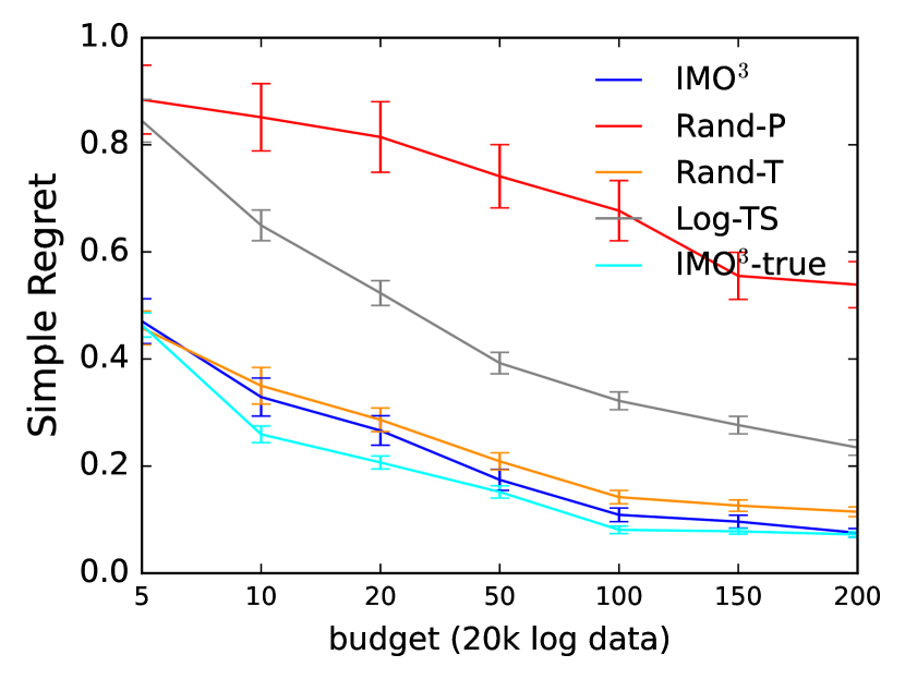
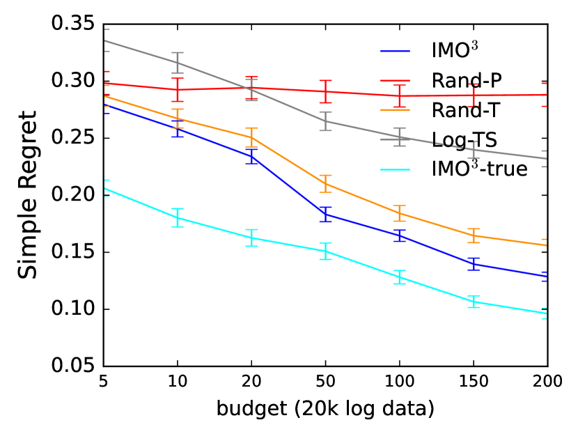
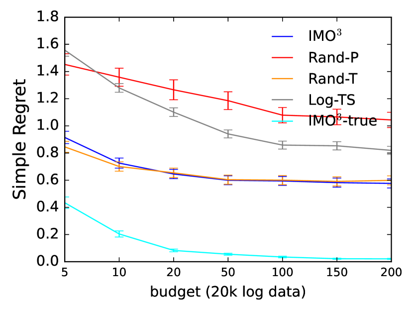
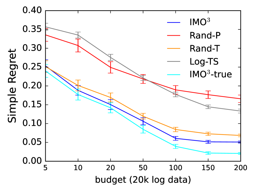
For each of the four problems, we first fix the size of the logged dataset and assess how simple regret ((lower the better)) varies with the interaction budget $T$. The results are shown in Figure 1. Each result is averaged over ten logged datasets generated for each problem, ten randomly sampled $\theta_{*}$, and 5 repeated runs under each combination of the logged data and $\theta_{*}$ (error bars represent standard error). We see that $\tt IMO^{3}$ outperforms or performs comparably to our baselines in all four problems. While Rand-T is similar to the pre-selection phase of $\tt IMO^{3}$ and performs relatively well, its exploration is less efficient and limited by the budget, and thus is worse than $\tt IMO^{3}$. This illustrates the advantage of using G-optimal design with a sufficient number of pre-selected policies to query the designer for feedback. The gap between $\tt IMO^{3}$ using estimated vs. true values is due to errors in value estimation—see the second term in our regret bound (Section 5.3). This term is invariant w.r.t. $T$, thus the gap remains relatively constant as $T$ varies in our experiments.

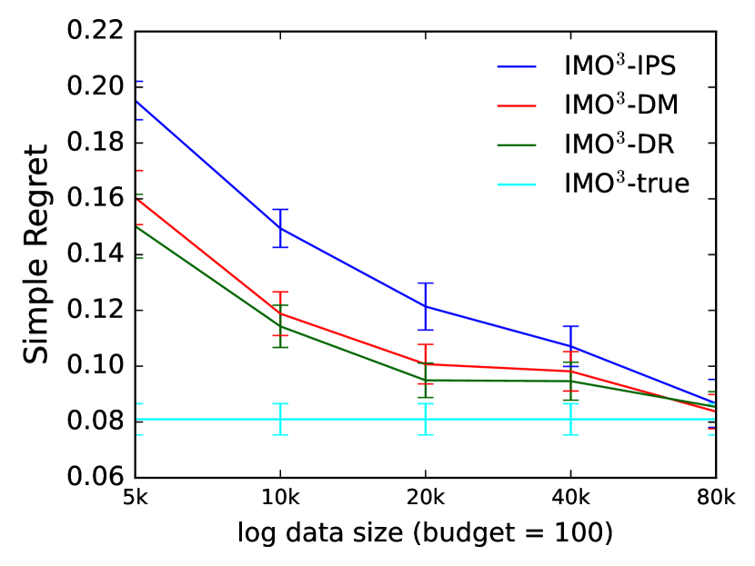
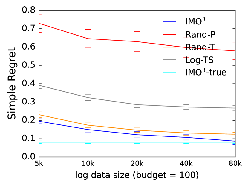
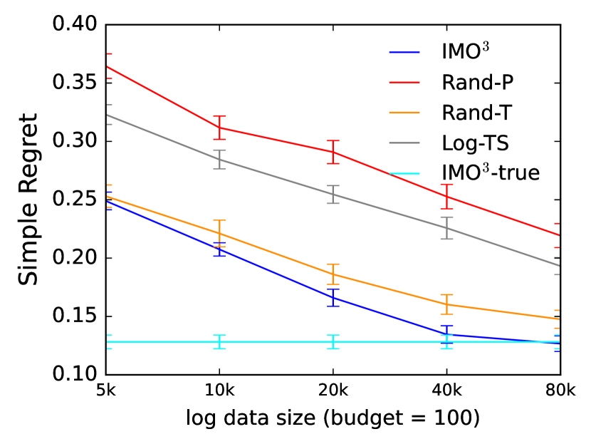
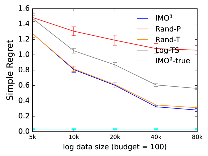
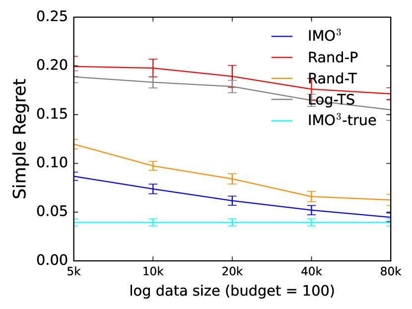
We further study how the amount of logged data influences the simple regret of $\tt IMO^{3}$. We fix $T=100$, and vary the size of the logged dataset used for policy-value estimation. Intuitively, if the dataset is sufficient to provide an accurate value estimate for any policy, $\tt IMO^{3}$ should perform similarly to directly using true values. Results in Figure 2 show that when the logged dataset is small, inaccurate value estimates cause algorithms that rely on off-policy estimates to perform poorly compared to using true values. As the size of the dataset increases, the decrease in value-estimation error allows $\tt IMO^{3}$ to outperform the baselines by selecting the most effective policies for querying the designer. When the logged dataset is sufficiently large, more accurate value estimates ensure that $\tt IMO^{3}$ converges to the that of using true values.

7 Related Work

Drugan and Nowé Drugan and Nowé (2013) is the first work to propose, analyze and experiment with a $\tt UCB1$ algorithm with a scalarized objective for MOO and a Pareto $\tt UCB1$ algorithm. Auer et al. Auer et al. (2016) formulate the problem of Pareto-frontier identification as a BAI problem. Thompson sampling in MOO is studied (though not theoretically analyzed) by Yahyaa and Manderick Yahyaa and Manderick (2015). Two recent works apply Gaussian process (GP) bandits to MOO. Paria et al. Paria et al. (2019) model the posterior of each objective function as a GP and minimize regret w.r.t. a known distribution of scalarization vectors. Zhang and Golovin Zhang and Golovin (2020) show that this algorithm generates a set of points that maximize random hypervolume scalarization, a objective often used in practice. All above works are in the online setting, where the learning agent interactively probes the environment to learn about its objective functions. Our setting is offline and the objective functions are estimated from logged data collected by some prior policy.

In terms of the motivation, the closest work to ours is that of Roijers et al. Roijers et al. (2017), who treat online MOO as a two-stage problem, where the objective functions are estimated using initial interactions with the environment and the scalarization vector is then estimated via user interaction. Unlike our work, they do not propose a specific algorithm for their setting, but only adapts existing bandit algorithms based on learned utility functions. Besides, they do not formulate the problem as off-policy optimization, and thus the process can be costly.

8 Conclusion

In this work, we study the problem of multi-objective optimization with unknown objective functions. We propose an interactive off-policy optimization algorithm for finding the optimal policy that achieves the desired trade-off among objectives. Specifically, we adapt off-policy estimators to evaluate policy values on all objectives, choose policies that effectively elicit a designer’s preference trade-offs, and learn the optimal policy using best arm identification. We prove upper bounds on the simple regret or our method and demonstrate it effectiveness with experiments on four MOO problems.

For future work, we plan to generalize (and analyze) our algorithm to more complex utility functions and other types of query models. We applied G-optimal design for BAI to provide theoretical guarantees—using other BAI algorithms for MOO is of interest.

Appendix A Off-Policy Optimization

Claim 1.

Using the DM estimator (3), problem (6) is maximization of a linear function with linear constraints.

The claim is proved as follows. By definition, $\hat{V}^{\textsc{dm}}(\pi)$ is linear in $\pi$, and so is $\theta^{\top}\hat{V}^{\textsc{dm}}(\pi)$ for any $\theta$. The set $\Pi$ is an intersection of halfspaces, as discussed below (1). ∎

Claim 2.

Using the IPS estimator (4), problem (6) is maximization of a linear function with linear constraints.

Under the assumption that the rewards are non-negative, any clipped policy $\pi$, where $\pi(a\mid x)/\pi_{0}(a\mid x)>M$ for all $x$ and $a$, can be replaced with an unclipped policy with at least as high value. Let

$$\Pi^{\prime}=\left\{\pi\in\Pi:\pi(a\mid x)\leq M\pi_{0}(a\mid x),\ \forall x\in\mathcal{X},a\in\mathcal{A}\right\}$$

be the set of all unclipped policies. This set has two key properties. First, it is an intersection of halfspaces, since $\Pi$ is and the additional constraints are linear in $\pi$. Second, for any $\pi\in\Pi^{\prime}$, the minimum in (4) can be omitted. In turn, $\hat{V}^{\textsc{ips}}(\pi)$ becomes linear in $\pi$ and so does $\theta^{\top}\hat{V}^{\textsc{ips}}(\pi)$ for any $\theta$. ∎

Claim 3.

Using the DR estimator (5), the problem (6) is maximization of a linear function with linear constraints.

The claim is proved as follows. By definition, $\hat{V}^{\textsc{dr}}(\pi)$ is linear in $\pi$, and so is $\theta^{\top}\hat{V}^{\textsc{dr}}(\pi)$ for any $\theta$. The set $\Pi$ is an intersection of halfspaces, as discussed below (1). ∎

Appendix B Regret Analysis

This section is organized as follows. Theorem 1 gives a general simple regret bound of a BAI algorithm for MOO, which decomposes into the simple regret of the algorithm based on estimated policy values, and a second term that accounts for errors in off-policy estimated values. In Theorem 2, we bound the simple regret of $\tt IMO^{3}$ based on off-policy estimated values. In Theorem 3, we bound the error induced by the IPS estimator.

Theorem 1.

For any policy $\pi\in\Pi$, let $||\hat{V}(\pi)-V(\pi)||_{2}\leq\varepsilon$ hold with probability at least $1-\delta$. Then the simple regret of $\tt IMO^{3}$ is

$$R_{T}^{sim}\leq\hat{R}_{T}^{sim}+2\varepsilon||\theta_{*}||_{2}$$

with probability at least $1-2\delta$, where $\hat{R}_{T}^{sim}=u_{\theta_{*}}(\hat{V}(\hat{\pi}_{*}))-u_{\theta_{*}}(\hat{V}(\tilde{\pi}_{*}))$ and $\hat{\pi}_{*}=\operatorname*{arg\,max\,}_{\pi\in\Pi}u_{\theta_{*}}\big{(}\hat{V}(\pi)\big{)}$ are the simple regret and optimal policy with respect to the estimated policy values, respectively.

Proof.

First recall that $\pi_{\ast}=\operatorname*{arg\,max\,}_{\pi\in\Pi}\theta_{\ast}^{\top}V(\pi)$ is the optimal policy with respect to true values, $\hat{\pi}_{\ast}=\operatorname*{arg\,max\,}_{\pi\in\Pi}\theta_{\ast}^{\top}\hat{V}(\pi)$ is the optimal policy with respect to estimated values, and $\tilde{\pi}_{\ast}$ is the output of the $\tt IMO^{3}$ algorithm. The simple regret is

$$R_{T}^{sim} =\theta_{\ast}^{\top}V(\pi_{*})-\theta_{\ast}^{\top}V(\tilde{\pi}_{*})$$

$$=\theta_{\ast}^{\top}V(\pi_{*})-\theta_{\ast}^{\top}\hat{V}(\hat{\pi}_{*})+\theta_{\ast}^{\top}\hat{V}(\hat{\pi}_{*})-\theta_{\ast}^{\top}V(\tilde{\pi}_{*})$$

$$\leq\theta_{\ast}^{\top}V(\pi_{*})-\theta_{\ast}^{\top}\hat{V}(\pi_{*})+\theta_{\ast}^{\top}\hat{V}(\pi_{*})-\theta_{\ast}^{\top}\hat{V}(\hat{\pi}_{*})+\theta_{\ast}^{\top}\hat{V}(\hat{\pi}_{*})-\theta_{\ast}^{\top}\hat{V}(\tilde{\pi}_{*})+\theta_{\ast}^{\top}\hat{V}(\tilde{\pi}_{*})-\theta_{\ast}^{\top}V(\tilde{\pi}_{*})\,.$$

Note that $\hat{R}_{T}^{sim}=\theta_{\ast}^{\top}\hat{V}(\hat{\pi}_{*})-\theta_{\ast}^{\top}\hat{V}(\tilde{\pi}_{*})$ and $\theta_{\ast}^{\top}\hat{V}(\pi_{*})-\theta_{\ast}^{\top}\hat{V}(\hat{\pi}_{*})\leq 0$. Therefore,

$$R_{T}^{sim} \leq\hat{R}_{T}^{sim}+\theta_{\ast}^{\top}V(\pi_{*})-\theta_{\ast}^{\top}\hat{V}(\pi_{*})+\theta_{\ast}^{\top}\hat{V}(\tilde{\pi}_{*})-\theta_{\ast}^{\top}V(\tilde{\pi}_{*})$$

$$\leq\hat{R}_{T}^{sim}+|\theta_{\ast}^{\top}V(\pi_{*})-\theta_{\ast}^{\top}\hat{V}(\pi_{*})|+|\theta_{\ast}^{\top}\hat{V}(\tilde{\pi}_{*})-\theta_{\ast}^{\top}V(\tilde{\pi}_{*})|$$

$$\leq\hat{R}_{T}^{sim}+||\theta_{\ast}||_{2}||V(\pi_{*})-\hat{V}(\pi_{*})||_{2}+||\theta_{\ast}||_{2}||\hat{V}(\tilde{\pi}_{*})-V(\tilde{\pi}_{*})||_{2}\,,$$

where the last step is by the Cauchy-Schwarz inequality. Finally, $||\hat{V}(\pi)-V(\pi)||_{2}\leq\varepsilon$ holds for any policy $\pi$ with probability at least $1-\delta$, and thus

$$R_{T}^{sim}\leq\hat{R}_{T}^{sim}+2\varepsilon||\theta_{\ast}||_{2}$$

holds with probability at least $1-2\delta$ by the union bound. This concludes the proof. ∎

The general bound in Theorem 1 decomposes into two parts. The first term $\hat{R}_{T}^{sim}$ is the regret of BAI based on estimated policy values and reflects the amount of the designer’s feedback. We bound it for $\tt IMO^{3}$ in Theorem 2. The second term accounts for errors in off-policy estimates. We bound the off-policy error $\varepsilon$ in Theorem 3. Both theorems are stated and proved below.

Theorem 2.

Let $c_{\min},\delta>0$ be chosen such that

$$\min_{v\in\mathcal{V}}\min\{h^{\prime}(v^{\top}\theta_{*}),h^{\prime}(v^{\top}\hat{\theta})\}\geq c_{\min}$$

holds with probability at least $1-\delta$. Then

$$\hat{R}_{T}^{sim}\leq L\exp\left[-\frac{\Delta_{\min}^{2}c_{\min}^{2}T}{2g(\alpha_{*})}\right]$$

holds with probability at least $1-\delta$.

Proof.

Let $\hat{\theta}$ be the MLE of model parameters returned by $\tt IMO^{3}$, estimated from a dataset of size $T$ collected according to the optimal design $\alpha_{*}$. Let $\hat{\mu}_{i}=v_{i}^{\top}\hat{\theta}$ be the corresponding utility estimate. To simplify exposition, we do not analyze the effect of rounding in the optimal design and assume that all $\alpha_{*}(i)$ are multiples of $1/T$. In this case, each $v_{i}$ appears in the collected dataset exactly $\alpha_{*}(i)T$ times. This is a standard assumption in the analyses with optimal designs.

Now we are ready to bound the simple regret of our solution. Let $I$ be the index of the policy chosen by our algorithm. Then

$$\hat{R}_{T}^{sim} =\mathbb{E}\left[\mu_{1}-\mu_{I}\right]\leq\mathbb{P}\left(I>1\right)\leq\sum_{i=2}^{L}\mathbb{P}\left(\hat{\mu}_{i}\geq\hat{\mu}_{1}\right)\leq\sum_{i=2}^{L}(\mathbb{P}\left(\hat{\mu}_{i}\geq\mu_{i}+\Delta_{i}/2\right)+\mathbb{P}\left(\hat{\mu}_{1}\leq\mu_{1}-\Delta_{i}/2\right))$$

$$=\sum_{i=2}^{L}(\mathbb{P}\left(\hat{\mu}_{i}-\mu_{i}\geq\Delta_{i}/2\right)+\mathbb{P}\left(\mu_{1}-\hat{\mu}_{1}\geq\Delta_{i}/2\right))\,.$$

The first inequality follows from $\mu_{i}\in[0,1]$ and the second is a result of applying a union bound over all policies. In the third inequality, we use that $a\geq b$ implies that either $a\geq c$ or $b\leq c$ holds for any $c$, which we choose as $c=(\mu_{i}+\mu_{1})/2$.

By Lemma 1 in Kveton et al. [2020], the MLE $\hat{\theta}$ in a GLM satisfies

$$\hat{\theta}-\theta_{*}=\Lambda^{-1}\sum_{t=1}^{T}X_{t}\varepsilon_{t}\,,$$

where $X_{t}=\hat{V}(\pi_{t})$ are estimated values in round $t$ and $\varepsilon_{t}$ is observation noise. Note that the noise is $\sigma^{2}$-sub-Gaussian for $\sigma=1/2$. Moreover, $\Lambda=\sum_{t=1}^{T}h^{\prime}(X_{t}^{\top}\tilde{\theta})X_{t}X_{t}^{\top}$ is the sample covariance matrix weighted by the derivative of $h$ at $\tilde{\theta}$, a convex combination of $\hat{\theta}$ and $\theta_{*}$. After this decomposition, we can apply Hoeffding’s inequality to a sum of weighted sub-Gaussian random variables and get

$$\mathbb{P}\left(\hat{\mu}_{i}-\mu_{i}\geq\Delta_{i}/2\right) =\mathbb{P}\left(v_{i}^{\top}(\hat{\theta}-\theta_{*})\geq\Delta_{i}/2\right)\leq\exp\left[-\frac{\Delta_{i}^{2}}{8\sigma^{2}v_{i}^{\top}\Lambda^{-1}G\Lambda^{-1}v_{i}}\right]=\exp\left[-\frac{\Delta_{i}^{2}}{2v_{i}^{\top}\Lambda^{-1}G\Lambda^{-1}v_{i}}\right]$$

for any $i\in[L]$, where $G=\sum_{t=1}^{T}X_{t}X_{t}^{\top}$.

Now we make three observations. First, since $\tilde{\theta}$ is a convex combination of $\hat{\theta}$ and $\theta_{*}$, and the derivative of the logistic function is monotone, we have $h^{\prime}(X_{t}^{\top}\tilde{\theta})\geq c_{\min}$. Second, since $h^{\prime}(X_{t}^{\top}\tilde{\theta})\geq c_{\min}$, we have $c_{\min}G\preceq\Lambda$ and thus $c_{\min}^{-1}G^{-1}\succeq\Lambda^{-1}$. Third, since our optimal design is applied exactly, $G=TG_{\alpha_{*}}$. It follows that

$$v_{i}^{\top}\Lambda^{-1}G\Lambda^{-1}v_{i}\leq c_{\min}^{-2}v_{i}^{\top}G^{-1}v_{i}=c_{\min}^{-2}T^{-1}v_{i}^{\top}G_{\alpha_{*}}^{-1}v_{i}\,,$$

and in turn

$$\mathbb{P}\left(\hat{\mu}_{i}-\mu_{i}\geq\Delta_{i}/2\right)\leq\exp\left[-\frac{\Delta_{i}^{2}c_{\min}^{2}T}{2v_{i}^{\top}G_{\alpha_{*}}^{-1}v_{i}}\right]\leq\exp\left[-\frac{\Delta_{i}^{2}c_{\min}^{2}T}{2g(\alpha_{*})}\right]\,.$$

Finally, we chain all inequalities and get

$$\hat{R}_{T}^{sim}\leq 2\sum_{i=1}^{L}\exp\left[-\frac{\Delta_{i}^{2}c_{\min}^{2}T}{2g(\alpha_{*})}\right]\leq L\max_{i\in[L]}\exp\left[-\frac{\Delta_{i}^{2}c_{\min}^{2}T}{2g(\alpha_{*})}\right]=L\exp\left[-\frac{\Delta_{\min}^{2}c_{\min}^{2}T}{2g(\alpha_{*})}\right]\,.$$

This concludes the proof. ∎

Theorem 3.

For any fixed policy $\pi$ and $\delta\in(0,1)$, the error in the value estimate by the IPS estimator is $||\hat{V}^{\textsc{IPS}}(\pi)-V(\pi)||_{2}\leq\sqrt{\frac{dM^{2}\log(2d/\delta)}{2N}}$ with probability at least $1-\delta$, where $d$ is the number of objectives, $M$ is the tunable parameter in the IPS estimator, and $N$ is the size of logged data.

Proof.

For any objective $i\in[d]$, we can apply Hoeffding’s inequality to the random variables $X_{j}=\min\Big{\{}M,\frac{\pi(a_{j}\mid x_{j})}{\pi_{0}(a_{j}\mid x_{j})}\Big{\}}r_{j}$ and get that $|\hat{V}_{i}^{\textsc{ips}}(\pi)-V_{i}(\pi)|\leq M\sqrt{\frac{\log(2d/\delta)}{2N}}$ holds with probability at least $1-\delta/d$ Strehl et al. [2010]. By the union bound,

$$||\hat{V}^{\textsc{IPS}}(\pi)-V(\pi)||_{2}=\sqrt{\sum_{i=1}^{d}(\hat{V}_{i}^{\textsc{ips}}(\pi)-V_{i}(\pi))^{2}}\leq\sqrt{\frac{dM^{2}\log(2d/\delta)}{2N}}$$

holds with probability at least $1-\delta$. This concludes the proof. ∎

Finally, we substitute the bounds from Theorems 2 and 3 to Theorem 1, which leads to Section 5.3.

Appendix C Experiments

C.1 Multi-Objective Optimization Problems

ZDT1.  The ZDT test suite Zitzler et al. [2000] is the most widely employed benchmark for MOO. We use ZDT1, the first problem in the test suite, a box-constrained $n$-dimensional two-objective problem, with objectives $F_{1}$ and $F_{2}$ defined as

$$F_{1}(x)=5x_{1},\quad F_{2}(x)=g(x)\bigg{[}1-\sqrt{\frac{x_{1}}{g(x)}}\bigg{]}\,,$$ (10)

$$\textrm{and }\;g(x)=1+\frac{9(\sum_{i=2}^{n}x_{i})}{n-1}\,,$$

where $x=(x_{i})_{i=1}^{n}$ and $x_{i}\in[0,1],\forall i\in[n]$. We use $n=5$ in our experiments, treating $(x_{4},x_{5})$ as context, and perform optimization on $(x_{i})_{i=1}^{3}$. We sample five combinations of $(x_{4},x_{5})$ uniformly to create $\mathcal{X}$ and ten combinations of $(x_{i})_{i=1}^{3}$ to create the action set $\mathcal{A}$. For each context $x\in\mathcal{X}$, the logging policy is a distribution sampled from a Dirichlet $\pi_{0}(\cdot\mid x)\sim\mathrm{Dir}(\alpha)$ ($\alpha$ is a $10$-D vector, $\alpha_{i}=10,\forall i\in[10]$). To generate a logged record in $\mathcal{D}$, we randomly select a context $x$, use $\pi_{0}(\cdot\mid x)$ to select an action, and generate its 2-D reward using $F_{1}$ and $F_{2}$ with added zero-mean Gaussian noise $N(0,0.5^{2})$.
Crashworthiness.  This MOO problem is extracted from a real-world crashworthiness domain de Carvalho et al. [2018], where three objectives factor into the optimization of the crash-safety level of a vehicle. We refer to Sec. 2.1 of de Carvalho et al. [2018] for detailed objective functions and constraints. We omit the constants in their objective functions to ensure the three objectives lie in a similar range (if one objective dominates the others, the problem may reduce to a single objective problem). Five bounded decision variables $(x_{i})_{i=1}^{5}$ represent the thickness of reinforced members around the car front. We use the last two variables as contexts and the first three as actions. The rest settings of the simulation are the same as for ZDT1.
Stock Investment.  The stock investment problem is a widely studied real-world MOO problem Liang and Qu [2013], where we need to trade off returns and volatility of an investment strategy. We consider investing one dollar in a stock at the end of each day as an action and try to optimize the relative gain and volatility of this investment at the end of the next day. Specifically, the relative gain is the stock’s closing price on the second day minus that on the first day, and we use the absolute difference as a measure of investment volatility. Our goal is to maximize the relative gain and minimize the volatility between two consecutive days of a one-dollar investment, on average.

We use 48 popular stocks, including CSCO, UAL, BA, BBY, BAC, LYFT, PEP, COST, LOW, SBUX, AMZN, INTC, GM, ATT, KO, MSFT, UBER, AMD, PINS, NVDA, BBBY, FDX, AXP, FB, IBM, WFC, GS, DELL, NFLX, JPM, COF, MRNA, TSLA, BYND, AAL, JD, GOOG, PFE, FORD, MS, ZM, DAL, BABA, MA, TGT, AAPL, WMT, CRM as the action set $\mathcal{A}$. We use the four quarters of a year as the context set $\mathcal{X}$. To create logged data, we first collect the closing stock prices from Yahoo Finance for the period Nov.1/2020–Nov.1/2021. For each context $x\in\mathcal{X}$, the logging policy is a distribution sampled from a Dirichlet $\pi_{0}(\cdot\mid x)\sim\mathrm{Dir}(\alpha)$ ($\alpha$ is a $48$-D vector with $\alpha_{i}=10,\forall i\in[48]$). To generate each logged record, we uniformly sample a context/quarter $x$, sample an action/stock for investment from $\pi_{0}(\cdot\mid x)$, and sample the two-D reward vector by randomly choosing two consecutive days in the quarter and the selected stock’s closing prices on these days to compute relative gain and volatility. We estimate the value $\hat{V}(\pi)$ of policy $\pi$ using this logged data and compute its true expected value $V(\pi)$ using the original data.
Yahoo! News Recommendation.  This is a news article recommendation problem derived from the Yahoo! Today Module click log dataset (R6A). We consider two objectives to maximize, the click through rate (CTR) and diversity of the recommended articles. In the original dataset, each record contains the recommended article, the click event (0 or 1), the pool of candidate articles, and a 6-dimensional feature vector for each article in the pool. The logged recommendation is selected from the pool uniformly. We adopt the original click event in the logged dataset to measure CTR of the recommendation, and use the $\ell_{2}$ distance between the recommended article’s feature and the average feature vector in the pool to represent the diversity of this recommendation.

For our experiments, we extract five different article pools as contexts and all logged records associated with them from the original data, resulting in 1,123,158 records in total. Each article pool has 20 candidates as actions. To generate a recommendation record in the logged data of certain size, we first randomly sample an article pool as the context, and then sample a record from the original data associated with this article pool. Note that in this way we inherit the uniform logging policy of the original data. To aid visualization, we multiply CTR and diversity by 10, so estimated values are not too small. We add zero-mean Gaussian noise ($N(0,0.5^{2})$) to the diversity of each logged recommendation to introduce observational noise. The true policy value is estimated using the full, original dataset without added noise.

C.2 Regret Analysis of Log-TS for BAI

[]lemmaregretaverage For any $\delta\in(0,1)$ and the average policy $\tilde{\pi}_{*}=\sum_{t=1}^{T}\pi_{t}/T$ from Log-TS, the simple regret is $\hat{R}_{T}^{sim}=\tilde{O}(d^{\frac{3}{2}}\sqrt{\log(1/\delta)/T})$ with probability at least $1-\delta$.

Proof.

Let $\mu(x)=1/(1+\exp[-x])$ be the sigmoid function. Let $v_{*}=\hat{V}(\hat{\pi}_{*})$ be the optimal arm under estimated policy values and $V_{t}=\hat{V}(\pi_{t})$ be the arm pulled by $\tt IMO^{3}$ in round $t\in[T]$. Then, from Abeille and Lazaric [2017], the expected $n$-round regret of TS in a logistic bandit, which is $\tt IMO^{3}$ in this case, is

$$T\mu(\theta_{*}^{\top}v_{*})-\sum_{t=1}^{T}\mu(\theta_{*}^{\top}V_{t})=\tilde{O}(d^{\frac{3}{2}}\sqrt{T\log(1/\delta)})$$

with probability at least $1-\delta$, for any $\delta\in(0,1)$. Now note that $x-y\leq\alpha^{-1}(\mu(x)-\mu(y))$ holds for any $x>y$, where $\alpha=\min\left\{\dot{\mu}(x),\dot{\mu}(y)\right\}$ is the minimum derivative of $\mu$ at $x$ and $y$. Since $\|\theta_{*}\|_{2}$, $\|v_{*}\|_{2}$, and $\|v_{t}\|_{2}$ are bounded, $\alpha$ is bounded away from zero and thus $\alpha^{-1}$ is bounded away from infinity. Thus $\alpha$ can be treated as a constant and

$$T\theta_{*}^{\top}v_{*}-\sum_{t=1}^{T}\theta_{*}^{\top}V_{t}=\tilde{O}(d^{\frac{3}{2}}\sqrt{T\log(1/\delta)})\,.$$

Finally we note that

$$\hat{R}_{T}^{sim}=\frac{1}{T}T\theta_{*}^{\top}v_{*}-\frac{1}{T}\sum_{t=1}^{T}\theta_{*}^{\top}V_{t}=\tilde{O}(d^{\frac{3}{2}}\sqrt{\log(1/\delta)/T})\,.$$

∎

C.3 $\tt IMO^{3}$ with Different Off-Policy Estimators

Besides the IPS estimator, we also apply DM and DR estimators in $\tt IMO^{3}$, to show how $\tt IMO^{3}$ performs with different off-policy estimators. We only evaluate DM and DR estimators on the first three problems. As the logging policy used to collect the original Yahoo! Today Module click data is already a uniform policy, DM and DR estimators are exactly the same as the IPS estimator. For each of the first three problems in Section 6, we first build a reward model learned from the logged data, and then apply the model in DM and DR estimators. Specifically, for the DM estimator, we simply use the empirical mean of an action as its estimated value.

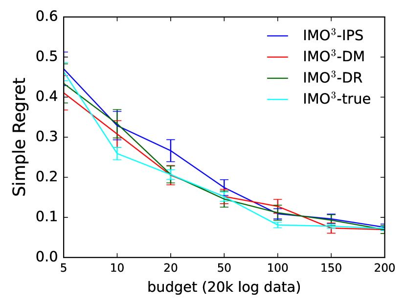
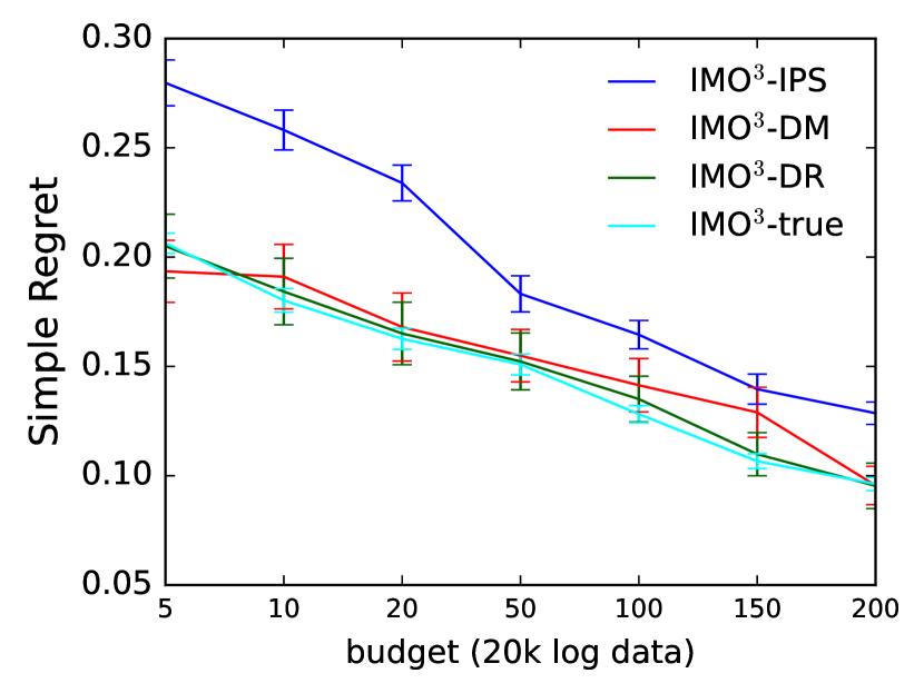
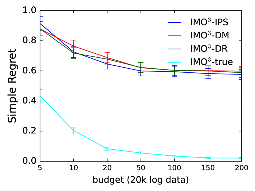
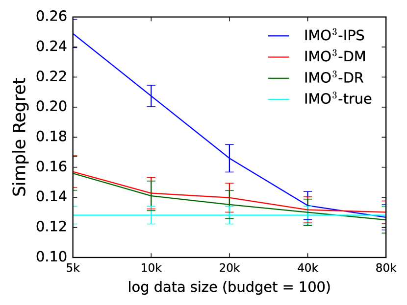
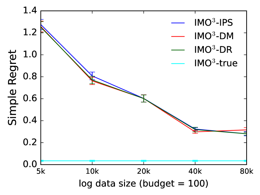
We follow the experimental setting in Section 6.3, and show the performance of the three estimators in Figures 3 and 4. We observe that $\tt IMO^{3}$ performs consistently well with all three estimators, which demonstrates the robustness of our method. Besides, the DM and DR estimators can achieve comparable or even better performance than the IPS estimator across different problems, which may be due to the higher variance of IPS. In particular, when the logging policy used to generate logged data has small probabilities on certain actions, it can lead to high variance in the value estimates. The DR estimator is usually slightly better than the other two, which demonstrates the improved performance with a better off-policy estimator.

(a) ZDT1.

(b) Crashworthiness.

(c) Stock investment.

Figure 3: Simple regret of different algorithms by fixing logged data size $N=20,000$ and varying budget. Each experiment is averaged over 10 logged data, 10 randomly selected $\theta_{*}$ and 5 runs under each combination of logged data and $\theta_{*}$.

(a) ZDT1.

(b) Crashworthiness.

(c) Stock investment.

Figure 4: Simple regret of different algorithms by fixing budget $T=100$ and varying logged data size. Each experiment is averaged over 10 logged data, 10 randomly selected $\theta_{*}$ and 5 runs under each combination of logged data and $\theta_{*}$.

References

- Abeille and Lazaric [2017] Marc Abeille and Alessandro Lazaric. Linear thompson sampling revisited. In AISTATS, 2017.
- Auer et al. [2016] Peter Auer, Chao-Kai Chiang, Ronald Ortner, and Madalina M. Drugan. Pareto front identification from stochastic bandit feedback. In AISTATS, 2016.
- Beygelzimer and Langford [2009] Alina Beygelzimer and John Langford. The offset tree for learning with partial labels. KDD, 2009.
- Boutilier [2002] Craig Boutilier. A POMDP formulation of preference elicitation problems. 2002.
- Boutilier [2013] Craig Boutilier. Computational decision support: Regret-based models for optimization and preference elicitation. In Comparative Decision Making: Analysis and Support Across Disciplines and Applications. 2013.
- Branke et al. [2008] J. Branke, K. Deb, Kaisa Miettinen, and R. Slowinski. Multiobjective Optimization: Interactive and Evolutionary Approaches. Springer-Verlag, 2008.
- Camerer [2004] Colin F. Camerer. Advances in Behavioral Economics. 2004.
- de Carvalho et al. [2018] Vinicius Renan de Carvalho, Jaime Simão, and Sichman. Solving real-world multi-objective engineering optimization problems with an election-based hyper-heuristic. 2018.
- Deaton and Cartwright [2018] Angus Deaton and Nancy Cartwright. Understanding and misunderstanding randomized controlled trials. Social Science & Medicine, 2018.
- Drugan and Nowé [2013] Madalina M. Drugan and Ann Nowé. Designing multi-objective multi-armed bandits algorithms: A study. In Proceedings of the 2013 International Joint Conference on Neural Networks, 2013.
- Dudik et al. [2011] Miroslav Dudik, John Langford, and Lihong Li. Doubly robust policy evaluation and learning. ICML, 2011.
- Dudík et al. [2015] Miroslav Dudík, Katja Hofmann, Robert E. Schapire, Aleksandrs Slivkins, and Masrour Zoghi. Contextual dueling bandits. In COLT, 2015.
- Jamieson and Talwalkar [2016] Kevin Jamieson and Ameet Talwalkar. Non-stochastic best arm identification and hyperparameter optimization. In AISTATS. PMLR, 2016.
- Karnin et al. [2013] Zohar Karnin, Tomer Koren, and Oren Somekh. Almost optimal exploration in multi-armed bandits. In ICML, 2013.
- Keeney and Raiffa [1976] Ralph L. Keeney and Howard Raiffa. Decisions with Multiple Objectives: Preferences and Value Trade-offs. Wiley, 1976.
- Kohavi and Longbotham [2011] Ron Kohavi and Roger Longbotham. Unexpected results in online controlled experiments. SIGKDD Explor. Newsl., 2011.
- Kohavi et al. [2009] Ron Kohavi, Roger Longbotham, Dan Sommerfield, and Randal M. Henne. Controlled experiments on the web: Survey and practical guide. KDD, 2009.
- Kveton et al. [2020] Branislav Kveton, Manzil Zaheer, Csaba Szepesvari, Lihong Li, Mohammad Ghavamzadeh, and Craig Boutilier. Randomized exploration in generalized linear bandits. In AISTATS, 2020.
- Lambert and Pregibon [2007] Diane Lambert and Daryl Pregibon. More bang for their bucks: assessing new features for online advertisers. SIGKDD Explor., 2007.
- Lattimore and Szepesvári [2020] Tor Lattimore and Csaba Szepesvári. Bandit Algorithms. Cambridge University Press, 2020.
- Liang and Qu [2013] J. J. Liang and B. Y. Qu. Large-scale portfolio optimization using multiobjective dynamic mutli-swarm particle swarm optimizer. In 2013 IEEE Symposium on Swarm Intelligence, 2013.
- Mas-Colell et al. [1995] Andreu Mas-Colell, Micheal D. Whinston, and Jerry R. Green. Microeconomic Theory. Oxford University Press, 1995.
- McFadden [1974] Daniel McFadden. Conditional logit analysis of qualitative choice behavior. In Frontiers in Econometrics. 1974.
- Paria et al. [2019] Biswajit Paria, Kirthevasan Kandasamy, and Barnabás Póczos. A flexible framework for multi-objective bayesian optimization using random scalarizations. In UAI, 2019.
- Roijers et al. [2017] Diederik M. Roijers, Luisa M. Zintgraf, and Ann Nowé. Interactive thompson sampling for multi-objective multi-armed bandits. In ADT, 2017.
- Rosenbaum and Rubin [1983] Paul R. Rosenbaum and Donald B. Rubin. The central role of the propensity score in observational studies for causal effects. Biometrika, 1983.
- Strehl et al. [2010] Alex Strehl, John Langford, Lihong Li, and Sham M Kakade. Learning from logged implicit exploration data. In NeurIPS, 2010.
- Swaminathan and Joachims [2015] Adith Swaminathan and Thorsten Joachims. Counterfactual risk minimization: Learning from logged bandit feedback. ICML, 2015.
- Tversky and Kahneman [1974] Amos Tversky and Daniel Kahneman. Judgment under uncertainty: Heuristics and biases. Science, 1974.
- Viappiani and Boutilier [2010] Paolo Viappiani and Craig Boutilier. Optimal Bayesian recommendation sets and myopically optimal choice query sets. In NeurIPS, 2010.
- Wong [1994] Weng Kee Wong. Comparing robust properties of a, d, e and g-optimal designs. Computational Statistics and Data Analysis, 1994.
- Yahyaa and Manderick [2015] Saba Q. Yahyaa and Bernard Manderick. Thompson sampling for multi-objective multi-armed bandits problem. In ESANN, 2015.
- Zhang and Golovin [2020] Richard Zhang and Daniel Golovin. Random hypervolume scalarizations for provable multi-objective black box optimization. In ICML, 2020.
- Zitzler et al. [2000] Eckart Zitzler, Kalyanmoy Deb, and Lothar Thiele. Comparison of multiobjective evolutionary algorithms: Empirical results. Evol. Comput., 2000.