Time distance based computation of the state space of preemptive real time systems.

Abstract

We explore in this paper a novel approach that builds an overapproximation of the state space of preemptive real time systems. Our graph construction extends the expression of a class to the time distance system that encodes the quantitative properties of past fired subsequences. This makes it possible to restore relevant time information that is used to tighten still more the DBM overapproximation of reachable classes. We succeed thereby to build efficiently tighter approximated graphs which are more appropriate to restore the quantitative properties of the model. The simulation results show that the computed graphs are of the same size as the exact graphs while improving by far the times needed for their computation.

url]http://www.lsi-usthb.dz/index.php?page=page32

1 Introduction   

Nowadays, real-time systems are becoming more and more complex and are often critical. Generally, these systems consist of several tasks that are timely dependent, interacting and sharing one or more resources (e.g processors, memory). Consequently, the correctness proofs of such systems are demanding much theory regarding their increasing complexity. We need, for instance, to consider formal models requiring the specification of time preemption; concept where execution of a task may be stopped for a while and later resumed at the same point. This notion of suspension implies to extend the semantics of timed clocks in order to handle such behaviors. For this effect, the concept of stopwatch has been introduced while many models have been defined, as for instance, hybrid automata ($LHA$) [1], stopwatch automata ($SWA$) [2], Network of Stopwatch Automta (NSA) [3], and timed automata with priorities [4]. Time Petri nets ($TPN$) have also been considered in several works including Preemptive-$TPN$ [5] [6] [7], Stopwatch- $TPN$ [8], Inhibitor-$TPN$ [9], Scheduling-$TPN$ [10] and of unfolding safe parametric stopwatch TPN (PSwPNs)[11]. For example, in [9] the authors defined the ITPN (Inhibitor arc Time Petri Nets) model, wherein the progression and the suspension of time is driven by using standard and inhibitor arcs.

However, whatever the model we consider, the time analysis of the system is basically the same, as it involves the investigation of a part of or the whole set of its reachable states that determines its state space. As the state space is generally infinite due to dense time semantics, we need therefore to compute finite abstractions of it, that preserve properties of interest. In these abstractions, states are grouped together, in order to obtain a finite number of these groups. These groups of states are, for instance, regions and zones for timed automata, or state classes [12] for time Petri nets. Hence, the states pertaining to each group can be described by a system of linear inequalities, noted $D$, whose set of solutions determines the state space of the group. Hence, if the model does not use any stopwatch, then $D$ is of a particular form, called DBM (Difference Bound Matrix) [13]. However, when using stopwatches, the system $D$ becomes more complex and does not fit anymore into a DBM.  In actual fact, $D$ takes a general polyhedral form whose canonical form [21] is given as a conjunction of two subsystems $D=\overrightarrow{D}\wedge\widehat{D},$ where $\overrightarrow{D}$ is a DBM system and $\widehat{D}$ is a polyhedral system that cannot be encoded with DBMs.

The major shortcoming of manipulating polyhedra is the performance loss in terms of computation speed and memory usage. Indeed, the complexity of solving a general polyhedral system is exponential in the worst case, while it is polynomial for a DBM system. Furthermore, the reachability is proved to be undecidable for both $\mathit{SWA}$ and $\mathit{LHA}$ [2] [1] [14], as well as for $TPN$ extended with stopwatches [8] [15]. As a consequence, the finiteness of the exact state class graph construction cannot be guaranteed even when the net is bounded.

In order to speed up the graph computation, an idea is to leave out the subsystem $\widehat{D},$ to keep only the system $\overrightarrow{D}$ thus overapproximating the space of $D$ to the DBM containing it, see [5][9][16] for details. The obvious consequence of the overapproximation is that we add states in the computed group that are not reachable indeed. Yet more, this could prevent the graph computation to terminate, by making the number of computed markings unbounded. Conversely, this can also make the computation of the approximated graph terminate by cutting off the polyhedral inequalities that prevent the convergence.

Furthermore, in order to settle a compromise between both techniques, a hybrid approach has been proposed by Roux et al [17]. The latter puts forward a sufficient condition that determines the cases where the subsystem $\widehat{D}$ becomes redundant in $D$. Hence, the combination of both DBM and polyhedral representations makes it possible to build the exact state class graph faster and with lower expenses in terms of memory usage comparatively to the polyhedra based approach [10]. More recently, Berthomieu et al have proposed an overapproximation method based on a quantization of the polyhedral system $D$ [8]. The latter approach ends in the exact computation of the graph in almost all cases faster than the hybrid approach [17]. Nevertheless, this technique is more costly in terms of computation time and memory usage comparatively to the DBM overapproximation although it yields much precise graphs.

Different algorithms [16][9][5] have been defined in the literature to compute the DBM overapproximation of a class. All these approaches are assumed theoretically to compute the tightest DBM approximation of $D$. However, we have shown in [16] that by avoiding to compute the minimal form of the DBM systems, our algorithm succeeds to compute straightforwardly the reachable systems in their normal form. We thereby shunned the computation and the manipulation of the intermediary polyhedra. Moreover, the effort needed for the normalization and the minimization of the resulted DBM system is removed. This has improved greatly the implementation and the computation of the DBM overapproximated graph.

Although the cost of computing the DBM overapproximation is low comparing to the exact construction, it remains that in certain cases the approximation is too coarse to restore properties of interest and especially quantitative properties [18]. In actual fact, more the approximated graphs are big more the approximation looses its precision and therefore includes false behaviors that may skew the time analysis of the system. Many of these false behaviors are generated in the DBM overapproximation because the computation of a DBM class is performed recursively only from its direct predecessor class. We think that some time information that stand in upper classes in the firing sequence could be used to fix the approximation of the class to compute. In actual fact, the DBM overapproximations defined in [16][9][5] are assumed to be the tightest when referring to the polyhhedral system $D$ computed in the context of the approximated graph. The latter may not be equal to the polyhedral system resulted after firing the same sequence in the exact graph. As polyhedral constraints are removed systematically each time they appear in upper classes in the firing sequence, the resulted $DBM$ overapproximation looses its precision. Therefore, the DBM overapproximation could be still more tightened if we could restore some time information encoded by polyhedral constraints removed in the upper classes in the firing sequence.

We explore in this paper a novel approach to compute a more precise DBM overapproximation of the state space of real time preemptive systems modeled by using the $\mathit{ITPN}$ model. For this effect, we extend the expression of a class to the time distance system that encodes the quantitative properties of firing’s subsequences. The time distance system has been already considered in the computation of the state space of many timed Petri nets extensions as [19] [20]. This system records relevant time information that is exploited to tighten still more the DBM overapproximation of a class. Although, the cost of computing the latter is slightly higher than when using classical DBM overapproximation techniques [16][9][5], the global effort needed to compute the final DBM system remains polynomial. Consequently, the resulted approximated graphs are very compact, even equal to the exact ones while improving by far their calculation times. Moreover, the obtained graphs are more suitable to restore quantitative properties of the model than other constructions. To advocate the benefits of this graph approximation, we report some experimental results comparing our graph constructions with other fellow approaches.

The remainder of this paper is organized as follows: In section 2, we present the syntax and the formal semantics of the $ITPN$ model. In section 3, we lay down and discuss through an example the algorithms that build the exact graph and the DBM overapproximation of an $ITPN$. In section 4, we introduce formally our overapproximation and show how the approximated graph is built. In $Section\ 5,$ we report the experimentation results of the implementation of our algorithms and compare them with those of other graph constructions.

2 Time Petri Net with Inhibitor Arcs

Time Petri nets with inhibitor arcs ($ITPN$) [9] extends time Petri nets[23] to Stopwatch inhibitor arcs. Formally, an $ITPN$ is defined as follows:

Definition 1

An $\mathit{ITPN}$ is given by the tuple $(P,T,B,F,M^{0},I,IH)$ where: $P$ and $T$ are respectively two nonempty sets of places and transitions; $B$ is the backward incidence function : $B:P\times T\longrightarrow\mathbb{N}=\{0,1,2,..\};$ $F$ is the forward incidence function $F:P\times T\longrightarrow\mathbb{N}$ ; $M^{0}$ is the initial marking mapping $M^{0}:P\longrightarrow\mathbb{N}$ ; $I$ is the delay mapping $I:T\longrightarrow\mathbb{Q}^{+}\times\mathbb{Q}^{+}\cup\left\{\infty\right\},$ where $\mathbb{Q}^{+}$ is the set of non negative rational numbers. We write $I(t)=[tmin(t),tmax(t)]$ such that $0\leq tmin(t)\leq tmax(t)$ ; $IH:P\times T\longrightarrow\mathbb{N}$  is the inhibitor arc function; there is an inhibitor arc connecting the place $p$ to the transition $t,$ if $IH(p,t)\neq 0.$

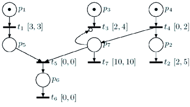
Figure 1: An $ITPN$ model

For instance, let us consider the $ITPN$ model shown in Fig 1. Therein, the inhibitor arc is the arc ended by a circle that connects the place $p_{7}$ to the transition $t_{3}$. Initially, the place $p_{3}$ is marked but the place $p_{7}$ is not; hence $t_{3}$ is enabled but not inhibited. Therefore, $t_{3}$ is progressing as it is the case for $t_{4}$ which is also enabled for the initial marking. However, the firing of the transition $t_{4}$ consumes the token in the place $p_{4}$ and produces another in $p_{2}$ and another one in $p_{7}$. Therefore, the inhibitor arc becomes activated and the clock of $t_{3}$ is thus suspended ($t_{3}$ is inhibited). This suspension lasts as long as $p_{7}$ remains marked. For more details, the formal semantics of the $ITPN$ model is introduced hereafter.

Let $RT:=(P,T,B,F,M^{0},I,IH)$ be an ITPN.

-

We call a marking the mapping, noted $M,$ which associates with each place a number of tokens: $M:P\rightarrow\mathbb{N}.$

-

A transition $t$ is said to be enabled for the marking $M,$ if $\forall p\in P,B(p,t)\leq M(p)$; the number of tokens in each input place of $t$ is greater or equal to the valuation of the arc connecting this place to the transition $t$. Thereafter, we denote by $Te(M)$ the set of transitions enabled for the marking $M$.

-

A transition $t$ is said to be inhibited for a marking $M,$ if it is enabled and if there exists an inhibitor arc connected to $t,$ such that the marking satisfies its valuation ($t\in Te(M))\wedge\exists p\in P,0<IH(p,t)\leq M(p)$. We denote by $Ti(M)$ the set of transitions that are inhibited for the marking $M$.

-

A transition $t$ is said to be activated for a marking $M,$ if it is enabled and not inhibited, ($t\in Te(M))\wedge$ $\ (t\notin Ti(M))$; we denote by $Ta(M)$ the set of transitions that are activated for the marking $M$.

-

Let $M$ be a marking ; two transitions $t_{i}$ and $t_{j}$ enabled for $M$ are said to be conflicting for $M$, if $\exists p\in P,\quad B(p,t_{i})+B(p,t_{j})>M(p).$

-

We note hereafter by $Conf(M)$ the relation built on $Te(M)^{2}$ such that $(t_{1},t_{2})\in Conf(M),$ iff $t_{1}$ and $t_{2}$ are in conflict for the marking $M$.

For instance, let us consider again the $ITPN$ of Fig 1. Its initial marking is equal to $M^{0}:\left\{p_{1},p_{3},p_{4}\right\}\rightarrow 1;\left\{p_{2},p_{5},p_{6},p_{7}\right\}\rightarrow 0.$ the sets of enabled, inhibited, and activated transitions for $M^{0}$ are respectively $Te(M^{0})=\left\{t_{1},t_{3,}t_{4}\right\},$ $Ti(M^{0})=\varnothing,$ and $Ta(M^{0})=Te(M^{0}).\vskip 6.0pt plus 2.0pt minus 2.0pt$

Remark 1

We assume in the sequel a monoserver semantics, which means that no transition can be enabled more than once for any marking.

We define the semantics of an $ITPN$ as follows:

Definition 2

The semantics of an $ITPN$ is defined as a LTS (labeled transition system), $ST=(\Gamma,e^{0},\rightarrow),$ such that:

• $\Gamma$ is the set of reachable states: Each state, noted $e,$ pertaining to $\Gamma$ is a pair $(M,V)$ where $M$ is a marking and $V$ is a valuation function that associates with each enabled transition $t$ of $Te(M)$ a time interval that gives the range of relative times within which $t$ can be fired. Formally we have : $\forall t$ $\in Te(M),\quad V(t):=[x(t),y(t)]$

• $e^{0}=(M^{0},V^{0})$ is the initial state, such that: $\forall t\in Te(M^{0}),\quad V^{0}(t):=I(t):=[tmin(t),tmax(t)].$

• $\rightarrow\in\Gamma\times(T\times\mathbb{Q}^{+})\times\Gamma$  is a relation, such that $((M,V),(t_{f},\underline{t_{f}}),(M^{\uparrow},V^{\uparrow}))\in\rightarrow,$ iff:

  (i)

  $t_{f}\in Ta(M).$

  (ii)

  $x(t_{f})\leq\underline{t_{f}}\leq\underset{\forall t\in Ta(M)}{MIN}\left\{y(t)\right\}.$

  and we have:

  $\forall p\in P,$ $M^{\uparrow}(p):=M(p)-B(p,t_{f})+F(p,t_{f})\vskip 3.0pt plus 1.0pt minus 1.0pt.$

  $\forall t\in Te(M^{\uparrow})$

  if $t$ $\notin New(M^{\uparrow})$:

      $[x^{\uparrow}(t),\ y^{\uparrow}(t)]:=[MAX(0,\ x(t)-\underline{t_{f}}),$ $\ y(t)-\underline{t_{f}}]$ $t\in Ta(M)$ $[x^{\uparrow}(t),\ y^{\uparrow}(t)]:=[x(t),$ $\ y(t)]$ $t\in Ti(M)$

  if $t$ $\in New(M^{\uparrow})$ 

  $\quad[x^{\uparrow}(t),\ y^{\uparrow}(t)]:=I(t)=[tmin(t),\ tmax(t)]$

  • where $New(M^{\uparrow})$ denotes the set of transitions newly enabled for the marking $M^{\uparrow}.$ These transitions are those enabled for $M^{\uparrow}$ and not for $M$, or those enabled for $M^{\uparrow}$ and $M$ but are conflicting with $t_{f}$  for the marking $M$.  Otherwise, an enabled transition which does not belong to $New(M^{\uparrow})$ is said to be persistent.

If $t$ is a transition enabled for the state $e$, we note $t$ the clock associated with $t$ that takes its values in $\mathbb{Q}^{+}.$ $t$ measures the residual time of the transition $t$ relatively to the instant where the state $e$ is reached. The time progresses only for activated transitions, whereas it is suspended for inhibited transitions. Therefore, a transition $t_{f}$ can be fired at relative time $\underline{t_{f}}$ from a reachable state $e,$ if $(i)$ $t_{f}$ is activated for the marking $M$, and if $(ii)$ the time can progress within the firing interval of $t_{f}$ without overtaking those of other activated transitions. After firing $t_{f}$ the reachable state, noted $e^{\uparrow},$ is obtained:

• by consuming a number of tokens in each input place $p$ of $t_{f}$ (given by the value $B(p,t_{f})$), and by producing a number of tokens in each output place $p$ of $t_{f}$ (given by the value $F(p,t_{f})$);

• by shifting the interval of a persistent activated transition with the value of the firing time of $t_{f}$. However, the intervals of persistent inhibited transitions remain unchanged. Finally, a newly enabled transition is assigned its static firing interval.

Similarly as for a $TPN,$ the behavior of an $ITPN$ can be defined as a sequence of pairs $(t_{f}^{i},\underline{t_{f}^{i}})$, where $t_{f}^{i}$ is a transition of the net and $\underline{t_{f}^{i}}$ $\in\mathbb{Q}^{+}$. Therefore, the sequence $\mathit{S}^{\mathit{\ast}}=((t_{f}^{1},\underline{t_{f}^{1}}),(t_{f}^{2},\underline{t_{f}^{2}}),..,(t_{f}^{n},\underline{t_{f}^{n}}))$ denotes that $t_{f}^{1}$ is firable after $\underline{t_{f}^{1}}$ time units, then $t_{f}^{2}$ is fired after $\underline{t_{f}^{2}}$ time units and so on, such that $t_{f}^{n}$ is fired after the absolute time $\sum_{i=1}^{n}\underline{t_{f}^{i}}.$ Moreover, we often express the behavior of the net as an untimed sequence, denoted by $\mathit{S}$, obtained from a timed sequence $\mathit{S}^{\mathit{\ast}}$ by removing the firing times: If $\mathit{S}^{\mathit{\ast}}=((t_{f}^{1},\underline{t_{f}^{1}}),(t_{f}^{2},\underline{t_{f}^{2}}),..,(t_{f}^{n},\underline{t_{f}^{n}})),$ then $\mathit{S}=(t_{f}^{1},t_{f}^{2},..,t_{f}^{n}).$ As the set of time values is assumed to be dense, the model $ST$ is infinite. In order to analyze this model, we need to compute an abstraction of it that saves the most properties of interest. The construction of a symbolic graph preserves the untimed sequences of $ST,$ and makes it possible to compute a finite graph in almost all cases. We show hereafter how to compute the state class graph of the $ITPN$ that preserves chiefly the linear properties of the model.

3 $ITPN$ state space construction

As for a $TPN$ model [23], the state graph $ST$ of an $ITPN$ can be contracted by gathering in a same class all the states reachable after firing the same untimed sequence. This approach (known as the state class graph method [12]), expresses each class as a pair $(M,D)$ where $M$ is is the common marking and $D$ is a system of inequalities that encodes the state space of the class. Each variable of such a system is associated with an enabled transition and measures its residual time. When dealing with an $ITPN$, the inequalities of the system $D$ may take a polyhedral form [10]. More formally, a class of states of an $ITPN$ is defined as follows:

Definition 3

Let $ST=(\Gamma,e^{0},\rightarrow)$ be the LTS associated with an $ITPN$. A class of states of an $ITPN$, denoted by $E,$ is the set of all the states pertaining to $\Gamma$ that are reachable after firing the same untimed sequence $S=$ $(t_{f}^{1},..,t_{f}^{n})$ from the initial state $e^{0}$. A class $E$ is defined by $(M,D),$ where $M$ is the marking reachable after firing $S$, and $D$ is the firing space encoded as a set of inequalities.
For $Te(M)=\{t_{1},..,t_{s}\},$ we have : $\ D=\widehat{D}\wedge$$\overrightarrow{{\small{D}}}$ 

$\overrightarrow{{\small D}}$$:=\left\{\begin{tabular}[]{l}{\Huge$\wedge$}${}_{i\neq j}$ $\quad(\underline{t_{j}}-\underline{t_{i}}~{}\leq~{}d_{ij})$\\ {\Huge$\wedge$}${}_{i\leq s}\quad(d_{i\bullet}\leq~{}\underline{t_{i}}~{}\leq d_{\bullet i})$\end{tabular}\right.~{}~{}\vskip 3.0pt plus 1.0pt minus 1.0pt$

with ($t_{j},t_{i})\in Te(M)^{2}~{}$ $d_{ij}\in\mathbb{Q}\cup\left\{\infty\right\},~{}d_{\bullet i}\in\mathbb{Q}^{+}\vskip 6.0pt plus 2.0pt minus 2.0pt\cup\left\{\infty\right\},d_{i\bullet}\in\mathbb{Q}^{+}$

$\widehat{D}:=$$\wedge$ ${}_{k=1..p}\quad(\alpha_{1k}\underline{t_{1}}+..+\alpha_{sk}\underline{t_{s}}~{}\leq~{}d_{k})~{}\$

with$\ d_{k}\in\mathbb{Q}\cup\left\{\infty\right\},$ $(\alpha_{1k},..,\alpha_{sk})\in\mathbb{Z}^{s}$  and

$\forall k,\exists(i,j),(\alpha_{ik},\alpha_{jk})\notin\left\{(0,0),(1,-1),(1,0),(-1,0)\right\}$

We denote by the element $\left\{\bullet\right\}$ the instant at which the class $E$ is reached. Therefore, the value of the clock $t_{i}$ expresses the time relative to the instant $\bullet,$ at which the transition $t_{i}$ can be fired. Thus, for each valuation $\psi$ satisfying the system $D,$ it corresponds a unique state $e=(M,V)$ reachable in $ST$ after firing the sequence $S$.

In case of a $\mathit{TPN}$, the system $D$ is reduced to the subsystem $\overrightarrow{D}.$ The inequalities of the latter have a particular form, called $DBM$ (Difference Bound Matrix)[13]. The coefficients, $d_{\bullet i},d_{i\bullet}$ and $d_{ij}$ are respectively, the minimum residual time to fire the transition $t_{i},$ the maximum residual time to fire the transition $t_{i},$ and the maximal firing distance of the transition $t_{j}$ relatively to $t_{i}.$ The $DBM$ form makes it possible to apply an efficient algorithm to compute a class, whose overall complexity is $O(m^{3})$, where $m$ is the number of enabled transitions. However, for $TPN$ augmented with stopwatches, the state space of a class cannot be encoded only with $DBMs$. Actually, inequalities of general form (called also polyhedra), are needed to encode this space. The manipulation of these constraints, given by the subsystem $\widehat{D},$ induces a higher complexity that can be exponential in the worst case.

The exact state class graph, noted $GR,$ of an $ITPN$ is computed by enumerating all the classes reachable from the initial class $E^{0}$ until it remains no more class to explore. Formally, the exact state class graph of an $ITPN$ can be defined as follows [8]:

Definition 4

The exact state class graph of an $ITPN$, denoted by $GR$, is the tuple $(CE,E^{0},\longmapsto)$ where:
- $CE$ is the set of classes reachable in $GR;$ 
- $E^{0}=(M^{0},D^{0})$ is the initial class such that: $D^{0}=\left\{\begin{tabular}[]{ll}$\forall t_{i}\in Te(M^{0}),$&$tmin(t_{i})\leq\underline{t_{i}}\leq tmax(t_{i})$\end{tabular}\right.$;
- $\longmapsto$ is the transition relation between classes defined on $CE\times T\times CE,$ such that
$((M,D),t_{f},(M^{\uparrow},D^{\uparrow}))\in\longmapsto,$ iff:

a)

$t_{f}$ is activated and the system $D$ augmented with the firing constraints of $t_{f}$ that we write $D_{a}=$ $D\wedge(\forall t\in Ta(M),\quad\underline{t_{{}^{f}}}\leq\underline{t})$ holds.

b)

$\forall p\in P,$ $M^{\uparrow}(p):=M(p)-B(p,t_{f})+F(p,t_{f})\vskip 3.0pt plus 1.0pt minus 1.0pt.$

c)

The system $D^{\uparrow}$ is computed from $D,$ as follows:

1. In the system $D_{a}$, replace each variable $t$ related to a persistent transition activated for $M$ by: $\underline{t}:=\underline{t_{f}}+\underline{t^{\prime}},$ thus denoting the time progression. On the other hand, replace each variable $t$ related to a persistent transition inhibited for $M$ by: $\underline{t}:=\underline{t^{\prime}},$ thus denoting the time inhibition.

2. Eliminate then by substitution the variable $t_{f}$ as well as all the variables relative to transitions disabled by the firing of $t_{f};$

3. Add to the system thus computed, the time constraints relative to each newly enabled transition for $M^{\uparrow}$: $\forall t_{i}\in New(M^{\uparrow}),$ $tmin(t_{i})\leq\underline{t_{i}}$$\leq tmax(t_{i})$

The last definition shows how the exact state class graph of an $ITPN$ is built. Being given a class $E=(M,D)$ and a transition $t_{f}$ activated for $M$, the computation of a class $E^{\uparrow}=(M^{\uparrow},D^{\uparrow})$  reachable from $E$ by firing $t_{f}$ consists in computing the reachable marking $M^{\uparrow}$ and the system $D^{\uparrow}$ that encodes the firing space of $E^{\uparrow}.$ The class $E$ can fire the activated transition $t_{f},$ if there exists a valuation that satisfies $D$ (a state of $E$), such that $t_{f}$ can be fired before all the other activated transitions. The firing of $t_{f}$ produces a new class $E^{\uparrow}=(M^{\uparrow},D^{\uparrow});$ the latter gathers all the states reachable from those of $E$ that satisfy the firing condition of $Definition$ $2.$ The system $D^{\uparrow}$ that encodes the space of $E^{\uparrow}$ is computed from the system $D$ augmented with the firing constraints of $t_{f}$. The substitution of variables relative to activated transitions allows to shift the time origin towards the instant at which the new class $E^{\uparrow}$ is reached. Then, an equivalent system is computed wherein the variables relative to transitions that have been disabled following the firing of $t_{f}$ are removed. Finally, the constraints of transitions newly enabled are added.

The complexity of the firing test and the step 2 of the previous algorithm depends on the form of the system $D$. If $D$ includes polyhedral constraints, then the complexity of the algorithm is exponential, whereas it is polynomial otherwise. It should be noticed that the system $D^{0}$ related to the initial class is always in $DBM$ form, and that polyhedral constraints are generated in the systems of reachable classes only when both inhibited and activated transitions stand persistently enabled in a firing sequence [5] [17].

Knowing how to compute the successors of a class, the state class graph computation is basically a depth-first or breadth-first graph generation. Then the state class graph is given as the quotient of  $GR$ by a suitable equivalence relation. This equivalence relation may be equality : two classes $(M,D)$ and $(M,D^{\prime}),$ given in their minimal form are equal if  $D=D^{\prime}$, or inclusion; in other terms, if $\left\rceil D\right\lceil$ denotes the set of solutions for the system $D$, then we have : $\left\rceil D\right\lceil\subseteq\left\rceil D^{\prime}\right\lceil.$ It should be noticed that the equality preserves mainly the untimed language of the model, whereas the inclusion preserves the set of reachable markings.

The algorithm given in Definition 4 can be applied to a $TPN$ with the specificity that the system $D$ is always encoded in $DBM$. Moreover, it is proved that the number of equivalent $DBM$ systems computed in the graph is always finite [12]. This property is important since it implies that the graph is necessarily finite, if the number of reachable markings is bounded. Unfortunately, this last property is no more guaranteed in presence of stopwatches. In actual fact, the number of reachable polyhedral systems may be infinite too, thus preventing the termination of the graph construction even when the net is bounded. To tackle these issues, the $\mathit{DBM}$ overapproximation technique has been proposed as an alternative solution to analyze preemptive real time systems [16][9][5]. This approach consists in cutting off the inequalities of the subsystem $\widehat{D}$ when the latter appears in $D$. It thereby keeps only those of the subsystem $\overrightarrow{D}$ to represent an overapproximation of the space of $D$. This solution makes it possible to build a less richer graph than the exact one, but nevertheless with lesser expenses in terms of computation time and memory usage. Moreover, this overapproximation ensures that the number of $DBM$ systems to be considered in the computation is always finite, whereas that of polyhedra systems may be infinite. This may thus make the overapproximated construction terminate, while the exact one does not. To better understand how works this approach, we apply the state class graph method to the $ITPN$ example of Fig 1. In the sequel, we denote by $\widetilde{{\scriptsize{\normalsize D}}}$ the $DBM$ system obtained by $DBM$ overapproximation which may be different from $\overrightarrow{D}$ as we can see thereafter. Therefore, the system $\overrightarrow{D}$ denotes the tightest $DBM$ system that one can obtain by $DBM$ overapproximation.

Let $E=(M,D)$ be the class reachable in the exact graph after firing the sequence $(t_{4},t_{1})$ from the initial class $E^{0}=(M^{0},D^{0}).$

E⁰=$\left(\begin{tabular}[]{l}${\normalsize M}^{0}{\normalsize:p}_{1}{\normalsize,p}_{3}{\normalsize,p}_{4}{\normalsize\rightarrow 1}$\\ ${\normalsize D}^{0}{\normalsize:}\left\{\begin{tabular}[]{l}3 $\leq$ $\underline{t_{1}}\leq$ 3\\ 2 $\leq$ $\underline{t_{3}}\leq$ 4\\ 0 $\leq\underline{t_{4}}\leq$ 2\end{tabular}\right.$\end{tabular}\right.$  E=$\left(\begin{tabular}[]{l}${\normalsize M:p}_{2}{\normalsize,p}_{3}{\normalsize,p}_{5}{\normalsize,p}_{7}{\normalsize\rightarrow 1}$\\ ${\normalsize D:}\left\{\begin{tabular}[]{l}$\underline{t_{5}}=0$\\ $-8\leq\underline{t_{2}}-\underline{t_{7}}\leq-5$\\ $7\leq\underline{t_{7}}\leq 9$\\ $0\leq\underline{t_{2}}$\\ $9\leq\underline{t_{7}}+\underline{t_{3}}\leq 11$\end{tabular}\right.$\end{tabular}\right.$ $\ \widetilde{{\normalsize D}}{\normalsize:}\left\{\begin{tabular}[]{l}$\underline{t_{5}}=0$\\ $-8\leq\underline{t_{2}}-\underline{t_{7}}\leq-5$\\ $7\leq\underline{t_{7}}\leq 9$\\ $0\leq\underline{t_{2}}$\\ $0\leq\underline{t_{3}}\leq 4$\end{tabular}\right.$

At this stage, polyhedral constraints given by $9\leq\underline{t_{7}}+\underline{t_{3}}\leq 11$ appear for the first time in the firing sequence. This happens because the inhibited transition $t_{3}$ and the activated transitions $t_{7}$ and $t_{2}$ are persistently enabled in this sequence. The $\mathit{DBM}$ overapproximation consists in cutting off the polyhedral constraints $9\leq\underline{t_{7}}+\underline{t_{3}}\leq 11$ after normalizing all the $DBM$ constraints. We thereby obtain the system $\widetilde{{\scriptsize{\normalsize D}}}$ that replaces the system ${\normalsize D}$ in the $DBM$ approximated class $\widetilde{{\normalsize E}}$. However, at this stage, the removed polyhedral constraints are redundant relatively to $\widetilde{{\scriptsize{\normalsize D}}}$ and therefore have no impact on the firing of activated transitions $t_{2}$, $t_{5}$ and $t_{7}$. Let us consider now the firing of the transition $t_{2}$ from both classes ${\normalsize E}$ and $\widetilde{{\normalsize E}}$ to reach respectively the classes ${\normalsize E}^{\prime}$ and $\widetilde{{\normalsize E}^{\prime}}.$

E^′=$\left(\begin{tabular}[]{l}${\normalsize M}^{\prime}{\normalsize:p}_{3}{\normalsize,p}_{5}{\normalsize,p}_{7}{\normalsize\rightarrow 1}$\\ ${\normalsize D}^{\prime}{\normalsize:}\left\{\begin{tabular}[]{l}$\underline{t_{5}}=0$\\ $7\leq\underline{t_{7}}\leq 8$\\ $9\leq\underline{t_{7}}+\underline{t_{3}}\leq 11$\end{tabular}\right.$\end{tabular}\right.$ $\ \widetilde{\mathit{E}^{\prime}}$=$\left(\begin{tabular}[]{l}${\normalsize M}^{\prime}{\normalsize:p}_{3}{\normalsize,p}_{5}{\normalsize,p}_{7}{\normalsize\rightarrow 1}$\\ $\widetilde{{\normalsize D}^{\prime}}{\normalsize:}\left\{\begin{tabular}[]{l}$\underline{t_{5}}=0$\\ $-8\leq\underline{t_{5}}-\underline{t_{7}}\leq-7$\\ $7\leq\underline{t_{7}}\leq 8$\\ $0\leq\underline{t_{3}}\leq 4$\end{tabular}\right.$\end{tabular}\right.$

As we notice, the polyhedral constraints are still present in $E^{\prime}$ since the transitions $t_{3}$ and $t_{7}$ remain persistently enabled. However, these constraints are no more redundant relatively to the system $\widetilde{{\normalsize D}^{\prime}}$ as we obtain the DBM constraints $1\leq\underline{t_{3}}\leq 4$ in $\overrightarrow{{\normalsize D}^{\prime}}$ after normalisation. Therefore, this loss in the precision in the DBM overapproximation may have an impact on the firing process ahead in the sequence. To highlight this fact, let us consider the firing of the transition $t_{5}$ from both classes ${\normalsize E}^{\prime}$ and $\widetilde{{\normalsize E}^{\prime}}$ to reach respectively the classes ${\normalsize E}"$ and $\widetilde{{\normalsize E}"}.$

E$"$=$\left(\begin{tabular}[]{l}${\normalsize M}"{\normalsize:p}_{3}{\normalsize,p}_{6}{\normalsize\rightarrow 1}$\\ ${\normalsize D}"{\normalsize:}\left\{\begin{tabular}[]{l}$\underline{t_{6}}=0$\\ $1\leq\underline{t_{3}}\leq 4$\end{tabular}\right.$\end{tabular}\right.$  $\ \widetilde{\mathit{E}"}$=$\left(\begin{tabular}[]{l}${\normalsize M}"{\normalsize:p}_{3}{\normalsize,p}_{6}{\normalsize\rightarrow 1}$\\ $\widetilde{{\normalsize D}"}{\normalsize:}\left\{\begin{tabular}[]{l}$\underline{t_{6}}=0$\\ $0\leq\underline{t_{3}}\leq 4$\end{tabular}\right.$\end{tabular}\right.$

At this stage, we notice that both systems $D"=\overrightarrow{D"}$ and $\widetilde{D"}$ are both in DBM, but the exact system $D"$is more precise that the one obtained by overapproximation. As a result, only the transition $t_{6}$ is firable from ${\normalsize E}"$ but not $t_{3}$ since ${\normalsize D}"\wedge(t_{3}\leq t_{6})$ is not consistent. However, due to constraints relaxation both transitions are firable from $\widetilde{\mathit{E}"}.$ Hence we have an additional sequence in the DBM overapproximated graph that is not reachable in the exact graph $GR$.

In actual fact, all is about the minimal residual time of $t_{3}$ which has increased during its inhibition time from 0 to 1. Let us clarify this point, initially $t_{3}$ is activated and we have $2\leq\underline{t_{3}},$ and the model fires the transition $t_{4}$ between $[0,2]$. After this firing, the transition $t_{2}$ is enabled for the first time, the place $p_{7}$ becomes marked, and $t_{3}$ is inhibited for the first time; we have $0\leq$$t_{3}$ and $2\leq\underline{t_{2}}\leq 5.$ The transition $t_{1}$ is fired afterwards to enable the transition $t_{5}$ and we have $t_{5}$=0. So to be able to fire the persistent transition $t_{2}$, we must have ($t_{2}$$=0)$ too. This compels the relative time to progress at least with $tmin(t_{2})=2$ when firing $t_{1}$, while the elapsed absolute time must not surpass $tmax(t_{1})=3$. This last constraint restricts the state space of the class reachable after firing $t_{2}$ only to states that have fired initially $t_{4}$ during $[0,1]$. As a result, the minimal residual time of the inhibited transition $t_{3}$ increases to 1 after the firing of $t_{2}$.

The loss of precision in $\widetilde{D"}$ comparatively to $\overrightarrow{D"}$ is due to some polyhedral constraints involved in the normalization of $\overrightarrow{D"}$ that are removed in the predecessor classes of $\widetilde{\mathit{E}"}$. Therefore, we think that some time information that stand in the upper classes in the firing sequence could be used to fix the problem and to tighten still more the approximation. This will be the subject of our proposal which is addressed in the next section. But before we need to introduce formally the construction of the DBM overapproximation graph.

The computation of the $\mathit{DBM}$ overapproximation of a class $E$ can be obtained by using different algorithms [16][9][5]. However, we have shown in a previous work [16] that by avoiding to compute the $DBM$ systems systematically in their minimal form, we succeed to define an algorithm that computes straightforwardly the reachable systems in their normal form. We thereby shunned the computation and the manipulation of the intermediary polyhedra. Moreover, the effort needed for the normalization and the minimization of the resulted DBM system is removed; this improves greatly the implementation and the computation of the DBM overapproximated graph. This algorithm encodes the full $DBM$ system $\widetilde{D}$ as a square matrix where each line and corresponding column, are indexed by an element of $Te(M)\cup\left\{\bullet\right\}.$ In concrete terms, we have: $\forall(t_{i},t_{j})\in Te(M)^{2}\wedge(t_{i}\neq t_{j}),\quad\widetilde{D}[\bullet,t_{i}]:=$ $d_{\bullet i};$ $\quad\widetilde{D}[t_{i},\bullet]:=-d_{i\bullet}$ ;
$\quad\quad\widetilde{D}[t_{i},t_{j}]:=d_{ij};\quad\widetilde{D}[t_{i},t_{i}]:=0$ $;\quad\quad\widetilde{D}[\bullet,\bullet]:=0.$

Table 1: The matrix representation of the system $\widetilde{D^{0}}$.

$\widetilde{D^{0}}$	$\bullet$	$t_{1}$	$t_{3}$	$t_{4}$
$\bullet$	0	3	4	2
$t_{1}$	-3	0	1	-1
$t_{3}$	-2	1	0	0
$t_{4}$	0	3	4	0

These matrix notations are used to represent the coefficients of the system $\widetilde{D}$. For example, the matrix shown in Tab.1 encodes the system $\widetilde{D^{0}}=D^{0}$ associated with the initial class of the $\mathit{ITPN}$ of Fig 1.

The construction of the DBM overapproximation graph, noted $\widetilde{GR}$, can be computed as follows [16]:

Definition 5

The DBM overapproximated graph of an $ITPN$, noted $\widetilde{GR}$, is the tuple $(\widetilde{CE},\widetilde{E^{0}},\rightsquigarrow),$ such that :

• $\widetilde{CE}$ is the set of DBM overapproximated classes reachable in $\widetilde{GR\text{ }};$ 

• $\widetilde{E^{0}}=(M^{0},\widetilde{D^{0}})\in\widetilde{CE}$ is the initial class, such that:

  $\widetilde{D^{0}}:=\left\{\begin{tabular}[]{ll}$\forall t_{i}\in Te(M^{0}),$&$tmin(t_{i})\leq\underline{t_{i}}\leq tmax(t_{i})$\\ $\forall t_{i}\neq t_{j}\in Te(M^{0}),$&$\underline{t_{j}}-\underline{t_{i}}\leq tmax(t_{j})-tmin(t_{i})$\end{tabular}\right.$

• $\rightsquigarrow$  is a transition relation between DBM overapproximated classes defined on $\widetilde{CE}\times T\times\widetilde{CE},$ such that $((M,\widetilde{D}),t_{f},(M^{\uparrow},\widetilde{D^{\uparrow}}))\in\rightsquigarrow,$ iff :

  • $\left(t_{f}\in Ta(M)\right)$ $\wedge$ $(\widetilde{\beta}[t_{f}]\ \geq 0)$ such that: $\forall x\in Te(M)\cup\left\{\bullet\right\},\quad\widetilde{\beta}[x]=\underset{\forall t\in Ta(M)}{MIN}\left\{\widetilde{D}[x,t]\right\}$.

  • $\forall p\in P,$ $M^{\uparrow}(p):=M(p)-B(p,t_{f})+F(p,t_{f})\vskip 3.0pt plus 1.0pt minus 1.0pt.$

  • The coefficients of the $DBM$  inequalities of the system $\widetilde{D^{\uparrow}}$ are computed from those of $\widetilde{D}$ by applying the following algorithm:

    $\forall t\in Te(M^{\uparrow})$

    $\quad\quad\widetilde{D^{{}^{\uparrow}}}[t,t]:=0;\quad\quad\quad\widetilde{D^{{}^{\uparrow}}}[\bullet,\bullet]:=0;$

    If $t$ is persistent

    If $t\in Ti(M)$ $\ (t$ is inhibited for $M$)

    $\quad\quad\quad\widetilde{D^{{}^{\uparrow}}}[t,\bullet]:=MIN\left(\begin{tabular}[]{l}$\widetilde{D}[t,\bullet]$\\ $\widetilde{D}[t_{f},\bullet]+\widetilde{\beta}[t]$\end{tabular}\right.\quad\widetilde{D^{\uparrow}}[\bullet,t]:=MIN\left(\begin{tabular}[]{l}$\widetilde{D}[\bullet,t]\vskip 6.0pt plus 2.0pt minus 2.0pt$\\ $\widetilde{D}[t_{f},t]+\widetilde{\beta}[\bullet]$\end{tabular}\right.$

    If $t\notin Ti(M)$ $\ (t$ is not inhibited for $M$)

    $\quad\quad\quad\widetilde{D^{\uparrow}}[\bullet,t]:=\widetilde{D}[t_{f},t]$ $;\quad\quad\quad\quad\widetilde{D^{{}^{\uparrow}}}[t,\bullet]:=\vskip 6.0pt plus 2.0pt minus 2.0pt\widetilde{\beta}[t].$

    If $t$ is newly enabled.

    $\quad\quad\widetilde{D^{\uparrow}}[\bullet,t]:=tmax(t)$ $;\quad\quad\ \ \widetilde{D^{{}^{\uparrow}}}[t,\bullet]:=-tmin(t).\vskip 6.0pt plus 2.0pt minus 2.0pt\vskip 12.0pt plus 4.0pt minus 4.0pt$

    $\forall(t_{1},t_{2})\in(Te(M^{\uparrow}))^{2}\wedge(t_{1}\neq t_{2})$

    If $t_{1}$ or $t_{2}$ are newly enabled.

    $\ \ \quad\widetilde{D^{\uparrow}}[t_{1},t_{2}]:=\widetilde{D^{\uparrow}}[\bullet,t_{2}]+\widetilde{D^{{}^{\uparrow}}}[t_{1},\bullet]$.

    If $t$₁ and $t$₂ are persistent.

        If ($t_{1},t_{2})\notin(Ti(M))^{2}$  ($t$₁ and $t$₂ are not inhibited for $M$)

    $\quad\quad\quad\widetilde{D^{\uparrow}}[t_{1},t_{2}]:=MIN(\widetilde{D}[t_{1},t_{2}],\quad\widetilde{D^{{}^{\uparrow}}}[\bullet,t_{2}]+\widetilde{D^{{}^{\uparrow}}}[t_{1},\bullet]).\vskip 6.0pt plus 2.0pt minus 2.0pt$

        If  ($t$₁,$t_{2})\in(Ti(M))^{2}$  ($t$₁ and $t$₂ are inhibited for $M$)

    $\quad\quad\quad\widetilde{D^{\uparrow}}[t_{1},t_{2}]:=MIN(\widetilde{D}[t_{1},t_{2}],\quad\widetilde{D^{{}^{\uparrow}}}[\bullet,t_{2}]+\widetilde{D^{\uparrow}}[t_{1},\bullet]).\vskip 6.0pt plus 2.0pt minus 2.0pt$

        If $\ (t_{1}\in Ti(M))\wedge(t_{2}\notin Ti(M))$    (Only $t$₁ is inhibited for $M$).

    $\quad\quad\quad\widetilde{D^{\uparrow}}[t_{1},t_{2}]$ $:=MIN(\widetilde{D}[t_{1},t_{2}]+\widetilde{D}[t_{f},\bullet],\quad\widetilde{D^{\uparrow}}[\bullet,t_{2}]+\widetilde{D^{{}^{\uparrow}}}[t_{1},\bullet]).$

        If $\ (t_{1}\notin Ti(M))\wedge(t_{2}\in Ti(M))$    (Only $t$₂ is inhibited for $M$)

    $\quad\quad\quad\widetilde{D^{{}^{\uparrow}}}[t_{1},t_{2}]$ $:=$$MIN(\widetilde{D}[t_{1},t_{2}]+\widetilde{\beta}[\bullet],\quad\widetilde{D^{\uparrow}}[\bullet,t_{2}]+\widetilde{D^{{}^{\uparrow}}}[t_{1},\bullet]).$

If $t$ is an activated transition, then $\widetilde{\beta}[t]$ denotes the minimal time distance between its firing time and that of any activated transition. $\widetilde{E}$. Therefore, an activated transition $t_{f}$ is not firable from $\widetilde{E},$ if $\widetilde{\beta}[t_{f}]<0$. Further, $\widetilde{\beta}[\bullet]$ represents the maximal dwelling time in the class.

It is noteworthy that if $\widetilde{E}$ is an overapproximation of the exact class $E,$ then all the transitions firable from $E$ are also firable from $\widetilde{E}$. However, a transition which is not firable from $E$ can, on the other hand, be firable from $\widetilde{E}$. Actually, as the class $\widetilde{E}$ contains all the states of $E,$ we can find at least one state $e$ of $\widetilde{E}$ unreachable in $E,$ such that $e$ can fire $t_{f}.$

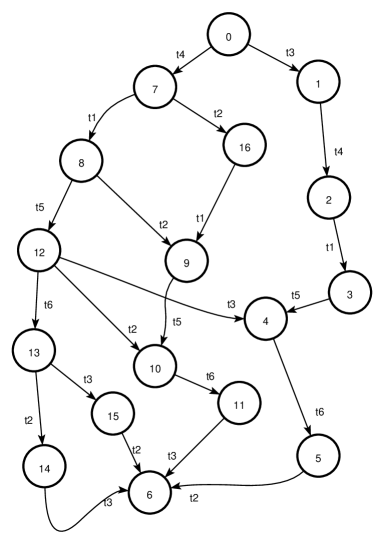
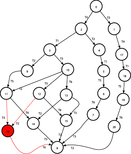
(a)	(b)

Figure 2: The exact graph and its DBM overapproximation of the $ITPN$ of Fig.1

To illustrate both graph constructions, let us consider again the net of Fig 1. The exact state class graph resulted after applying the algorithm of Definition 4 is shown in Fig. 2.a. Its DBM overapproximation resulted by the application of the algorithm given in Definition 5 is depicted in Fig. 2.b. Hence, the exact graph contains 17 classes and 22 edges, whereas its DBM overapproximated graph contains 21 classes and 28 edges. By comparing both graphs, we notice that the transition $t_{3}$ is firable from the class $\widetilde{E^{11}}$ in $\widetilde{GR},$ whereas it is not from $E^{10}$ in $GR$. Moreover, $t_{2}$ is firable from $\widetilde{E^{12}}$ whereas it is not from $E^{4}.$ The sequences added in the graph $\widetilde{GR}$ due to overapproximation are highlighted in red in Fig 2.b.

Although the cost of computing the DBM overapproximation is low comparing to the exact construction, it remains that in certain cases the approximation is too coarse to restore properties of interest and especially quantitative properties. In actual fact, more transitions remain persistently enabled along firing sequences more the approximation looses its precision and therefore includes false behaviors that skew the time analysis of the system. Besides, these false behaviors may compute an infinity of unreachable markings while the exact construction is indeed bounded. Hence, this prevents the DBM overapproximation to terminate while the exact construction may converge.

We investigate in the next section a new approach to compute a tighter DBM overapproximation. The idea is to restore from previous classes in the firing sequence time constraints that are used to tighten still more the DBM overapproximation of a class.

4 Time distance based Approximation of the ITPN State Space

$t_{f}^{1}$	$t_{f}^{2}$		$t_{f}^{n}$	fired transitions
0$<$——–$>$	1 $<$ ——–$>$2	$\ .\ .\ .$	n-1$<$——–$>$n	firing points
$M^{0}$	$M^{1}\qquad\ \ \ \ \ \ \ \ M^{2}$		$M^{n-1}$     $M^{n}$	reachable markings
$e^{0}$	$e^{1}$    $e^{2}$		$e^{n-1}$       $e^{n}$	reachable states
$t_{f}^{1}$	$t_{f}^{2}$		$t_{f}^{n}$	firing time distances

Let $RT:=(P,T,B,F,M^{0},I,IH)$ be an Inhibitor arc Time Petri Net. We suppose that a sequence of transitions $S=(t_{f}^{1},..,t_{f}^{n})$ has been fired in RT. The marking and the state reachable at the $(j)^{th}$ firing point are denoted $M^{j}$ and $e^{j}$ respectively.  Therefore, for the firing point $(n)$ we define the following:

• The marking reachable at point $(n)$ is denoted by $M^{n}$.

• The function $Ne^{n}:Te(M^{n})\longrightarrow\left\{0,1,..,n\right\};~{}Ne^{n}(t)$ gives, as shown in $Fig.3,$ the number of the firing point that has enabled the transition $t$ for the last time, provided that $t$ remains persistently enabled up to the firing point $(n)$. Thereafter, we denote by$~{}[Ne^{n}]$ the set of transition’s enabling points reported at the firing point $(n).$

• The function $Ni^{n}:Te(M^{n})\longrightarrow\left\{-1,0,1,..,n\right\}.~{}Ni^{n}(t)$ gives, as shown in $Fig.3,$ the number of the firing point that has inhibited the transition $t$ for the last time, provided that $t$ remains persistently enabled up to the firing point $(n)$. We have $Ni^{n}(t)=-1$ if $t$ has never been inhibited since its last enabling point. Thereafter, we denote by$~{}[Ni^{n}]$ the set of transition’s inhibiting points reported at the firing point $(n).$

• The function $Na^{n}:Te(M^{n})\longrightarrow\left\{-1,0,1,..,n\right\}.~{}Na^{n}(t)$ gives, as shown in $Fig.3,$ the number of the firing point that has activated the transition $t$ for the last time, provided that $t$ remains persistently enabled up to the firing point $(n)$. We have $Na^{n}(t)=-1$ if $t$ has never been activated since its last enabling point. Thereafter, we denote by$~{}[Na^{n}]$ the set of transition’s activating points reported at the firing point $(n).$

• We denote thereafter by $Point^{n}$ the set $[Ne^{n}]\cup[Ni^{n}]\cup[Na^{n}]-\{-1\}.$

Figure 3: Last enabling inhibiting and activating points of a transition.

Let us consider the firing of a sequence of transitions $S=\left(t_{f}^{1},..,t_{f}^{n}\right)$ in the graph $GR$. The sequence $S$ describes a path in the graph $GR$ going from the node representing the class $E^{0}$ to the node which represents the class $E^{n}$. We introduce next the time distance system that encodes the quantitative properties of some subsequences of $S$.

Definition 6

Let $E^{n}=(M^{n},D^{n})$ be a class reachable in $GR,$ after firing the sequence $S=\left(t_{f}^{{}_{1}},..,t_{f}^{n}\right).$ For point $(n),$ we define the time distance system, noted $DS^{n},$ as follows:
$DS^{n}=\left\{\begin{tabular}[]{l}{\Huge$\wedge$}${}_{\forall i\in Point^{n}},-DS^{n}[n,i]\leq\underline{t_{f}^{{}_{i+1}}}+..+\underline{t_{f}^{n}}\leq DS^{n}[i,n]$\newline \\ {\Huge$\wedge$}${}_{\forall i\in Point^{n}\cup\{n\}}${\Huge$\wedge$}${}_{\forall t\in Te(M^{n})},-DS^{n}[t,i]\leq\underline{t_{f}^{{}_{i+1}}}+..+\underline{t_{f}^{n}}+\underline{t}\leq DS^{n}[i,t]$\end{tabular}\right.$ 

More concretely, if $t$ is an enabled transition for $E^{n}$, then $DS^{n}[t,i]$ represents the opposite value of the minimum residual time of $t$ computed from the firing point $(i),$ whereas $DS^{n}[i,t]$ denotes its maximum residual time relatively to the firing point $(i)$. Moreover, $DS^{n}[i,n]$ (respectively, $DS^{n}[n,i]),$ denotes the maximum time distance (respectively, the opposite value of the minimum time distance), between the firing points $(i)$ and $(n)$. The coefficients of the system $DS^{0}$ are defined as follows: We have $Point^{n}=\{0\};$
$\forall t\in Te(M^{0}),$   $DS^{0}[0,0]=0,$ $DS^{0}[0,t]=tmax(t),$ $DS^{0}[t,0]=-tmin(t).$       

Thereafter, we encode the system $DS^{n}$ as four matrices. For instance, the coefficients of the system $DS^{0}$ of the $ITPN$ of Fig.1 are given in Tab.2.

Table 2: The time distance system at firing point $(0)$

$DS^{0}[i,t]$ $t_{1}$ $t_{3}$ $t_{4}$ $0$ 3 4 2   $DS^{0}[t,i]$ $t_{1}$ $t_{3}$ $t_{4}$ $0$ -3 -2 0   $DS^{0}[i,n]$ $0$ $0$ 0 $DS^{0}[n,i]$ $0$ $0$ 0

Next definition shows how the system $DS^{n}$ can be determined recursively as a result of solving a general polyhedral system.

Definition 7

Let $E^{n-1}=(M^{n-1},D^{n-1})$ be a class reachable in $GR$ and let $\mathit{DS}^{n-1}$ be the time distance system associated with the class $E^{n-1}$. Let us consider $E^{n}=(M^{n},D^{n})$ be the class reachable from $E^{n-1}$ after firing the transition $t_{f}^{n}$. The time distance system $DS^{n}$ associated with $E^{n}$ can be worked out recursively from the systems $DS^{n-1},D^{n-1}$  as follows:

1. Compute the function $Ne$ ⁿ as follows: $\forall t\in Te(M^{n})$
    If $t\in New(M^{n})$ then $Ne^{n}(t):=n$   else $Ne^{n}(t):=Ne^{n-1}(t).$
   Compute the function $Ni$ⁿ as follows:
   If $Ne^{n}(t)=n$ then if $t\in Ti(M$${}^{n})$ then $Ni^{n}(t):=n$ else $Ni^{n}(t):=-1.$  

   else if $t\in Ta(M$ ${}^{n-1})$ $\wedge t\in Ti(M$${}^{n})$ then $Ni^{n}(t):=n.$

   else $Ni^{n}(t):=Ni^{n-1}(t)$.
   Compute the function $Na$ⁿ as follows:
   If $Ne^{n}(t)=n$ then if $t\in Ta(M$${}^{n})$ then $Na^{n}(t):=n$ else $Na^{n}(t):=-1.$  

   else if $t\in Ta(M$${}^{n})$$\wedge t\in Ti(M$${}^{n-1})$ then $Na^{n}(t):=n.$

   else $Na^{n}(t):=Na^{n-1}(t)$.
   

2. Augment the system $D^{n-1}$ with the firing constraints of $t_{f}^{n}$ that we write $D_{a}^{n-1}=$ $D_{a}^{n-1}\wedge(\forall t\in Ta(M^{n-1}),\quad\underline{t_{{}^{f}}^{n}}\leq\underline{t})$

3. In the system $D_{a}^{n-1}\wedge DS^{n-1}$ rename each variable $\underline{t}$ related to an activated transition which is persistent for Mⁿ with $\underline{t}^{\prime}+\underline{t_{f}^{n}}$. For inhibited transitions, rename the related variable $\underline{t}$ with $\underline{t}^{\prime}$.

4. In the resulted system and by intersection of the constraints, remove the variables related to disabled transitions and determine the constraints of $DS^{n}$.  

5. In the obtained system, add constraints related to newly enabled transitions, as follows : $\forall t\in New(M^{n}),$ $\forall i\in Point^{n}\cup\{n\}$
   $-DS^{n}[n,i]-tmin(t)\leq\underline{t_{f}^{{}_{i+1}}}+..+\underline{t_{f}^{n}}+\underline{t}\leq DS^{n}[i,n]+tmax(t).$

The computation of the system $DS^{n}$ is very complex as it needs at each step to manipulate a global system which may contain polyhedral constraints. Concretely, if the latter appears in $D^{n-1}$ then the cost of computing $DS^{n}$ is exponential on the number of variables, otherwise it is polynomial. However, in most of the cases, polyhedral constraints do not affect the computation of the time distances. Therefore, to alleviate the computation effort, the idea is to leave out systematically such constraints during the process (keeping only the $DBM$ system to represent the space of the class $E^{n-1}),$ with a risk however to compute in certain cases an overapproximation of the system $DS^{n}.$ The resulted system obtained by DBM restriction is noted thereafter $\widetilde{DS^{n}}$ and we have $\widetilde{DS^{0}}=DS^{0}$. The next proposition provides an algorithm to compute recursively and efficiently the coefficients of the system $\widetilde{DS_{n}}$ in the context of the DBM overapproximated graph that we aim to compute, noted $\widetilde{GRc}$. However the same algorithm can be applied in the context of the exact graph $GR$ while restricting the system $D$ to $\overrightarrow{D}$ ( $\overrightarrow{D}$ is the tightest DBM overapproximation that one can compute from $D$).

Proposition 1

Let the graph $\widetilde{{\small{GRc}}}$ be a DBM overapproximation of the graph ${\small GR}$. Let $\widetilde{{\small{E}}_{{\small{c}}}^{{\small{n-1}}}}$$=(M^{n-1},\widetilde{D_{c}^{n-1}})$ be a class reachable in $\widetilde{{\small{GRc}}}$, from the initial class after firing the sequence $S=\left(t_{f}^{{}_{1}},..,t_{f}^{n-1}\right)$. Let $\widetilde{\mathit{DS}^{n-1}}$ be the DBM overapproximated time distance system associated with the class $\widetilde{{\small{E}}_{{\small{c}}}^{{\small{n-1}}}}$. Let us consider $\widetilde{{\small{E}}_{{\small{c}}}^{{\small{n}}}}$$=(M^{n},\widetilde{{D}_{{c}}^{{n}}})$ the class reachable from $\widetilde{{\small{E}}_{{\small{c}}}^{{\small{n-1}}}}$ after firing the transition $t_{f}^{n}$. The DBM overapproximated time distance system $\widetilde{{\small{DS^{n}}}}$ associated with $\widetilde{{\small{E}}_{{\small{c}}}^{{\small{n}}}}$ can be computed recursively from previous systems in the sequence $\mathit{S}$, as follows:  

• Compute the function $Ne^{n},Ni^{n}$ and $Na^{n}$ as in Definition.7.

• The coefficients of the system $\widetilde{DS^{n}}$ are computed by using the following formulae:

  $\forall i\in Point$ⁿ 

  $\quad\widetilde{DS^{n}}[i,n]:=\lambda^{n-1}[i];$

  $\quad\widetilde{DS^{n}}[n,i]:=\widetilde{DS^{n-1}}[t_{f}^{n},i];$

  $\quad\widetilde{DS^{n}}[n,n]:=0;$

  such that $\forall i\in Point^{n}\cup\{n\},$ $\lambda^{n}[i]=\underset{t\in Ta(M^{n})}{MIN}\left\{\widetilde{DS^{n}}[i,t]\right\}$ 

  $\forall t\in Te(M^{n}),$ $\forall i\in Point$ⁿ

  If $Ne^{n}(t)=n$ ($t$ is newly enabled)

            $\widetilde{DS^{n}}[i,t]:=\widetilde{DS^{n}}[i,n]+tmax(t);$ $\quad\widetilde{DS^{n}}[t,i]:=\widetilde{DS^{n}}[n,i]-tmin(t);$ $\widetilde{DS^{n}}[n,t]:=tmax(t);$ $\quad\widetilde{DS^{n}}[t,n]:=-tmin(t);$                 
  

  If $Ne^{n}(t)\neq n$ ($t$ is persistent)

  If $t\notin Ti(M^{n-1})$ $\ (t$ is not inhibited for $M$^n-1), 

  Let ${\scriptsize{\small r=Ne}}^{{\scriptsize{\small n}}}{\scriptsize{\small(t),s=Ni}}^{{\scriptsize{\small n-1}}}{\scriptsize{\small(t)}}$ and ${\scriptsize{\small p=Na}}^{{\scriptsize{\small n}}}{\scriptsize{\small(t).}}$ 

  $\quad\quad\quad\widetilde{DS^{n}}[i,t]:=MIN\left(\begin{tabular}[]{l}$\left\{\begin{tabular}[]{ll}$\widetilde{DS^{s}}[i,t]+\lambda^{n-1}[s]+\widetilde{DS^{n}}[n,p]$&if $0\leq i\leq s\leq p$\\ $\widetilde{DS^{i}}[i,t]+\widetilde{DS^{n}}[i,n]+\widetilde{DS^{n}}[n,p]$&if $0\leq s\leq i\leq p$\end{tabular}\right.$\\ $\widetilde{DS^{n-1}}[i,t]$\\ $\widetilde{DS^{n}}[i,n]+\widetilde{DS^{n-1}}[n-1,t]+\widetilde{DS^{n-1}}[t_{f}^{n},n-1]$\end{tabular}\right.$
  

  $\quad\quad\quad\widetilde{DS^{n}}[t,i]:=MIN\left(\begin{tabular}[]{l}$\left\{\begin{tabular}[]{ll}$\widetilde{DS^{s}}[t,i]+\widetilde{DS^{n-1}}[t_{f}^{n},s]+\widetilde{DS^{n}}[p,n]$&if $0\leq i\leq s\leq p$\\ $\widetilde{DS^{i}}[t,i]+\widetilde{DS^{n}}[n,i]+\widetilde{DS^{n}}[p,n]$&if $0\leq s\leq i\leq p$\end{tabular}\right.$\\ $\widetilde{DS^{n-1}}[t,i]$$\quad$\\ $\widetilde{DS^{n}}[n,i]+MIN(0,$ $\widetilde{DS^{n-1}}[t,n-1]+\lambda^{n-1}[n-1])$\end{tabular}\right.$

  $\quad\quad\quad\widetilde{DS^{n}}[t,n]:=\quad MIN\left\{\begin{tabular}[]{l}$\widetilde{\beta_{c}^{n-1}}[t]$\\ $MIN(0,$ $\widetilde{DS^{n}}[t,r]+\widetilde{DS^{n}}[r,n])$\end{tabular}\right.;$

  $\quad\quad\quad\widetilde{DS^{n}}[n,t]:=\quad MIN\left\{\begin{tabular}[]{l}$\widetilde{D_{c}^{n-1}}[t_{f}^{n},t]$\\ $\widetilde{DS^{n}}[r,t]+\widetilde{DS^{n}}[n,r]$\end{tabular}\right.;\vskip 3.0pt plus 1.0pt minus 1.0pt$

        If $t\in Ti(M^{n-1})$ $\ (t$ is inhibited for $M$^n-1),

              Let $s=Ni^{n}(t)$ and $r=Ne^{n}(t).$

        $\quad\widetilde{DS^{n}}[i,t]:=$

  $\quad\quad\quad\quad MIN$$\left(\begin{tabular}[]{l}$\left\{\begin{tabular}[]{ll}$\widetilde{DS^{s}}[i,t]+\widetilde{DS^{n}}[s,n]$&if $i\leq s$\\ $\widetilde{DS^{i}}[i,t]+\widetilde{DS^{n}}[i,n]$&if $s\leq i$\end{tabular}\right.\vskip 3.0pt plus 1.0pt minus 1.0pt$\\ $\widetilde{DS^{n-1}}[i,t]+\lambda^{n-1}[n-1]$\end{tabular}\right.$

     $\quad\quad\widetilde{DS^{n}}[t,i]:=$

  $\quad\quad\quad\quad MIN$$\left(\begin{tabular}[]{l}$\left\{\begin{tabular}[]{ll}$\widetilde{DS^{s}}[t,i]+\widetilde{DS^{n}}[n,s]$&if $i\leq s$\\ $\widetilde{DS^{i}}[t,i]+\widetilde{DS^{n}}[n,i]$&if $s\leq i$\end{tabular}\right.\vskip 3.0pt plus 1.0pt minus 1.0pt$\\ $\widetilde{DS^{n-1}}[t,i]+\widetilde{DS^{n-1}}[t_{f}^{n},n-1]$\end{tabular}\right.$

        $\quad\widetilde{DS^{n}}[n,t]:=\quad MIN\left(\begin{tabular}[]{l}$\widetilde{DS^{n}}[r,t]+$$\widetilde{DS^{n}}[n,r]$\\ $\widetilde{DS^{n-1}}[n-1,t]$\\ $\widetilde{D^{n-1}}[t_{f}^{n},t]+$$\lambda^{n-1}[n-1];$\end{tabular}\right.$

           $\widetilde{DS^{n}}[t,n]:=\quad MIN\left(\begin{tabular}[]{l}$MIN(0,\widetilde{DS^{n}}[t,r]+\widetilde{DS^{n}}[r,n])$\\ $\widetilde{DS^{n-1}}[t,n-1]$\\ $\widetilde{DS^{n-1}}[t_{f}^{n},n-1]+\widetilde{\beta_{c}^{n-1}}[t]$\end{tabular}\right.\vskip 6.0pt plus 2.0pt minus 2.0pt$

  such that $\forall t\in Te(M^{n-1}),\quad\widetilde{\beta_{c}^{n-1}}[t]=\underset{\forall t^{\prime}\in Ta(M^{n-1})}{MIN}\left\{\widetilde{D_{c}^{n-1}}[t,t^{\prime}]\right\}.$

The previous proposition provides an efficient algorithm to compute an overapproximation of the system $DS^{n}.$ For this effect, the algorithm starts to determine the set $Point^{n}$. Then it calculates the coefficients $\widetilde{DS^{n}}[i,n]$ and $\widetilde{DS^{n}}[n,i]$ for each point $i\in Point^{{\small n}}$. Then for each enabled transition $t$, the algorithm computes the other coefficients following the cases:

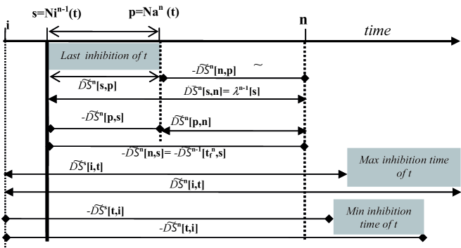
(a)

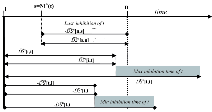
(b)

Figure 4: Time distance Computation.

• When dealing with newly enabled transitions, the formulae are obvious and are the same for inhibited and activated transitions.

• When handling persistent transitions, the algorithm proceeds first to compute the distances $\widetilde{DS^{n}}[i,t]$ and $\widetilde{DS^{n}}[t,i]$ for each point $i\in Point^{{\small n}}$. It is noteworthy that the previous distances are more likely to maintain their values along a firing sequence as long as $t$ is not inhibited in the sequence. However, if $t$ becomes inhibited then these distances increase by the time elapsed during its inhibition. Therefore, if a transition is activated for the point $(n-1)$, and $t$ has never been inhibited since its last enabling point ($s=-1$), then both distances are more likely to maintain their old values, even decreasing in very rare cases if there is state space restriction (see the last two items of the MIN). However, if the transition $t$ has been inhibited at least once since its last enabling point ($s\geq 0$), then the duration of its last inhibition time should be re-calculated at each new reachable point to better approximate these distances. In actual fact, because of space restriction the inhibition times of $t$ may decrease even after that $t$ has been activated. As a result, the interval $[-\widetilde{DS^{n}}[t,i],\widetilde{DS^{n}}[i,t]]$ may only narrow along a firing sequence as long as $t$ remains activated. For this purpose, we need to restore some time information computed earlier in the sequence at points ($s$) and ($i$). For instance, if the point $(i)$ occurs first in the firing sequence, then the distance $\widetilde{DS^{n}}[i,t]$ is likely to be equal to the same distance computed at point $s$, $\widetilde{DS^{s}}[i,t]$ augmented with the maximal inhibition time of $t$, namely $\lambda^{n-1}[s]+\widetilde{DS^{n}}[n,p]$ (see Fig 3.a,). Otherwise, if the point $(i)$ occurs during the inhibition time of $t$, then the distance $\widetilde{DS^{n}}[i,t]$ is likely to be equal to the same distance computed at point $(i),$ $\widetilde{DS^{i}}[i,t]$ augmented with the maximal inhibition time of $t$ from point $(i)$ to $(p):\widetilde{DS^{n}}[i,n]+\widetilde{DS^{n}}[n,p]$.

  In case that $t$ is inhibited for the point $(n-1)$, we follow the same approach as previously to compute the same distances. However, in this case the adjustment of the approximation is carried out during the inhibition time of the transition $t$. At each new firing point, the residual time of an inhibited transition should increase with the dwelling time measured at point $(n-1)$. Furthermore, as shown in Fig 3.b, if $i$ occurs before $s$, then this distance should not surpass the residual time of the transition reported at point $(s)$ augmented with the inhibition time elapsed from $(s)$ till the current point $(n)$.

• The algorithm ends the process by calculating the coefficients $\widetilde{DS^{n}}[n,t]$ and $\widetilde{DS^{n}}[t,n]$. As these coefficients denote the same distances as respectively $\widetilde{D_{c}^{n}}[\bullet,t]$ and $\widetilde{D_{c}^{n}}[\bullet,t]$ already defined in a classical $DBM$ system. Therefore, their computation is worked out also by using the formulae of Definition 5, already established in [16]. Better still, new formulae are added to tighten still more their approximation.

We propose thereafter to exploit the time distance system in the computation of an overapproximation of the state class graph of an$\ ITPN$.  The proposition.1 shows that by overapproximating the computation of the system $DS^{n},$ we reduce the effort of its computation to a polynomial time. From this system, we are able to restore some time information that makes it possible to compute a $DBM$ overapproximation that is tighter than that of other approaches [16][5][9]. Formally, the time distance based approximation of the graph $GR$ is built as follows:

Definition 8

The time distance based approximation graph of an $ITPN$, denoted by $\widetilde{GRc}$ is the tuple $(\widetilde{CEc},\widetilde{E_{c}^{0}},\leadsto)$ such that:

• $\widetilde{CEc}$ is the set of approximated classes reachable in $\widetilde{GRc\text{ }};$ 

• $\widetilde{E_{c}^{0}}=(M^{0},Ne^{0},Ni^{0},Na^{0},\widetilde{DS^{0}},\widetilde{D_{c}^{0}})\in\widetilde{CEc}$ is the initial class such that $\widetilde{{DS}}$${}^{0}=DS^{0}$ and $\widetilde{{D_{c}^{0}}}$ is the system $\forall t,t^{\prime}\in Te(M^{0}),\underline{t}^{\prime}-\underline{t}\leq tmax(t^{\prime})-tmin(t)$

• $\leadsto$ is a transition relation between approximated classes defined on $\widetilde{CEc}\times T\times\widetilde{CEc},$ such that $((M^{n-1},Ne^{n-1},Ni^{n-1},Na^{n-1},\widetilde{DS^{n-1}},\widetilde{D_{c}^{n-1}}),t_{f}^{n},(M^{n},Ne^{n},Ni^{n},Na^{n},\widetilde{DS^{n}},\widetilde{D_{c}^{n}}))$ $\ \in\leadsto,$ iff:

  (i)

  $t_{f}^{n}$$\in Ta(M^{n-1}).$

  (ii)

  $\widetilde{\beta_{c}^{n-1}}[t_{f}^{n}]\geq 0$.

  The new class is computed as follows:

  • $\forall p\in P,$ $M^{n}(p):=M^{n-1}(p)-B(p,t_{f}^{n})+F(p,t_{f}^{n})\vskip 3.0pt plus 1.0pt minus 1.0pt.$

  • Compute the function $Ne^{n},Ni$ⁿ and $Na^{n}$ as in Definition.7.

  • Compute the coefficients of the system $\widetilde{DS^{n}}$ as in Proposition 1:

  • The DBM system $\widetilde{D_{c}^{n}}$ is obtained as follows :

    $\forall(t,t^{\prime})\in(Te(M^{n-1}))^{2}\wedge(t\neq t^{\prime})$

    If $t$ or $t^{\prime}$ are newly enabled.

    $\ \ \quad\widetilde{D_{c}^{n}}[t,t^{\prime}]:=\widetilde{DS^{n}}[n,t^{\prime}]+\widetilde{DS^{n}}[t,n]$.

    If $t$ and $t^{\prime}$ are persistent.

        If ($t,t^{\prime})\notin(Ti(M^{n-1}))^{2}$  ($t$ and $t^{\prime}$ are not inhibited for $M^{n-1}$)

    $\quad\quad\quad\widetilde{D_{c}^{n}}[t,t^{\prime}]:=MIN(\widetilde{D_{c}^{n-1}}[t,t^{\prime}],\quad\alpha^{n}[t,t^{\prime}]).\vskip 6.0pt plus 2.0pt minus 2.0pt$ 

        If  ($t$,$t^{\prime})\in(Ti(M^{n-1}))^{2}$  ($t$ and $t^{\prime}$ are inhibited for $M^{n-1}$)

    $\quad\quad\quad\widetilde{D_{c}^{n}}[t,t^{\prime}]:=MIN(\widetilde{D_{c}^{n-1}}[t,t^{\prime}],\quad\alpha^{n}[t,t^{\prime}]).\vskip 6.0pt plus 2.0pt minus 2.0pt$ 

        If $\ (t\in Ti(M^{n-1}))\wedge(t^{\prime}\notin Ti(M^{n-1}))$    (Only $t$ is inhibited for $M^{n-1}$).

    $\quad\quad\quad\widetilde{D_{c}^{n}}[t,t^{\prime}]$ $:=MIN(\widetilde{D_{c}^{n}}[t,t^{\prime}]+\widetilde{D_{c}^{n-1}}[t_{f}^{n},\bullet],\quad\alpha^{n}[t,t^{\prime}]).$ 

        If $\ (t\notin Ti(M^{n-1}))\wedge(t^{\prime}\in Ti(M^{n-1}))$    (Only $t^{\prime}$ is inhibited for $M^{n-1}$)

    $\quad\quad\quad\widetilde{D_{c}^{n}}[t,t^{\prime}]$ $:=$$MIN(\widetilde{D_{c}^{n-1}}[t,t^{\prime}]+\lambda^{n-1}[n-1],\quad\alpha^{n}[t,t^{\prime}]).$

    such that $\alpha^{n}[t,t^{\prime}]$ =$\underset{i\in Point^{n}\cup\{n\}}{MIN}\left(\widetilde{DS^{n}}[i,t^{\prime}]+\widetilde{DS^{n}}[t,i]\right)$

The previous definition provides an algorithm to compute a DBM overapproximation of an ITPN. To avoid redundancy, each computed DBM system of a reachable class, noted $\widetilde{D_{c}^{n}},$ is reduced to the constraints $t^{\prime}-t\leq\widetilde{D_{c}^{n}}[t,t^{\prime}].$ Note that the other constraints of type $-\widetilde{D_{c}^{n}}[t,\bullet]\leq t\leq\widetilde{D_{c}^{n}}[\bullet,t]$ are already computed in the system $\widetilde{DS^{n}}$ as $-\widetilde{DS^{n}}[t,n]\leq t\leq\widetilde{DS^{n}}[n,t].$ Comparatively to the construction of the graph $\widetilde{GR}$ given in Definition.5, the class is extended to the parameters $Ni^{n}$, $Na^{n}$, $Ni^{n}$ and $\widetilde{DS^{n}}$. The DBM system $\widetilde{D_{c}^{n}}$ computed thereof is used in the firing and class’ equivalence tests. It is noteworthy that the same firing condition is used in both constructions. However, the computation of the coefficients of $\widetilde{D_{c}^{n}}$ are better approximated than those of the system $\widetilde{D^{n}}$. First of all, as it is given in Proposition 1, the maximal and the minimal residual times of an enabled transition use formulae that are more precise than those provided in Definition 5. As a result, the DBM coefficients $\widetilde{D_{c}^{n}}[t,t^{\prime}]$ are more precise too. This makes it possible to tighten still more the approximation and therefore to avoid the generation of additional sequences that stand in the graph $\widetilde{GR}$. The resulted graph $\widetilde{GRc}$ is therefore more precise than $\widetilde{GR}$. However, the cost of computing the system $\widetilde{D_{c}^{n}}$ is slightly higher than $\widetilde{D^{n}}$ as it requires also to consider the computation effort of the system $\widetilde{DS^{n}}$. Nevertheless, the total cost of computing a class in $\widetilde{GRc}$ remains polynomial and equal to $o(m^{2}l+m^{2}+ml),$ where $m$ and $l$ denote respectively the number of enabled transitions and the number of reported points. We need to prove now formally that the construction of the $\widetilde{GRc}$ computes in all cases an overapproximation of the exact graph $GR,$ which remains always tighter than the graph $\widetilde{GR}$.

Theorem 1

Let $RT$ be an ITPN and $\widetilde{GR}=(\widetilde{CE},(M^{0},\widetilde{D^{0}}),\rightsquigarrow),$ $\widetilde{GRc}=(\widetilde{CEc},(M^{0},Ne^{0},Ni^{0},Na^{0},\widetilde{DS^{0}},\widetilde{D_{c}^{0}}),\leadsto)$ and $GR=(CE,(M^{0},D^{0}),\longmapsto)$ the graphs build on $RT$: $\widetilde{GR}$ is an overapproximation of the graph $\widetilde{GRc}$ and the latter is an overapproximation of the exact graph $GR$.

[Proof.] The proof is given in Appendix.

The previous theorem establishes that the algorithm of $Definition.8$ computes a more precise graph than that computed by using other $DBM$ overapproximation approaches [16][9][5]. As a result, the size of the graph is reduced since additional sequences might be fired when using classical DBM approximations whereas they are not in $\widetilde{GRc}$ as well as in $GR$. To advocate the benefits of the defined construction, let us consider again the $ITPN$ of Fig 1. As shown in Fig.5, the obtained graph $\widetilde{GRc}$ is much compact than $\widetilde{GR}$ and contains $19$ classes and $25$ edges. Moreover, some of the additional sequences reported in $\widetilde{GR}$ due to overapproximation are removed in $\widetilde{GRc}.$

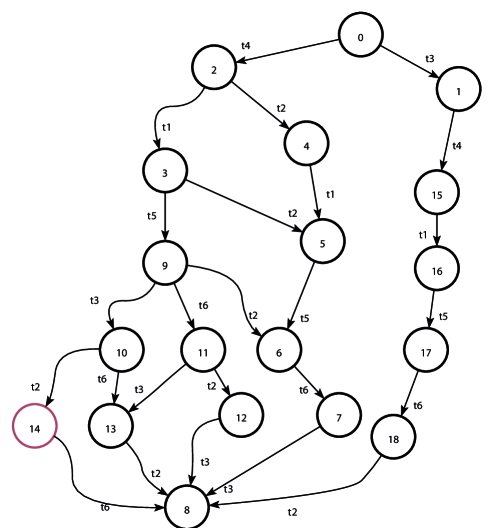
Figure 5: Time Distance based approximation graph.

For example, let us consider the firing sequence $\widetilde{E_{c}^{0}}\overset{t_{4}}{\leadsto}\widetilde{E_{c}^{2}}\overset{t_{1}}{\leadsto}$ $\widetilde{E_{c}^{3}}\overset{t_{2}}{\leadsto}$ $\widetilde{E_{c}^{5}}\overset{t_{5}}{\leadsto}\widetilde{E_{c}^{6}}$ already discussed in page 10. After firing the transition $t_{4}$ from the initial class, we reach the class $\widetilde{E_{c}^{2}}$ where $t_{3}$ is inhibited for the first time. The algorithm proceeds first by computing the system $\widetilde{DS^{2}}$ from $\widetilde{DS^{0}}$ and $\widetilde{D_{c}^{0}},$ then it determines the system $\widetilde{D_{c}^{2}}$.

$\widetilde{E_{c}^{2}}$=$\left(\begin{tabular}[]{lll}\lx@intercol\begin{tabular}[]{ll}$M^{2}:p_{2},p_{3},p_{3},p_{7}\rightarrow 1$&$Ni^{2}$: $\{t_{1},t_{2},t_{7}\}\rightarrow-1;t_{3}\rightarrow 2.$\\ $Ne^{2}$: $\{t_{1},t_{3}\}\rightarrow 0;\{t_{2},t_{7}\}\rightarrow 2.$&$Na^{2}$: $\{t_{7},t_{2}\}\rightarrow 2;t_{3}\rightarrow 0;t_{1}\rightarrow 0.$\end{tabular}\hfil\lx@intercol \\ \begin{tabular}[]{|c|c|c|c|c|}\hline\cr$\widetilde{D_{c}^{2}}$&$t_{1}$&$t_{2}$&$t_{3}$&$t_{7}$\\ \hline\cr$t_{1}$&0&4&1&9\\ \hline\cr$t_{2}$&1&0&2&8\\ \hline\cr$t_{3}$&1&5&0&10\\ \hline\cr$t_{7}$&-7&-5&-6&0\\ \hline\cr\end{tabular}&\begin{tabular}[]{l}\begin{tabular}[]{|c|c|c|c|c|}\hline\cr$\widetilde{DS^{2}}[i,t]$&$t_{1}$&$t_{2}$&$t_{3}$&$t_{7}$\\ \hline\cr{\tiny 0}&{\tiny 3}&{\tiny 7}&{\tiny 4}&{\tiny 12}\\ \hline\cr n={\tiny 2}&{\tiny 3}&{\tiny 5}&{\tiny 4}&{\tiny 10}\\ \hline\cr\end{tabular}\vskip 6.0pt plus 2.0pt minus 2.0pt\\ \begin{tabular}[]{|c|c|c|c|c|}\hline\cr$\widetilde{DS^{2}}[t,i]$&$t_{1}$&$t_{2}$&$t_{3}$&$t_{7}$\\ \hline\cr{\tiny 0}&{\tiny-3}&{\tiny-2}&{\tiny-2}&{\tiny-10}\\ \hline\cr n={\tiny 2}&{\tiny-1}&{\tiny-2}&{\tiny 0}&{\tiny-10}\\ \hline\cr\end{tabular}\vskip 6.0pt plus 2.0pt minus 2.0pt\end{tabular}\vskip 6.0pt plus 2.0pt minus 2.0pt&\ \begin{tabular}[]{l}\begin{tabular}[]{|c|c|}\hline\cr$\widetilde{DS^{2}}[i,n]$&{\tiny 0}\\ \hline\cr n=2&{\tiny 2}\\ \hline\cr\end{tabular}\vskip 6.0pt plus 2.0pt minus 2.0pt\\ \begin{tabular}[]{|c|c|}\hline\cr$\widetilde{DS^{2}}[n,i]$&{\tiny 0}\\ \hline\cr n=2&{\tiny 0}\\ \hline\cr\end{tabular}\vskip 6.0pt plus 2.0pt minus 2.0pt\end{tabular}\end{tabular}\right.$

Then firing $t_{1}$ from $\widetilde{E_{c}^{2}}$ yields the class $\widetilde{E_{c}^{3}}$. At this stage, the resulted DBM system $\widetilde{D_{c}^{2}}$ is equal to that obtained in the graph $\widetilde{GR}$ after firing the same sequence.

$\widetilde{E_{c}^{3}}$=$\left(\begin{tabular}[]{lll}\lx@intercol\begin{tabular}[]{ll}$M^{3}:p_{2},p_{3},p_{5},p_{7}\rightarrow 1$&$Ni^{3}$: $\{t_{2},t_{5},t_{7}\}\rightarrow-1;t_{3}\rightarrow 2.$\\ $Ne^{3}$: $\{t_{2},t_{7}\}\rightarrow 2;t_{3}\rightarrow 0;t_{5}\rightarrow 3.$&$Na^{3}$: $\{t_{7},t_{2}\}\rightarrow 2;t_{3}\rightarrow 0;t_{5}\rightarrow 3.$\end{tabular}\hfil\lx@intercol \\ \begin{tabular}[]{|c|c|c|c|c|}\hline\cr$\widetilde{D_{c}^{3}}$&$t_{2}$&$t_{3}$&$t_{5}$&$t_{7}$\\ \hline\cr$t_{2}$&0&4&0&8\\ \hline\cr$t_{3}$&4&0&0&9\\ \hline\cr$t_{5}$&4&4&0&9\\ \hline\cr$t_{7}$&-5&-3&-7&0\\ \hline\cr\end{tabular}\vskip 6.0pt plus 2.0pt minus 2.0pt&\begin{tabular}[]{l}\begin{tabular}[]{|c|c|c|c|c|}\hline\cr$\widetilde{DS^{3}}[i,t]$&$t_{2}$&$t_{3}$&$t_{5}$&$t_{7}$\\ \hline\cr{\tiny 0}&{\tiny 7}&{\tiny 7}&{\tiny 3}&{\tiny 12}\\ \hline\cr{\tiny 2}&{\tiny 5}&{\tiny 7}&{\tiny 3}&{\tiny 10}\\ \hline\cr n={\tiny 3}&{\tiny 4}&{\tiny 4}&{\tiny 0}&{\tiny 9}\\ \hline\cr\end{tabular}\vskip 6.0pt plus 2.0pt minus 2.0pt\\ \begin{tabular}[]{|c|c|c|c|c|}\hline\cr$\widetilde{DS^{3}}[t,i]$&$t_{2}$&$t_{3}$&$t_{5}$&$t_{7}$\\ \hline\cr{\tiny 0}&{\tiny-3}&{\tiny-3}&{\tiny-3}&{\tiny-10}\\ \hline\cr{\tiny 2}&{\tiny-2}&{\tiny-1}&{\tiny-1}&{\tiny-10}\\ \hline\cr n={\tiny 3}&{\tiny 0}&{\tiny 0}&{\tiny 0}&{\tiny-7}\\ \hline\cr\end{tabular}\vskip 6.0pt plus 2.0pt minus 2.0pt\end{tabular}&\ \begin{tabular}[]{l}\begin{tabular}[]{|c|c|c|}\hline\cr$\widetilde{DS^{3}}[i,n]$&{\tiny 0}&{\tiny 2}\\ \hline\cr n=3&{\tiny 3}&{\tiny 3}\\ \hline\cr\end{tabular}\vskip 6.0pt plus 2.0pt minus 2.0pt\\ \begin{tabular}[]{|c|c|c|}\hline\cr$\widetilde{DS^{3}}[n,i]$&{\tiny 0}&{\tiny 2}\\ \hline\cr n=3&{\tiny-3}&{\tiny-1}\\ \hline\cr\end{tabular}\vskip 6.0pt plus 2.0pt minus 2.0pt\end{tabular}\end{tabular}\right.$

Firing the transition $t_{2}$ from the previous class leads to $\widetilde{E_{c}^{5}}$. Here, we notice that the minimal residual time of the persistent inhibited transition $t_{3}$ relatively to the point $(0)$ has increased to 4, as we have $\widetilde{DS^{5}}[t_{3},0]=-4.$ $\widetilde{\mathit{E}_{\mathit{c}}^{5}}$=$\left(\begin{tabular}[]{lll}\lx@intercol\begin{tabular}[]{ll}$M^{5}:p_{3},p_{5},p_{7}\rightarrow 1$&$Ni^{5}$: $\{t_{5},t_{7}\}\rightarrow-1;t_{3}\rightarrow 2.$\\ $Ne^{5}$: $t_{7}\rightarrow 2;t_{3}\rightarrow 0;t_{5}\rightarrow 3.$&$Na^{5}$: $t_{7}\rightarrow 2;t_{3}\rightarrow 0;t_{5}\rightarrow 3.$\end{tabular}\hfil\lx@intercol \\ \begin{tabular}[]{|c|c|c|c|}\hline\cr$\widetilde{D_{c}^{5}}$&$t_{3}$&$t_{5}$&$t_{7}$\\ \hline\cr$t_{3}$&0&-1&7\\ \hline\cr$t_{5}$&4&0&8\\ \hline\cr$t_{7}$&-3&-7&0\\ \hline\cr\end{tabular}\vskip 6.0pt plus 2.0pt minus 2.0pt&\vskip 6.0pt plus 2.0pt minus 2.0pt\begin{tabular}[]{l}\begin{tabular}[]{|c|c|c|c|}\hline\cr$\widetilde{DS^{5}}[i,t]$&$t_{3}$&$t_{5}$&$t_{7}$\\ \hline\cr{\tiny 0}&{\tiny 7}&{\tiny 3}&{\tiny 11}\\ \hline\cr{\tiny 2}&{\tiny 7}&{\tiny 3}&{\tiny 10}\\ \hline\cr 3&4&0&8\\ \hline\cr n={\tiny 5}&{\tiny 4}&{\tiny 0}&{\tiny 8}\\ \hline\cr\end{tabular}\vskip 3.0pt plus 1.0pt minus 1.0pt\\ \begin{tabular}[]{|c|c|c|c|}\hline\cr$\widetilde{DS^{5}}[t,i]$&$t_{3}$&$t_{5}$&$t_{7}$\\ \hline\cr{\tiny 0}&{\tiny-4}&{\tiny-3}&{\tiny-10}\\ \hline\cr{\tiny 2}&{\tiny-2}&{\tiny-2}&{\tiny-10}\\ \hline\cr 3&0&0&-7\\ \hline\cr n={\tiny 5}&{\tiny-1}&{\tiny 0}&{\tiny-7}\\ \hline\cr\end{tabular}\vskip 6.0pt plus 2.0pt minus 2.0pt\end{tabular}&\ \begin{tabular}[]{l}\begin{tabular}[]{|c|c|c|c|}\hline\cr$\widetilde{DS^{5}}[i,n]$&{\tiny 0}&{\tiny 2}&3\\ \hline\cr n=5&{\tiny 3}&{\tiny 3}&0\\ \hline\cr\end{tabular}\vskip 6.0pt plus 2.0pt minus 2.0pt\\ \begin{tabular}[]{|c|c|c|c|}\hline\cr$\widetilde{DS^{5}}[n,i]$&{\tiny 0}&{\tiny 2}&3\\ \hline\cr n=5&{\tiny-3}&{\tiny-2}&0\\ \hline\cr\end{tabular}\vskip 6.0pt plus 2.0pt minus 2.0pt\end{tabular}\end{tabular}\right.$

The formula given in Proposition 1 suggests to compute this distance from the system $\widetilde{DS^{2}}$, since $2$ is the point that inhibited $t_{3}$ for the last time. As $t_{3}$ still remains inhibited in the sequence we have according to Proposition 1, $\widetilde{DS^{5}}[t_{3},0]=MIN(\widetilde{DS^{2}}[t_{3},0]+\widetilde{DS^{5}}[2,5],$     $\widetilde{DS^{3}}[t_{3},0]+\widetilde{DS^{3}}[t_{2},3])$; we obtain $\widetilde{DS^{5}}[t_{3},0]=MIN(-2-2,$  $-3+0)=-4$. Hence we compute the minimal residual time of $t_{3}$ relatively to point n=5 and we obtain: $\widetilde{DS^{5}}[t_{3},5]=$$-1.$

Comparatively to the construction of the graph $\widetilde{GR}$, this class is better approximated in $\widetilde{GRc}.$ This prevents the appearance of false behaviors as it is the case in $\widetilde{GR}.$ To highlight this fact, let us consider the firing of the transition $t_{5}$ from $\widetilde{\mathit{E}_{\mathit{c}}^{5}}$ which produces the class $\widetilde{\mathit{E}_{\mathit{c}}^{6}}.$ 

$\widetilde{\mathit{E}_{\mathit{c}}^{6}}$=$\left(\begin{tabular}[]{lll}\lx@intercol\begin{tabular}[]{ll}$M^{6}:p_{3},p_{6}\rightarrow 1$&$Ni^{6}$: $t_{6}\rightarrow-1;t_{3}\rightarrow 2.$\\ $Ne^{6}$: $t_{3}\rightarrow 0;t_{6}\rightarrow 6.$&$Na^{6}$:$\{t_{6},t_{3}\}\rightarrow 6.$\end{tabular}\hfil\lx@intercol \\ \begin{tabular}[]{|c|c|c|}\hline\cr$\widetilde{D_{c}^{6}}$&$t_{3}$&$t_{6}$\\ \hline\cr$t_{3}$&0&-1\\ \hline\cr$t_{6}$&4&0\\ \hline\cr\end{tabular}\vskip 6.0pt plus 2.0pt minus 2.0pt&\vskip 6.0pt plus 2.0pt minus 2.0pt\begin{tabular}[]{ll}\begin{tabular}[]{|c|c|c|}\hline\cr$\widetilde{DS^{6}}[i,t]$&$t_{3}$&$t_{6}$\\ \hline\cr{\tiny 0}&{\tiny 7}&{\tiny 3}\\ \hline\cr 2&7&3\\ \hline\cr n={\tiny 6}&{\tiny 4}&{\tiny 0}\\ \hline\cr\end{tabular}\vskip 3.0pt plus 1.0pt minus 1.0pt&\begin{tabular}[]{|c|c|c|}\hline\cr$\widetilde{DS^{6}}[t,i]$&$t_{3}$&$t_{6}$\\ \hline\cr{\tiny 0}&{\tiny-4}&{\tiny-3}\\ \hline\cr 2&-2&-2\\ \hline\cr n={\tiny 6}&{\tiny-1}&{\tiny 0}\\ \hline\cr\end{tabular}\vskip 6.0pt plus 2.0pt minus 2.0pt\end{tabular}&\ \begin{tabular}[]{l}\begin{tabular}[]{|c|c|c|}\hline\cr$\widetilde{DS^{6}}[i,n]$&{\tiny 0}&2\\ \hline\cr n=6&{\tiny 3}&3\\ \hline\cr\end{tabular}\vskip 6.0pt plus 2.0pt minus 2.0pt\\ \begin{tabular}[]{|c|c|c|}\hline\cr$\widetilde{DS^{6}}[n,i]$&{\tiny 0}&2\\ \hline\cr n=6&{\tiny-3}&-2\\ \hline\cr\end{tabular}\vskip 6.0pt plus 2.0pt minus 2.0pt\end{tabular}\end{tabular}\right.$

As we notice, $\widetilde{\mathit{E}_{\mathit{c}}^{6}}$ is exactly approximated relatively to the exact class obtained after firing the same sequence in the graph $GR$. Only the transition $t_{6}$ is firable from $\widetilde{\mathit{E}_{\mathit{c}}^{6}}$ whereas both $t_{6}$ and $t_{3}$ are firable from the corresponding class in the graph $\widetilde{GR}$. The same observation is made when considering the alternative firing sequence $\widetilde{E_{c}^{0}}\overset{t_{4}}{\leadsto}\widetilde{E_{c}^{2}}\overset{t_{1}}{\leadsto}$ $\widetilde{E_{c}^{3}}\overset{t_{5}}{\leadsto}$ $\widetilde{E_{c}^{9}}\overset{t_{2}}{\leadsto}\widetilde{E_{c}^{6}},$ . In this sequence, the transition $t_{3}$ is no longer inhibited when reaching the class $\widetilde{E_{c}^{9}\text{ }}$ and we have:

$\widetilde{\mathit{E}_{\mathit{c}}^{9}}$=$\left(\begin{tabular}[]{lll}\lx@intercol\begin{tabular}[]{ll}$M^{9}:p_{3},p_{2},p_{6}\rightarrow 1$&$Ni^{9}$: $t_{6},t_{2}\rightarrow-1;t_{3}\rightarrow 2.$\\ $Ne^{9}$: $t_{3}\rightarrow 0;t_{2}\rightarrow 2;t_{6}\rightarrow 6.$&$Na^{9}$:$\{t_{6},t_{3}\}\rightarrow 9;t_{2}\rightarrow 2.$\end{tabular}\hfil\lx@intercol \\ \begin{tabular}[]{|c|c|c|c|}\hline\cr$\widetilde{D_{c}^{9}}$&$t_{2}$&$t_{3}$&$t_{6}$\\ \hline\cr$t_{2}$&{\tiny 0}&{\tiny 4}&{\tiny 0}\\ \hline\cr$t_{3}$&{\tiny 4}&{\tiny 0}&{\tiny 0}\\ \hline\cr$t_{6}$&{\tiny 4}&{\tiny 4}&{\tiny 0}\\ \hline\cr\end{tabular}\vskip 6.0pt plus 2.0pt minus 2.0pt&\vskip 6.0pt plus 2.0pt minus 2.0pt\begin{tabular}[]{ll}\begin{tabular}[]{|c|c|c|c|}\hline\cr$\widetilde{DS^{9}}[i,t]$&$t_{2}$&$t_{3}$&$t_{6}$\\ \hline\cr{\tiny 0}&{\tiny 7}&{\tiny 7}&{\tiny 3}\\ \hline\cr{\tiny 2}&{\tiny 5}&{\tiny 7}&{\tiny 3}\\ \hline\cr n={\tiny 9}&{\tiny 4}&{\tiny 4}&{\tiny 0}\\ \hline\cr\end{tabular}\vskip 3.0pt plus 1.0pt minus 1.0pt&\begin{tabular}[]{|c|c|c|c|}\hline\cr$\widetilde{DS^{9}}[t,i]$&$t_{2}$&$t_{3}$&$t_{6}$\\ \hline\cr{\tiny 0}&{\tiny-3}&{\tiny-3}&{\tiny-3}\\ \hline\cr 2&{\tiny-2}&{\tiny-1}&{\tiny-1}\\ \hline\cr n={\tiny 6}&{\tiny 0}&{\tiny 0}&{\tiny 0}\\ \hline\cr\end{tabular}\vskip 6.0pt plus 2.0pt minus 2.0pt\end{tabular}&\begin{tabular}[]{l}\begin{tabular}[]{|c|c|c|}\hline\cr$\widetilde{DS^{9}}[i,n]$&{\tiny 0}&{\tiny 2}\\ \hline\cr n=9&{\tiny 3}&{\tiny 3}\\ \hline\cr\end{tabular}\vskip 6.0pt plus 2.0pt minus 2.0pt\\ \begin{tabular}[]{|c|c|c|}\hline\cr$\widetilde{DS^{9}}[n,i]$&{\tiny 0}&{\tiny 2}\\ \hline\cr n=9&{\tiny-3}&{\tiny--1}\\ \hline\cr\end{tabular}\vskip 6.0pt plus 2.0pt minus 2.0pt\end{tabular}\end{tabular}\right.$

At this stage, the minimal residual time of the activated transition $t_{3}$ is equal to 0, but it increases to 1 after firing $t_{2}$ to reach the class $\widetilde{E_{c}^{6}}.$ Indeed, the firing of $t_{2}$ restricts the space to the states that have fired initially $t_{4}$ between [0,1]. The formula provided in Proposition 1 allows to restore appropriate time information to exactly approximate the reachable class. Therefore, as the inhibition of $t_{3}$ occurs and stops earlier in the sequence, the formula suggests to recompute the inhibition time of $t_{3}$ to better approximate the calculation of its residual times. Hence, we find that the distance $\widetilde{DS^{6}}[t_{3},0]$ has decreased from -3 to -4, and therefore we obtain $\widetilde{DS^{6}}[t_{3},6]=-1.$

If we consider now the sequence $\widetilde{E_{c}^{0}}\overset{t_{4}}{\leadsto}\widetilde{E_{c}^{2}}\overset{t_{1}}{\leadsto}$ $\widetilde{E_{c}^{3}}\overset{t_{5}}{\leadsto}$ $\widetilde{E_{c}^{9}}\overset{t_{3}}{\leadsto}\widetilde{E_{c}^{10}}$, we notice that $t_{2}$ is fired from $\widetilde{E_{c}^{10}}$ whereas it is not in the exact graph $GR$ from the class $E^{4}$. In actual fact, as $t_{3}$ is fired before $t_{2}$, some of the points connected to $t_{3}$ are no longer stored in the class $\widetilde{E_{c}^{10}}.$ Therefore, the time information computed in the class $\widetilde{E_{c}^{9}}$ that could better approximate the class $\widetilde{E_{c}^{10}}$ is removed after firing $t_{3}$. As a result, the sequence $\widetilde{E_{c}^{10}}\overset{t_{2}}{\leadsto}$ $\widetilde{E_{c}^{14}}\overset{t_{6}}{\leadsto}\widetilde{E_{c}^{8}\text{ }}$is added mistakenly in both graphs $\widetilde{GRc}$ and $\widetilde{GR}.$

In other respects, we notice that the amount of data needed to represent each class of the graph $\widetilde{GRc}$ is two or three times higher than in the graph $\widetilde{GR}$. However, this additional data may be very useful for the time analysis of the model as it makes it possible, for instance, to determine efficiently the quantitative properties of the model. Therefore, no further greedy computation is needed for such a process, unlike other graph constructions which require to perform further calculations to determine such properties. For example, in [8][9] the authors have proposed to extend the original model with an observer containing additional places and transitions modeling the quantitative property to determine. This method is quite costly as it requires to compute the reachability graph of the extended model for each value of the quantitative property to check. Therefore, many graphs generations may be necessary to determine the exact value of the quantitative property. In [5], the authors proposed an interesting method for quantitative timed analysis. They compute first the $DBM$ overapproximation of the graph. Then, given an untimed transition sequence from the resulted graph, they can obtain the feasible timings of the sequence as the solution of a linear programming problem. In particular, if there is no solution, the sequence has been introduced by the overapproximation and can be cleaned up, otherwise the solution set allows to determine the quantitative properties of the considered sequence. However, this method consumes for each sequence to handle an exponential complexity time, as a result of solving a general linear programming problem.

As regards our graph construction, the quantitative properties can be extracted from the graph $\widetilde{GRc}$ in almost all cases without further computations [18]. In the other cases, we need to perform small calculations. So, let us consider a firing sequence $S=(t^{i+1},..,t^{n})$; $S$ describes a path in the graph going from the node representing the class $\widetilde{E^{i}}$ to the node which represents the class $\widetilde{E^{n}}$. The system $\widetilde{DS^{n}}$ provides the minimal and the maximal time distances from transition’s enabling, activating and inhibiting points to point $(n)$ . Hence, to measure the minimal or the maximal times of the sequence $(t_{f}^{i+1},..,t_{f}^{n})$, we need to check whether the elements $\widetilde{DS^{n}}[i,n]$ and $\widetilde{DS^{n}}[n,i]$ are already computed in the system $\widetilde{DS^{n}}$ namely that $i\in Point^{n}$. Otherwise, if $(i)$ does not belong to the latter, then we need to perform further computations on the final graph by using $Proposition.1.$ In concrete terms, the idea is to extend the set of points with the missing point $(i),$ and this for every node $(j)$ of the path going from the node $(i+1)$ to the node $(n-1)$. Then, we compute in the systems $\widetilde{DS^{j}}$ only the time distances involving the missing point $(i)$ since the other distances are already computed when generating the graph. The process carries on until reaching the node $(n);$ there we should have achieved the computation of $DS^{n}[n,i]$ and $DS^{n}[i,n]$.

To determine the $BCRT$ and the $WCRT$ (best and worst cases response times), of a task, we should repeat this process for all the related sequences in the graph. For this effect, the graph is first computed to browse for the sequences to handle. Then each sequence is analyzed to extract its quantitative properties.

In order to advocate the efficiency of our graph construction, we give in the next section some experimental results that compare the performances of our algorithms with those of other approaches.

4.1 Experimental results

We have implemented ours algorithms using $C++$ builder language on a Windows XP workstation. The experiments have been performed on a Pentium $V$ with a processor speed of $2,27$ $GH$ and $2$ $GB$ of RAM capacity. The different tests have been carried out while using four tools: $ORIS$ tool [24], $\mathit{TINA}$ tool [27], $\mathit{ROMEO}$ tool [25], and our tool named $ITPN$ Analyzer [22]. Then, we compared the obtained graphs while considering three parameters, the number of classes, the number of edges and the computation times. Thereafter, we denote by $\mathit{NF}$ (Not Finished) the tests that have spent more than 5 minutes of time computation or that have led to memory overflows. Moreover, we denote by $\mathit{NA}$ (Not Available) when no parameter measurement is provided by the tool.

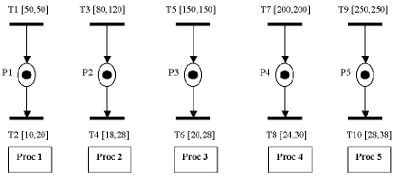
Figure 6: $TPN$ used in the experiments.

Table 3: Results of experiments performed on $TPN$.

Examples	Tools	TINA	ROMEO	ORIS	ITPNAnalyzer
		DBM	DBM	DBM	DBM	Tdis
	Classes	2	2	2	2	2
Proc 1	Edges	2	2	$NA$	2	2
	Times (ms)	0	$NA$	0	0	0
	Classes	186	186	188	186	186
Proc 1 2	Edges	262	262	$NA$	262	262
	Times (ms)	0	$NA$	16	0	0
	Classes	958	958	1.038	958	958
Proc 1 2 3	Edges	1506	1506	$NA$	1506	1506
	Times (ms)	16	$NA$	391	5	30
	Classes	5.219	5.219	6.029	5.219	5.219
Proc 1 2 3 4	Edges	8.580	8.580	$NA$	8.580	8.580
	Times (ms)	140	$NA$	2.719	38	80
	Classes	42.909	42.909	52.452	42.909	42.909
Proc 1 2 3 4 5	Edges	73.842	73.842	$NA$	73.842	73.842
	Times (ms)	6.739	$NA$	30.000	670	1.310

The first tests that have been carried out intended to verify whether our $\mathit{TPN}$ graph construction produce the same graphs as when using other tools. For this effect, we have considered the combination of the $\mathit{TPNs}$ shown in $\mathit{Fig.6}$. First, we started by testing the net Proc1, then we composed Proc1 with Proc2,  and so on. The results of these experiments are reported in $\mathit{Table}$ $\mathit{3}$. The latter shows that all graphs are identical except for ORIS which extends the expression of a class to the parameter $NEW$. In other respects, as it was expected, the times needed to compute the DBM state class graphs are faster than when computing the time distance based graphs.

The second series of tests that have been performed aimed at comparing the construction of the graph $\widetilde{GRc}$ with other graph construction approaches. For this effect, we considered the $ITPN$ model shown in Fig.7 while varying the intervals of transitions t${}_{2},$ and t₃. The results of these tests are reported in $\mathit{Table}$ $\mathit{4}$. This $ITPN,$ presented previously in [5], describes three independent tasks that are in conflict for a common resource (e.g a processor), and given respectively by the following pairs of transitions: Task₁=$(t_{1},t_{4})$, Task₂=$(t_{2},t_{5})$ and Task₃=$(t_{3},t_{6})$. Task 1 has a higher priority than the two other tasks, and Task 2 has priority on the Task 3. The priorities are characterized by using inhibitors arcs that connect the place $p_{1}$ to the transitions $t_{5}$ and $t_{6};$ and the place $p_{2}$ to the transition $t_{6}.$

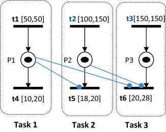
Figure 7: An ITPN example modeling three conflicting tasks.

For this purpose, different approaches have been tested: The exact graph construction defined in [10] and its DBM overapproximation defined in [9] which are both implemented in $\mathit{ROMEO}$; the DBM overapproximation defined in [16] and the time distance based approximation defined in this paper which are both implemented in $\mathit{ITPN\ Analyzer}$; the DBM overapproximation defined in [5] and implemented in $\mathit{ORIS}$; and finally, the K-grid based approximation defined in [8] and implemented in $TINA$. Notice that for the latter construction, we have considered the highest grid to approximate the polyhedra. In this case, this approach succeeds to compute the exact graph in almost all cases, but nevertheless with the highest cost.

Table 4: Results of experiments performed on $\mathit{ITPN}$.

	TOOLS	TINA	ROMEO		ITPN Analyser		ORIS
Examples	Methods	K-grid	Exact	DBM	$\widetilde{GR}(DBM)$	$\widetilde{GRc}(TDis)$	DBM
t2 [100,150]	Classes	4.489	4.489	5.431	5.378	4.483	5.538
t3 [160,160]	Edges	6.360	6.360	7.608	7.530	6.345	NA
	Times(ms)	1632	NA	NA	60	80	1578
t2 [80,120]	Classes	27.901	NF	47.777	39.648	27.889	40.414
t3 [145,145]	Edges	40.073	NF	67.754	56.238	40.163	NA
	Times(ms)	5.086	NA	NA	300	530	5.360
t2 [80,120]	Classes	29.976	NF	47.888	42.247	29.964	42.733
t3 [165,165]	Edges	42.844	NF	67.546,	59.635	42.832	NA
	Times(ms)	5.522	NA	NA	220	580	5.188
t2 [100,150]	Classes	16.913	16.913	21.033	20.802	16.901	21.116
t3 [145,145]	Edges	23.583	23.583	28.989	28.635	23.571	NA
	Times(ms)	2.870	NA	NA	170	230	5157
t2 [100,150]	Classes	320	320	403	394	319	429
t3 [150,150]	Edges	460	460	575	562	459	NA
	Times(ms)	110	NA	NA	4	10	156
t2 [100,150]	Classes	4.142	4.142	5.034	4.982	4.136	5140
t3 [140,140]	Edges	5.889	5.889	7.095	7.014	5.883	NA
	Times(ms)	1502	NA	NA	20	80	1.765
t3 [80,120]	Classes	28 392	NF	47.622	40.842	28.920	41.368
t5 [155,155]	edges	41.452	NF	67.309	57.766	41.440	NA
	Times (ms)	15703	NA	NA	280	640	9.062
t2 [80,120]	Classes	7.018	7.018	12.379	10.004	7.012	10.400
t3 [140,140]	Edges	10.242	10.242	17.829	14.406	10.236	NA
	Times(ms)	2834	NA	NA	50	140	3.516
t2 [100,150]	Classes	11.351	11.351	16.354	15.178	11.339	15.318
t3 [135,135]	Edges	15.649	15.649	22.230	20.486	15.639	NA
	Times(ms)	4907	NA	NA	90	230	4765
t2 [100,150]	Classes	17.612	17.612	21.857	21.626	17.600	21.942
t3 [155,155]	Edges	24.522	24.522	30.065	29.711	24.520	NA
	Times(ms)	7951	NA	NA	130	230	5594

As we notice, the graphs computed by the considered DBM overapproximations are not identical. As concerns $ORIS,$ the reason is given above.However for ROMEO, we have shown in [16] that the $DBM$ approximation defined in [9] is not truly implemented. In actual fact, in ROMEO the normalization of the DBM system is performed after removing the polyhedral inequalities, whereas it must be done before, thus yielding a loss of precision in the resulted graphs. It is noteworthy that among these DBM overapproximations, the approach defined in [16] and implemented in [22] is the one that computes the tightest graphs with the fastest times. Concerning the time distance based approximation defined in this paper, the results show that the obtained graphs are of the sime size relatively to the exact ones, even smaller. Moreover, the times needed for their computation are 10 even 20 times faster than those of TINA, and slightly more comparing to ROMEO.

It should be noticed that although the $\widetilde{GRc}$ is almost equal to $GR$, it still remains an overapproximation of it. In actual fact, many classes that stand unequal in $GR$ despite they are bisimilar, become equivalent when they are approximated in $\widetilde{GRc},$ thus compacting its size comparatively to the graph $GR$.

Table 5: WCRT and BCRT estimation of Task 3.

Examples	Methods	$\widetilde{GR}(DBM)$	$\widetilde{GRc}(Tdis)$	Exact
t2 [100,150]	WCRT	126	88	88
t3 [160,160]	BCRT	20	20	20
t2 [100,150]	WCRT	126	88	88
t3 [150,150]	BCRT	30	30	30
t2 [80,120]	WCRT	198	128	128
t3 [130,130]	BCRT	20	20	20
t2 [100,150]	WCRT	126	88	88
t3 [135,135]	BCRT	20	20	20
t2 [100,150]	WCRT	126	88	88
t3 [155,155]	BCRT	20	20	20
t2 [80,120]	WCRT	208	128	128
t3 [140,140]	BCRT	20	20	20

The final tests, results of which are given in $\mathit{Tab}$ $\mathit{5,}$ report the obtained BCRT and WCRT of Task 3, while assuming different graph constructions. As we can see, the computed values of the BCRT are the same for all the nets whatever the graph construction we consider. On the other hand, the WCRT is differently estimated following the approach we use. When considering the graph $\widetilde{GR}$, the approximated values are too coarse as it is the case in the tests 3 and 6. However, the $\widetilde{GRc}$ preserves the exact value of the WCRT for all the tested nets. These results show how tight this approximation is, because the additional sequences that are distorting the estimation of the WCRT in the graph $\widetilde{GR}$ are completely removed in the $\widetilde{GRc}$.

5 Conclusion

We have proposed in this paper a novel approach to compute an overapproximation of the state space of real time preemptive systems modeled using the $ITPN$ model. For this effect, we have defined the time distance system that encodes the quantitative properties of each class of states reachable in the exact graph. Then we have provided efficient algorithms to overapproximate its coefficients and to compute the DBM overapproximation of a class. We proved that this construction is more precise than other classical DBM overapproximation defined in the literature [16] [9][5], and showed how it is appropriate to restore the quantitative properties of the model. Simulation results comparing the performances of our graph construction with other techniques were reported.

6 APPENDIX A : Proof of Theorem 1

We have to determine the following clauses:

1. $\left\rceil D^{0}\right\lceil=\left\rceil\widetilde{D^{0}}\right\lceil=\left\rceil\widetilde{D_{c}^{0}}\right\lceil$ and $\left\rceil DS^{0}\right\lceil=\left\rceil\widetilde{DS^{0}}\right\lceil$

2. Let be $S=(t_{f}^{1},..,t_{f}^{n});$ if $(M^{0},D^{0})\overset{t_{f}^{1}}{\longmapsto}..\overset{t_{f}^{n-1}}{\longmapsto}E^{n-1}=(M^{n-1},D^{n-1})$ ,
   $(M^{0},Ne^{0},Ni^{0},Na^{0},\widetilde{DS^{0}},\widetilde{D_{c}^{0}})\overset{t_{f}^{1}}{\leadsto}..\overset{t_{f}^{n-1}}{\leadsto}\widetilde{E_{c}^{n-1}}=(M^{n-1},Ne^{n-1},Ni^{n-1},Na^{n-1},\widetilde{DS^{n-1}},\widetilde{D_{c}^{n-1}})$, and $(M^{0},\widetilde{D^{0}})\overset{t_{f}^{1}}{\rightsquigarrow}..\overset{t_{f}^{n-1}}{\rightsquigarrow}\widetilde{E^{n-1}}=(M^{n-1},\widetilde{D^{n-1}})$ such that $\left\rceil D^{n-1}\right\lceil\subseteq\left\rceil\widetilde{D_{c}^{n-1}}\right\lceil\subseteq\left\rceil\widetilde{D^{n-1}}\right\lceil$ and $\left\rceil DS^{n-1}\right\lceil\subseteq\left\rceil\widetilde{DS^{n-1}}\right\lceil$ ; we have : if $E^{n-1}\overset{t_{f}^{n}}{\longmapsto}E^{n}=(M^{n},D^{n}),$ then

   • $\widetilde{E^{n-1}}\overset{t_{f}^{n}}{\rightsquigarrow}\widetilde{E^{n}}=(M^{n},\widetilde{D^{n}}),$

   • $\widetilde{E_{c}^{n-1}}$$\overset{t_{f}^{n}}{\leadsto}\widetilde{E_{c}^{n}}=(M^{n},Ne^{n},Ni^{n},Na^{n},\widetilde{DS^{n}},\widetilde{D_{c}^{n}})$

   • and we have $\left\rceil D^{n}\right\lceil\subseteq\left\rceil\widetilde{D_{c}^{n}}\right\lceil\subseteq\left\rceil\widetilde{D^{n}}\right\lceil$ and $\left\rceil DS^{n}\right\lceil\subseteq\left\rceil\widetilde{DS^{n}}\right\lceil$

The clause $(1)$ holds since the system $D$⁰ is in $DBM$ ; we have by definition :  $D^{0}=\widetilde{D_{c}^{0}}=\widetilde{D^{0}}$ and $DS^{0}=\widetilde{DS^{0}}.$ Let us prove now the clause $(2).$ Let us assume $D^{n-1}=\widehat{{D^{n-1}}}\wedge$$\overrightarrow{{D^{n-1}}}.$ The system $\overrightarrow{D^{n-1}}$ denotes the tightest DBM system extracted from the system ${D}^{{n}}$, and is given by all its normalized DBM inequalities, as follows:

$\left\{\begin{tabular}[]{l}$B_{1}:\forall t_{{}_{1}}\neq t_{{}_{2}}\in Te(M^{n-1}),\quad\underline{t_{{}_{2}}}-\underline{t_{{}_{1}}}\leq\overrightarrow{D^{n-1}}[t_{{}_{1}},t_{{}_{2}}]\quad$\\ $B_{2}:\forall t\in Te(M^{n-1}),\quad-\overrightarrow{D^{n-1}}[t,\bullet]\leq\underline{t}\leq\overrightarrow{D^{n-1}}[\bullet,t]\quad$\end{tabular}\right.$

According to the hypotheses of the Clause 2, as we have $\left\rceil D^{n-1}\right\lceil\subseteq\left\rceil\overrightarrow{D^{n-1}}\right\lceil\subseteq\left\rceil\widetilde{D_{c}^{n-1}}\right\lceil\subseteq\left\rceil\widetilde{D^{n-1}}\right\lceil$ then the following properties hold:

$\left\{\begin{tabular}[]{l}$P_{1}:\forall t_{{}_{1}}\neq t_{{}_{2}}\in Te(M^{n-1}),\quad\overrightarrow{D^{n-1}}[t_{{}_{1}},t_{{}_{2}}]\leq\widetilde{D_{c}^{n-1}}[t_{{}_{1}},t_{{}_{2}}]\leq\widetilde{D^{n-1}}[t_{{}_{1}},t_{{}_{2}}].\quad$\\ $P_{2}:\forall t\in Te(M^{n-1}),\quad\overrightarrow{D^{n-1}}[t,\bullet]\leq\widetilde{D_{c}^{n-1}}[t,\bullet]\leq\widetilde{D^{n-1}}[t,\bullet].\quad$\\ $P_{3}:\forall t\in Te(M^{n-1}),\quad\overrightarrow{D^{n-1}}[\bullet,t]\leq\widetilde{D_{c}^{n-1}}[\bullet,t]\leq\widetilde{D^{n-1}}[\bullet,t].\quad$\end{tabular}\right.$

Let us consider now the firing of the transition $t_{f}^{n}$ from $E^{n-1}$ to reach the class $E^{n}$$=(M^{n},D^{n})$. So that $t_{f}^{n}$ can be fired from $E^{n-1}$ we must have: $t_{f}^{n}\in Ta(M^{n-1})$ and$\quad B_{3}:$ $\forall t\in Ta(M^{n-1})\quad 0\leq$$t_{f}^{n}$$\leq$$t$.  Therefore, if $t_{f}^{n}$ is firable from $E^{n-1},$ then the system $\left\rceil D^{n-1}\wedge B_{3}\right\lceil\neq\emptyset;$ hence we have $\forall t\in Ta(M^{n-1}),$ $\overrightarrow{D^{n-1}}[t_{f},t]\geq 0$. By using the property $(P_{1})$, we deduce that $\forall t\in Ta(M^{n-1})$ we have $\widetilde{D^{n-1}}[t_{f}^{n},t]\geq 0$ and $\widetilde{D_{c}^{n-1}}[t_{f}^{n},t]\geq 0$. Hence $\widetilde{\beta^{n}}[t_{f}^{n}]\ \geq 0$ and $\widetilde{\beta_{c}^{n}}[t_{f}^{n}]\ \geq 0.$ Consequently, $t_{f}^{n}$ is also firable from the classes $\widetilde{{\small E}_{{\small c}}^{{\small n-1}}}$ and $\widetilde{{\small E}^{{\small n-1}}}.$ It remains to prove that $\left\rceil DS^{n}\right\lceil\subseteq\left\rceil\widetilde{DS^{n}}\right\lceil$ and $\left\rceil\overrightarrow{D^{n}}\right\lceil\subseteq\left\rceil\widetilde{D_{c}^{n}}\right\lceil\subseteq\left\rceil\widetilde{D^{n}}\right\lceil$.  This requires first to prove that the system $\widetilde{DS^{n}}\$is always an overapproximation of the system ${\small DS^{n},}$ namely that each coefficient of $\widetilde{DS^{n}}$ is equal or greater than its related in ${\small DS^{n-1}}$. For this effect, let us assume the systems $\widetilde{{\small DS^{n-1}}}$  and ${\small DS^{n-1}}$ associated respectively with the class $\widetilde{E_{c}^{n-1}}$ and $E^{n-1}$ given as follows:

$\left\{\begin{tabular}[]{l}$C_{1}:{\Huge\wedge}_{\forall i\in Point^{n-1}}-\widetilde{DS^{n-1}}[n-1,i]\leq\underline{t_{f}^{{}_{i+1}}}+..+\underline{t_{f}^{n-1}}\leq\widetilde{DS^{n-1}}[i,n-1]$\newline \\ $C_{2}:${\Huge$\wedge$}${}_{\forall t\in Te(M^{n-1})}{\Huge\wedge}_{\forall i\in Point^{n-1}\cup\{n-1\}}-\widetilde{DS^{n-1}}[t,i]\leq\underline{t_{f}^{{}_{i+1}}}+..+\underline{t_{f}^{n-1}}+\underline{t}\leq\widetilde{DS^{n-1}}[i,t]$\end{tabular}\newline \right.$

$\left\{\begin{tabular}[]{l}$C_{3}:{\Huge\wedge}_{\forall i\in Point^{n-1}}-DS^{n-1}[n-1,i]\leq\underline{t_{f}^{{}_{i+1}}}+..+\underline{t_{f}^{n-1}}\leq DS^{n-1}[i,n-1]$\newline \\ $C_{4}:{\Huge\wedge}_{\forall t\in Te(M^{n-1})}{\Huge\wedge}_{\forall i\in Point^{n-1}\cup\{n-1\}}-DS^{n-1}[t,i]\leq\underline{t_{f}^{{}_{i+1}}}+..+\underline{t_{f}^{n-1}}+\underline{t}\leq DS^{n-1}[i,t]$\end{tabular}\newline \right.$

According to the hypotheses of the Clause 2, as we have $\left\rceil DS^{n-1}\right\lceil\subseteq\left\rceil\widetilde{Ds^{n-1}}\right\lceil$ then the following properties hold:

$\left\{\begin{tabular}[]{l}$P_{4}:\forall i\in point^{n-1},DS^{n-1}[n-1,i]\leq\widetilde{DS^{n-1}}[n-1,i]\quad$\\ $P_{5}:\forall i\in point^{n-1},DS^{n-1}[i,n-1]\leq\widetilde{DS^{n-1}}[i,n-1]$\\ $P_{6}:\forall i\in point^{n-1}\cup\{n-1\},\forall t\in Te(M^{n-1}),\quad DS^{n-1}[t,i]\leq\widetilde{DS^{n-1}}[t,i]$\\ $P_{7}:\forall i\in point^{n-1}\cup\{n-1\},\forall t\in Te(M^{n-1}),\quad DS^{n-1}[i,t]\leq\widetilde{DS^{n-1}}[i,t]$\end{tabular}\right.$

Let assume now the systems $\widetilde{{\small DS^{n}}}$  and ${\small DS^{n}}$ associated respectively with the classes $\widetilde{E_{c}^{n}}$ and $E^{n}$ obtained after firing the transition ${\small t}_{{\small f}}^{{\small n}}$:

$\left\{\begin{tabular}[]{l}$F_{1}:{\Huge\wedge}_{\forall i\in Point^{n}}-\widetilde{DS^{n}}[n,i]\leq\underline{t_{f}^{{}_{i+1}}}+..+\underline{t_{f}^{n}}\leq\widetilde{DS^{n}}[i,n]$\newline \\ $F_{2}:{\Huge\wedge}_{\forall i\in Point^{n}\cup\{n\}}${\Huge$\wedge$}${}_{\forall t^{\prime}\in Te(M^{n})}-\widetilde{DS^{n}}[t^{\prime},i]\leq\underline{t_{f}^{{}_{i+1}}}+..+\underline{t_{f}^{n}}+\underline{t}^{\prime}\leq\widetilde{DS^{n}}[i,t^{\prime}]$\end{tabular}\newline \right.$

$\left\{\begin{tabular}[]{l}$F_{3}:{\Huge\wedge}_{\forall i\in Point^{n}}-DS^{n}[n-1,i]\leq\underline{t_{f}^{{}_{i+1}}}+..+\underline{t_{f}^{n}}\leq DS^{n}[i,n]$\newline \\ $F_{4}:{\Huge\wedge}_{\forall i\in Point^{n}\cup\{n\}}${\Huge$\wedge$}${}_{\forall t^{\prime}\in Te(M^{n})}-DS^{n}[t^{\prime},i]\leq\underline{t_{f}^{{}_{i+1}}}+..+\underline{t_{f}^{n}}+\underline{t}^{\prime}\leq DS^{n}[i,t^{\prime}]$\end{tabular}\newline \right.$

We need to prove that :

$\left\{\begin{tabular}[]{l}$P_{4}^{\prime}:\forall i\in point^{n},DS^{n}[n,i]\leq\widetilde{DS^{n}}[n,i]\quad$\\ $P_{5}^{\prime}:\forall i\in point^{n},DS^{n}[i,n]\leq\widetilde{DS^{n}}[i,n]$\\ $P_{6}^{\prime}:\forall i\in point^{n}\cup\{n\},\forall t^{\prime}\in Te(M^{n}),\quad DS^{n}[t^{\prime},i]\leq\widetilde{DS^{n}}[t^{\prime},i]$\\ $P_{7}^{\prime}:\forall i\in point^{n}\cup\{n\},\forall t^{\prime}\in Te(M^{n}),\quad DS^{n}[i,t^{\prime}]\leq\widetilde{DS^{n}}[i,t^{\prime}]$\end{tabular}\right.$

First of all, we have: $\forall i$ $\in\left[Ne^{n}\right]-\{n\}$, then $i$ $\in\left[Ne^{n-1}\right]$, namely all persistent transitions reported at point $(n)$ keep their same enabling point as in the firing point $(n-1)$. Furthermore,$\forall i\in\left[Ni^{n}\right]-\{n\}$, then $i$ $\in\left[Ni^{n-1}\right].$ In other words, all persistent inhibited transitions reported at point $(n)$ enjoy the same inhibiting point as for the point $(n-1)$. Finally,$\forall i\in\left[Na^{n}\right]-\{n\}$, then $i$ $\in\left[Na^{n-1}\right],$ namely all persistent activated transitions reported at point $(n)$ enjoy the same activating point as for the point $(n-1)$. Therefore, we have: $\ {\small(P}_{{\small 8}}^{\prime}{\small):}$$\forall i$ $\in Point^{n}-\{n\}$, then $i$ $\in Point^{n-1}.$

As described in Definitions 7, the computation of the system $DS^{n}$ is performed by replacing each variable $t$ associated with a persistent activated transition $t\in Ta(M^{n-1})-\left\{t_{f}^{n}\right\}$ by $\underline{t^{{}^{\prime}}}+\underline{t_{f}^{n}}.$ However, each variable $\underline{t}$ connected to a persistent inhibited transition is replaced with $\underline{t^{{}^{\prime}}}.$  The coefficients of $DS^{n}$ are determined by intersection of the inequalities of predecessor systems in the sequence, namely $D_{a}^{n-1}$ and $DS^{n-1}$.

• Let us determine first the proprerties $P_{4}^{\prime}$ and $P_{5}^{\prime}.$ To this end, we restrain our constraint manipulations by summing only the inequalities of $B_{3}:$$\forall t\in Ta(M^{n-1})$    $t_{f}^{n}$$\leq t$ with the right part of $C_{4}$, we obtain:
  $\forall t\in Ta(M^{n-1})\quad$$\underline{t_{f}^{{}_{i+1}}}+..+\underline{t_{f}^{n-1}}+$$t_{f}^{n}$$+\underline{t}\leq DS^{n-1}[i,t]+\underline{t}.$
  Let us remove the variable $\underline{t}$ from both parts of the previous inequalities:
  $\underline{t_{f}^{{}_{i+1}}}+..+\underline{t_{f}^{n-1}}+$$t_{f}^{n}$$\leq\underset{\forall t\in Ta(M^{n-1})}{MIN}DS^{n-1}[i,t]$
  On the other side, let us consider the left part of the constraint $C_{4}$ while assuming $\underline{t}$ =$t_{f}^{n}$, we obtain: $-DS^{n-1}[t_{f}^{n},i]\leq\underline{t_{f}^{{}_{i+1}}}+..+\underline{t_{f}^{n}}$
  Hence, we determine that : 
   $-DS^{n-1}[t_{f}^{n},i]\leq-DS^{n}[n,i]\leq\underline{t_{f}^{{}_{i+1}}}+..+\underline{t_{f}^{n}}\leq DS^{n}[i,n]\leq\underset{\forall t\in Ta(M^{n-1})}{MIN}DS^{n-1}[i,t]$.
  Then by using the properties ${\small P}_{{\small 4}}{\small..P}_{{\small 6}}$, we deduce :
  $-\widetilde{DS^{n-1}}[t_{f}^{n},i]\leq-DS^{n}[n,i]\leq\underline{t_{f}^{{}_{i+1}}}+..+\underline{t_{f}^{n}}\leq DS^{n}[i,n]\leq$$\lambda^{n-1}[i]$.
  Then according to Proposition 1, we prove ${\small P}_{{\small 4}}^{\prime}$ and ${\small P}_{{\small 5}}^{\prime}$:
  $-\widetilde{DS^{n}}[n,i]\leq-DS^{n}[n,i]\leq\underline{t_{f}^{{}_{i+1}}}+..+\underline{t_{f}^{n}}\leq DS^{n}[i,n]\leq\widetilde{DS^{n}}[i,n]$.

To determine now the proprerties ${\small P}_{{\small 5}}^{\prime}$ and ${\small P}_{{\small 6}}^{\prime}$ we have to consider first the status of the transition $t^{\prime}$ at the firing point $(n)$.

• Case where $t^{\prime}$ is newly enabled for $M^{n}:$ Therefore the variable $t^{\prime}$ is new in $DS^{n}$ and has not been obtained by renaming another variable of $DS^{n-1}$. So by intersection of the constraints of ${\small tmin(t}^{\prime}{\small)\leq\underline{t}^{\prime}\leq tmax(t}^{\prime}{\small)}$  and $F_{3},$ we determine:
  $-DS_{n}[n,i]+tmin(t^{\prime})\leq\underline{t_{f}^{{}_{i+1}}}+..+\underline{t_{f}^{n}}+\underline{t}^{\prime}\leq DS^{n}[i,n]+$${\small tmax(t}^{\prime}{\small).}$
  Then, according to Proposition 1 and by using the properties ${\small P}_{{\small 4}}{\small..P}_{{\small 6}}$, we prove ${\small P}_{{\small 5}}^{\prime}$ and ${\small P}_{{\small 6}}^{\prime}$:$-\widetilde{DS^{n}}[t^{\prime},n]\leq-DS^{n}[t^{\prime},n]\leq\underline{t_{f}^{{}_{i+1}}}+..+\underline{t_{f}^{n}}+\underline{t}^{\prime}\leq DS^{n}[i,t^{\prime}]\leq\widetilde{DS^{n}}[i,t^{\prime}]$.

• Case where $t^{\prime}$ is persistent for $M^{n}:$ Therefore, ${\small r=}$$Ne^{n}(t)=Ne^{n-1}(t)\neq n$ and the variable $t^{\prime}$ has been obtained by renaming another variable of $D^{n-1}$. Let us assume ${\small s=}$$Ni^{n-1}(t)$ and $p=Na^{n-1}(t).$

  Case 1: $\forall i\in Point^{n}-\left\{n\right\}$ : We should consider the status of the original variable $t$ in $E^{n-1}.$ 

  • If $t$ is activated for $M^{n-1}$, then the variable $t$ was renamed by $\underline{t^{{}^{\prime}}}$ in $DS^{n}$ and we have $t=$ $\underline{t^{{}^{\prime}}}+\underline{t_{f}^{n}}.$
    Let us consider the constraint $F_{3}$ while assuming the points ${\small i,}$ $p$ and $s;$ we obtain :
    $(G_{1}):$ $-DS^{n}[n,i]\leq\underline{t_{f}^{{}_{i+1}}}+..+\underline{t_{f}^{n}}\leq DS^{n}[i,n].$
    $(G_{2}):$ $-DS^{n}[n,p]\leq\underline{t_{f}^{{}_{p+1}}}+..+\underline{t_{f}^{n}}\leq DS^{n}[p,n].$
    $(G_{3}):$ $-DS^{n}[n,s]\leq\underline{t_{f}^{{}_{s+1}}}+..+\underline{t_{f}^{n}}\leq DS^{n}[s,n].$
    

    Now let us consider the systems $DS^{\mathit{s}}$ and $DS^{\mathit{i}}$ computed respectively at points ${\small s}$ and ${\small i}$, where we deal with the constraint of type ${\small C}_{{\small 4}}$:
    If ($i\leq s$) this means that $t$ was inhibited at point $(s)$ after having already reached the point $(i)$. Therefore, we have: $i\in Point^{s}$ and $-DS^{\mathit{s}}[t,i]\leq\underline{t_{f}^{{}_{i+1}}}+..+\underline{t_{f}^{s}}+\underline{t}{{}^{\circ}}\leq DS^{\mathit{s}}[i,t];$ where $t{{}^{\circ}}$ is the original name of the variable related to transition $t$ in $E^{s}$. Hence, as ${\small t}$ is inhibited in the point interval ${\small[s,p]}$ we replace $t{{}^{\circ}}$ in the previous constraint with $\underline{t_{f}^{{}_{p+1}}}+..+\underline{t_{f}^{n}}+\underline{t}^{\prime}$ we obtain:
    $(G_{4}):-DS^{\mathit{s}}[t,i]\leq\underline{t_{f}^{{}_{i+1}}}+..+\underline{t_{f}^{s}}+\underline{t_{f}^{{}_{p+1}}}+..+\underline{t_{f}^{n}}+\underline{t}^{\prime}\leq DS^{\mathit{s}}[i,t];$

    Otherwise, if ($i>s$) this means that $t$ was inhibited at point $(s)$ before reaching the point $(i)$. Therefore, we have: $i\notin point$^s but $s\in point$ⁱ and $-DS^{\mathit{i}}[t,i]\leq\underline{t}^{\ast}\leq DS^{\mathit{i}}[i,t];$ where $t^{\ast}$ is the original name of the variable related to transition $t$ in $E^{i}$. Hence, as ${\small t}$ is inhibited in the point interval ${\small[i,p]}$ we replace $t$^∗ in the previous constraint with $\underline{t_{f}^{{}_{p+1}}}+..+\underline{t_{f}^{n}}+\underline{t}^{\prime}$ we obtain:
    $(G_{5}):-DS^{\mathit{i}}[t,i]\leq\underline{t_{f}^{{}_{p+1}}}+..+\underline{t_{f}^{n}}+\underline{t}^{\prime}\leq DS^{\mathit{i}}[i,t];$

    Note recalling that all the variables $t$$,\underline{t^{\prime}},\underline{t{{}^{\circ}}}$ and $t^{\ast}$ relate to the same occurence of the transition ${\small t}$ since ${\small t}$ remains persistently enabled in the firing sequence till the point $(n)$.

    Case ($i\leq s$): By summing ${\small G}_{{\small 4}}$ and ${\small G}_{{\small 3}}$ and then by intersection with ${\small G}_{{\small 2}}$, we obtain:

    $(H_{1}):-DS^{\mathit{s}}[t,i]-DS^{\mathit{n}}[p,n]-DS^{\mathit{n}}[n,s]\leq-DS^{\mathit{n}}[t,i]\leq\underline{t_{f}^{{}_{i+1}}}+..+\underline{t_{f}^{n}}+\underline{t}^{\prime}\leq DS^{\mathit{n}}[i,t]\leq DS^{\mathit{s}}[i,t]+DS^{\mathit{n}}[n,p]+DS^{\mathit{n}}[s,n];$

    Case ($s<i$): By summing ${\small G}_{{\small 5}}$ and ${\small G}_{{\small 1}}$ and then by intersection with ${\small G}_{{\small 2}}$, we obtain:

    $(H_{2}):-DS^{\mathit{i}}[t,i]-DS^{\mathit{n}}[p,n]-DS^{\mathit{n}}[n,i]\leq-DS^{\mathit{n}}[t,i]\leq\underline{t_{f}^{{}_{i+1}}}+..+\underline{t_{f}^{n}}+\underline{t}^{\prime}\leq DS^{\mathit{n}}[i,t]\leq DS^{\mathit{i}}[i,t]+DS^{\mathit{n}}[n,p]+DS^{\mathit{n}}[i,n];$
    On the other hand, let us consider now the constraint $C_{4},$ we have:
    $-DS^{n-1}[t,i]\leq\underline{t_{f}^{{}_{i+1}}}+..+\underline{t_{f}^{n-1}}+\underline{t}\leq DS^{n-1}[i,t]$
    We put $\underline{t}$ $=$ $\underline{t^{{}^{\prime}}}+\underline{t_{f}^{n}},$ we obtain $:$ $-DS^{n-1}[t,i]\leq\underline{t_{f}^{{}_{i+1}}}+..+\underline{t_{f}^{n}}+\underline{t}^{\prime}\leq DS^{n-1}[i,t]$
    $(H_{3}):$ $-DS^{n-1}[t,i]\leq-DS^{n}[t,i]\leq\underline{t_{f}^{{}_{i+1}}}+..+\underline{t_{f}^{n}}+\underline{t}^{\prime}\leq DS^{n}[i,t]\leq DS^{n-1}[i,t]$
    In other respects, by intersection of ${\small B}_{{\small 3}}$ and ${\small C}_{{\small 4}}$, and then summing with ${\small G}_{{\small 1}}$, we obtain:
    $(H_{4}):-DS^{\mathit{n}}[n,i]-MIN(0,DS^{\mathit{n-1}}[t,n-1]+\lambda^{\mathit{n-1}}[n-1])\leq-DS^{\mathit{n}}[t,i]\leq\underline{t_{f}^{{}_{i+1}}}+..+\underline{t_{f}^{n}}+\underline{t}^{\prime}\leq DS^{\mathit{n}}[i,t]\leq DS^{\mathit{n}}[i,n]+DS^{\mathit{n-1}}[n-1,t]+DS^{\mathit{n-1}}[t_{f}^{n},n-1];$
    Finally, from ${\small H}_{{\small 1}}{\small,H}_{{\small 2}}{\small,H}_{{\small 3}}$ and ${\small H}_{{\small 4}}$, by using previous established properties and according to proposition 1, we determine ${\small P}_{{\small 6}}^{\prime}$ and ${\small P}_{{\small 7}}^{\prime}$ :
    $-DS^{\mathit{n}}[t,i]\leq-\widetilde{DS^{\mathit{n}}}[t,i]\leq\underline{t_{f}^{{}_{i+1}}}+..+\underline{t_{f}^{n}}+\underline{t}^{\prime}\leq DS^{\mathit{n}}[i,t]\leq\widetilde{DS^{\mathit{n}}}[i,t].\vskip 6.0pt plus 2.0pt minus 2.0pt$

  • If $t$ is inhibited for $M^{n-1}$, then $t$ was renamed by $\underline{t^{{}^{\prime}}}$ in $DS^{n}$ and we have $t=$ $\underline{t^{{}^{\prime}}}.$
    Let us consider first the constraint $C_{4},$ we have:
    $-DS^{n-1}[t,i]\leq\underline{t_{f}^{{}_{i+1}}}+..+\underline{t_{f}^{n-1}}+\underline{t}\leq DS^{n-1}[i,t]$
    We put $\underline{t}$ $=$ $\underline{t^{{}^{\prime}}},$ we obtain ${\small(G}_{{\small 1}}^{\prime}{\small):}$ $-DS^{n-1}[t,i]\leq\underline{t_{f}^{{}_{i+1}}}+..+\underline{t_{f}^{n-1}}+\underline{t}^{\prime}\leq DS^{n-1}[i,t].$
    In other respects, by intersection of ${\small B}_{{\small 3}}$ with ${\small C}_{{\small 4}}$, and then summing with ${\small G}_{{\small 1}}^{\prime}$, we obtain:
    $(H_{1}^{\prime}):-DS^{\mathit{n-1}}[t,i]-DS^{\mathit{n-1}}[t_{f}^{n},n-1]\leq-DS^{\mathit{n}}[t,i]\leq\underline{t_{f}^{{}_{i+1}}}+..+\underline{t_{f}^{n}}+\underline{t}^{\prime}\leq DS^{\mathit{n}}[i,t]\leq\lambda^{\mathit{n-1}}[n-1]+DS^{\mathit{n-1}}[i,t];$

    Let us consider the constraint $F_{3}$ while assuming the points $s$ and ${\small i}$, we obtain :
    $(G_{2}^{\prime}):$ $-DS^{n}[n,s]\leq\underline{t_{f}^{{}_{s+1}}}+..+\underline{t_{f}^{n}}\leq DS^{n}[s,n].$
    $(G_{3}^{\prime}):$ $-DS^{n}[n,i]\leq\underline{t_{f}^{{}_{i+1}}}+..+\underline{t_{f}^{n}}\leq DS^{n}[i,n].$
    

    Now let us consider the systems $DS^{\mathit{s}}$ and $DS^{\mathit{i}}$ computed respectively at point ${\small s}$ and ${\small i}$, where we deal with the constraint of type ${\small C}_{{\small 4}}$:
    If ($i\leq s$) this means that $t$ was inhibited at point $(s)$ after having already reached the point $(i)$ and still remains persistently inhibited till point ${\small(n)}$. Therefore, we have: $i\in Point^{s}$ and $-DS^{\mathit{s}}[t,i]\leq\underline{t_{f}^{{}_{i+1}}}+..+\underline{t_{f}^{s}}+\underline{t}{{}^{\circ}}\leq DS^{\mathit{s}}[i,t];$ where $t{{}^{\circ}}$ is the original name of the variable related to transition $t$ in $E^{s}$. Hence, as ${\small t}$ is inhibited in the point interval ${\small[s,n]}$ we replace $t{{}^{\circ}}$ in the previous constraint with $\underline{t}^{\prime}$ we obtain:
    $(G_{4}^{\prime}):-DS^{\mathit{s}}[t,i]\leq\underline{t_{f}^{{}_{i+1}}}+..+\underline{t_{f}^{s}}++\underline{t}^{\prime}\leq DS^{\mathit{s}}[i,t];$

    Otherwise, if ($i>s$) this means that $t$ was inhibited at point $(s)$ before reaching the point $(i)$ and still remains persistently inhibited till point ${\small n}$. Therefore, we have: $i\notin point$^s but $s\in point$ⁱ and $-DS^{\mathit{i}}[t,i]\leq\underline{t}^{\ast}\leq DS^{\mathit{i}}[i,t];$ where $t^{\ast}$ is the original name of the variable related to transition $t$ in $E^{i}$. Hence, as ${\small t}$ is inhibited in the point interval ${\small[i,n]}$ we replace $t$^∗ in the previous constraint with $\underline{t}^{\prime}$ we obtain: $(G_{5}^{\prime}):-DS^{\mathit{i}}[t,i]\leq\underline{t}^{\prime}\leq DS^{\mathit{i}}[i,t];$

    Case ($i\leq s$): By summing ${\small G}_{{\small 4}}^{\prime}$ and ${\small G}_{{\small 2}}^{\prime}$ we obtain:

    $(H_{2}^{\prime}):-DS^{\mathit{s}}[t,i]-DS^{\mathit{n}}[n,s]\leq-DS^{\mathit{n}}[t,i]\leq\underline{t_{f}^{{}_{i+1}}}+..+\underline{t_{f}^{n}}+\underline{t}^{\prime}\leq DS^{\mathit{n}}[i,t]\leq DS^{\mathit{s}}[i,t]+DS^{\mathit{n}}[s,n];$

    Case ($s<i$): By summing ${\small G}_{{\small 5}}^{\prime}$ and ${\small G}_{{\small 3}}^{\prime}$, we obtain:

    $(H_{3}^{\prime}):-DS^{\mathit{i}}[t,i]-DS^{\mathit{n}}[n,i]\leq-DS^{\mathit{n}}[t,i]\leq\underline{t_{f}^{{}_{i+1}}}+..+\underline{t_{f}^{n}}+\underline{t}^{\prime}\leq DS^{\mathit{n}}[i,t]\leq DS^{\mathit{i}}[i,t]+DS^{\mathit{n}}[i,n];$
    Finally, from ${\small H}_{{\small 1}}^{\prime}{\small,H}_{{\small 2}}^{\prime}{\small,}$ and ${\small H}_{{\small 3}}^{\prime}$, by using previous established properties and according to proposition 1, we determine the properties :
    $-DS^{\mathit{n}}[t,i]\leq-\widetilde{DS^{\mathit{n}}}[t,i]\leq\underline{t_{f}^{{}_{i+1}}}+..+\underline{t_{f}^{n}}+\underline{t}^{\prime}\leq DS^{\mathit{n}}[i,t]\leq\widetilde{DS^{\mathit{n}}}[i,t].\vskip 6.0pt plus 2.0pt minus 2.0pt$

Case $i=n$:
 First of all, it should be noticed that we have by definition:
              $\widetilde{DS^{n}}[n,t]=\widetilde{D_{c}^{n}}[\bullet,t]$ and $\widetilde{DS^{n}}[t,n]=\widetilde{D_{c}^{n}[}t,\bullet].$ Moreover, we have : $DS^{n}[n,t]=\overrightarrow{D^{n}}[\bullet,t]$ and $DS^{n}[t,n]=\overrightarrow{D^{n}}[t,\bullet].$

• • If $t$ is activated for $M^{n-1}$:  From we properties ${\small P}_{{\small 1}}{\small..P}_{{\small 4}}$ we have : $\beta^{n-1}[t]\leq\widetilde{\beta_{c}^{n-1}}[t]\leq\widetilde{\beta^{n-1}}[t].$
    As already established in [16] and shown in Definition.5, when manipulating exclusively the DBM constraints of the normalized systems $\overrightarrow{{\small D^{n-1}}}$ or $\widetilde{{\small D_{c}^{n-1}}}$ or $\widetilde{{\small D^{n-1}}}$ we obtain:
    $(L_{1}):-\widetilde{\beta^{n-1}}[t]$ $\leq\underline{t}^{\prime}\leq$$\widetilde{{\small D^{n-1}}}$$[t_{f}^{n},t].\$
    $(L_{2}):-$${\small\beta^{n-1}{}}$$[t]$ $\leq\underline{t}^{\prime}\leq$$\overrightarrow{{\small D^{n-1}}}$$[t_{f}^{n},t].\$
    $(L_{3}):-$$\widetilde{{\small\beta_{c}^{n-1}}}$${}[t]$ $\leq\underline{t}^{\prime}\leq\widetilde{D_{c}^{n-1}}[t_{f}^{n},t].\$
    Let us consider now the constraints of $F_{3}$ and $F_{4}$ with $i=r$ :
    $-DS^{n}[t,r]\leq\underline{t_{f}^{{}_{r+1}}}+..+\underline{t_{f}^{n}}+\underline{t}^{\prime}\leq DS^{n}[r,t]$
    $-DS^{n}[n,r]\leq\underline{t_{f}^{{}_{r+1}}}+..+\underline{t_{f}^{n}}\leq DS^{n}[r,n]$
    By intersection of the previous constraints we obtain:
    $(L_{4}):-MIN(0,DS^{n}[t,r]+DS^{n}[r,n]\leq\underline{t}^{\prime}\leq DS^{n}[r,t]+DS^{n}[n,r]$
    From ${\small L}_{{\small 1}}{\small,..L}_{{\small 4}}$, Proposition 1 and Définition 5. Then by using already established properties, we deduce :
    ${\small-}$$\widetilde{D^{n}}[t,\bullet]\leq$ ${\small-}$$\widetilde{DS^{n}}[t,n]\leq-DS^{n}[t,n]\leq\underline{t}^{\prime}\leq DS^{n}[n,t]\leq$ $\widetilde{DS^{n}}[n,t]\leq$ $\widetilde{D^{n}}[\bullet,t]$.

  • If $t$ is inhibited for $M^{n-1}.$ As already established in [16] and shown in Definition.5,  when dealing exclusively with the DBM constraints of the normalized systems $\overrightarrow{{\small D^{n-1}}}$ or $\widetilde{{\small D_{c}^{n-1}}}$ or $\widetilde{{\small D^{n-1}}}$ we obtain:
    $(L_{1}^{\prime}):-MIN$$\left({\small\widetilde{D^{n-1}}[t,\bullet],}\text{ }{\small\widetilde{D^{n-1}}[t_{f}^{n},\bullet]+\ \widetilde{\beta^{n-1}}[t]}\right)$$\leq\underline{t}^{\prime}\leq MIN$$\left(\widetilde{{\small D^{n-1}}}{\small[\bullet,t],\ }\widetilde{{\small D^{n-1}}}{\small[t_{f}^{n},t]+\ }\widetilde{{\small\beta^{n-1}}}{\small[\bullet]}\right)$$.\$
    $(L_{2}^{\prime}):-MIN$$\left({\small\widetilde{DS^{n-1}}[t,n-1],}\text{ }{\small\widetilde{DS^{n-1}}[t_{f}^{n},n-1]+\ \widetilde{\beta_{c}^{n-1}}[t]}\right)$$\leq\underline{t}^{\prime}\leq$   
                              $MIN$$\left(\widetilde{{\small DS}^{{\small n-1}}}{\small[n-1,t],\ }\widetilde{{\small D}_{{\small c}}^{{\small n-1}}}{\small[t_{f}^{n},t]+\ \lambda^{n-1}[n-1]\vskip 6.0pt plus 2.0pt minus 2.0pt}\right).$
    $(L_{3}^{\prime}):\ -MIN$$\left({\small DS^{n-1}[t,n-1],}\text{ }{\small DS^{n-1}[t_{f}^{n},n-1]+\ \beta^{n-1}[t]}\right)$$\leq\underline{t}^{\prime}\leq$
    $MIN$$\left({\small DS^{n-1}[n-1,t],\ DS^{n-1}[t_{f}^{n},t]+\ \beta^{n-1}[\bullet]}\right)$$.\$
    Notice that we have : $\widetilde{\beta_{c}^{n-1}}[\bullet]=\lambda^{n-1}[n-1]$.
    Let us consider now the constraints of $F_{3}$ and $F_{4}$ with $i=r$ :
    $-DS^{n}[t,r]\leq\underline{t_{f}^{{}_{r+1}}}+..+\underline{t_{f}^{n}}+\underline{t}^{\prime}\leq DS^{n}[r,t]$
     $-DS^{n}[n,r]\leq\underline{t_{f}^{{}_{r+1}}}+..+\underline{t_{f}^{n}}\leq DS^{n}[r,n]$
    By intersection of the previous constraints we obtain:
    $(L_{4}^{\prime}):-MIN(0,DS^{n}[t,r]+DS^{n}[r,n]\leq\underline{t}^{\prime}\leq DS^{n}[r,t]+DS^{n}[n,r]$
    From ${\small L}_{{\small 1}}^{\prime}{\small,..L}_{{\small 4}}^{\prime}$, Proposition 1 and Définition 5. Then by using already established properties, we deduce :
    ${\small-}$$\widetilde{D^{n}}[t,\bullet]\leq$ ${\small-}$$\widetilde{DS^{n}}[t,n]\leq-DS^{n}[t,n]\leq\underline{t}^{\prime}\leq DS^{n}[n,t]\leq$ $\widetilde{DS^{n}}[n,t]\leq$ $\widetilde{D^{n}}[\bullet,t]$
    
    

We prove the properties ${\small P}_{{\small 4}}^{\prime}{\small,..P}_{{\small 7}}^{\prime}$, therefore the system ${\small\widetilde{DS_{n}}}$  is an over-approximation of the system ${\small DS_{n}}$. 

We need to establish now that :

$\left\{\begin{tabular}[]{l}$P_{1}^{\prime}:\forall t_{{}_{1}}\neq t_{{}_{2}}\in Te(M^{n}),\quad\overrightarrow{D^{n}}[t_{{}_{1}},t_{{}_{2}}]\leq\widetilde{D_{c}^{n}}[t_{{}_{1}},t_{{}_{2}}]\leq\widetilde{D^{n}}[t_{{}_{1}},t_{{}_{2}}].\quad$\\ $P_{2}^{\prime}:\forall t\in Te(M^{n}),\quad\overrightarrow{D^{n}}[t,\bullet]\leq\widetilde{D_{c}^{n}}[t,\bullet]\leq\widetilde{D^{n}}[t,\bullet].\quad$\\ $P_{3}^{\prime}:\forall t\in Te(M^{n}),\quad\overrightarrow{D^{n}}[\bullet,t]\leq\widetilde{D_{c}^{n}}[\bullet,t]\leq\widetilde{D^{n}}[\bullet,t].\quad$\end{tabular}\right.$

• As we have: $\widetilde{DS^{n}}[n,t]=\widetilde{D_{c}^{n}}[\bullet,t]$ ; $\widetilde{DS^{n}}[t,n]=\widetilde{D_{c}^{n}[}t,\bullet]$ and $DS^{n}[n,t]=\overrightarrow{D^{n}}[\bullet,t]$ and $DS^{n}[t,n]=\overrightarrow{D^{n}}[t,\bullet],$ we deduce easily from previous results properties ${\small P}_{{\small 2}}^{\prime}$ and ${\small P}_{{\small 3}}^{\prime}$.

• Let us prove the property ${\small P}_{{\small 1}}^{\prime}$.  For this effect, we have shown in [18] that the algorithm of Definition 5 allows to compute an overapproximation of the system  $D^{n}:$ $\forall t_{{}_{1}}\neq t_{{}_{2}}\in Te(M^{n}),\quad\overrightarrow{D^{n}}[t_{{}_{1}},t_{{}_{2}}]\leq\widetilde{D^{n}}[t_{{}_{1}},t_{{}_{2}}].\quad$On the other side, we notice from Definition 8 that the system $\widetilde{D_{c}^{n}}\$is computed by using much precise formulae then those used in Definition 5 to compute the system $\widetilde{D^{n}}$. In actual fact, each coefficient of the system $\widetilde{D_{c}^{n}}$ is determined as a minimum of two values. The first one is obtained by maniplulating the constraints of $\widetilde{D_{c}^{n-1}}$ and uses the same formulae as for computing the systems $\widetilde{D^{n}}.$ The second value is obtained by manipulating the coefficients of the system $\widetilde{DS^{n}}.$ Therfore, we have $\forall t_{{}_{1}}\neq t_{{}_{2}}\in Te(M^{n}),\quad\widetilde{D_{c}^{n}}[t_{{}_{1}},t_{{}_{2}}]\leq\widetilde{D^{n}}[t_{{}_{1}},t_{{}_{2}}].$
  

  It is noteworthy that in the context of the exact graph, the system ${\small DS}^{n}$ is redundent relatively to the system ${\small D}^{n}$ ; the latter does not restric the firing space of ${\small D}^{n}$. Assuming that, let us consider the constraints ${\small F}_{{\small 4}}$ involving the two enabled transitions ${\small t}_{{\small 1}}$ and ${\small t}_{2}$ for all points pertaining to ${\small Point}^{{\small n}}\cup\{n\}.$ 
  $(K_{1}):$$\underset{i\in Point^{n}\cup\{n\}}{\wedge}$ $-DS^{n}[t_{1},i]\leq\underline{t_{f}^{{}_{i+1}}}+..+\underline{t_{f}^{n}}+t_{1}\leq DS^{n}[i,t_{1}]$
  $(K_{2}):$$\underset{i\in Point^{n}\cup\{n\}}{\wedge}$ $-DS^{n}[t_{2},i]\leq\underline{t_{f}^{{}_{i+1}}}+..+\underline{t_{f}^{n}}+t_{2}\leq DS^{n}[i,t_{2}]$
  By intersection between the constraints ${\small K}_{{\small 1}}$ and those of ${\small K}_{{\small 2}}$ we obtain :
  $(M_{1}):-$$\underset{i\in Point^{n}\cup\{n\}}{MIN}$ $(DS^{n}[i,t_{1}]$$+{\small DS^{n}[t_{2},i]})$$\leq t_{2}-t_{1}\leq\underset{i\in Point^{n}\cup\{n\}}{MIN}(DS^{n}[i,t_{2}]$$+$$DS^{n}[t_{1},i])$
  Notice that we have $\alpha^{n}[t,t^{\prime}]$ =$\underset{i\in Point^{n}\cup\{n\}}{MIN}\left(\widetilde{DS^{n}}[i,t^{\prime}]+\widetilde{DS^{n}}[t,i]\right).$

  From previous established properties, Propodition 1, we determine ${\small P}_{{\small 1}}^{\prime}.$Consequently, we prove that $\left\rceil D^{n}\right\lceil\subseteq\left\rceil\widetilde{D_{c}^{n}}\right\lceil$${\small\subseteq\left\rceil\widetilde{D^{n}}\right\lceil.}$

References

[1]R. Alur, C. Courcoubetis, N. Halbwachs, T. A.
Henzinger, P.-H. Ho, X. Nicollin, A. Olivero, J. Sifakis, and S. Yovine.
”The algorithmic analysis of hybrid systems”. Theoretical Computer Science,
138:3-34, 1995.
[2]F. Cassez and K.G. Larsen. The Impressive Power of
Stopwatches. LNCS, vol. 1877, pp. 138-152, Aug. 2000.
[3] Glonina, A.B., Balashov, V.V. On the Correctness of Real-Time Modular Computer Systems Modeling with Stopwatch Automata Networks. Aut. Control Comp. Sci. 52, 817–827 (2018).
[4]A. Pimkote and W. Vatanawood. 2021. Simulation of Preemptive Scheduling of the Independent Tasks Using Timed Automata. In 2021 10th (ICSCA 2021). ACM, New York, NY, USA, 7–13.
[5]G. Bucci, A. Fedeli, L. Sassoli, and E.Vicario.
Timed State Space Analysis of Real-Time Preemptive Systems. IEEE TSE, Vol
30, No. 2, Feb 2004.
[6] F. Cicirelli, A. Furfaro, L. Nigro and F. Pupo, ”Development of a Schedulability Analysis Framework Based on pTPN and UPPAAL with Stopwatches,” 2012 IEEE/ACM 16th International Symposium on Distributed Simulation and Real Time Applications, 2012, pp. 57-64.
[7]A. Abdelli, N. Badache:
Synchronized Transitions Preemptive Time Petri Nets: A new model towards specifying multimedia requirements. AICCSA 2006: 17-24
[8]B. Berthomieu, D. Lime, O.H.
Roux, François Vernadat: Reachability Problems and Abstract State Spaces
for Time Petri Nets with Stopwatches. Discrete Event Dynamic Systems 17(2):
133-158 (2007).
[9]O.H. Roux, D. Lime: Time Petri Nets with
Inhibitor Hyperarcs. Formal Semantics and State Space Computation. ICATPN
2004: 371-390.
[10]D.Lime, and O.H.Roux. Expressiveness and analysis
of scheduling extended time Petri nets. In 5th IFAC, (FET’03), Elsevier
Science, July, 2003.
[11] Jard, C., Lime, D., Roux, O.H. et al. Symbolic unfolding of parametric stopwatch Petri nets. Form Methods Syst Des 43, 493–519 (2013). https://doi.org/10.1007/s10703-013-0188-2
[12]B. Berthomieu, and M. Diaz. ”Modeling and
verification of time dependant systems using Time Petri Nets”. IEEE TSE,
17(3):(259-273), March 1991.
[13]Dill, D.L.: Timing assumptions and verification of
finite-state concurrent systems; Workshop Automatic Verification Methods for
Finite-State Systems. Vol 407. (1989) 197-212.
[14]T.A. Henzinger: The Theory of Hybrid Automata.
LICS 1996: 278-292
[15] M. Magnin, P.Molinaro, and O.H Roux, ‘Expressiveness of Petri Nets with Stopwatches. Dense-time Part’. 1 Jan. 2009 : P 111–138.
[16]A.Abdelli Improving the Construction of
the DBM Over Approximation of the State Space of Real-time Preemptive
Systems. Acta Cybernetica, 20(3):347-384, 2012.
[17]M. Magnin, D. Lime, O. H. Roux:
An Efficient Method for Computing Exact State Space of Petri Nets With
Stopwatches. ENTCS 144(3): 59-77 (2006).
[18]A. Abdelli. Efficient computation of
quantitative properties of real time preemptive systems. International
Journal of Critical Computer-Based Systems - Inderscience Publisher- Vol 3- N∘3, 2012.
[19]H. Boucheneb, G. Berthelot:
Towards a simplified building of time Petri Nets reachability graph. PNPM 1993: 46-47
[20] A.Abdelli, N. Badache:
Towards Building the State Class Graph of the TSPN Model. Fundam. Informaticae 86(4): 371-409 (2008)
[21]Avis, D., K. Fukuda and S. Picozzi, On canonical
representations of convex polyhedra. First International Congress of
Mathematical Software (2002), pp. 350–360.
[26]Lime D., Roux O.H., Seidner C., Traonouez LM. (2009) Romeo: A Parametric Model-Checker for Petri Nets with Stopwatches. TACAS 2009. LNCS, vol 5505. Springer.
[27]TINA Tool http://www.laas.fr/tina/.