Neutron-deuteron scattering cross-sections with chiral $NN$ interactions using wave-packet continuum discretization

Abstract

In this work we present a framework that allows to solve the Faddeev equations for three-nucleon scattering using the wave-packet continuum-discretization method. We perform systematic benchmarks using results in the literature and study in detail the convergence of this method with respect to the number of wave packets. We compute several different elastic neutron-deuteron scattering cross-section observables for a variety of energies using chiral nucleon-nucleon interactions. For the interaction $\text{N2LO}_{\text{opt}}$ we find good agreement with data for nucleon scattering-energies $E_{\text{Lab}}\leq 70$ MeV and a slightly larger maximum of the neutron analyzing power $A_{y}(n)$ at $E_{\text{Lab}}=10$ MeV and 21 MeV compared with other interactions. This work represents a first step towards a systematic inclusion of three-nucleon scattering observables in the construction of next-generation nuclear interactions.

I Introduction

Nucleon-nucleon ($NN$) and nucleon-deuteron ($Nd$) scattering are prototypical processes for analyzing ab initio nuclear Hamiltonians [1, 2]. While $NN$ cross sections are straightforward to calculate and are nowadays routinely being used to calibrate modern $NN$ interactions [3, 4, 5, 6], the computation of three-nucleon ($NNN$) scattering processes like $Nd$ scattering is much more demanding due to the presence of energy poles in the underlying equations, contributions from $NNN$interactions, and the existence of multiple reaction channels. In fact, it is a computationally challenging task to numerically solve the Faddeev equations [7] and its extensions [8, 9, 10, 11, 12] in a reliable and accurate way. That is why it was only in the late 1980’s that realistic quantum scattering calculations [13] began to emerge. Due to this complexity, it has not yet been feasible to perform a simultaneous statistical analysis of $NN$ and $NNN$ interactions using $Nd$ and $NN$ cross section data.

In this paper we present an implementation of the wave-packet continuum-discretization (WPCD) method [14] to solve the Faddeev equations with the chiral $\text{N2LO}_{\text{opt}}$ [15] interaction. The WPCD method is one of many bound-state techniques [16] for solving the multi-particle scattering problem. The main advantages of this method are: i) coarse-graining the continuum using a square-integrable basis smooths out all singularities and facilitates straightforward numerical solutions of the Faddeev equations for the scattering amplitude, ii) all on-shell energy dependence resides in a closed-form expression of the channel resolvent, and iii) once the wave-packet basis is antisymmetrized, which has to be done only once computationally, the computational cost of predicting scattering observables scales sublinearly with the number of scattering energies. This opens ways for efficient computation of coarse-grained $Nd$ predictions for several scattering energies. The accuracy of the solutions depends polynomially on the number of wave-packets used for discretizing the continuum. To that end we also study the convergence of the WPCD results with respect to the number of employed wave-packet basis states.

We benchmark the WPCD results against published cross section results for the traditional Nijmegen-I $NN$ interaction [17] and systematically compare and analyze different cross section observables at a variety of energies using the interactions Idaho-N3LO [18] and $\text{N2LO}_{\text{opt}}$. Both interactions have a history of being routinely employed in ab initio studies of nuclear structure and nucleon-nucleus reactions. The latter one, $\text{N2LO}_{\text{opt}}$, is a next-to-next-to-leading order chiral interaction optimized to reproduce $NN$ scattering phase shifts, and yields an accurate description of low-energy $NN$ scattering data up to 125 MeV scattering energy. More importantly, it also reproduces key nuclear properties such as the location of the oxygen neutron drip-line and calcium shell closures without having to invoke $NNN$ interactions. $\text{N2LO}_{\text{opt}}$ also gives a rather good description of selected nuclear structure physics, transitions, and reaction data, see, e.g., Refs. [19, 20, 21]. Of course, a complete calculation requires $NNN$ interactions and these correlations can play a pivotal role for obtaining realistic ab initio predictions of bound and continuum nuclear observables, see, e.g., Refs. [22, 23, 24, 25, 26, 27, 28, 29]. From these observations it is therefore interesting to predict $Nd$ scattering observables with the $\text{N2LO}_{\text{opt}}$ interaction. In this work we pay particular attention to the low-energy neutron ($n$) analyzing power $A_{y}(n)$, where a long-standing puzzle [30] resides, and the $nd$ differential cross section $d\sigma/d\Omega$ at nucleon laboratory scattering energy $E_{\text{Lab}}=64.5$ MeV. The latter observable is known to depend sensitively on $NNN$ interactions [31, 32].

In Sec. II we present the formalism that we implemented to solve the Faddeev equations for elastic $Nd$ scattering and benchmark its convergence with respect to basis dimension. In Sec. III we present predictions for $nd$ scattering cross sections using the $\text{N2LO}_{\text{opt}}$ interaction, and end with a summary and outlook in Sec. IV.

II Elastic $Nd$ scattering using the WPCD method

In this section, we present i) the WPCD method for solving the $Nd$ Faddeev equations in momentum space (Sec. II.1), ii) how to construct a WPCD-basis and its partial-wave expansion (Sec. II.2), iii) our computational implementation for solving the resulting matrix equation (Sec. II.3), and iv) a convergence analysis of the WPCD method (Sec. II.4). All detailed expressions are relegated to the appendices A-E.

II.1 The Faddeev equations in momentum space

The Faddeev equations can be reduced to the Alt-Grassberger-Sandhas (AGS) equation [11], which for elastic $Nd$ scattering and without a $NNN$ interaction can be written as

$$\hat{U}_{i}(E)=\hat{P}\hat{v}_{i}+\hat{P}\hat{v}_{i}\hat{G}_{i}(E)\hat{U}_{i}(E)\>,$$ (1)

where $E$ denotes the on-shell scattering energy and where we used the usual “odd-man-out” notation such that the index $i$ here refers to the incoming nucleon relative to an antisymmetric state of a nucleon pair $(jk)$, e.g., the deuteron, for unequal $i,j,k\in\{1,2,3\}$. Our goal is to calculate elastic cross-sections via the elastic transition operator $\hat{U}_{i}$. The three operators $\hat{U}_{i}$ are related via the permutation operators $\hat{P}_{ijk}\equiv\hat{P}_{ij}\hat{P}_{jk}$:

$$\begin{split}\hat{U}_{2}&=\hat{P}_{123}\hat{U}_{1}=\hat{P}_{12}\hat{P}_{23}\hat{U}_{1}\\ \hat{U}_{3}&=\hat{P}_{132}\hat{U}_{1}=\hat{P}_{13}\hat{P}_{32}\hat{U}_{1}\,,\end{split}$$ (2)

where $\hat{P}_{12}$ permutes nucleons 1 and 2 etc. The operator $\hat{P}\equiv 1+\hat{P}_{123}+\hat{P}_{132}$ ensures full antisymmetrization of the $Nd$ state. See App. A for the expressions we employ to compute the partial-wave projected $\hat{P}_{123}$ operator. The two remaining operators entering Eq. (1) are the $NN$ potential $\hat{v}_{i}$ acting in the pair-system $(jk)$, and the channel resolvent $\hat{G}_{i}(E)\equiv\frac{1}{E-\hat{H}_{i}\pm i\epsilon}$, where $\hat{H}_{i}\equiv\hat{h}_{i}\oplus\hat{h}_{i}^{0}$ is the full Hamiltonian, $\hat{h}_{i}=\hat{h}_{0}+\hat{v}_{i}$ is the $NN$ Hamiltonian, $\hat{h}_{0}$ is the kinetic energy of the pair, and $\hat{h}_{i}^{0}$ is the free Hamiltonian of the third nucleon relative to the pair. Since $\hat{U}_{i}$ for $i=1,2,3$ in Eq. (1) are not independent it suffices to solve for only one of them, e.g., $U_{1}$. For the most part we will also drop this subscript. This will hopefully avoid possible confusion with respect to subscripts denoting different basis states defined below.

In the WPCD method, the channel resolvent $G(E)$ is diagonal and straightforward to evaluate analytically using a WPCD-basis of scattering states. This has the advantage of removing all complications from singularities that plague the Faddeev method formulated in a plane-wave basis. Such points are essentially averaged out when using wave packets to represent states in the continuum. Furthermore, the entire $E$-dependence of the scattering process resides in the channel resolvent $\hat{G}(E)$ and multiple scattering energies can be accessed without inducing much computational overhead.

We end this section by linking the form of the AGS equation used in WPCD, Eq. (1), to its conventional formulation used as a starting point in standard Faddeev methods. Using that $\hat{t}\hat{G}_{0}\equiv\hat{v}\hat{G}$ and $\hat{v}=\hat{G}_{0}^{-1}$ enables us to replace the interaction $\hat{v}$ and the channel resolvent $\hat{G}$ with a fully off-shell $NN$ $t-$matrix and the free resolvent $\hat{G}_{0}$ at the on-shell energy $E$. This latter replacement is necessary since the channel resolvent cannot be straightforwardly evaluated a priori using only a plane-wave basis. This also introduces an explicit energy-dependence in the $NN$ $\hat{t}$-matrix and thereby in the integral kernel of the AGS equation. In addition to this, singularities arise in the representation of both these operators [2]. This can be dealt with using subtraction techniques. Such complications are avoided altogether in the WPCD method.

II.2 Setting up the WPCD basis

We define a free wave-packet (FWP) for a pair of particles with relative momenta $p$ within some interval (bin) $\mathcal{D}_{i}\equiv[p_{i},p_{i+1}]$ as

$$|x_{i}\rangle=\frac{1}{N_{i}}\int_{\mathcal{D}_{i}}dp\>p\>f(p)|p\rangle\>,$$ (3)

where $|p\rangle$ is a plane-wave state with momentum $p$ and normalization $\langle p^{\prime}|p\rangle=\frac{\delta(p^{\prime}-p)}{p^{\prime}p}$. This normalization differs from the one used in Ref. [14]. Here, $N_{i}$ is a normalization constant. The function $f(p)$ is a weighting function which allows us to define, for example, momentum wave-packets, $f(p)=1$, or energy wave-packets, $f(p)=\sqrt{\frac{p}{\mu_{0}}}$, where $\mu_{0}$ is the reduced mass. In this work $\mu_{0}$ ($\mu_{1}$) denote the reduced mass for the two-body (three-body) system. The naming convention for the two kinds of wave packets indicate whether they correspond to eigenstates of the momentum operator $\hat{p}$, or the kinetic energy operator $\hat{h}_{0}$, of the two-body system. In this work we use both kinds of wave packets since it is simpler to use and derive operator projections onto momentum FWPs, but the resolvent $\hat{G}$ is evaluated in an energy wave packet basis, see App. B. In the three-body system we define momentum FWPs as

$$|X_{ij}\rangle=|x_{i}\rangle\otimes|\bar{x}_{j}\rangle,$$ (4)

where we use the bar-notation to denote wave packets with the momenta $q\in\bar{\mathcal{D}}_{j}\equiv[q_{j},q_{j+1}]$ of the third particle relative to the centre of mass (c.m.) of the pair. In this work, we use the same number of wave packets, $N_{\text{WP}}$, when discretizing the continuum of Jacobi momenta $p$ and $q$. We discretize the continuum according to a Chebyshev grid, i.e.,

$$p_{i}=q_{i}=\alpha\tan^{t}\left(\frac{2i-1}{4N_{\text{WP}}}\right)\>,\quad i=1,\ldots,N_{\text{WP}},$$ (5)

where we use $\alpha=200$ MeV and $t=1$, which yields wave packets residing in momentum bins reaching momenta up to $\sim 10$ GeV. The width of the momentum bins increases with $i$, such that the vast majority of the wave packets reside below momenta of $\sim 500$ MeV, which is where we typically have the most relevant contributions from modern chiral $NN$-potentials.

We work in a partial-wave representation of $NNN$ states and introduce a spin-angular basis with total angular momentum $\mathcal{J}$ and isospin $\mathcal{T}$,

$$|\alpha\rangle\equiv|(LS)J(l\>\nicefrac{{1}}{{2}})j(Jj)\mathcal{J}(T\>\nicefrac{{1}}{{2}})\mathcal{T}\rangle\>,$$ (6)

where $L$, $S$, $J$, and $T$ denote the relative orbital angular momentum, spin, total angular momentum, and isospin, respectively, for the antisymmetric nucleon-pair system. The orbital angular momentum of the third (spin-$1/2$) nucleon relative to the c.m. of the pair systems is denoted with $l$ and its total angular momentum is denoted with $j$. Each $Jj$-coupled channel has a total angular momentum $\mathcal{J}$. We can therefore construct $NNN$ partial-waves as

$$\begin{split}|X_{ij}^{\alpha}\rangle&\equiv|x_{i}\rangle\otimes|\bar{x}_{j}\rangle\otimes|\alpha\rangle\\ &=|x_{i},\bar{x}_{j};(LS)J(l\>\nicefrac{{1}}{{2}})j(Jj)\mathcal{J}(T\>\nicefrac{{1}}{{2}})\mathcal{T}\rangle.\end{split}$$ (7)

All $NNN$ partial-waves are equipped with a unique combination of good quantum numbers $\mathcal{J}$ and parity $\Pi=(-1)^{L+l}$. In our calculations we explicitly break isospin $\mathcal{T}$ by including the charge dependence of the $NN$ interaction in the ${}^{1}S_{0}$ channel. The impact of this $\mathcal{T}=\frac{3}{2}-\frac{1}{2}$ isospin coupling on elastic $Nd$ scattering is very small [33]. On the other hand, the computational costs of including it is negligible.

The FWP states form a square-integrable basis, with appropriate long-range behavior to approximate scattering states [34]. It is also straightforward to represent matrix elements of the permutation operator $\hat{P}$ and the $NN$ potential operator $\hat{v}_{1}$ in a basis of such states. See App. B for details regarding this projection.

The elastic transition operator will be solved for in a basis of $NNN$ scattering wave packets (SWP) defined as

$$|Z^{\alpha}_{ij}\rangle=|z_{i}\rangle\otimes|\bar{x}_{j}\rangle\otimes|\alpha\rangle,$$ (8)

where $|z_{i}\rangle$ are scattering wave-packets (eigenstates) of the $NN$ Hamiltonian $\hat{h}$. The latter states can be approximated in a finite FWP-basis as

$$|z_{i}\rangle\approx\sum_{j=1}^{N_{\text{WP}}}\langle x_{j}|z_{i}\rangle|x_{j}\rangle\equiv\sum_{j=1}^{N_{\text{WP}}}C_{ji}|x_{j}\rangle.$$ (9)

where the (real) $C_{ji}$ coefficients are obtained via straightforward diagonalization of the $NN$ Hamiltonian in a basis of FWPs $|x_{i}\rangle$. The coefficients allow for straightforward transformation between FWP and SWP partial-wave bases. From the diagonalization we obtain eigenvectors and eigenvalues, i.e., scattering wave packets $|z_{i}\rangle$ with eigenenergies $\epsilon_{i}$ such that $\hat{h}|z_{i}\rangle=\epsilon_{i}|z_{i}\rangle$. The eigenenergies define the bin boundaries $\mathcal{D}_{i}\equiv\{\mathcal{E}_{i},\mathcal{E}_{i+1}\}$ for the scattering wave-packets $|z_{i}\rangle$ [14]. We will refer to the (negative) energy bin corresponding to the deuteron bound state as $|z_{i_{d}}\rangle$ and the corresponding $NNN$ partial-waves with a deuteron channel as $|\alpha_{d}\rangle$. Although the FWP-basis is sub-optimal for describing bound states, it yields a very good approximation to scattering states which is more important here.

For all computations in this work we use a spin-angular basis of positive and negative parity $NNN$ partial waves with $\mathcal{J}\leq 17/2$ and $J\leq 3$. This leads to $\lesssim 60$ channels per $NNN$ partial wave. As we will discuss in Sec. II.4, we find that using $N_{\text{WP}}\approx 125$ wave-packets in both Jacobi momenta is more than sufficient for accurately computing low-energy elastic scattering observables with $E_{\text{Lab}}\lesssim 100$ MeV [2], which is the region we focus on in this work. There are exceptions and we will discuss those below.

II.3 Computational implementation

Naturally, we solve for the transition operator $\hat{U}$ for each combination of $NNN$ total angular momentum $\mathcal{J}$ and parity $\Pi$ separately. We represent Eq. (1) in matrix form using a SWP-basis

$$\mathbf{U}(E)=\mathbf{A}+\mathbf{A}\mathbf{G}(E)\mathbf{U}\,,$$ (10)

where $\mathbf{A}\equiv\mathbf{C}^{T}\mathbf{PVC}$. Here, we defined finite-dimensional matrices for the $NN$-potential matrix $\mathbf{V}$ and the permutation matrix $\mathbf{P}$ in a $NNN$ momentum-FWP-basis. They are obtained using the expressions in App. B.2 and App. B.3, respectively. Note that $\mathbf{V}$ and $\mathbf{C}$ are block diagonal for momenta $q$ in different bins $\bar{\mathcal{D}}_{j}$ and quantum numbers $l$ and $j$. Once we have diagonalized the $NN$ Hamiltonian, we construct an approximate SWP-basis and setup the (block-diagonal) matrix $\mathbf{C}$ of $C_{ij}$ coefficients in Eq. (9). The eigenvalues of $\mathbf{G}$ are easily obtained in the SWP-basis, see App. B.4. This is of key importance.

Formally, Eq. (10) is a matrix-equation that can be solved via inversion. However, straightforward inversion, or numerically stable equivalents, is unviable for realistic nuclear potentials since the matrix $\mathbf{A}$ is too large to be stored in memory for the basis sizes we require for convergence. Fortunately it is possible to store the matrices necessary to construct $\mathbf{A}$ in memory, i.e., $\mathbf{C}$, $\mathbf{V}$, and $\mathbf{P}$. Indeed, $\mathbf{P}$ only has to be computed once and is very sparse ($>99\%$). We see that $\mathbf{A}$ is 100 times denser than $\mathbf{P}$.

We solve Eq. (10) for the on-shell transition operator in the SWP-basis $U_{i_{d}j}^{\alpha_{d}^{\prime}\alpha_{d}}\equiv\langle Z_{i_{d}j}^{\alpha_{d}^{\prime}}|\hat{U}|Z_{i_{d}j}^{\alpha_{d}}\rangle$, i.e., the transition matrix elements corresponding to an incoming nucleon with on-shell momentum $q\in\bar{\mathcal{D}}_{j}$ scattering elastically off a deuteron. We compute this amplitude by summing the first 20-30 terms of the Neumann (or Born) series

$$U_{i_{d}j}^{\alpha_{d}^{\prime}\alpha_{d}}=\sum_{n=0}^{\infty}\left[\mathbf{A}\mathbf{K}^{n}\right]_{i_{d}j}^{\alpha_{d}^{\prime}\alpha_{d}}\>,$$ (11)

where we have defined $\mathbf{K}(E)\equiv\mathbf{G}(E)\mathbf{A}$. Note that $\mathbf{G}$, and thereby also $\mathbf{K}$, depend on the on-shell scattering energy $E$, and that since $\mathbf{G}$ is diagonal, $\mathbf{A}$ and $\mathbf{K}$ have identical densities. Thus, $\mathbf{K}$ must be re-computed in segments and on-the-fly for the repeated matrix-vector multiplications needed to generate the terms of the series above. We employ a Padé extrapolation [35] to handle a divergent Neumann series and we find that this rational approximant facilitates a convergent resummation in our case, see App. C.

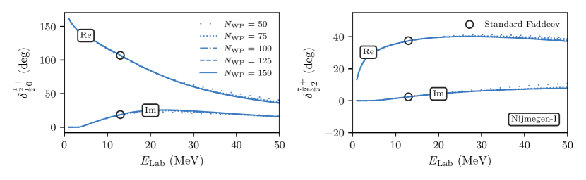
Figure 1: The $nd$ scattering phase shifts (real and imaginary parts) in the doublet and quartet spin channels of the $\frac{1}{2}^{+}$ (left panel) and $\frac{7}{2}^{+}$ (right panel) $NNN$ partial waves, respectively. Standard Faddeev results at $E_{\text{Lab}}=13$ MeV from Ref. [2]. See App. E for more on the notation.

Next to the computational cost of initially constructing $\mathbf{P}$, the cost of setting up the kernel $\mathbf{K}$ constitutes the numerical bottleneck in our current implementation of the WPCD method as it must be repeated several times. The product $\mathbf{GA}$ is trivial, which in turn makes it trivial to compute transition matrices at several different energies $E$ with the WPCD method. The product $\mathbf{C}^{T}\mathbf{PVC}$ is a product of the sparse matrix $\mathbf{P}$ with the block-diagonal matrices $\mathbf{C}^{T}$ and $\mathbf{VC}$ on either side. Note also that $\mathbf{C}$ and $\mathbf{V}$ have the same block-diagonal structure. For the product $\mathbf{A}\mathbf{K}^{n}$ we re-use the on-shell row(s) of the $\mathbf{A}\mathbf{K}^{n-1}$ matrix product computed for the $(n-1)$th term.

The (complex) on-shell transition amplitudes $U(E)$ for spin$-\frac{1}{2}$–spin-$1$ scattering constitutes a $3\times 3$ matrix. Once this matrix is computed in all relevant $NNN$ partial waves, i.e., for $\mathcal{J}\leq 17/2$ and $J\leq 3$ in our case, it is straightforward to obtain the $6\times 6$ spin-scattering matrix for describing the elastic $Nd$ scattering cross sections at kinetic energy $E_{\text{Lab}}$ in the laboratory frame of reference, see App. D-E.

II.4 Convergence with respect to $N_{\text{WP}}$

In the limit $N_{\text{WP}}\rightarrow\infty$, amplitudes computed using the WPCD method approaches results from the standard Faddeev method utilizing a plane-wave basis. This infinite limit cannot be reached in practice and all WPCD predictions that we present are based on solving Eq. (1) in a finite wave-packet basis. To analyze the convergence of predictions with respect to increasing $N_{\text{WP}}$ we computed $nd$ scattering phase shifts, shown in Fig. 1 for the doublet and quartet spin-channels in the $\mathcal{J}^{\Pi}=\frac{1}{2}^{+}$ and $\frac{7}{2}^{+}$ $NNN$ partial waves, respectively, using the Nijmegen-I $NN$ interaction [17]. For this potential there exists published results [2] from a standard Faddeev calculation at $E_{\text{Lab}}=13$ MeV and this provides a valuable benchmark to ensure the correctness of our implementation. Detailed numerical inspection of the results reveal that we recover standard Faddeev results for all imaginary and real parts of the $NNN$ phase shifts for $\mathcal{J}^{\Pi}\leq\frac{7}{2}^{\pm}$ within $\sim 1\%$ using $N_{\text{WP}}\gtrsim 125$ wave packets. We also observe that the magnitude of the imaginary part of the phase shifts is $|\text{Im}(\delta)|\lesssim 10^{-2}$ degrees for scattering energies below the deuteron breakup threshold. The convergence with increasing $N_{\text{WP}}$ is rather slow however, which is to be expected since a packetized basis corresponds to a coarse grained continuum representation across a wide range of energies simultaneously. In Fig. 1 it is nevertheless clear that the WPCD method yields highly accurate scattering phase shifts for $E_{\text{Lab}}\lesssim 50$ MeV already for $N_{\text{WP}}\gtrsim 75$. See App. E for further information about how we computed phase shifts from the partial-wave scattering amplitudes $U$.

Predicting scattering observables is more interesting than scattering phase shifts since they are directly comparable to experimental data. To benchmark our WPCD computation of observables we compare with the results from a standard Faddeev calculation [2] of the neutron analyzing power $A_{y}(n)$ at $E_{\text{Lab}}=35$ MeV using the Nijmegen-I $NN$ potential, see Fig. 2. For the WPCD-calculations we varied the number of wave packets between $50\leq N_{\text{WP}}\leq 150$. The convergence pattern is very similar to the one we observed for the phase shifts and for $N_{\text{WP}}\gtrsim 125$ we hence claim convergence for this observable. Also in this calculation we included $NNN$ partial-waves with $\mathcal{J}^{\Pi}\leq\frac{17}{2}^{\pm}$ and $NN$ channels with $J\leq 3$.

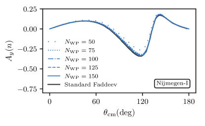
Figure 2: The neutron analyzing power $A_{y}(n)$ at $E_{\text{Lab}}=35$ MeV versus c.m. scattering angle $\theta_{\text{cm}}$ using the Nijmegen-I $NN$ potential. The WPCD prediction approaches the standard Faddeev result [2] with an increasing number of wave-packets $N_{\text{WP}}$ and they overlap for $N_{\text{WP}}\gtrsim 125$.

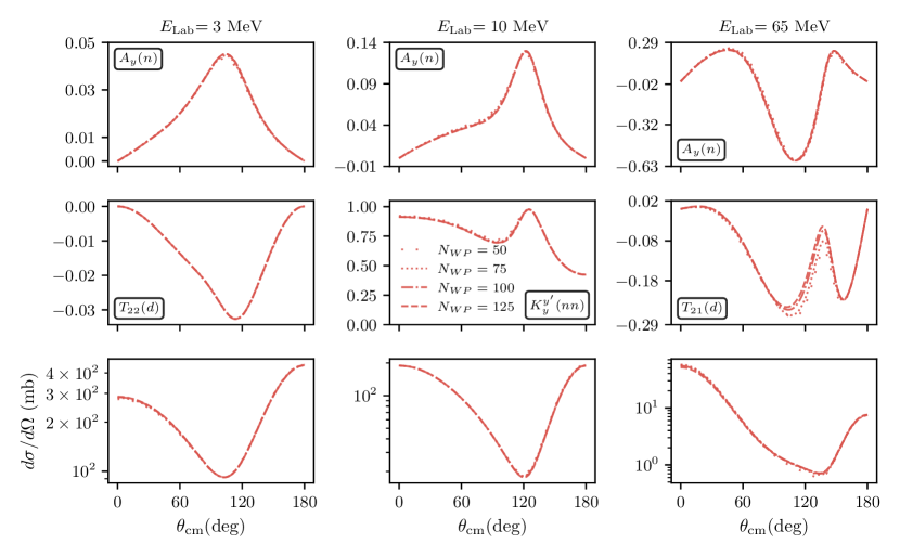
Figure 3: The convergence of WPCD predictions for typical elastic $nd$ differential scattering cross sections and polarization observables for increasing neutron scattering energies with respect to an increasing number of wave packets using the Idaho-N3LO $NN$ interaction [18].

To further assess the convergence of the WPCD method with respect to $N_{\text{WP}}$, we study a range of vector ($A$) and spherical tensor ($T$) analyzing powers, spin transfer coefficients ($K)$, and differential cross sections for $50\leq N_{\text{WP}}\leq 125$ at $E_{\text{Lab}}=3,10,65$ MeV using the well-known chiral Idaho-N3LO interaction [18], see Fig. 3.

With this result we can establish that for most elastic $nd$ scattering observables it is indeed enough to employ $N_{\text{WP}}\gtrsim 75$ wave packets to obtain sufficiently accurate predictions for $E_{\text{Lab}}\lesssim 70$ MeV. If one can tolerate a WPCD method-error comparable to typical experimental errors of $Nd$ scattering data, then even $N_{\text{WP}}\approx 50$ will be enough for most low-energy $Nd$ predictions. Note that the number of wave packets dramatically impact the computational cost of the WPCD calculations since this scales as $\sim N_{\text{WP}}^{4}$. Also, solving for all amplitudes with $E_{\text{Lab}}\lesssim 100$ MeV is merely $\sim 2$ times slower than solving at a single scattering energy.

In Fig. 3 the wave-packet convergence of the tensor analyzing power $T_{21}$ stands out and exhibits a noticeable sensitivity to $N_{\text{WP}}$. This observable is known to also depend more strongly on $J_{\text{max}}=4$ contributions of the $NN$ interaction [2]. Observables that depend on finer details of the nuclear interaction will exhibit a slower convergence with respect to increasing $N_{\text{WP}}$, due to the coarse-graining of WPCD. Fortunately, poorly converging predictions can be identified straightforwardly. We explored various modifications to the wave-packet distributions, e.g., increasing the density of wave-packets in the vicinity of the scattering energy, but this did not lead to any clear improvements.

III Predicting $nd$-scattering cross sections using $\text{N2LO}_{\text{opt}}$

In this section we present selected low-energy and elastic $nd$ cross sections using the $\text{N2LO}_{\text{opt}}$ $NN$ interaction and compare with neutron-deuteron ($nd$) as well as proton-deuteron ($pd$) data. We can neglect method uncertainties since we employ $N_{\text{WP}}=125$ wave-packets for all predictions, unless otherwise stated.

The world database of $Nd$ scattering cross sections contains mostly $pd$ data from experiments with either polarized or non-polarized proton or deuteron beams. Indeed, $nd$ scattering is difficult to perform. It is challenging to manipulate and focus electrically neutral particles. The neutron itself is unstable and does not make for a suitable target material on its own. Neutron detectors are also less efficient compared charged-particle detectors. Theoretically, we have the opposite situation. It is typically much easier to compute $Nd$ scattering cross sections without a Coulomb interaction  [36, 37]. Fortunately, Coulomb effects are only significant at low energies, e.g., below the deuteron breakup threshold, and for extremal scattering angles. As such, in most kinematic regions $pd$ scattering data can be compared with theoretical $Nd$ scattering results without any Coulomb interaction. We will therefore use $pd$ data in case $nd$ data does not exist or is very scarce. To be clear, we do not include any Coulomb effects in our calculations. One can extend the WPCD method to incorporate such effects. Indeed, the challenge of treating a long-range interaction for small momenta is alleviated when using a square-integrable Coulomb wave-packet basis [14].

In Fig. 4 we show our predictions for the total $nd$ scattering cross section with the $\text{N2LO}_{\text{opt}}$ interaction. The reproduction of experimental $nd$ data is excellent up to $E_{\text{Lab}}\approx 70$ MeV. At this point we also begin to see a difference between the $N_{\text{WP}}=100$ and $N_{\text{WP}}=125$ calculations. At $E_{\text{Lab}}>70$ MeV, the inclusion of $J>3$ $NN$-channels will have a percent-level effect on the predictions. We also note that $E_{\text{Lab}}\approx 70$ MeV corresponds to a relative momentum $q\approx 240$ MeV of the incident neutron. This translates to a $NN$ scattering energy of 125 MeV in the lab frame. The $\text{N2LO}_{\text{opt}}$ goodness-of-fit measure , i.e., the $\chi^{2}/N_{\text{datum}}$ with respect to $NN$ scattering data, is $\approx 1$ up to 125 MeV scattering energy. As such, it is reasonable to expect a gradual deterioration of the predictive power for $E_{\text{Lab}}>70$ MeV.

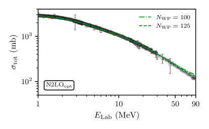
Figure 4: Total $nd$ cross sections computed using the WPCD method and the optical theorem, see e.g. Ref. [38]. Experimental $nd$ data retrieved via EXFOR [39].

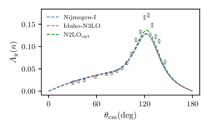
Figure 5: The neutron analyzing power $A_{y}(n)$ at $E_{\text{Lab}}=10$ MeV computed using the WPCD method with $N_{\text{WP}}=125$ wave-packets. At the maximum, the top dashed line is the $\text{N2LO}_{\text{opt}}$ result. Experimental $nd$ data from Ref. [40].

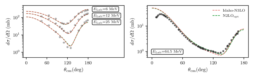
Figure 6: The differential cross section for elastic $nd$ scattering computed using the WPCD method with $N_{\text{WP}}=125$ wave-packets. The experimental $nd$ data (empty markers) at $E_{\text{Lab}}=6,12,25$ MeV in the left panel are from Ref. [41] and the $pd$ data (filled markers) at $E_{\text{Lab}}=64.5$ MeV in the right panel are from Ref. [42]. For $E_{\text{Lab}}=64.5$ MeV (right panel) the Idaho-N3LO predicts a slightly smaller cross section at the minimum.

At energies below $E_{\text{Lab}}\approx 50-100$ MeV the effects of $NNN$ interactions are typically smaller [22, 27, 43, 32], and the bulk of low-energy $Nd$ scattering observables can be described quite well using only $NN$ interactions. However, there exist a few scattering observables at these low energies that exhibit discrepancies due to missing $NNN$ forces and (or) possibly fine-tuning effects, e.g., low-energy analyzing powers, the high-energy differential cross section minimum, and the $nd$ doublet scattering length. The latter is known to correlate with the triton binding energy via the well-known Phillips line [44]. The $nd$ scattering length can be computed using a bound-state formulation of the Faddeev equations [45] or via numerical extrapolation of the scattering amplitude to $q\rightarrow 0$. Unfortunately, this limit is challenging to reach in the WPCD method with the Chebyshev distribution we employ. Resorting to a basis with an increased number wave-packets at small momenta will of course remedy this. However, to simultaneously maintain accurate scattering amplitudes for higher scattering energies will result in a needlessly large basis size.

The prediction of the neutron analyzing power $A_{y}(n)$ at $E_{\text{Lab}}=10$ MeV with $\text{N2LO}_{\text{opt}}$ is shown in Fig. 5. For comparison we also include WPCD results using the Idaho-N3LO and Nijmegen-I potentials. All three potentials yield virtually the same result and the discrepancy with respect to ${}^{2}H(n,n)^{2}H$ data [40] at the c.m. scattering angles $\theta_{cm}\approx 120^{\circ}$, known as the $A_{y}$-puzzle [30], persists also with $\text{N2LO}_{\text{opt}}$. There is some tendency of a slight increase using this latter potential, but this is certainly not significant on an absolute scale. This result reflects that the low-energy interaction in the ${}^{3}P$-channels of $\text{N2LO}_{\text{opt}}$, to which we know that $A_{y}$ is most sensitive [30], are similar to the ones in Idaho-N3LO and Nijmegen-I. A detailed calculation [32] to very high chiral orders suggests that the inclusion of leading $NNN$ forces does not resolve the $A_{y}$-puzzle. Instead, there are hints that the $A_{y}$-puzzle could be resolved with sub-leading $NNN$ forces [43]. Alternatively, the $A_{y}$ puzzle might vanish in a simultaneous $NN$+$NNN$ analysis conditioned on $NN$ and $Nd$ scattering data and informed by model discrepancies such as the truncation error in effective field theory.

Low-energy $nd$ differential cross-section data is very well reproduced by $\text{N2LO}_{\text{opt}}$, see the left panel of Fig. 6, and the results are identical to what is obtained using the Idaho-N3LO potential. At higher energies, however, there are some discrepancies with respect to data and the two employed potentials differ slightly in the vicinity of the cross section minimum. A previous study [31] concluded that the effects of $NNN$ interactions are expected to be particularly noticeable in this angular region. Although the $\text{N2LO}_{\text{opt}}$ prediction lies marginally closer to the experimental data at $\theta_{\text{cm}}\approx 120^{\circ}$ the shape of the differential cross section is not correct.

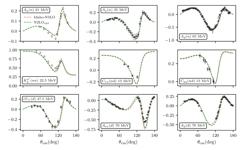
Figure 7: Spin observables for elastic $nd$ scattering computed using the WPCD method with $N_{\text{WP}}=125$ wave-packets and the $\text{N2LO}_{\text{opt}}$ and the Idaho-N3LO potentials. The experimental $nd$ data (empty markers) at $E_{\text{Lab}}=21,22.5$ and 65 MeV are from Refs. [46], [47], and [48], respectively. The $pd$ data (filled markers) at $E_{\text{Lab}}=13,35,47.5,65$ and 70 MeV are from Refs. [49], [50], [51], [42], and [52], respectively. See the main text for detailed discussion.

In Fig. 7 we show a range of spin observables for $E_{\text{Lab}}=13-70$ MeV. Overall, $\text{N2LO}_{\text{opt}}$ and Idaho-N3LO describe the data rather well in this energy region and the two different potentials produce virtually identical results. In the top row of Fig. 7 we present $A_{y}(n)$ for increasing values of $E_{\text{Lab}}$. It is well known that at energies below $\sim 30$ MeV nearly all $NN$ interactions fail to describe the data for this observable [46]. As was discussed above, the $\text{N2LO}_{\text{opt}}$ interaction does not remedy the puzzle. Nevertheless, careful inspection reveals that the predictions for $A_{y}$ at $E_{\text{Lab}}=21$ MeV fits the data slightly better at large scattering angles when using $\text{N2LO}_{\text{opt}}$. Unfortunately, discrepancies with respect to data persists for small scattering angles, i.e., at the minimum value of $A_{y}$. In the second row of Fig. 7 we present low-energy neutron-to-neutron spin transfer ($K$) and neutron-to-deuteron correlation ($C$) observables. Previous studies [53] have found that the $K_{y}^{y^{\prime}}$ spin transfer is most sensitive to the structure of the $NN$ interaction in the ${}^{3}S_{1}$–${}^{3}D_{1}$ and ${}^{1}P_{1}$ channels. Since Idaho-N3LO and $\text{N2LO}_{\text{opt}}$ have very similar $NN$ phase shifts below $E_{\text{Lab}}=100$ MeV in these channels it is not surprising to recover very similar results also for these observables. Of course, the former potential incorporates higher-order long- and short-range physics that modify the off-shell structure of the potential, but this does not appear alter the predictions much. Regarding the tensor analyzing powers presented in the third row, the discrepancy between theory and data for $A_{xx}(d)$ at $\theta_{\text{cm}}\approx 150^{\circ}$ persists for both potentials. Inclusion of modern $NNN$ forces does not resolve this [43].

IV Summary and outlook

In this work we presented a framework that allows to solve the Faddeev equations for elastic $Nd$ scattering using a newly developed code based on the WPCD method. We analyzed the convergence of the WPCD method, applied to chiral potentials, with respect to the number of basis wave packets $N_{\text{WP}}$. We find negligible method errors when using $N_{\text{WP}}=125$ in the regime $E_{\text{Lab}}\lesssim 70$ MeV.

We studied different $nd$ scattering observables up to $E_{\text{Lab}}=70$ MeV with the $\text{N2LO}_{\text{opt}}$ $NN$ interaction and find a good overall reproduction of the scattering data. However, the $A_{y}$-puzzle remains unsolved when applying the $\text{N2LO}_{\text{opt}}$ interaction. Compared to the Nijmegen-I and Idaho-N3LO $NN$ interactions, we detect a minor increase in the maximum of the theoretical predictions of this observable at low energies. For other cross sections we find a good reproduction of experimental data and the results are virtually indistinguishable from the Idaho-N3LO interaction. The $\text{N2LO}_{\text{opt}}$ interaction prediction for $d\sigma/d\Omega$ at $E_{\text{Lab}}=64.5$ MeV is slightly closer to the data at the differential cross section minimum. This observable is typically associated with an increased sensitivity to $NNN$ interactions.

Next, we will explore discretized bases with a different number of wave-packets for the $p$ and $q$ momenta, make predictions for breakup cross sections, and incorporate $NNN$ interactions in our calculations. Although some observables, that depend sensitively on finer details of the nuclear interaction, require more wave-packets to be accurately resolved one can obtain sufficiently accurate predictions for the vast majority of low-energy $Nd$ cross sections with $N_{\text{WP}}\approx 50$ wave packets, which will help to reduce the computational demands of the calculations to a level that allows a study of $Nd$ scattering observables within a statistical analysis. Specifically, in the near term we plan to employ WPCD predictions to sample Bayesian posterior predictive distributions for $Nd$ scattering. Work in this direction, using frequentist methods, was also initiated in [54]. In the longer perspective, emulator methods based on perturbation theory [55] or eigenvector continuation [56] promise an efficient method for fast and accurate emulation of scattering observables [57, 58, 59, 60] and will open new ways to systematically incorporate $Nd$ scattering observables in the construction and fitting process of next-generation $NN$ and $NNN$ interactions.

Appendix A Partial-wave decomposition of the permutation operator in a plane-wave basis

In this section we present the permutation operator $\hat{P}_{123}$ in a plane-wave partial-wave basis. The permutation operator $\hat{P}_{ijk}=\hat{P}_{ij}\hat{P}_{jk}$ performs two pairwise interchanges of particles: first $j\leftrightarrow k$ followed by $i\leftrightarrow j$. Our derivation follows the steps presented in [29], as well as the notation and convention for the Jacobi momenta $\bm{p}$ and $\bm{q}$. For this section we will use the indexing ($ij$) to denote the $ij$-pair system for the sake of clarity, rather than the odd-man-out notation. To complement [29], we use the $(12)$-subsystem as our initial states upon which the permutation operator acts. One can show that all representations of $\hat{P}_{123}$ are invariant under change of reference system. Furthermore, one can show [29, 1] that for a basis that is antisymmetric under exchange of particles 2 and 3, we have $\langle\hat{P}_{123}\rangle=\langle\hat{P}_{132}\rangle$. This allows us to express projections of $\hat{P}$ in Eq. (1) simply as $\langle\hat{P}\rangle=\langle 1+2\hat{P}_{123}\rangle$.

Our starting point is the following overlap

$$\begin{split}\prescript{}{12}{\langle}p^{\prime}q^{\prime};\alpha^{\prime}|\hat{P}_{123}|pq;\alpha\rangle_{12}&=\prescript{}{12}{\langle}p^{\prime}q^{\prime};\alpha^{\prime}|\hat{P}_{12}\hat{P}_{23}|pq;\alpha\rangle_{12}\\ &=\prescript{}{12}{\langle}p^{\prime}q^{\prime};\alpha^{\prime}|pq;\alpha\rangle_{23}\>.\end{split}$$ (12)

which, projected in a partial-wave basis, becomes (note that that magnetic quantum numbers $m_{\mathcal{J}}$ and $m_{\mathcal{T}}$ are implied in $|\alpha\rangle$)

$$\begin{split}\prescript{}{12}{\langle p^{\prime}q^{\prime};\alpha^{\prime}}|pq;\alpha\rangle_{23}&=\sum_{\mathcal{L}\mathcal{S}}\sum_{\mathcal{L}^{\prime}\mathcal{S}^{\prime}}\sqrt{\hat{J}^{\prime}\hat{j}^{\prime}\hat{\mathcal{L}}^{\prime}\hat{\mathcal{S}}^{\prime}}\sqrt{\hat{J}\hat{j}\hat{\mathcal{L}}\hat{\mathcal{S}}}\\ &\hphantom{=}\times\begin{Bmatrix}L^{\prime}&S^{\prime}&J^{\prime}\\ l^{\prime}&\frac{1}{2}&j^{\prime}\\ \mathcal{L}^{\prime}&\mathcal{S}^{\prime}&\mathcal{J}^{\prime}\end{Bmatrix}\begin{Bmatrix}L&S&J\\ l&\frac{1}{2}&j\\ \mathcal{L}&\mathcal{S}&\mathcal{J}\end{Bmatrix}\\ &\hphantom{=}\times\sum_{m_{\mathcal{L}}m_{\mathcal{S}}}\sum_{m_{\mathcal{L}^{\prime}}m_{\mathcal{S}^{\prime}}}C_{\mathcal{L}^{\prime}m_{\mathcal{L}^{\prime}},\mathcal{S}^{\prime}m_{\mathcal{S}}^{\prime}}^{\mathcal{J}^{\prime}m_{\mathcal{J}^{\prime}}}C_{\mathcal{L}m_{\mathcal{L}},\mathcal{S}m_{\mathcal{S}}}^{\mathcal{J}m_{\mathcal{J}}}\\ &\hphantom{=}\times\prescript{}{12}{\langle}p^{\prime}q^{\prime};L^{\prime}l^{\prime}\mathcal{L}^{\prime}m_{\mathcal{L}^{\prime}}|pq;Ll\mathcal{L}m_{\mathcal{L}}\rangle_{23}\\ &\hphantom{=}\times\prescript{}{12}{\langle}(S^{\prime}\frac{1}{2})\mathcal{S}^{\prime}m_{\mathcal{S}^{\prime}}|(S\frac{1}{2})\mathcal{S}m_{\mathcal{S}}\rangle_{23}\\ &\hphantom{=}\times\prescript{}{12}{\langle}(T^{\prime}\frac{1}{2})\mathcal{T}^{\prime}m_{\mathcal{T}^{\prime}}|(T\frac{1}{2})\mathcal{T}m_{\mathcal{T}}\rangle_{23}\>,\\ \end{split}$$ (13)

where the spin and isospin recouplings are given by the Wigner-6j symbols,

$$\begin{split}&\prescript{}{12}{\langle}(S^{\prime}\frac{1}{2})\mathcal{S}^{\prime}m_{\mathcal{S}^{\prime}}|(S\frac{1}{2})\mathcal{S}m_{\mathcal{S}}\rangle_{23}\\ =&\delta_{\mathcal{S}^{\prime}\mathcal{S}}\delta_{m_{\mathcal{S}^{\prime}}m_{\mathcal{S}}}(-1)^{S}\sqrt{\hat{S}^{\prime}\hat{S}}\begin{Bmatrix}\frac{1}{2}&\frac{1}{2}&S^{\prime}\\ \frac{1}{2}&\mathcal{S}&S\end{Bmatrix}\>.\end{split}$$ (14)

Here, $C_{l_{1}m_{1},l_{2}m_{2}}^{l_{3}m_{3}}$ denote Clebsch-Gordan coefficients and we use the notation $\hat{n}\equiv\sqrt{2n+1}$ The recoupling of orbital angular momenta are calculated using momentum-space projection in the pair-systems $(12)$ and $(23)$,

$$\begin{split}&\prescript{}{12}{\langle}p^{\prime}q^{\prime};L^{\prime}l^{\prime}\mathcal{L}^{\prime}m_{\mathcal{L}^{\prime}}|pq;Ll\mathcal{L}m_{\mathcal{L}}\rangle_{23}\\ &=\int_{0}^{\infty}\>d\bm{p}_{12}^{\prime\prime\prime}\>d\bm{q}_{12}^{\prime\prime\prime}d\bm{p}_{23}^{\prime\prime}\>d\bm{q}_{23}^{\prime\prime}\>\mathcal{Y}_{L^{\prime}l^{\prime}}^{*\mathcal{L}^{\prime}m_{\mathcal{L}^{\prime}}}(\hat{\bm{p}}_{12}^{\prime\prime\prime},\hat{\bm{q}}_{12}^{\prime\prime\prime})\\ &\hphantom{=}\times\prescript{}{12}{\langle}\bm{p}^{\prime\prime\prime}\bm{q}^{\prime\prime\prime}|\bm{p}^{\prime\prime}\bm{q}^{\prime\prime}\rangle_{23}\>\mathcal{Y}_{Ll}^{\mathcal{L}m_{\mathcal{L}}}(\hat{\bm{p}}_{23}^{\prime\prime},\hat{\bm{q}}_{23}^{\prime\prime})\\ &\hphantom{=}\times\left[\frac{\delta(p^{\prime}-p^{\prime\prime\prime})}{p^{\prime}p^{\prime\prime\prime}}\frac{\delta(q^{\prime}-q^{\prime\prime\prime})}{q^{\prime}q^{\prime\prime\prime}}\right]_{12}\\ &\hphantom{=}\times\left[\frac{\delta(p^{\prime\prime}-p)}{p^{\prime\prime}p}\frac{\delta(q^{\prime\prime}-q)}{q^{\prime\prime}q}\right]_{23}\>,\\ \end{split}$$ (15)

where the hat-notation on vectors indicate unit vectors, and we introduced the coupled spherical harmonics,

$$\mathcal{Y}_{l_{1}l_{2}}^{l_{3}m_{3}}(\hat{\bm{a}},\hat{\bm{b}})=\sum_{m_{1}m_{2}}C_{l_{1}m_{1},l_{2}m_{2}}^{l_{3}m_{3}}Y_{l_{1}m_{1}}(\hat{\bm{a}})Y_{l_{2}m_{2}}(\hat{\bm{b}})\>,$$ (16)

and where $Y_{lm}(\hat{\bm{a}})$ are the spherical harmonics. Note that we use the Condon-Shortley phase factor. Furthermore we use proper normalization of the spherical harmonics, such that numerical evaluation is performed in terms of the associated Legendre polynomials as $Y_{lm}(\hat{\bm{a}})=e^{im\theta}P_{l}^{m}(\cos(\phi))$ where $\hat{\bm{a}}=(\theta,\phi)$.

The inner product of Jacobi momenta,

$$\prescript{}{12}{\langle}\bm{p}^{\prime\prime\prime}\bm{q}^{\prime\prime\prime}|\bm{p}^{\prime\prime}\bm{q}^{\prime\prime}\rangle_{23}=\delta(\bm{p}^{\prime\prime\prime}_{12}-\bm{p}^{\prime\prime}_{12})\delta(\bm{q}^{\prime\prime\prime}_{12}-\bm{q}^{\prime\prime}_{12})\>,$$ (17)

can be resolved using the identities $\bm{p}^{\prime\prime}_{12}=-\frac{1}{2}\bm{p}_{23}^{\prime\prime}+\frac{3}{4}\bm{q}_{23}^{\prime\prime}$ and $\bm{q}^{\prime\prime}_{12}=-\bm{p}_{23}^{\prime\prime}-\frac{1}{2}\bm{q}_{23}^{\prime\prime}$, from which we can define four variables that fulfil momentum conservation,

$$\begin{split}\prescript{}{12}{\langle}\bm{p}^{\prime\prime\prime}\bm{q}^{\prime\prime\prime}|\bm{p}^{\prime\prime}\bm{q}^{\prime\prime}\rangle_{23}&=\delta(\bm{p}_{23}^{\prime\prime}-\bm{\bar{p}})\delta(\bm{q}_{23}^{\prime\prime}-\bm{\bar{q}})\\ &=\delta(\bm{p}_{12}^{\prime\prime\prime}-\bm{\tilde{p}})\delta(\bm{q}_{12}^{\prime\prime\prime}-\bm{\tilde{q}})\\ &=\delta(\bm{p}_{12}^{\prime\prime\prime}-\bm{\pi}^{\prime})\delta(\bm{p}_{23}^{\prime\prime}-\bm{\pi})\\ &=\delta(\bm{q}_{12}^{\prime\prime\prime}-\bm{\kappa}^{\prime})\delta(\bm{q}_{23}^{\prime\prime}-\bm{\kappa})\>.\end{split}$$ (18)

Here, we also defined (in the pair-system $(12)$)

$$\begin{split}&\left.\begin{cases}\bm{\bar{p}}&\equiv-\frac{1}{2}\bm{p}_{12}^{\prime\prime\prime}-\frac{3}{4}\bm{q}_{12}^{\prime\prime\prime}\\ \bm{\bar{q}}&\equiv\bm{p}_{12}^{\prime\prime\prime}-\frac{1}{2}\bm{q}_{12}^{\prime\prime\prime}\end{cases}\right\}\>,\quad\left.\begin{cases}\bm{\tilde{p}}&\equiv-\frac{1}{2}\bm{p}_{23}^{\prime\prime}+\frac{3}{4}\bm{q}_{23}^{\prime\prime}\\ \bm{\tilde{q}}&\equiv-\bm{p}_{23}^{\prime\prime}-\frac{1}{2}\bm{q}_{23}^{\prime\prime}\end{cases}\right\}\>,\\ &\left.\begin{cases}\bm{\pi}&\equiv-\frac{1}{2}\bm{q}_{23}^{\prime\prime\prime}-\bm{q}_{12}^{\prime\prime}\\ \bm{\pi}^{\prime}&\equiv\frac{1}{2}\bm{q}_{12}^{\prime\prime}+\bm{q}_{23}^{\prime\prime\prime}\end{cases}\right\}\>,\quad\left.\begin{cases}\bm{\kappa}&\equiv\frac{2}{3}\bm{p}_{23}^{\prime\prime\prime}+\frac{4}{3}\bm{p}_{12}^{\prime\prime}\\ \bm{\kappa}^{\prime}&\equiv-\frac{4}{3}\bm{p}_{23}^{\prime\prime\prime}-\frac{2}{3}\bm{p}_{12}^{\prime\prime}\end{cases}\right\}\>.\end{split}$$ (19)

Note that the exact form of these relations depend on the choice of pair-system. See [29] for a summary of three-body kinematics.

Choosing to conserve $(\bm{\bar{p}},\bm{\bar{q}})$ will restrict the bra-momenta of an operator to the right of the permutation operator in the Faddeev equation due to the ensuing delta-functions (used in e.g. [29, 2]). Likewise, $(\bm{\tilde{p}},\bm{\tilde{q}})$ will restrict the ket-momenta of an operator to the left, while $(\bm{\kappa},\bm{\kappa}^{\prime})$ will restrict $p$ of operators on both sides, and lastly $(\bm{\pi},\bm{\pi}^{\prime})$ will restrict $q$ on both sides (used in e.g. [61, 62]). In this work we have followed [29] and conserve $(\bm{\bar{p}},\bm{\bar{q}})$. From this point on we drop the $(12)$ subscript on momenta and get

$$\begin{split}\prescript{}{12}{\langle}p^{\prime}q^{\prime};L^{\prime}l^{\prime}\mathcal{L}^{\prime}m_{\mathcal{L}^{\prime}}|pq;Ll\mathcal{L}m_{\mathcal{L}}\rangle_{23}&=\int_{0}^{\infty}d\bm{p}^{\prime\prime\prime}\>d\bm{q}^{\prime\prime\prime}\\ &\hphantom{=}\times\mathcal{Y}_{L^{\prime}l^{\prime}}^{*\mathcal{L}^{\prime}m_{\mathcal{L}^{\prime}}}(\hat{\bm{p}}^{\prime\prime\prime},\hat{\bm{q}}^{\prime\prime\prime})\\ &\hphantom{=}\times\mathcal{Y}_{Ll}^{\mathcal{L}m_{\mathcal{L}}}(\hat{\bm{\bar{p}}},\hat{\bm{\bar{q}}})\\ &\hphantom{=}\times\frac{\delta(\bar{p}-p)}{\bar{p}p}\frac{\delta(\bar{q}-q)}{\bar{q}q}\>,\end{split}$$ (20)

where $\bar{p}=|\bar{\bm{p}}|$ and $\bar{q}=|\bar{\bm{q}}|$. The integral is invariant under rotations, making it proportional to $\delta_{\mathcal{L}^{\prime}\mathcal{L}}\delta_{m_{\mathcal{L}^{\prime}}m_{\mathcal{L}}}$. This invariance allows us to simply average out $m_{\mathcal{L}}$, giving a factor $\frac{1}{2\mathcal{L}+1}$. We now have freedom in the choice of axes. Choosing $\hat{z}\parallel\bm{\hat{p}}^{\prime\prime\prime}$ and the polar angle of $\hat{\bm{q}}^{\prime\prime\prime}$ to zero, we can simplify a spherical harmonic: $Y_{L^{\prime}m_{L^{\prime}}}(\hat{\bm{p}}^{\prime\prime\prime})=\sqrt{\frac{\hat{L}^{\prime}}{4\pi}}\delta_{m_{L^{\prime}}0}$. By solving the remaining angular integrals we are left with

$$\begin{split}\prescript{}{12}{\langle}p^{\prime}q^{\prime};L^{\prime}l^{\prime}\mathcal{L}^{\prime}|pq;Ll\mathcal{L}\rangle_{23}&=8\pi^{2}\frac{\delta_{\mathcal{L}^{\prime}\mathcal{L}}}{\hat{\mathcal{L}}}\int_{-1}^{+1}dx\\ &\hphantom{=}\times\frac{\delta(\bar{p}-p)}{\bar{p}p}\frac{\delta(\bar{q}-q)}{\bar{q}q}\\ &\hphantom{=}\times\sum_{m_{\mathcal{L}}}\mathcal{Y}_{L^{\prime}l^{\prime}}^{*\mathcal{L}^{\prime}m_{\mathcal{L}^{\prime}}}(\hat{\bm{p}}^{\prime\prime\prime},\hat{\bm{q}}^{\prime\prime\prime})\\ &\hphantom{=}\times\mathcal{Y}_{Ll}^{\mathcal{L}m_{\mathcal{L}}}(\hat{\bar{\bm{p}}},\hat{\bar{\bm{q}}})\>,\end{split}$$ (21)

where vectors are functions of $(p^{\prime},q^{\prime},x)$ and $x=\cos(\phi)$ (the angle from $\bm{q}^{\prime\prime\prime}$ to $\bm{p}^{\prime\prime\prime}$). Notice the change in notation of states on the left-hand side as we averaged with respect to $m_{\mathcal{L}}$. Inserting Eq. (21) and Eq. (16) back into Eq. (13) gives

$$\prescript{}{12}{\langle}p^{\prime}q^{\prime};\alpha^{\prime}|\hat{P}_{123}|pq;\alpha\rangle_{12}=\int_{-1}^{1}dx\>G_{\alpha\alpha^{\prime}}(p^{\prime},q^{\prime},x)\frac{\delta(\bar{p}-p)}{\bar{p}p}\frac{\delta(\bar{q}-q)}{\bar{q}q}\>,$$ (22)

with the geometrical function $G_{\alpha\alpha^{\prime}}(p^{\prime},q^{\prime},x)$ in a form that is straightforward to implement algorithmically,

$$\begin{split}G_{\alpha\alpha^{\prime}}(p^{\prime},q^{\prime},x)=\delta_{\mathcal{J}^{\prime}\mathcal{J}}\delta_{\mathcal{T}^{\prime}\mathcal{T}}&\sum_{\mathcal{L}\mathcal{S}}\sqrt{\hat{J}^{\prime}\hat{J}}\sqrt{\hat{j}^{\prime}\hat{j}}\hat{\mathcal{S}}\begin{Bmatrix}L^{\prime}&S^{\prime}&J^{\prime}\\ l^{\prime}&\frac{1}{2}&j^{\prime}\\ \mathcal{L}&\mathcal{S}&\mathcal{J}\end{Bmatrix}\begin{Bmatrix}L&S&J\\ l&\frac{1}{2}&j\\ \mathcal{L}&\mathcal{S}&\mathcal{J}\end{Bmatrix}(-1)^{S}\sqrt{\hat{S}^{\prime}\hat{S}}\begin{Bmatrix}\frac{1}{2}&\frac{1}{2}&S^{\prime}\\ \frac{1}{2}&\mathcal{S}&S\end{Bmatrix}(-1)^{T}\sqrt{\hat{T}^{\prime}\hat{T}}\begin{Bmatrix}\frac{1}{2}&\frac{1}{2}&T^{\prime}\\ \frac{1}{2}&\mathcal{T}&T\end{Bmatrix}\\ \times\frac{8\pi^{2}}{\sqrt{4\pi}}&\sum_{m_{\mathcal{L}}m_{L}m_{l}}C_{L^{\prime}0,lm_{\mathcal{L}}}^{\mathcal{L}m_{\mathcal{L}}}C_{Lm_{L},lm_{l}}^{\mathcal{L}m_{\mathcal{L}}}P_{L}^{m_{L}}(\cos(\theta_{1}))P_{l}^{m_{l}}(\cos(\theta_{2}))(-1)^{m_{\mathcal{L}}}P_{l^{\prime}}^{m_{\mathcal{L}}}(x)\>,\quad m_{\mathcal{L}}\equiv m_{L}+m_{l}\>,\\ \end{split}$$ (23)

and where we defined

$$\begin{split}\cos(\theta_{1})&\equiv\frac{|\bar{\bm{p}}_{z}|}{\bar{p}}=\frac{-\frac{1}{2}p^{\prime}-\frac{3}{4}q^{\prime}x}{\bar{p}}\>,\\ \cos(\theta_{2})&\equiv\frac{|\bar{\bm{q}}_{z}|}{\bar{q}}=\frac{p^{\prime}-\frac{1}{2}q^{\prime}x}{\bar{q}}\>.\end{split}$$ (24)

and where we used $m_{L^{\prime}}=0$. Given that we have $\mathcal{S}=\mathcal{S}^{\prime}$, $m_{\mathcal{S}}=m_{\mathcal{S}^{\prime}}$, $\mathcal{L}=\mathcal{L}^{\prime}$, and $m_{\mathcal{L}}=m_{\mathcal{L}^{\prime}}$, we used the orthogonality of Clebsch-Gordan coefficients,

$$\sum_{m_{1}m_{2}}C_{l_{1}m_{1},l_{2}m_{2}}^{l_{3}^{\prime}m_{3}^{\prime}}C_{l_{1}m_{1},l_{2}m_{2}}^{l_{3}m_{3}}=\delta_{l_{3}^{\prime}l_{3}}\delta_{m_{3}^{\prime}m_{3}}\>.$$ (25)

to set $\mathcal{J}^{\prime}=\mathcal{J}$ and $m_{\mathcal{J}}=m_{\mathcal{J}^{\prime}}$.

Previously, in [61] the angular dependence in $G_{\alpha\alpha^{\prime}}(p^{\prime},q^{\prime},x)$ was evaluated separately from the recoupling terms. This allows pre-calculation of the geometric recouplings before doing the angular integration. However, it turns out that keeping the angular dependence as above is both more numerically efficient and stabler with higher $l$ and $L$ [29]. As this function is the most computationally costly part of evaluating the integral of Eq. (22), we mention some key optimizations one can use.

The simplest and most effective optimization is to calculate $G_{\alpha\alpha^{\prime}}(p^{\prime},q^{\prime},x)$ and store it in the computer memory in its entirety. From a computational viewpoint the function is 5-dimensional, which is still storable in the computer memory for the basis sizes and number of quadrature points we typically require.

Regardless of whether prestorage of $G_{\alpha\alpha^{\prime}}(p^{\prime},q^{\prime},x)$ is possible, we still wish to speed up the calculation of $G_{\alpha\alpha^{\prime}}(p^{\prime},q^{\prime},x)$. To this end, everything before the second sum in Eq. (23) (i.e. all geometric recoupling) can easily be precalculated to improve computational performance. The second summation can be sped up by prestoring the three Legendre polynomials individually, which is usually still manageable and quite fast.

Appendix B Projecting operators to the wave-packet basis

In this section we present the expressions we employ for projecting operators to a wave-packet basis. Although Eq. (4) provides a definition of a three-body wave packet, it is written explicitly for plane-wave states. Identically, and in general, any three-body wave packet $|Y_{ij}\rangle$ (where we omit partial-wave indexing) can be defined from continuum states $|\omega_{p}\rangle$ and $|\omega_{q}\rangle$ of some operator (e.g. $\hat{p}$, $\hat{h}_{0}$, or $\hat{h}_{1}$) with Jacobi momenta $p\in\mathcal{D}_{i}$ and $q\in\bar{\mathcal{D}}_{j}$,

$$Y_{ij}=\frac{1}{N_{ij}}\int_{\mathcal{D}_{i},\bar{\mathcal{D}}_{j}}dp\>p\>dq\>q\>f(p)\bar{f}(q)|\omega_{p},\omega_{q}\rangle\>,$$ (26)

where $N_{ij}$ is the wave-packet normalization constant, and $f(p)$ and $\bar{f}(q)$ are the weighting functions defined in Sec. II.2. The wave packet can be projected onto the continuum basis straightforwardly,

$$\begin{split}\langle\omega_{p},\omega_{q}|Y_{ij}\rangle&=\frac{1}{N_{ij}}\int_{\mathcal{D}_{i},\bar{\mathcal{D}}_{j}}dp^{\prime}p^{\prime}dq^{\prime}q^{\prime}\>f(p^{\prime})\bar{f}(q^{\prime})\\ &\hskip 56.9055pt\times\langle\omega_{p},\omega_{q}|\omega_{p^{\prime}},\omega_{q^{\prime}}\rangle\\ &=\frac{1}{N_{ij}}\frac{f(p)\bar{f}(q)}{pq}\mathds{1}_{\mathcal{D}_{i}}(p)\mathds{1}_{\bar{\mathcal{D}}_{j}}(q)\>,\end{split}$$ (27)

where $\mathds{1}_{\mathcal{D}_{i}}(p)$ is the indicator function. From this it is easy to show that $N_{ij}=\sqrt{D_{i}\bar{D}_{j}}$, where $D_{i}$($\bar{D}_{j}$) is the width of $\mathcal{D}_{i}$($\bar{\mathcal{D}}_{j}$). Note that for energy wave packets the width is expressed in energy as, for example, $D_{i}=E_{i+1}-E_{i}$ for boundaries $E_{i}$. The general form of Eq. (B.1) comes in handy for analytical derivation as it applies to both free and scattering wave packets alike.

Going back to a FWP basis, a projection of a general $NNN$ operator will look as follows,

$$\begin{split}\langle X_{i^{\prime}j^{\prime}}^{\alpha^{\prime}}|\hat{O}|X_{ij}^{\alpha}\rangle=\frac{1}{N_{i^{\prime}j^{\prime}}N_{ij}}&\int_{\mathcal{D}_{i^{\prime}j^{\prime}}}dp^{\prime}\>p^{\prime}\>dq^{\prime}\>q^{\prime}\>f^{*}(p^{\prime})\bar{f}^{*}(q^{\prime})\\ \times&\int_{\mathcal{D}_{ij}}dp\>p\>dq\>q\>f(p)\bar{f}(q)\\ \times&\langle p^{\prime}q^{\prime};\alpha^{\prime}|\hat{O}|pq;\alpha\rangle\>.\end{split}$$ (28)

B.1 Two-body free Hamiltonian

For our chosen normalization, the free $NN$ Hamiltonian is given by

$$\langle p^{\prime}q^{\prime};\alpha^{\prime}|\hat{h}_{0}|pq;\alpha\rangle=\delta_{\alpha^{\prime}\alpha}\frac{\delta(p^{\prime}-p)}{p^{2}}\frac{\delta(q^{\prime}-q)}{q^{2}}\langle p|\hat{h}_{0}|p\rangle\>.$$ (29)

Clearly, the free Hamiltonian is also diagonal in the FWP basis. Depending on the choice of wave packet, we get for the $NN$ free Hamiltonian,

$$\langle X_{i^{\prime}j^{\prime}}^{\alpha^{\prime}}|\hat{h}_{0}|X_{ij}^{\alpha}\rangle=\begin{cases}\delta_{\alpha^{\prime}\alpha}\delta_{i^{\prime}i}\delta_{j^{\prime}j}\frac{p_{i+1}^{2}+p_{i}^{2}}{2\mu_{0}},&f(p)=\sqrt{\frac{p}{\mu_{0}}}\\ \delta_{\alpha^{\prime}\alpha}\delta_{i^{\prime}i}\delta_{j^{\prime}j}\frac{p_{i+1}^{2}+p_{i+1}p_{i}+p_{i}^{2}}{6\mu_{0}},&f(p)=1\,.\end{cases}$$ (30)

B.2 The $NN$ potential

The $NN$ potential $\hat{v}$ in a $NNN$ partial-wave basis reduces to

$$\langle p^{\prime}q^{\prime};\alpha^{\prime}|\hat{v}|pq;\alpha\rangle=\delta_{\gamma^{\prime}\gamma}\delta_{\Gamma^{\prime}\Gamma}\frac{\delta(q^{\prime}-q)}{q^{2}}\langle p^{\prime}|\hat{v}_{n^{\prime}n}|p\rangle\>,$$ (31)

where $\gamma$ denotes all the quantum numbers for the third nucleon relative to the pair system, i.e., $\gamma=\{l,j\}$, $\Gamma=\{\mathcal{J},\mathcal{T}\}$ denotes the coupled $NNN$ quantum numbers, and the pair-system quantum numbers are jointly referred to as $n=\{L,S,J,T\}$. For our predictions we break total $\mathcal{T}$ isospin conservation, and the expressions below must be modified in an obvious way. We obtain the $NN$ interaction in the $NNN$ FWP-basis via Eq. (28), and easily resolving the $q$-integral,

$$\begin{split}\langle X_{i^{\prime}j^{\prime}}^{\alpha^{\prime}}|\hat{v}|X_{ij}^{\alpha}\rangle=&\frac{\delta_{\gamma^{\prime}\gamma}\delta_{\Gamma\Gamma^{\prime}}\delta_{j^{\prime}j}}{D_{i^{\prime}}D_{i}}\int_{\mathcal{D}_{i^{\prime}}}dp^{\prime}\>p^{\prime}\int_{\mathcal{D}_{i}}dp\>p\\ &\times f^{*}(p^{\prime})f(p)\langle p^{\prime}|\hat{v}_{n^{\prime}n}|p\rangle\>.\end{split}$$ (32)

This expression is straightforward to evaluate numerically using quadrature.

B.3 The permutation operator

The permutation operator $\hat{P}_{123}$ in a partial-wave basis, Eq. (22), can be inserted into Eq. (28). The delta-functions are only non-zero when the Jacobi momenta $\bar{p}$ and $\bar{q}$ fall within the bins $\mathcal{D}_{i}$ and $\bar{\mathcal{D}}_{j}$, which we express using the indicator function. Choosing momentum wave-packets gives

$$\begin{split}\langle X_{i^{\prime}j^{\prime}}^{\alpha^{\prime}}|\hat{P}_{123}|X_{ij}^{\alpha}\rangle=\frac{1}{N_{i^{\prime}j^{\prime}}N_{ij}}&\int_{\mathcal{D}_{i^{\prime}j^{\prime}}}dp^{\prime}\>p^{\prime}\>dq^{\prime}\>q^{\prime}\\ \times&\int_{-1}^{1}\>dx\>G_{\alpha\alpha^{\prime}}(p^{\prime},q^{\prime},x)\\ \times&\frac{\mathds{1}_{\mathcal{D}_{j}}(\bar{p})}{\bar{p}}\frac{\mathds{1}_{\bar{\mathcal{D}}_{j}}(\bar{q})}{\bar{q}}\>.\end{split}$$ (33)

The indicator function is discontinuous and an evaluation of Eq.(33) using Gaussian quadrature in the $p$ and $q$ momenta yields poor convergence with an increasing number of quadrature points. Therefore, we transform the integral over $p^{\prime}$ and $q^{\prime}$ to polar coordinates using the procedure presented in Ref. [62]:

$$\left.\begin{cases}q^{\prime}&=k\cos(\phi)\\ p^{\prime}&=k\sin(\phi)\end{cases}\right\}\>,\quad\left.\begin{cases}\phi&=\arctan\left(\frac{p^{\prime}}{q^{\prime}}\right)\\ k&=p^{\prime 2}+q^{\prime 2}\end{cases}\right\}\>,$$ (34)

Note that the integral-boundaries of $k$ and $\phi$ depend on each other. With this parametrization, Eq. (33) can be expressed as

$$\begin{split}\langle X_{i^{\prime}j^{\prime}}^{\alpha^{\prime}}|\hat{P}_{123}|X_{ij}^{\alpha}\rangle=\frac{1}{N_{i^{\prime}j^{\prime}}N_{ij}}\int_{-1}^{1}\>dx\>\int_{\phi_{\text{min}}}^{\phi_{\text{max}}}d\phi\>\frac{\cos(\phi)\sin(\phi)}{\zeta_{1}\zeta_{2}}G_{\alpha\alpha^{\prime}}(\cos(\phi),\sin(\phi),x)\frac{k_{\textrm{max}}^{\prime 2}(\phi)-k_{\min}^{\prime 2}(\phi)}{2}\>,\end{split}$$ (35)

where we have used the following equality $G_{\alpha\alpha^{\prime}}(\cos(\phi),\sin(\phi),x)=G_{\alpha\alpha^{\prime}}(p^{\prime},q^{\prime},x)$ (see App. A), and where the momenta $\bar{p}$ and $\bar{q}$ are replaced by $\zeta_{1}$ and $\zeta_{2}$,

$$\begin{split}\zeta_{1}&\equiv\frac{\bar{p}}{k}=\sqrt{\frac{1}{4}\sin^{2}(\phi)+\frac{9}{16}\cos^{2}(\phi)+\frac{3}{4}x\cos(\phi)\sin(\phi)}\>,\\ \zeta_{2}&\equiv\frac{\bar{q}}{k}=\sqrt{\sin^{2}(\phi)+\frac{1}{4}\cos^{2}(\phi)-x\cos(\phi)\sin(\phi)}\>.\end{split}$$ (36)

Furthermore we have defined

$$\begin{split}k^{\prime}_{\textrm{min}}(\phi)&\equiv\max\left[\frac{p_{i^{\prime}}}{\sin(\phi)},\frac{q_{j^{\prime}}}{\cos(\phi)},\frac{p_{i}}{\zeta_{1}},\frac{q_{j}}{\zeta_{2}}\right]\>,\\ k^{\prime}_{\textrm{max}}(\phi)&\equiv\min\left[\frac{p_{i^{\prime}+1}}{\sin(\phi)},\frac{q_{j^{\prime}+1}}{\cos(\phi)},\frac{p_{i+1}}{\zeta_{1}},\frac{q_{j+1}}{\zeta_{2}}\right]\>,\end{split}$$ (37)

which incorporates all integration limits imposed on $k$ by the wave-packet bin boundaries and by $\phi$. To evaluate this expression we must construct a quadrature mesh for $\phi$ which depends on the bin indices $i^{\prime}$, $j^{\prime}$, $i$, and $j$. An important step in optimizing the numerical evaluation of this integral is to first verify that $\phi_{\text{min}}\leq\phi_{\text{max}}$ and $k_{\textrm{min}}\leq k_{\textrm{max}}$. We find that the $P_{123}$-matrix in a FWP-basis is less than $0.1\%$ dense due to momentum conservation.

The optimization steps discussed at the end of App. A are not all viable in the WPCD method. Since $\phi$ parametrizes $p^{\prime}$ and $q^{\prime}$, but depends on 4 bin indices, $G_{\alpha\alpha^{\prime}}(p^{\prime},q^{\prime},x)$ is essentially 7-dimensional, incurring a massive memory cost compared to the continuum representation. This can leave the precalculation of individual Legendre polynomials as the only remaining viable optimization step, provided enough computer memory to store them. The calculation of Eq. (35) is somewhat costly, but the resulting matrix is independent of the interaction and can be stored to disk in a sparse format and reused.

B.4 The channel resolvent

The channel resolvent $\hat{G}_{1}$ can be evaluated in closed form in a SWP-basis. The relevant operator is defined as

$$\hat{G}_{a}(E)=(E-\hat{h}_{a})^{-1}\>,\quad a=(1,2,3)\>.$$ (38)

This can also be expressed as a convolution [63] of the two-body resolvents $g_{a}^{(+)}$ and $g_{0}^{(+)}$. These depend on the two-body Hamiltonians $\hat{h}_{a}$ and $\hat{h}_{0}$, respectively, where $\hat{h}_{a}$ is the pair-system Hamiltonian and $\hat{h}_{0}$ is the kinetic Hamiltonian of the third particle relative to the pair-system. The result is

$$\hat{G}_{a}(E)=\frac{1}{2\pi i}\int_{-\infty}^{\infty}d\epsilon\>\hat{g}_{a}^{(+)}(E-\epsilon)\hat{g}_{0}^{(+)}(\epsilon)\>.$$ (39)

Following [64], this can be expressed as the sum of two terms,

$$\hat{G}_{a}(E)=\hat{R}_{a}(E)+\hat{Q}_{a}(E)\>,$$ (40)

where

$$\hat{R}_{a}(E)=\sum_{\alpha}\sum_{n=0}^{N_{b}}\int_{0}^{\infty}dE_{q}\frac{|\psi_{p,n}^{\alpha},\psi_{q}^{\alpha}\rangle\langle\psi_{p,n}^{\alpha},\psi_{q}^{\alpha}|}{E-\epsilon_{n}-E_{q}\pm i\epsilon}\>,$$ (41)

and

$$\hat{Q}_{a}(E)=\sum_{\alpha}\int_{0}^{\infty}dE_{p}\>dE_{q}\frac{|\psi_{p}^{\alpha},\psi_{q}^{\alpha}\rangle\langle\psi_{p}^{\alpha},\psi_{q}^{\alpha}|}{E-E_{p}-E_{q}\pm i\epsilon}\>,$$ (42)

are the bound-continuum (BC) and continuum-continuum (CC) parts of the channel resolvent, respectively. Here we have defined eigenstates $\{|\psi_{p,n}^{\alpha}\rangle,|\psi_{p}^{\alpha}\rangle\}$ of $\hat{h}_{a}$ with eigenenergies $\epsilon_{n}<0$ for $n\leq N_{b}$ and $E_{p}>0$, respectively, and eigenstates $\{|\psi_{q}^{\alpha}\rangle\}$ of $\hat{h}_{0}$ with eigenenergies $E_{q}$.

Equation (40) can be projected onto a SWP basis $\{|Z_{ij}^{\alpha}\rangle\}$, as the inner-products $\langle\psi_{p,n}^{\alpha},\psi_{q}^{\alpha}|Z_{ij}^{\alpha}\rangle$ and $\langle\psi_{p}^{\alpha},\psi_{q}^{\alpha}|Z_{ij}^{\alpha}\rangle$ are known analytically (Eq. (27)), such that

$$\langle Z_{i^{\prime}j^{\prime}}^{\alpha^{\prime}}|\hat{G}(E)|Z_{ij}^{\alpha}\rangle=\delta_{i^{\prime}i}\delta_{j^{\prime}j}\delta_{\alpha^{\prime}\alpha}\left[R_{ij}^{\alpha}(E)+Q_{ij}^{\alpha}(E)\right]\>,$$ (43)

where $R_{ij}^{\alpha}(E)\equiv\langle Z_{ij}^{\alpha}|\hat{R}(E)|Z_{ij}^{\alpha}\rangle$ is given by

$$R_{ij}^{\alpha}(E)=\frac{1}{\bar{D}_{j}}\int_{\bar{\mathcal{D}_{j}}}dq\>\frac{|\bar{f}(q)|^{2}}{E-\epsilon_{i}-\frac{q^{2}}{2\mu_{1}}\pm i\epsilon}\>,$$ (44)

and $Q_{ij}^{\alpha}(E)\equiv\langle Z_{ij}^{\alpha}|\hat{Q}(E)|Z_{ij}^{\alpha}\rangle$ is given by

$$Q_{ij}^{\alpha}(E)=\frac{1}{D_{i}\bar{D}_{j}}\int_{\mathcal{D}_{i},\bar{\mathcal{D}_{j}}}dp\>dq\>\frac{|f(p)|^{2}\bar{f}(q)|^{2}}{E-\frac{p^{2}}{2\mu_{0}}-\frac{q^{2}}{2\mu_{1}}\pm i\epsilon}\>.$$ (45)

These integrals can be solved analytically and in the case of energy SWPs we get

$$\begin{split}\text{Re}(R_{ij}^{\alpha}(E))&=\frac{1}{\bar{D}_{j}}\ln\left|\frac{\mathcal{E}_{j-1}+\epsilon_{i}-E}{\mathcal{E}_{j}+\epsilon_{i}-E}\right|\>,\\ \text{Im}(R_{ij}^{\alpha}(E))&=-\frac{\pi}{\bar{D}_{j}}\big{[}\Theta\left(\mathcal{E}_{j}+\epsilon_{i}-E\right)\\ &\hskip 28.45274pt-\Theta\left(\mathcal{E}_{j-1}+\epsilon_{i}-E\right)\big{]}\>,\end{split}$$ (46)

and

$$\begin{split}\text{Re}(Q_{ij}^{\alpha}(E))&=\frac{1}{D_{k}\bar{D}_{j}}\big{[}\left(\Delta+\Delta_{-}\right)\ln\left|\Delta+\Delta_{-}\right|\\ &\hskip 35.28157pt+\left(\Delta-\Delta_{-}\right)\ln\left|\Delta-\Delta_{-}\right|\\ &\hskip 35.28157pt-\left(\Delta+\Delta_{+}\right)\ln\left|\Delta+\Delta_{+}\right|\\ &\hskip 35.28157pt-\left(\Delta-\Delta_{+}\right)\ln\left|\Delta-\Delta_{+}\right|\big{]}\>,\\ \text{Im}(Q_{ij}^{\alpha}(E))&=-\frac{\pi}{D_{k}\bar{D}_{j}}\big{[}\left(\Delta+\Delta_{+}\right)\Theta\left(\Delta+\Delta_{+}\right)\\ &\hskip 42.67912pt+\left(\Delta-\Delta_{+}\right)\Theta\left(\Delta-\Delta_{+}\right)\\ &\hskip 42.67912pt-\left(\Delta+\Delta_{-}\right)\Theta\left(\Delta+\Delta_{-}\right)\\ &\hskip 42.67912pt-\left(\Delta-\Delta_{-}\right)\Theta\left(\Delta-\Delta_{-}\right)\big{]}\>,\end{split}$$ (47)

where

$$\Delta\equiv\epsilon_{i}+\bar{\epsilon}_{j}-E\>,\quad\Delta_{\pm}\equiv\frac{D_{i}\pm\bar{D}_{j}}{2}\>,$$ (48)

and where $\hat{h}_{1}^{0}|\bar{x}_{j}\rangle=\bar{\epsilon}_{j}|\bar{x}_{j}\rangle$. We also denoted the Heaviside step function with $\Theta$. We do not distinguish between $\epsilon_{i}\lessgtr 0$ since this follows automatically from the operator being calculated, i.e. $R_{ij}^{\alpha}$ or $Q_{ij}^{\alpha}$. In $Nd$ scattering there is only one $NN$ bound state, the deuteron, such that there should only be one index $i=i_{d}$ where $R_{ij}^{\alpha}\neq 0$, but here we have kept the expressions above general.

Appendix C Neumann series and Padé extrapolant

The Faddeev equation, just as the Lippmann-Schwinger and Faddeev-Yakubovsky equations, are Fredholm type II equations (integral equations), generally written as

$$f(x)=\varphi(x)+\int K(x,y)f(y)\>dy\>,$$ (49)

for any-dimensional variables $x$ and $y$. The Neumann series of this equation is written,

$$f(x)=\sum_{n=0}^{\infty}K^{n}\varphi\>.$$ (50)

This series only converges if all so-called Weinberg eigenvalues $\eta_{i}$ of $K$ satisfy $|\eta_{i}|<1$, and this is by no means guaranteed in nuclear physics. Indeed, analyzing the Weinberg eigenvalues for nuclear interactions reveals the non-perturbative character in many partial-waves, e.g., where we have bound states [65]. Using Padé approximants is a convenient method for resumming the terms of the Neumann series and extrapolating beyond its radius of convergence. See Refs. [35, 66] for more details.

In brief, a Padé approximant of a meromorphic function $f(z)$, which is analytic near $z=0$, amounts to formulating the ratio of two polynomial functions $P_{N}(z)$ and $Q_{M}(z)$ of degrees $N$ and $M$, respectively, such that

$$f(z)=a_{0}+a_{1}z+a_{2}z^{2}+a_{3}z^{3}+\ldots=\frac{P_{N}(z)}{Q_{M}(z)}+\mathcal{O}(z^{N+M+1})\>,$$ (51)

The advantage of this Padé approximant is that, contrary to a simple polynomial approximation which would only converge within some radius $|z|<R$, we can now approximate singularities in $f(z)$. Finding the (unique) coefficients of the polynomials $P_{N}$ and $Q_{N}$ amounts to solving a system of polynomial equations. The solutions are effectively obtained by evaluating the following determinants built from the terms in the Neumann series, $\{a_{n}\}_{n=0}^{N+M}$,

$$P_{N}(z)=\begin{vmatrix}a_{N-M+1}&a_{N-M+2}&\ldots&a_{N+1}\\ \vdots&\vdots&\ddots&\vdots\\ a_{N}&a_{N+1}&\ldots&a_{N+M}\\ \sum\limits_{j=M}^{N}a_{j-M}z^{j}&\sum\limits_{j=M-1}^{N}a_{j-M+1}z^{j}&\ldots&\sum\limits_{j=0}^{N}a_{j}z^{j}\\ \end{vmatrix}\>,$$ (52)

and

$$Q_{M}(z)=\begin{vmatrix}a_{N-M+1}&a_{N-M+2}&\ldots&a_{N+1}\\ \vdots&\vdots&\ddots&\vdots\\ a_{N}&a_{N+1}&\ldots&a_{N+M}\\ z^{M}&z^{M-1}&\ldots&1\\ \end{vmatrix}\>.$$ (53)

For our studies we have only used “diagonal” Padé approximants where we use $M=N\approx 15$ to ensure a convergent scattering amplitude.

Appendix D Elastic scattering cross sections, polarizations observables, and the channel-spin scattering matrix

All elastic $Nd$ observables (total and differential cross sections and spin observables) were calculated using expressions presented in [67], which are straightforward to evaluate once the spin-scattering matrix $M$ in a “channel spin” basis representation has been obtained. For explicit forms of spin-projection operators in such a basis we refer the reader to e.g. [68].

We define the channel spin $\bm{\Sigma}$ as the coupling of the pair-system total angular momentum $\bm{J}$ and the spin of the third nucleon $\bm{s}$,

$$\bm{\Sigma}\equiv\bm{J}+\bm{s}\>.$$ (54)

In our conventions, the elastic spin-scattering matrix $M(\theta)$ at some energy $E$ is represented as a $6\times 6$ matrix with elements given by

$$\begin{split}M_{\Sigma^{\prime}m_{\Sigma^{\prime}},\Sigma m_{\Sigma}}(\theta)&=\frac{\sqrt{\pi}}{ik}\sum_{\mathcal{J}l^{\prime}l}i^{l^{\prime}-l}\sqrt{2l+1}\\ &\hskip 42.67912pt\times C_{\Sigma m_{\Sigma},l0}^{\mathcal{J}m_{\Sigma}}\\ &\hskip 42.67912pt\times C_{\Sigma^{\prime}m_{\Sigma^{\prime}},l^{\prime}(m_{\Sigma}-m_{\Sigma^{\prime}})}^{\mathcal{J}m_{\Sigma}}\\ &\hskip 42.67912pt\times\left(S^{\mathcal{J}}_{l^{\prime}\Sigma^{\prime},l\Sigma}-\delta_{\Sigma^{\prime}\Sigma}\delta_{l^{\prime}l}\right)\\ &\hskip 42.67912pt\times Y_{l^{\prime}}^{(m_{\Sigma}-m_{\Sigma^{\prime}})}(\theta,0)\,,\end{split}$$ (55)

where the $S$-matrix is given by

$$S^{\mathcal{J}}_{l^{\prime}\Sigma^{\prime},l\Sigma}=\delta_{l^{\prime}l}\delta_{\Sigma^{\prime}\Sigma}-2\pi iqm_{N}i^{l^{\prime}-l}U^{\mathcal{J}}_{l^{\prime}\Sigma^{\prime},l\Sigma}\>,$$ (56)

and where $m_{N}\equiv\frac{2m_{p}m_{n}}{m_{p}+m_{n}}$ is the nucleon mass. Note that $m_{N}\equiv\frac{m_{p}+m_{n}}{2}$ is also commonly used. The difference between the two expressions occurs at the 7th significant digit and is not observed to be of any importance in our work. The channel-spin $U$-matrix of on-shell transition elements are obtained by recoupling the $Jj$-coupled elements via

$$\begin{split}U_{l^{\prime}\Sigma^{\prime},l\Sigma}^{\mathcal{J}}=\sum_{j^{\prime}j}&\sqrt{\hat{j}^{\prime}\hat{\Sigma}^{\prime}}(-1)^{\mathcal{J}+j^{\prime}}\begin{Bmatrix}l^{\prime}&\frac{1}{2}&j^{\prime}\\ J_{d}&\mathcal{J}&\Sigma^{\prime}\end{Bmatrix}\\ \times&\sqrt{\hat{j}\hat{\Sigma}}(-1)^{\mathcal{J}+j}\begin{Bmatrix}l&\frac{1}{2}&j\\ J_{d}&\mathcal{J}&\Sigma\end{Bmatrix}U_{l^{\prime}j^{\prime},lj}^{\mathcal{J}}\end{split}\>,$$ (57)

where $J_{d}\equiv 1=|\bm{J}|$ is the total angular momentum of the deuteron. The on-shell U-matrix in a plane-wave representation is extracted from a wave-packet representation $U_{i_{d}j}^{\alpha_{d}^{\prime}\alpha_{d}}$, calculated through Eq. (11), using Eq. (27),

$$U_{l^{\prime}j^{\prime},lj}^{\mathcal{J}}=\frac{|\bar{f}(q)|^{2}}{q^{2}\bar{D}_{j}}U_{i_{d}j}^{\alpha_{d}^{\prime}\alpha_{d}}\mathds{1}_{\bar{\mathcal{D}}_{j}}(q)\>,$$ (58)

Usually, we find it best to let $q$ fall on bin midpoints and then interpolate $U_{l^{\prime}j^{\prime},lj}^{\mathcal{J}}$ to do predictions at arbitrary energies $E$. This approach works quite well and we see no noticeable difference in observables in going from linear to higher-order polynomial interpolation.

Appendix E Phase shifts and mixing angles

Phase shifts and mixing angles are obtained by diagonalizing the channel-spin $S$-matrix in the $NNN$ partial wave $\mathcal{J}^{\Pi}$ given by

$$S^{\mathcal{J}}=\begin{pmatrix}S_{\mathcal{J}\mp\frac{3}{2}\>\frac{3}{2},\mathcal{J}\mp\frac{3}{2}\>\frac{3}{2}}^{\mathcal{J}}&S_{\mathcal{J}\mp\frac{3}{2}\>\frac{3}{2},\mathcal{J}\pm\frac{1}{2}\>\frac{1}{2}}^{\mathcal{J}}&S_{\mathcal{J}\mp\frac{3}{2}\>\frac{3}{2},\mathcal{J}\pm\frac{1}{2}\>\frac{3}{2}}^{\mathcal{J}}\\ S_{\mathcal{J}\pm\frac{1}{2}\>\frac{1}{2},\mathcal{J}\mp\frac{3}{2}\>\frac{3}{2}}^{\mathcal{J}}&S_{\mathcal{J}\pm\frac{1}{2}\>\frac{1}{2},\mathcal{J}\pm\frac{1}{2}\>\frac{1}{2}}^{\mathcal{J}}&S_{\mathcal{J}\pm\frac{1}{2}\>\frac{1}{2},\mathcal{J}\pm\frac{1}{2}\>\frac{3}{2}}^{\mathcal{J}}\\ S_{\mathcal{J}\pm\frac{1}{2}\>\frac{3}{2},\mathcal{J}\mp\frac{3}{2}\>\frac{3}{2}}^{\mathcal{J}}&S_{\mathcal{J}\pm\frac{1}{2}\>\frac{3}{2},\mathcal{J}\pm\frac{1}{2}\>\frac{1}{2}}^{\mathcal{J}}&S_{\mathcal{J}\pm\frac{1}{2}\>\frac{3}{2},\mathcal{J}\pm\frac{1}{2}\>\frac{3}{2}}^{\mathcal{J}}\\ \end{pmatrix}\>.$$ (59)

where the upper and lower sign correspond to parities $\Pi=(-1)^{\mathcal{J}\pm\frac{1}{2}}$. We define

$$S^{\mathcal{J}}=U^{T}e^{2i\delta}U,$$ (60)

where $\delta$ represents three phase shifts and where $U$ are the eigenvectors of $S$. The three mixing angles are derived using a generalization [68] of the Blatt-Biedenharn method [69] for $NN$ phase-shift parametrization,

$$U=uwx\>,$$ (61)

where $u$, $w$, and $x$ are rotation matrices in the $yz$-, $xz$-, and $xy$-planes, respectively, according to the Madison convention [70] for the scattering plane:

$$\begin{split}u&=\begin{pmatrix}1&0&0\\ 0&\cos(\epsilon)&\sin(\epsilon)\\ 0&-\sin(\epsilon)&\cos(\epsilon)\end{pmatrix}\>,\\ w&=\begin{pmatrix}\cos(\xi)&0&\sin(\xi))\\ 0&1&0\\ -\sin(\xi)&0&\cos(\xi)\end{pmatrix}\>,\\ x&=\begin{pmatrix}\cos(\eta)&\sin(\eta)&0\\ -\sin(\eta)&\cos(\eta)&0\\ 0&0&1\end{pmatrix}\>.\end{split}$$ (62)

Uniquely identifying the phase shifts and mixing angles requires a convention for the ordering of eigenvectors. Below the deuteron breakup threshold we order the eigenvectors (which can be chosen to be real) to have a dominant and positive diagonal [71]. Above the threshold we will start getting imaginary components and it becomes necessary to use, for example, the continuity of eigenvectors to arrange $U$ correctly to identify phase shifts [72].

References

- Glöckle [1983a] W. Glöckle, The quantum mechanical few-body problem (Springer-Verlag, 1983).
- Glöckle et al. [1996] W. Glöckle, H. Witala, D. Huber, H. Kamada, and J. Golak, The Three nucleon continuum: Achievements, challenges and applications, Phys. Rept. 274, 107 (1996).
- Carlsson et al. [2016] B. D. Carlsson, A. Ekström, C. Forssén, D. F. Strömberg, G. R. Jansen, O. Lilja, M. Lindby, B. A. Mattsson, and K. A. Wendt, Uncertainty analysis and order-by-order optimization of chiral nuclear interactions, Phys. Rev. X 6, 011019 (2016), arXiv:1506.02466 [nucl-th] .
- Reinert et al. [2018] P. Reinert, H. Krebs, and E. Epelbaum, Semilocal momentum-space regularized chiral two-nucleon potentials up to fifth order, Eur. Phys. J. A 54, 86 (2018), arXiv:1711.08821 [nucl-th] .
- Piarulli et al. [2015] M. Piarulli, L. Girlanda, R. Schiavilla, R. Navarro Pérez, J. E. Amaro, and E. Ruiz Arriola, Minimally nonlocal nucleon-nucleon potentials with chiral two-pion exchange including resonances, Phys. Rev. C 91, 024003 (2015), arXiv:1412.6446 [nucl-th] .
- Entem et al. [2017] D. R. Entem, R. Machleidt, and Y. Nosyk, High-quality two-nucleon potentials up to fifth order of the chiral expansion, Phys. Rev. C 96, 024004 (2017), arXiv:1703.05454 [nucl-th] .
- Faddeev [1960] L. D. Faddeev, Scattering theory for a three particle system, Zh. Eksp. Teor. Fiz. 39, 1459 (1960).
- Weinberg [1964] S. Weinberg, Systematic Solution of Multiparticle Scattering Problems, Phys. Rev. 133, B232 (1964).
- Rosenberg [1965] L. Rosenberg, Generalized Faddeev Integral Equations for Multiparticle Scattering Amplitudes, Phys. Rev. 140, B217 (1965).
- Yakubovsky [1967] O. A. Yakubovsky, On the Integral equations in the theory o N particle scattering, Sov. J. Nucl. Phys. 5, 937 (1967).
- Alt et al. [1967] E. O. Alt, P. Grassberger, and W. Sandhas, Reduction of the three - particle collision problem to multichannel two - particle Lippmann-Schwinger equations, Nucl. Phys. B 2, 167 (1967).
- Grassberger and Sandhas [1967] P. Grassberger and W. Sandhas, Systematical treatment of the non-relativistic n-particle scattering problem, Nucl. Phys. B 2, 181 (1967).
- Witala et al. [1988] H. Witala, T. Cornelius, and W. Glöckle, Elastic scattering and break-up processes in then-d system, Few Body Systems 3, 123 (1988).
- Rubtsova et al. [2015] O. A. Rubtsova, V. I. Kukulin, and V. N. Pomerantsev, Wave-packet continuum discretization for quantum scattering, Annals Phys. 360, 613 (2015), arXiv:1501.02531 [nucl-th] .
- Ekström et al. [2013] A. Ekström et al., Optimized Chiral Nucleon-Nucleon Interaction at Next-to-Next-to-Leading Order, Phys. Rev. Lett. 110, 192502 (2013), arXiv:1303.4674 [nucl-th] .
- Carbonell et al. [2014] J. Carbonell, A. Deltuva, A. C. Fonseca, and R. Lazauskas, Bound state techniques to solve the multiparticle scattering problem, Prog. Part. Nucl. Phys. 74, 55 (2014), arXiv:1310.6631 [nucl-th] .
- Stoks et al. [1994] V. G. J. Stoks, R. A. M. Klomp, C. P. F. Terheggen, and J. J. de Swart, Construction of high quality N N potential models, Phys. Rev. C 49, 2950 (1994), arXiv:nucl-th/9406039 .
- Entem and Machleidt [2003] D. R. Entem and R. Machleidt, Accurate charge dependent nucleon nucleon potential at fourth order of chiral perturbation theory, Phys. Rev. C 68, 041001 (2003), arXiv:nucl-th/0304018 .
- Dytrych et al. [2020] T. Dytrych, K. D. Launey, J. P. Draayer, D. Rowe, J. Wood, G. Rosensteel, C. Bahri, D. Langr, and R. B. Baker, Physics of nuclei: Key role of an emergent symmetry, Phys. Rev. Lett. 124, 042501 (2020), arXiv:1810.05757 [nucl-th] .
- Burrows et al. [2019] M. Burrows, C. Elster, S. P. Weppner, K. D. Launey, P. Maris, A. Nogga, and G. Popa, Ab initio folding potentials for nucleon-nucleus scattering based on no-core shell-model one-body densities, Phys. Rev. C 99, 044603 (2019), arXiv:1810.06442 [nucl-th] .
- Rotureau et al. [2018] J. Rotureau, P. Danielewicz, G. Hagen, G. R. Jansen, and F. M. Nunes, Microscopic optical potentials for calcium isotopes, Phys. Rev. C 98, 044625 (2018), arXiv:1808.04535 [nucl-th] .
- Witala et al. [2001] H. Witala, W. Glöckle, J. Golak, H. Kamada, J. Kuros-Zolnierczuk, A. Nogga, and R. Skibinski, Nd elastic scattering as a tool to probe properties of three nucleon forces, Phys. Rev. C 63, 024007 (2001), arXiv:nucl-th/0010013 .
- Pieper and Wiringa [2001] S. C. Pieper and R. B. Wiringa, Quantum Monte Carlo calculations of light nuclei, Ann. Rev. Nucl. Part. Sci. 51, 53 (2001), arXiv:nucl-th/0103005 .
- Epelbaum et al. [2002] E. Epelbaum, A. Nogga, W. Glöckle, H. Kamada, U. G. Meissner, and H. Witala, Three nucleon forces from chiral effective field theory, Phys. Rev. C 66, 064001 (2002), arXiv:nucl-th/0208023 .
- Navratil et al. [2007] P. Navratil, V. G. Gueorguiev, J. P. Vary, W. E. Ormand, and A. Nogga, Structure of A=10-13 nuclei with two plus three-nucleon interactions from chiral effective field theory, Phys. Rev. Lett. 99, 042501 (2007), arXiv:nucl-th/0701038 .
- Otsuka et al. [2010] T. Otsuka, T. Suzuki, J. D. Holt, A. Schwenk, and Y. Akaishi, Three-body forces and the limit of oxygen isotopes, Phys. Rev. Lett. 105, 032501 (2010), arXiv:0908.2607 [nucl-th] .
- Kalantar-Nayestanaki et al. [2012] N. Kalantar-Nayestanaki, E. Epelbaum, J. G. Messchendorp, and A. Nogga, Signatures of three-nucleon interactions in few-nucleon systems, Rept. Prog. Phys. 75, 016301 (2012), arXiv:1108.1227 [nucl-th] .
- Calci et al. [2016] A. Calci, P. Navrátil, R. Roth, J. Dohet-Eraly, S. Quaglioni, and G. Hupin, Can Ab Initio Theory Explain the Phenomenon of Parity Inversion in 11Be?, Phys. Rev. Lett. 117, 242501 (2016), arXiv:1608.03318 [nucl-th] .
- Hebeler [2021] K. Hebeler, Three-nucleon forces: Implementation and applications to atomic nuclei and dense matter, Phys. Rept. 890, 1 (2021), arXiv:2002.09548 [nucl-th] .
- Huber and Friar [1998] D. Huber and J. L. Friar, The puzzle and the nuclear force, Phys. Rev. C 58, 674 (1998), arXiv:nucl-th/9803038 .
- Witala et al. [1998] H. Witala, W. Glöckle, D. Huber, J. Golak, and H. Kamada, The Cross-section minima in elastic Nd scattering: A ‘Smoking gun’ for three nucleon force effects, Phys. Rev. Lett. 81, 1183 (1998), arXiv:nucl-th/9801018 .
- Epelbaum et al. [2019] E. Epelbaum et al. (LENPIC), Few- and many-nucleon systems with semilocal coordinate-space regularized chiral two- and three-body forces, Phys. Rev. C 99, 024313 (2019), arXiv:1807.02848 [nucl-th] .
- Witała et al. [2016] H. Witała, J. Golak, R. Skibiński, K. Topolnicki, E. Epelbaum, K. Hebeler, H. Kamada, H. Krebs, U. G. Meißner, and A. Nogga, Role of the total isospin 3/2 component in three-nucleon reactions, Few Body Syst. 57, 1213 (2016), arXiv:1605.02011 [nucl-th] .
- Pomerantsev et al. [2009] V. N. Pomerantsev, V. I. Kukulin, and O. A. Rubtsova, Solving three-body scattering problem in the momentum lattice representation, Phys. Rev. C 79, 034001 (2009), arXiv:0812.0572 [nucl-th] .
- Baker [1975] G. A. Baker, Essentials of Pade approximants (Academic Press New York, 1975).
- Deltuva et al. [2005a] A. Deltuva, A. C. Fonseca, and P. U. Sauer, Momentum-space treatment of Coulomb interaction in three-nucleon reactions with two protons, Phys. Rev. C 71, 054005 (2005a), arXiv:nucl-th/0503012 .
- Deltuva et al. [2005b] A. Deltuva, A. C. Fonseca, and P. U. Sauer, Momentum-space description of three-nucleon breakup reactions including the Coulomb interaction, Phys. Rev. C 72, 054004 (2005b), [Erratum: Phys.Rev.C 72, 059903 (2005)], arXiv:nucl-th/0509034 .
- Ishikawa et al. [2001] S. Ishikawa, M. Tanifuji, and Y. Iseri, A Complete set of total cross-sections for imaginary parts of n d forward scattering amplitudes and three nucleon force effects, Phys. Rev. C 64, 024001 (2001), arXiv:nucl-th/0011030 .
- Otuka et al. [2014] N. Otuka et al., Towards a More Complete and Accurate Experimental Nuclear Reaction Data Library (EXFOR): International Collaboration Between Nuclear Reaction Data Centres (NRDC), Nucl. Data Sheets 120, 272 (2014), arXiv:2002.07114 [nucl-ex] .
- Howell et al. [1987] C. R. Howell, W. Tornow, K. Murphy, H. G. Pfützner, M. L. Roberts, A. Li, P. D. Felsher, R. L. Walter, I. Slaus, P. A. Treado, and Y. Koike, Comparisons of vector analyzing-power data and calculations for neutron-deuteron elastic scattering from 10 to 14 MeV, Few Body Systems 2, 19 (1987).
- Schwarz et al. [1983] P. Schwarz, H. O. Klages, P. Doll, B. Haesner, J. Wilczynski, B. Zeitnitz, and J. Kecskemeti, Elastic neutron-deuteron scattering in the energy range from 2.5 MeV to 30 MeV, Nucl. Phys. A 398, 1 (1983).
- Shimizu et al. [1982] H. Shimizu, K. Imai, N. Tamura, K. Nisimura, K. Hatanaka, T. Saito, Y. Koike, and Y. Taniguchi, Analyzing powers and cross sections in elastic p - d scattering at 65 MeV, Nucl. Phys. A 382, 242 (1982).
- Epelbaum et al. [2020] E. Epelbaum et al., Towards high-order calculations of three-nucleon scattering in chiral effective field theory, Eur. Phys. J. A 56, 92 (2020), arXiv:1907.03608 [nucl-th] .
- Phillips [1968] A. C. Phillips, Consistency of the low-energy three-nucleon observables and the separable interaction model, Nucl. Phys. A 107, 209 (1968).
- Witala et al. [2003] H. Witala, A. Nogga, H. Kamada, W. Glöckle, J. Golak, and R. Skibinski, Modern nuclear force predictions for the neutron deuteron scattering lengths, Phys. Rev. C 68, 034002 (2003).
- Weisel et al. [2015] G. J. Weisel, W. Tornow, and J. H. Esterline, Neutron–deuteron analyzing power data at En = 21 MeV and the energy dependence of the three-nucleon analyzing power puzzle, J. Phys. G 42, 085106 (2015).
- Clajus et al. [1995] M. Clajus, J. Albert, M. Bruno, P. M. Egun, W. Glockle, A. Glombik, W. Gruebler, P. Hautle, W. Kretschmer, A. Rauscher, P. A. Schmelzbach, I. Slaus, R. Weidmann, and H. Witala, Measurement and calculation of polarization transfer coefficients in the reaction2h(p,p)2h at ep=22.5 MeV, Journal of Physics G: Nuclear and Particle Physics 21, 1363 (1995).
- Rühl et al. [1991] H. Rühl et al., Analyzing power in n +d elastic scattering at 67 MeV, Nucl. Phys. A 524, 377 (1991).
- Chauvin et al. [1975] J. Chauvin, D. Garreta, and M. Fruneau, Measurements of the spin-correlation coefficients C xx , C yy and S for d-p scattering at E d = 17.4, 19.5, 23.8 and 26.1 MeV, Nucl. Phys. A 247, 335 (1975), [Erratum: Nucl.Phys.A 262, 539–539 (1976)].
- Bunker et al. [1968] S. N. Bunker, J. M. Cameron, R. F. Carlson, J. R. Richardson, P. Tomaš, W. T. H. Van Oers, and J. W. Verba, Differential cross sections and polarizations in elastic p-d scattering at medium energies, Nucl. Phys. A 113, 461 (1968).
- Witała et al. [1993] H. Witała, W. Glöckle, L. E. Antonuk, J. Arvieux, D. Bachelier, B. Bonin, A. Boudard, J. M. Cameron, H. W. Fielding, M. Garçon, F. Jourdan, C. Lapointe, W. J. McDonald, J. Pasos, G. Roy, I. The, J. Tinslay, W. Tornow, J. Yonnet, and W. Ziegler, Complete set of deuteron analyzing powers in deuteron-proton elastic scattering: Measurement and realistic potential predictions, Few Body Systems 15, 67 (1993).
- Sekiguchi et al. [2004] K. Sekiguchi et al., Polarization transfer measurement for H-1(polarized-d, polarized-p) H-2 elastic scattering at 135-MeV / u and three nucleon force effects, Phys. Rev. C 70, 014001 (2004), arXiv:nucl-ex/0404026 .
- Clajus et al. [1990] M. Clajus et al., Investigation of the nucleon-nucleon tensor force in the three-nucleon system, Phys. Lett. B 245, 333 (1990).
- Skibinski et al. [2018] R. Skibinski, Y. Volkotrub, J. Golak, K. Topolnicki, and H. Witala, Theoretical uncertainties of the elastic nucleon-deuteron scattering observables, Phys. Rev. C 98, 014001 (2018), arXiv:1803.10345 [nucl-th] .
- Witała et al. [2021] H. Witała, J. Golak, and R. Skibiński, Efficient emulator for solving three-nucleon continuum Faddeev equations with chiral three-nucleon force comprising any number of contact terms, Eur. Phys. J. A 57, 241 (2021), arXiv:2103.13237 [nucl-th] .
- Frame et al. [2018] D. Frame, R. He, I. Ipsen, D. Lee, D. Lee, and E. Rrapaj, Eigenvector continuation with subspace learning, Phys. Rev. Lett. 121, 032501 (2018), arXiv:1711.07090 [nucl-th] .
- Furnstahl et al. [2020] R. J. Furnstahl, A. J. Garcia, P. J. Millican, and X. Zhang, Efficient emulators for scattering using eigenvector continuation, Phys. Lett. B 809, 135719 (2020), arXiv:2007.03635 [nucl-th] .
- Bai and Ren [2021] D. Bai and Z. Ren, Generalizing the calculable -matrix theory and eigenvector continuation to the incoming wave boundary condition, Phys. Rev. C 103, 014612 (2021), arXiv:2101.06336 [nucl-th] .
- Zhang and Furnstahl [2021] X. Zhang and R. J. Furnstahl, Fast emulation of quantum three-body scattering (2021), arXiv:2110.04269 [nucl-th] .
- Drischler et al. [2021] C. Drischler, M. Quinonez, P. Giuliani, A. Lovell, and F. Nunes, Toward emulating nuclear reactions using eigenvector continuation, Physics Letters B , 136777 (2021).
- Glöckle [1983b] W. Glöckle, The Quantum Mechanical Few-Body Problem, Theoretical and Mathematical Physics (Springer Berlin Heidelberg, 1983).
- Pomerantsev et al. [2014] V. N. Pomerantsev, V. I. Kukulin, and O. A. Rubtsova, New general approach in few-body scattering calculations: Solving discretized Faddeev equations on a graphics processing unit, Phys. Rev. C 89, 064008 (2014), arXiv:1404.5253 [nucl-th] .
- Bianchi and Favella [1964] L. Bianchi and L. Favella, A convolution integral for the resolvent of the sum of two commuting operators, Il Nuovo Cimento (1955-1965) 34, 1825 (1964).
- Kukulin et al. [2007] V. I. Kukulin, V. N. Pomerantsev, and O. A. Rubtsova, Wave-packet continuum discretization method for solving the three-body scattering problem, Theoretical and Mathematical Physics 150, 403 (2007).
- Hoppe et al. [2017] J. Hoppe, C. Drischler, R. J. Furnstahl, K. Hebeler, and A. Schwenk, Weinberg eigenvalues for chiral nucleon-nucleon interactions, Phys. Rev. C 96, 054002 (2017), arXiv:1707.06438 [nucl-th] .
- Kukulin et al. [2013] V. Kukulin, V. Krasnopolsky, and J. Horácek, Theory of Resonances: Principles and Applications, Reidel Texts in the Mathematical Sciences (Springer Netherlands, 2013).
- Ohlsen [1972] G. G. Ohlsen, Polarization transfer and spin correlation experiments in nuclear physics, Rept. Prog. Phys. 35, 717 (1972).
- Seyler [1969] R. G. Seyler, Polarization from scattering polarized spin- on unpolarized spin-1 particles, Nucl. Phys. A 124, 253 (1969).
- Blatt and Biedenharn [1952] J. M. Blatt and L. C. Biedenharn, The Angular Distribution of Scattering and Reaction Cross Sections, Rev. Mod. Phys. 24, 258 (1952).
- Barschall and Haeberli [1971] H. H. Barschall and W. Haeberli, Polarization phenomena in nuclear reactions, Proceedings of the Third International Symposium (1971).
- Huber et al. [1995] D. Huber, W. Glockle, J. Golak, H. Witala, H. Kamada, A. Kievsky, S. Rosati, and M. Viviani, Realistic phase shift and mixing parameters for elastic neutron-deuteron scattering: Comparison of momentum space and configuration space methods, Phys. Rev. C 51, 1100 (1995).
- Hüber et al. [1995] D. Hüber, J. Golak, H. Witala, W. Glöckle, and H. Kamada, Phase shifts and mixing parameters for elastic neutron-deuteron scattering above breakup threshold, Few-Body Systems 19, 175 (1995).