Breaking of isospectrality of quasinormal modes in nonrotating loop quantum gravity black holes

Abstract

We study the quasinormal frequencies of three effective geometries of nonrotating regular black holes derived from loop quantum gravity. Concretely, we consider the Ashtekar-Olmedo-Singh and two Gambini-Olmedo-Pullin prescriptions. We compute the quasinormal frequencies of axial and polar perturbations adopting a WKB method. We show that they differ from those of classical general relativity and, more importantly, that isospectrality is broken. Nevertheless, these deviations are tiny, even for microscopic black holes, and they decay following an inverse power law of the size of the mass of the black holes. For the sake of completeness, we also analyze scalar and vector perturbations, reaching similar conclusions.

I Introduction

Quasinormal modes are one of the most interesting physical aspects of black hole space-times. They describe the behavior of these compact objects when they are perturbed, for instance, during the last stages of the ringdown regime after merging. These perturbations produce ripples in the fabric of space-time that propagate with a complex frequency outwards to infinity and inwards to the horizon of the black hole. The real part of these frequencies corresponds to time oscillations, while the imaginary one produces an exponential dissipation of the perturbations in time. Furthermore, in classical general relativity, these complex frequencies only depend on the mass, charge, and angular momentum of the black hole. In this way, they provide a way to test the validity of this classical description, as well as the consistency of modified theories of gravity and models motivated by quantum gravity theories. The direct detection of these frequencies is expected to be possible with sufficient precision in current gravitational wave detectors, such as LIGO and Virgo ligo .

Perturbation theory of (nonrotating) spherically symmetric vacuum black holes was initially discussed by T. Regge and J.A. Wheeler reggewheeler , for axial perturbations. Later on, Zerilli zerilli provided a similar formulation of polar perturbations. In both cases, they correspondingly derived a second order differential equation for the radial part, which can be understood as a Schrödinger-like equation with a potential. Quasinormal modes were then discussed by Chandrasekhar and Detweiler qnm . But more interestingly, they proved the isospectrality of axial and polar perturbations, namely, that they share the same quasinormal frequencies, despite each perturbation obeys a different radial equation. Actually, isospectrality has been also shown in Reissner-Nordström metric, and recently, this question was clarified for Schwarzschild-(anti)-de-Sitter geometries in iso-ads . Moreover, recent work states that isospectrality of perturbations of Schwarzschild black holes has actually its origin in the Darboux covariance of the infinite set of possible master equations iso-db-cov .

Interestingly, in some modified theories of gravity, isospectrality is violated (see for instance iso-vio1 ; iso-vio2 ; iso-vio3 ), and general analyses show that isospectrality is actually very fragile iso-gen1 ; iso-gen2 . It has also been shown to be the case, for instance, in some effective geometries within loop quantum gravity polar-lqc (see ashtekarsingh for a review of this quantization program). Recently, other analysis lqc-qnm1 ; lqc-qnm2 ; lqc-qnm3 that calculated quasinormal frequencies of scalar, vector and (axial) tensor perturbations for effective geometries in loop quantum gravity did not discuss if isospectrality remains unbroken. This is an interesting question given that recent works on the instability of quasinormal modes instab1 ; instab2 show that the quasinormal mode spectrum of black holes is unstable under quite generic perturbations. On the other hand, a number of authors have suggested that quasinormal modes play a central role in the understanding of the black hole area spectrum magg ; acrmp ; carpi . All this indicates that quasinormal mode physics might be a window to probe observationally fundamental high-frequency (even Planck scale) physics in the near future.

In this paper we compute the fundamental and some few overtones of quasinormal frequencies of scalar, vector and tensor perturbations (axial and polar), of three effective geometries of regular black holes in loop quantum gravity. In particular, we will focus on the Ashtekar-Olmedo-Singh (AOS) effective geometries aos ; ao and, on the other hand, on the Gambini-Olmedo-Pullin (GOP) prescriptions suggested in gop-imp1 ; gop-imp2 . We show that isospectrality of axial and polar quasinormal modes of these prescriptions is violated. However, this violation is tiny, as well as deviations from general relativity, even for very small black hole masses (a few thousands of the Planck mass), very close to the limiting regime of validity of those effective models. Actually, we see that quantum corrections to the quasinormal frequencies decay universally with a given power of the mass of the black hole.

The paper is organized as follows. In Sec. II we introduce the effective geometries that will be studied in this manuscript. Sec. III contains the main findings about the computation of quasinormal frequencies (fundamental mode and a few overtones) of axial and polar perturbations, and discusses if isospectrality is broken. We conclude in Sec. IV. For the sake of completeness, we added Appendix A where we compute a few quasinormal frequencies of scalar and vector perturbations; Appendix B summarizes the implementation of Padé approximants in the WKB method in order to improve its accuracy; and Appendix C contains tables of quasinormal frequencies of scalar, vector and tensor (axial and polar) perturbations, as well as an error estimation of the WKB method.

II Spherically symmetric effective geometries

We will focus on static spherically symmetric (effective) geometries described by the line element

$$\mathrm{d}s^{2}=-G(r)\mathrm{d}t^{2}+F(r)\mathrm{d}r^{2}+H(r)\mathrm{d}\Omega^{2},$$ (1)

with $\mathrm{d}\Omega^{2}=\mathrm{d}\theta^{2}+\sin^{2}\theta\mathrm{d}\varphi^{2}$ the standard line element of the unit round sphere. Among several effective geometries within loop quantum gravity, we will focus here on three recent proposals:

• Ashtekar-Olmedo-Singh (AOS): The effective geometries proposed in aos (see ao for additional details) are characterized by a space-time line element as in (1) where

  $$G_{AOS}(r)=\left(\frac{r}{r_{S}}\right)^{2\epsilon}\frac{\left(1-\left(\frac{r_{S}}{r}\right)^{1+\epsilon}\right)\left(2+\epsilon+\epsilon\left(\frac{r_{S}}{r}\right)^{1+\epsilon}\right)^{2}\left((2+\epsilon)^{2}-\epsilon^{2}\left(\frac{r_{S}}{r}\right)^{1+\epsilon}\right)}{16\left(1+\frac{\delta_{c}^{2}L_{0}^{2}\gamma^{2}r_{S}^{2}}{16r^{4}}\right)(1+\epsilon)^{4}},$$

  $$F_{AOS}(r)=\left(1+\frac{\delta_{c}^{2}L_{0}^{2}\gamma^{2}r_{S}^{2}}{16r^{4}}\right)\frac{\left(\epsilon+\left(\frac{r}{r_{S}}\right)^{1+\epsilon}(2+\epsilon)\right)^{2}}{\left(\left(\frac{r}{r_{S}}\right)^{1+\epsilon}-1\right)\left(\left(\frac{r}{r_{S}}\right)^{1+\epsilon}(2+\epsilon)^{2}-\epsilon^{2}\right)},$$

  $$H_{AOS}(r)=r^{2}\left(1+\frac{\gamma^{2}L_{0}^{2}\delta_{c}^{2}r_{S}^{2}}{16r^{4}}\right),$$ (2)

  with $r\in[r_{S},\infty)$, $r_{S}=2Gm$ is the Schwarzschild radius in the radial coordinate $r$,

  $$L_{o}\delta_{c}=\frac{1}{2}\left(\frac{\gamma\Delta^{2}}{4\pi^{2}m}\right)^{1/3},\quad\epsilon+1=\sqrt{1+\gamma^{2}\left(\frac{\sqrt{\Delta}}{\sqrt{2\pi}\gamma^{2}m}\right)^{2/3}},$$ (3)

  are quantum parameters, with $L_{0}$ playing the role of an infrared regulator, $\gamma=0.2375$ is the Immirzi parameter, and $\Delta=5.17\ell_{\rm Pl}^{2}$ is the area gap (minimum nonzero eigenvalue of the area operator in loop quantum gravity). This effective geometry was shown to be valid for macroscopic black holes, namely, at least black holes with masses a few orders of magnitude larger than the Planck mass $M_{\rm Pl}=\sqrt{\hbar/G}$ or larger.

• Gambini-Olmedo-Pullin (GOP): These effective geometries were given in gop-imp1 ; gop-imp2 (see gp ; gop ; bh-rev for additional details). Their space-time line element of the form (1) is characterized by

  $$G^{\alpha}_{GOP}(r)=\left(1-\frac{r_{S}}{r+r_{0}}+\alpha\frac{\tilde{\Delta}}{4\pi}\frac{r_{S}^{4}}{\left(r+r_{0}\right)^{6}\left(1+\frac{r_{S}}{r+r_{0}}\right)^{2}}\right),$$

  $$F^{\alpha}_{GOP}(r)=\frac{\left(1+\frac{\delta x}{2\left(r+r_{0}\right)}\right)^{2}}{\left(1-\frac{r_{S}}{r+r_{0}}+\alpha\frac{\tilde{\Delta}}{4\pi}\frac{r_{S}^{4}}{\left(r+r_{0}\right)^{6}\left(1+\frac{r_{S}}{r+r_{0}}\right)^{2}}\right)},$$

  $$H_{GOP}(r)=(r+r_{0})^{2},$$ (4)

  with $r\in[r_{H},\infty)$ where $r_{H}$ represents the radial position of the black hole horizon on these effective geometries (for instance, if $\alpha=0$ then $r_{H}=r_{S}-r_{0}$ with $r_{S}=2Gm$), and

  $$r_{0}=\left(\frac{2Gm\tilde{\Delta}}{4\pi}\right)^{1/3},$$ (5)

  where $\tilde{\Delta}=21.77\ell_{Pl}^{2}$ is the area gap in loop quantum gravity with unit Immirzi parameter ($\gamma=1$) and $\delta x\in[\ell_{\rm Pl}^{2}/(2r_{0}),r_{0}]$ is a quantum parameter that codifies the discreteness of the radial coordinate. Here, we choose $\delta x=r_{0}$, as oppose to the choice $\delta x=\ell^{2}_{\rm Pl}/r_{0}$ that would give the smoothest effective geometry (we will also discuss this choice in Sec. III). Besides, $\alpha$ is a parameter that takes the values 0 or 1. If $\alpha=1$, the resulting effective geometry corresponds to the one initially proposed in gop-imp1 (see also Ref. kswe-imp for a similar proposal). However, in gop-imp2 , the choice $\alpha=0$ was suggested in order to alleviate some undesirable slicing dependence emerging in these effective geometries. Here, we will consider both proposals, since the slicing dependent corrections in the prescription $\alpha=1$ are negligible outside the horizon.

III quasinormal modes

Besides the original studies of Refs. reggewheeler ; zerilli , gauge invariant perturbations in spherically symmetric space-times have been studied under the canonical framework moncrief (see also briz1 ; briz2 for the nonvacuum case), and adopting a 2+2 decomposition gersen ; sar-tiglio ; marpoiss ; 2p2 . They satisfy second order differential hyperbolic equations. Their time-dependence, since the background is static, can be factorized out. Similarly, the background is spherically symmetric. Hence, perturbations can be expanded in a basis of scalar, vector and tensor spherical harmonics. Within this decomposition, tensor modes can be classified in two groups according to the tensor harmonics polarity: there are axial (also denoted as odd, magnetic or toroidal) harmonics and polar (or also known as even, electric or poloidal) harmonics. At the end of the day, one is left with the radial part of the second order differential equation, which takes the form

$$\frac{\partial^{2}\psi_{\tilde{\omega},\ell}}{\partial r_{*}^{2}}+\left[\tilde{\omega}^{2}-V_{\ell}(r)\right]\psi_{\tilde{\omega},\ell}=0,$$ (6)

with $\tilde{\omega}$ the (dimensionful) frequency and $V_{\ell}(r)$ an effective potential. Besides, $r_{*}$ is the tortoise coordinate defined as

$$\mathrm{d}r_{*}=\sqrt{\frac{F(r)}{G(r)}}\mathrm{d}r.$$ (7)

For instance, in the Schwarzschild classical space-time, it takes the form

$$r_{*}=r+r_{S}\ln\left(\frac{r}{r_{S}}-1\right),$$ (8)

with $r\in(r_{S},\infty)$.

Quasinormal modes are solutions to Eq. (6) with boundary conditions

$$\psi_{n,\ell}(r) \propto e^{-i\tilde{\omega}_{n,\ell}r_{*}}\quad\quad r_{*}\to+\infty,$$

$$\psi_{n,\ell}(r) \propto e^{i\tilde{\omega}_{n,\ell}r_{*}}\quad\quad\;\;r_{*}\to-\infty,$$ (9)

which actually require that frequencies $\tilde{\omega}_{n,\ell}$ belong to a discrete subset of imaginary numbers, with the imaginary part of $\tilde{\omega}_{n,\ell}$ being positive. In order to compute these quasinormal frequencies, we will adopt a WKB method. It allows one to find approximate solutions to Eq. (6). Here, one studies the solutions in three regions: the two covering the intervals where the potential is negligible, namely, at spatial infinity and close to the horizon, which amounts to $r_{*}\to\pm\infty$, and the central one, where the effective potential reaches its peak. In the asymptotic regions, the solutions to Eq. (6) are approximated by a linear combination of exponential functions which are matched with the solutions in the central region. Here, the potential is approximated by a Taylor expansion. The corresponding solutions to this approximated equation can be computed approximately. Once the matching is performed, one relates the ingoing and outgoing amplitudes, obtaining a pair of connection formulas. Then, applying the boundary conditions (9) one finally finds the following formula (see wkb for details) that allows us to compute the complex quasinormal frequencies

$$\tilde{\omega}_{n,\ell}^{2}=V_{\ell}(\tilde{r})-\sqrt{-2V_{\ell}^{{}^{\prime\prime}}(\tilde{r})}\left[\left(n+\frac{1}{2}\right)+\sum_{i=2}^{N}\Lambda^{(i)}_{n,\ell}(\tilde{r})\right].$$ (10)

The functions $\Lambda^{(i)}_{n,\ell}(\tilde{r})$ codify high-order WKB corrections, which depend exclusively on the derivatives of the potential evaluated at the peak $\tilde{r}$ (the effective potentials considered here have a single peak located at $\tilde{r}\simeq 3/2r_{S}$). They have a rather complicated expression but explicit formulas are given in wkb up to third order and in konoplya up to sixth order. In addition to these high-order approximations, we consider Padé approximants in order to increase the accuracy of our computations (see Appendix B for details). We found that a 10th WKB order combined with Padé approximants gives enough accuracy for our purposes. All the quasinormal frequencies and error estimations have been computed using the Mathematica code given in code . Moreover, we report our numerical results in terms of dimensionless frequencies defined as $\omega_{n,\ell}=(r_{S}/2G)\,\tilde{\omega}_{n,\ell}$.

III.1 Axial perturbations

The potential of axial perturbations can be expressed in terms of the metric components of the line element in Eq. (1) as

$${}^{(a)}V_{\ell}(r)=G(r)\left[\frac{\ell(\ell+1)}{H(r)}-R(r)\right],$$ (11)

where

$$R(r)= \frac{2}{H(r)}+\frac{1}{F(r)}\bigg{(}\frac{G^{\prime}(r)H^{\prime}(r)}{4G(r)H(r)}-\frac{F^{\prime}(r)H^{\prime}(r)}{4F(r)H(r)}$$

$$-\frac{3[H^{\prime}(r)]^{2}}{4H^{2}(r)}+\frac{H^{\prime\prime}(r)}{2H(r)}\bigg{)}.$$ (12)

The primes denote derivative with respect to $r$. This potential agrees with expressions given, for instance, in briz1 ; wang ; lqc-qnm1 (however it differs from the one adopted by lqc-qnm2 ). For the Schwarzschild geometry, that we denote in the following by GR, it agrees with the standard result

$${}^{(a)}V^{GR}_{\ell}(r)=\left(1-\frac{2Gm}{r}\right)\left[\frac{\ell(\ell+1)}{r^{2}}-\frac{6Gm}{r^{3}}\right].$$ (13)

Here, we focus on generic static spherically symmetric space-times. We ignore contributions from the (possibly effective) matter sector that could modify the potential ${}^{(a)}V_{\ell}(r)$ and/or induce couplings with polar perturbations. We expect that those contributions will be negligible with respect to the ones already incorporated in our effective description.

In Table 1 we show the dimensionless quasinormal frequencies for the axial perturbations of GR, AOS and GOP metrics. We denote them by the symbol ${}^{(a)}\omega_{n,\ell}$. In both AOS and GOP metrics we take a black hole with Schwarzschild radius $r_{S}=10^{3}\,\ell_{P}$. In the AOS geometry this corresponds to a value of the characteristic parameter of $\epsilon\cong 2.848\times 10^{-3}$. For GOP we consider the two prescriptions ($\alpha=0$ and $\alpha=1$). Both show a similar spectrum of quasinormal frequencies. These values of the horizon radius lay in the limiting regime where we expect that these effective geometries still provide a reliable description. In all cases, our findings have enough accuracy to show deviations from GR. Depending on the multipole $\ell$ and $n$, this deviation barely exceeds one part in one thousand in the best case, even for these tiny black holes. We also observe that these deviations decrease with the mass of the black hole. For instance, in Fig. 1 we show, for axial perturbations, the absolute differences $\Delta{}^{(a)}\omega_{n,\ell}^{AOS}=({}^{(a)}\omega^{GR}_{n,\ell}-{}^{(a)}\omega^{AOS}_{n,\ell})$ and $\Delta{}^{(a)}\omega_{n,\ell}^{GOP,\alpha=0}=({}^{(a)}\omega^{GR}_{n,\ell}-{}^{(a)}\omega^{GOP,\alpha=0}_{n,\ell})$, of a given overtone, as functions of the horizon radius of the black holes. Here we consider black holes with $r_{S}\in[1000\ell_{\rm Pl},32000\ell_{\rm Pl}]$. We observe that deviations from general relativity actually decrease with the power $(r_{S}/\ell_{\rm Pl})^{-2/3}$. Therefore, they are negligible for macroscopic (i.e. solar mass) black holes. It is worth mentioning that for the GOP prescriptions this behavior depends on the choice of the quantum parameter $\delta x$. We have also analyzed the choice $\delta x=\ell_{\rm Pl}^{2}/(2r_{0})$, which amounts to smoother geometries and hence smaller quantum corrections. Although here we do not show the results, we checked that in this case quantum corrections in the quasinormal frequencies decrease as $(r_{S}/\ell_{\rm Pl})^{-4/3}$. For the fundamental mode and other overtones we have observed the same behaviour discussed above.

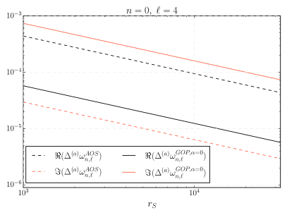
Figure 1: In this plot we show the deviation of the real (black) and imaginary (red) parts of the quasinormal frequency $n=0$ and $\ell=4$ of AOS (dashed line) and GOP with $\alpha=0$ (solid line) effective geometries with respect to general relativity. For this frequency our numerical methods give good enough accuracy. We do not show the GOP prescription with $\alpha=1$ since it gives qualitatively similar results than GOP one with $\alpha=0$.

III.2 Polar perturbations

For polar perturbations, the potential has a more complicated expression than the axial ones. It takes the form

$$\begin{split}{}^{(p)}V_{\ell}(r)&=\frac{G(r)(\ell-1)^{2}(\ell+2)^{2}}{\lambda_{\ell}(r)^{2}}\left[\frac{(\ell-1)(\ell+2)+2}{H(r)}+R(r)\right.\\ &+\left.\frac{H(r)R(r)^{2}}{(\ell-1)^{2}(\ell+2)^{2}}\left((\ell-1)(\ell+2)+\frac{H(r)R(r)}{3}\right)\right],\end{split}$$ (14)

where $R(r)$ is again given by (III.1) and $\lambda_{\ell}(r)$ by

$$\lambda_{\ell}(r)=(\ell-1)(\ell+2)+H(r)R(r).$$ (15)

One can see that the expression above agrees with the one obtained by 2p2 (but it disagrees with the potential of polar perturbations derived in polar-lqc ). By direct inspection, one can also check that it reduces to the standard one in the case of the Schwarzschild classical geometry given by

$$\begin{split}{}^{(p)}V^{GR}_{\ell}(r)&=\left(1-\frac{2Gm}{r}\right)\bigg{[}\frac{\ell(\ell+1)}{r^{2}}\\ &-\frac{6Gm}{r^{3}}\frac{r^{2}\Lambda_{\ell}(\Lambda_{\ell}+2)+3Gm(r-Gm)}{(r\Lambda_{\ell}+3Gm)^{2}}\bigg{]},\end{split}$$ (16)

with $\Lambda_{\ell}=(\ell-1)(\ell+2)/2$. In Table 2 we provide a few dimensionless quasinormal frequencies for polar perturbations of GR, AOS and GOP metrics. We denote them by ${}^{(p)}\omega_{n,\ell}$. We adopt the same choice of parameters than for quasinormal frequencies of axial perturbations, namely, a Schwarzschild radius $r_{S}=10^{3}\,\ell_{P}$ and the two GOP prescriptions ($\alpha=0$ and $\alpha=1$). Again, we see quantitative deviations with respect to the Schwarzschild geometry, but they barely exceed one part in one thousand. Their behavior is very similar to the one of axial perturbations shown in Fig. 1. Up to a small percent, their deviation with respect to general relativity is of the same order of magnitude and it decays as $(r_{S}/\ell_{\rm Pl})^{-2/3}$. Again, for the GOP prescriptions, if instead we choose $\delta x=\ell_{\rm Pl}^{2}/(2r_{0})$, quantum corrections decrease as $(r_{S}/\ell_{\rm Pl})^{-4/3}$. We also checked that several overtones and the fundamental mode share all those properties.

Interestingly, our results also allow us to probe the isospectrality of axial and polar quasinormal modes of these effective geometries. Within our accuracy, we see isospectrality of quasinormal frequencies in the Schwarzschild classical metric. This is not surprising, since it is well known that quasinormal frequencies of Schwarzschild classical geometries are isospectral. In our findings, for these classical geometries, any differences between axial and polar modes are always some orders of magnitude below our error estimation. However, this is not the case of the AOS and GOP regular black holes. Here, isospectrality is broken. Although the violation is very weak, even for these microscopic black holes, the lowest multipole $n=0$ and $\ell=2$ shows the strongest deviation from isospectrality, which happens well above our numerical errors. In Fig. 2, as an example, we show the deviation from isospectrality codified in ${}^{(iso)}\Delta\omega_{n,\ell}^{AOS}=\left({}^{(a)}\omega^{AOS}_{n,\ell}-{}^{(p)}\omega^{AOS}_{n,\ell}\right)$, for a given overtone, as a function of the horizon radius of the black holes, and similarly for the GOP ($\alpha=0$) prescription —the GOP one for $\alpha=1$ shows qualitatively similar results. We consider the radius to be in the interval $r_{S}\in[1000\,\ell_{\rm Pl},32000\,\ell_{\rm Pl}]$. We observe that the violation of isospectrality also decreases with the power $(r_{S}/\ell_{\rm Pl})^{-2/3}$. This behavior seems to be universal regardless of the choice of $n$ and $\ell$ within the modes that we have been able to probe. Hence, for macroscopic black holes, isospectrality is expected to be preserved except for very tiny deviations. In the case of the GOP prescriptions, these corrections decrease as $(r_{S}/\ell_{\rm Pl})^{-4/3}$ if one chooses instead $\delta x=\ell_{\rm Pl}^{2}/(2r_{0})$.

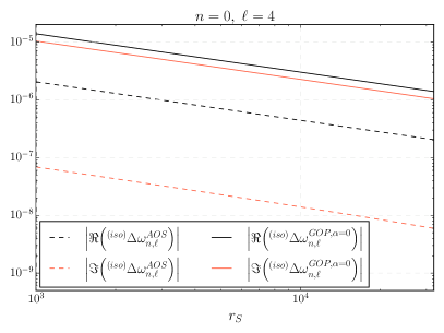
Figure 2: In this plot we show the deviation from isospectrality of the (absolute value of the) real (black) and imaginary (red) parts of the quasinormal frequency $n=0$ and $\ell=4$ of AOS (dashed line) and GOP with $\alpha=0$ (solid line) effective geometries. Our numerical methods give good enough accuracy for this frequency. The GOP prescription with $\alpha=1$ gives qualitatively similar results than $\alpha=0$. Hence, we do not show it here.

IV Conclusions

In this manuscript we study the quasinormal frequencies of axial and polar perturbations of several black hole effective geometries in loop quantum gravity. Concretely, we consider the AOS prescription proposed in aos , as well as the GOP prescriptions derived in gop-imp1 ; gop-imp2 . The effective spacetime line elements are characterized by the functions given in (2) and (4), respectively. We compare them with the Schwarzschild classical space-time. We provide expressions for the effective potential of the radial equations of axial and polar modes valid for general spherically symmetric geometries. Moreover, we complement our study with a similar calculation of scalar and vector perturbations in Appendix A.

In order to compute the quasinormal frequencies, we adopt a high-order WKB approach supplemented with Padé approximants that allow us to increase considerably the accuracy of our calculations. We compare classical and quantum corrected black holes with the same black hole horizon radius. On the one hand, the difference of the quasinormal frequencies between the classical and effective geometries decays always for AOS and GOP prescriptions as $(r_{S}/\ell_{\rm Pl})^{-2/3}$ if, for the latter, one chooses the quantum parameter $\delta x=r_{0}$ in the GOP prescriptions. However, for the GOP one, these quantum corrections decay as $(r_{S}/\ell_{\rm Pl})^{-4/3}$ if one chooses $\delta x=\ell_{\rm Pl}^{2}/(2r_{0})$. Besides, we have also demonstrated numerically that these effective geometries break isopectrality. Namely, quasinormal frequencies of axial and polar perturbations disagree, unlike in the classical theory. However, this violation also dilutes with the radius (i.e. ADM mass) of the black hole as $(r_{S}/\ell_{\rm Pl})^{-2/3}$ (for AOS and GOP prescriptions if $\delta x=r_{0}$), or as $(r_{S}/\ell_{\rm Pl})^{-4/3}$ (for the GOP prescriptions if $\delta x=\ell_{\rm Pl}^{2}/(2r_{0})$). Hence, one should expect large deviations only for microscopic black holes. Nevertheless for macroscopic black holes, our study shows that they are negligible.

It is worth mentioning that we adopt an effective approach that assumes a continuous background geometry and also a particular choice for the effective potentials of the radial equations of axial and polar perturbations that ignores quantum fluctuations of the geometries and couplings originated from other quantum corrections. We must note that GOP effective geometries were derived from a quantum theory, for a particular family of semiclassical states. For instance, they neglect superpositions in the mass and the basis of spin networks. These superpositions will add additional corrections on these effective geometries that are worth to be explored in the future. Besides, these potentials actually suffer from regularization and quantization ambiguities. Despite all that, we expect that our results are robust regarding the breaking of isospectrality, which is the main result of this manuscript. Besides, although we have considered just a few effective geometries, we expect that isospectrality will also be broken in other black hole models kswe-imp ; achou ; gssw ; bmm ; abv ; qmm .

Appendix A quasinormal modes of scalar and vector perturbations

In this Appendix we also compute the quasinormal frequencies of scalar and vector (electromagnetic) perturbations. We follow the same methodology adopted for the axial and polar modes. Expressions for the corresponding potentials can be derived straightforwardly (see for instance aagls ).

The effective potential for scalar (massless) perturbations can be obtained in terms of the metric components as:

$${}^{(s)}V_{\ell}(r)=G(r)\left[\frac{\ell(\ell+1)-2}{H(r)}+\frac{[H^{\prime}(r)]^{2}}{2F(r)H^{2}(r)}+R(r)\right],$$ (17)

where we must recall that the primes denote derivatives with respect to $r$. For the classical Schwarzschild solution, one obtains

$${}^{(s)}V^{GR}_{\ell}(r)=\left(1-\frac{2Gm}{r}\right)\left[\frac{\ell(\ell+1)}{r^{2}}+\frac{2Gm}{r^{3}}\right].$$ (18)

For vector (massless) perturbations the potential takes a simple form:

$${}^{(v)}V_{\ell}(r)=G(r)\,\frac{\ell(\ell+1)}{H(r)}.$$ (19)

This expression reduces to

$${}^{(v)}V^{GR}_{\ell}(r)=\left(1-\frac{2Gm}{r}\right)\frac{\ell(\ell+1)}{r^{2}},$$ (20)

for the classical Schwarzschild geometry.

In Table 3 and Table 4 we show some quasinormal frequencies for the scalar ${}^{(s)}\omega_{n,\ell}$ and vector ${}^{(v)}\omega_{n,\ell}$ perturbations of GR, AOS and GOP metrics. Again, we have considered black holes with horizon radius equal or close to $r_{S}=10^{3}\,\ell_{P}$. As in the axial and polar cases, the deviations from GR are small, but still the accuracy of our method is good enough to show this corrections. In Fig. 3 we see that the differences $\Delta{}^{(v)}\omega_{n,\ell}^{AOS}=({}^{(v)}\omega^{GR}_{n,\ell}-{}^{(v)}\omega^{AOS}_{n,\ell})$ and $\Delta{}^{(v)}\omega_{n,\ell}^{GOP,\alpha=0}=({}^{(v)}\omega^{GR}_{n,\ell}-{}^{(v)}\omega^{GOP,\alpha=0}_{n,\ell})$, for vector perturbations, and $\Delta{}^{(s)}\omega_{n,\ell}^{AOS}=({}^{(s)}\omega^{GR}_{n,\ell}-{}^{(s)}\omega^{AOS}_{n,\ell})$ and $\Delta{}^{(s)}\omega_{n,\ell}^{GOP,\alpha=0}=({}^{(s)}\omega^{GR}_{n,\ell}-{}^{(s)}\omega^{GOP,\alpha=0}_{n,\ell})$, for scalar perturbations, weaken with the mass of the black holes as $(r_{S}/\ell_{\rm Pl})^{-2/3}$.

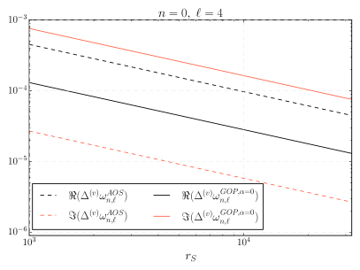
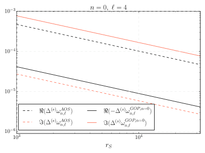
Figure 3: In this plot we show the deviation of the real (black) and imaginary (red) parts of the quasinormal frequency $n=0$ and $\ell=4$ of AOS (dashed line) and GOP with $\alpha=0$ (solid line) effective geometries with respect to general relativity. In the upper panel we show this difference for vector perturbations. In the lower panel for scalar perturbations. In both cases, our computations give good enough accuracy for this frequency. We do not show the GOP prescription with $\alpha=1$ since it gives qualitatively similar results than GOP one with $\alpha=0$.

Appendix B Padé approximants and accuracy of the WKB method

In order to increase the accuracy of the WKB method it is possible to make use of the Padé approximants. Let us summarize the procedure (for details see wkbpade ; konoplyapade ). Here, one starts with the polynomial

$$P_{k}(\xi)=V_{\ell}(r_{0})-\sqrt{-2V_{\ell}^{{}^{\prime\prime}}(r_{0})}\left[\xi\left(n+\frac{1}{2}\right)+\sum_{n=2}^{N}\xi^{n}\Lambda_{n}\right],$$ (21)

from the formula (10) where the parameter $\xi$ is introduced to allow us to keep track of the order of the polynomial, so that $\tilde{\omega}_{n,\ell}^{2}=P_{k}(1)$, where $k$ is the WKB order. Then, we approximate $P_{k}(\xi)$ around $\xi=0$ with the family of the Padé approximants

$$P_{\tilde{n}/\tilde{m}}(\xi)=\frac{Q_{0}+Q_{1}\,\xi+...+Q_{\tilde{n}}\,\xi^{\tilde{n}}}{R_{0}+R_{1}\,\xi+...+R_{\tilde{m}}\,\xi^{\tilde{m}}},$$ (22)

where $\tilde{n}+\tilde{m}=k$ and $Q_{i},R_{i}$ are determined such that

$$P_{\tilde{n}/\tilde{m}}(\xi)-P_{k}(\xi)=\mathcal{O}(\xi^{k+1}).$$ (23)

Once an approximation $P_{\tilde{n}/\tilde{m}}(\xi)$ has been chosen, to compute the quasinormal frequencies, one takes $\tilde{\omega}_{n}^{2}=P_{\tilde{n}/\tilde{m}}(1)$. For example, at first order, the WKB formula admits two expressions

$$\begin{split}\tilde{\omega}_{n}^{2}&=P_{1/0}(1)=P_{1}(1)=V_{\ell}(r_{0})-\sqrt{-V^{\prime\prime}_{\ell}(r_{0})}\left(n+\frac{1}{2}\right),\\ \tilde{\omega}_{n}^{2}&=P_{0/1}(1)=\frac{V_{\ell}(r_{0})}{V_{\ell}(r_{0})-\sqrt{-V_{\ell}^{\prime\prime}(r_{0})}\left(n+\frac{1}{2}\right)}.\end{split}$$ (24)

For higher orders, it has been observed wkbpade ; konoplyapade that the Padé approximants $P_{\tilde{n}/\tilde{m}}$ with $\tilde{n}\approx\tilde{m}$ usually give better results than the standard WKB formula $P_{\tilde{m}/0}$. Also, as the WKB order increases, all the alternative approximations give similar results.

We use code to compute the quasinormal frequencies together with an estimation of their error. The procedure is as follows. If we consider, for instance, the 10th WKB order, there are 11 Padé approximants ($P_{0/10}$, $P_{1/9}$, …, $P_{10/0}$). The criterion we adopt to select the most accurate approximants is the same as in konoplyapade . Here, one computes all the mean values of two closest frequencies

$$\bar{\omega}_{\tilde{n}/\tilde{m}}^{(p)}=\frac{\tilde{\omega}_{(\tilde{n}+p)/(\tilde{m}-p)}+\tilde{\omega}_{\tilde{n}/\tilde{m}}}{2},$$ (25)

for $p$ a given set of integers that will be selected by the WKB approximation. For instance, for the 10th WKB order $p=1,\ldots,4$. Then for each value of $p$, we select the two estimations $\bar{\omega}_{\tilde{n}/\tilde{m}}^{(p)}$ for which the relative difference between the corresponding Padé approximants (or frequencies) is minimum. Eventually, the final quasinormal frequency is the mean of these eight Padé approximants and its absolute error given by the standard deviation of this set of estimations. We denote them by $\sigma_{axial}$ and $\sigma_{polar}$ for the axial and polar quasinormal frequencies, respectively. The code code follows this criterion, providing mean values and errors (see konoplyapade for details) as we just explained.

The estimations of the errors given in Table 5 are calculated in the following way: given $\sigma_{axial}$ and $\sigma_{polar}$, we define the total error as

$$\sigma=\sqrt{\sigma_{axial}^{2}+\sigma_{polar}^{2}}.$$ (26)

We then compute the percentage relative error over the absolute value of the mean between the axial and polar quasinormal frequencies.

Appendix C Tables

In this appendix we provide numerical values of some of the dimensionless quasinormal frequencies, namely, we show $\omega_{n,\ell}=(r_{S}/2G)\,\tilde{\omega}_{n,\ell}$, as is customary in the literature.

Axial Perturbations
($n$,$\ell$)	Schwarzschild	AOS ($r_{S}=10^{3}\,\ell_{P}$)
(0,2)	0.74733225 - 0.17792806$i$	0.74771876 - 0.17787563$i$
(1,2)	0.69322645 - 0.54811740$i$	0.69360839 - 0.54794196$i$
(0,3)	1.19888658 - 0.18540612$i$	1.19942465 - 0.18535672$i$
(1,3)	1.16528891 - 0.56259764$i$	1.16581711 - 0.56244359$i$
(0,4)	1.61835676 - 0.18832792$i$	1.61905472 - 0.18828092$i$
(1,4)	1.59326305 - 0.56866870$i$	1.59395164 - 0.56852466$i$
(0,5)	2.02459062 - 0.18974103$i$	2.02544902 - 0.18969535$i$
(1,5)	2.00444206 - 0.57163476$i$	2.00529218 - 0.57149586$i$
(0,6)	2.42401964 - 0.19053169$i$	2.42503820 - 0.19048680$i$
(1,6)	2.40714795 - 0.57329985$i$	2.40815924 - 0.57316390$i$
	GOP ($\alpha=0$, $r_{S}=10^{3}\,\ell_{P}$)	GOP ($\alpha=1$, $r_{S}=10^{3}\,\ell_{P}$)
(0,2)	0.74736483 - 0.17720680$i$	0.74736491 - 0.17720674$i$
(1,2)	0.69401982 - 0.54578773$i$	0.69401995 - 0.54578751$i$
(0,3)	1.19894618 - 0.18468114$i$	1.19894629 - 0.18468108$i$
(1,3)	1.16577313 - 0.56034440$i$	1.16577326 - 0.56034419$i$
(0,4)	1.61841428 - 0.18758921$i$	1.61841442 - 0.18758914$i$
(1,4)	1.59363598 - 0.56640627$i$	1.59363614 - 0.56640607$i$
(0,5)	2.02464204 - 0.18899367$i$	2.02464221 - 0.18899361$i$
(1,5)	2.00474707 - 0.56936206$i$	2.00474725 - 0.56936186$i$
(0,6)	2.42406539 - 0.18977889$i$	2.42406539 - 0.18977889$i$
(1,6)	2.40740646 - 0.57101967$i$	2.40740646 - 0.57101967$i$

Table 1: Quasinormal frequencies for the first overtones of the axial perturbations.

Polar Perturbations
($n$,$\ell$)	Schwarzschild	AOS ($r_{S}=10^{3}\,\ell_{P}$)
(0,2)	0.74734291 - 0.17792545$i$	0.74770137 - 0.17786831$i$
(1,2)	0.69337238 - 0.54785794$i$	0.69371455 - 0.54766125$i$
(0,3)	1.19888656 - 0.18540609$i$	1.19941686 - 0.18535615$i$
(1,3)	1.16528740 - 0.56259608$i$	1.16580600 - 0.56243957$i$
(0,4)	1.61835675 - 0.18832792$i$	1.61905147 - 0.18828080$i$
(1,4)	1.59326306 - 0.56866870$i$	1.59394788 - 0.56852416$i$
(0,5)	2.02459062 - 0.18974103$i$	2.02544735 - 0.18969532$i$
(1,5)	2.00444206 - 0.57163476$i$	2.00529032 - 0.57149572$i$
(0,6)	2.42401964 - 0.19053169$i$	2.42503722 - 0.19048679$i$
(1,6)	2.40714795 - 0.57329985$i$	2.40815818 - 0.57316385$i$
	GOP ($\alpha=0$, $r_{S}=10^{3}\,\ell_{P}$)	GOP ($\alpha=1$, $r_{S}=10^{3}\,\ell_{P}$)
(0,2)	0.74749081 - 0.17733983$i$	0.74749089 - 0.17733977$i$
(1,2)	0.69407330 - 0.54597173$i$	0.69407343 - 0.54597152$i$
(0,3)	1.19897954 - 0.18471131$i$	1.19897964 - 0.18471125$i$
(1,3)	1.16577795 - 0.56043389$i$	1.16577808 - 0.56043369$i$
(0,4)	1.61842820 - 0.18759958$i$	1.61842834 - 0.18759952$i$
(1,4)	1.59364290 - 0.56643745$i$	1.59364305 - 0.56643725$i$
(0,5)	2.02464917 - 0.18899817$i$	2.02464934 - 0.18899811$i$
(1,5)	2.00475176 - 0.56937559$i$	2.00475194 - 0.56937540$i$
(0,6)	2.42406933 - 0.18978122$i$	2.42406953 - 0.18978115$i$
(1,6)	2.40740936 - 0.57102668$i$	2.40740957 - 0.57102648$i$

Table 2: Quasinormal frequencies for the first overtones of the polar perturbations.

Scalar Perturbations
($n$,$\ell$)	Schwarzschild	AOS ($r_{S}=10^{3}\,\ell_{P}$)
(0,0)	0.22106137 - 0.20937335$i$	0.22140540 - 0.20925624$i$
(1,0)	0.18850053 - 0.70053554$i$	0.18859010 - 0.70054267$i$
(0,1)	0.58587217 - 0.19532140$i$	0.58621916 - 0.19527153$i$
(1,1)	0.52916747 - 0.61270000$i$	0.52946242 - 0.61254038$i$
(0,2)	0.96728773 - 0.19351755$i$	0.96775106 - 0.19347264$i$
(1,2)	0.92770066 - 0.59120829$i$	0.92813871 - 0.59106793$i$
(0,3)	1.35073247 - 0.19299926$i$	1.35133550 - 0.19295544$i$
(1,3)	1.32134299 - 0.58456958$i$	1.32192959 - 0.58443479$i$
(0,4)	1.73483128 - 0.19278338$i$	1.73558221 - 0.19273997$i$
(1,4)	1.71161607 - 0.58175204$i$	1.71235477 - 0.58161967$i$
	GOP ($\alpha=0$, $r_{S}=10^{3}\,\ell_{P}$)	GOP ($\alpha=1$, $r_{S}=10^{3}\,\ell_{P}$)
(0,0)	0.22065868 - 0.20832678$i$	0.22065871 - 0.20832671$i$
(1,0)	0.18841088 - 0.69652318$i$	0.18841087 - 0.69652280$i$
(0,1)	0.58574403 - 0.19449923$i$	0.58574409 - 0.19449915$i$
(1,1)	0.52965894 - 0.60989852$i$	0.52965911 - 0.60989817$i$
(0,2)	0.96721207 - 0.19273001$i$	0.96721215 - 0.19272994$i$
(1,2)	0.92812583 - 0.58870416$i$	0.92812594 - 0.58870394$i$
(0,3)	1.35067881 - 0.19222161$i$	1.35067892 - 0.19222154$i$
(1,3)	1.32166241 - 0.58216341$i$	1.32166254 - 0.58216321$i$
(0,4)	1.73478970 - 0.19200982$i$	1.73478985 - 0.19200976$i$
(1,4)	1.71186939 - 0.57938690$i$	1.71186954 - 0.57938670$i$

Table 3: Quasinormal frequencies for the first overtones of the scalar perturbations.

Vector Perturbations
($n$,$\ell$)	Schwarzschild	AOS ($r_{S}=10^{3}\,\ell_{P}$)
(0,1)	0.49652620 - 0.18497687$i$	0.49677857 - 0.18493659$i$
(1,1)	0.42896489 - 0.58735295$i$	0.42917124 - 0.58722013$i$
(0,2)	0.91519104 - 0.19000886$i$	0.91559456 - 0.18996650$i$
(1,2)	0.87308476 - 0.58142022$i$	0.87346490 - 0.58128680$i$
(0,3)	1.31379734 - 0.19123244$i$	1.31435699 - 0.19118977$i$
(1,3)	1.28347488 - 0.57945680$i$	1.28401884 - 0.57932526$i$
(0,4)	1.70619039 - 0.19171987$i$	1.70690733 - 0.19167710$i$
(1,4)	1.68253412 - 0.57862935$i$	1.68323922 - 0.57849884$i$
(0,5)	2.09582556 - 0.19196334$i$	2.09670029 - 0.19192054$i$
(1,5)	2.07644178 - 0.57820772$i$	2.07730694 - 0.57807779$i$
	GOP ($\alpha=0$, $r_{S}=10^{3}\,\ell_{P}$)	GOP ($\alpha=1$, $r_{S}=10^{3}\,\ell_{P}$)
(0,1)	0.49512802 - 0.18174827$i$	0.49512801 - 0.18174817$i$
(1,1)	0.42344855 - 0.57974580$i$	0.42344839 - 0.57974555$i$
(0,2)	0.91441759 - 0.18693022$i$	0.91441764 - 0.18693012$i$
(1,2)	0.86956543 - 0.57304523$i$	0.86956536 - 0.57304497$i$
(0,3)	1.31325754 - 0.18818198$i$	1.31325763 - 0.18818188$i$
(1,3)	1.28092560 - 0.57075050$i$	1.28092561 - 0.57075023$i$
(0,4)	1.70577457 - 0.18867960$i$	1.70577469 - 0.18867951$i$
(1,4)	1.68053934 - 0.56977960$i$	1.68053940 - 0.56977932$i$
(0,5)	2.09548701 - 0.18892794$i$	2.09548717 - 0.18892784$i$
(1,5)	2.07480446 - 0.56928366$i$	2.07480456 - 0.56928338$i$

Table 4: Quasinormal frequencies for the first overtones of vector perturbations.

Estimation of the errors (%)
($n$,$\ell$)	Schwarzschild	AOS ($r_{S}=10^{3}\,\ell_{P}$)
(0,2)	8.32073$\times 10^{-4}$	8.28774$\times 10^{-4}$
(1,2)	5.37259$\times 10^{-2}$	5.34523$\times 10^{-2}$
(0,3)	3.78222$\times 10^{-6}$	3.65464$\times 10^{-6}$
(1,3)	2.43954$\times 10^{-5}$	2.47351$\times 10^{-5}$
(0,4)	4.13316$\times 10^{-8}$	4.02860$\times 10^{-8}$
(1,4)	1.06444$\times 10^{-6}$	1.02453$\times 10^{-6}$
(0,5)	1.83706$\times 10^{-9}$	1.65610$\times 10^{-9}$
(1,5)	6.01152$\times 10^{-8}$	5.93357$\times 10^{-8}$
(0,6)	5.17149$\times 10^{-11}$	4.51964$\times 10^{-11}$
(1,6)	8.12115$\times 10^{-9}$	8.06923$\times 10^{-9}$
	GOP ($\alpha=0$, $r_{S}=10^{3}\,\ell_{P}$)	GOP ($\alpha=1$, $r_{S}=10^{3}\,\ell_{P}$)
(0,2)	9.04563$\times 10^{-4}$	9.04640$\times 10^{-4}$
(1,2)	5.08751$\times 10^{-2}$	5.08751$\times 10^{-2}$
(0,3)	2.56594$\times 10^{-6}$	2.56612$\times 10^{-6}$
(1,3)	2.35593$\times 10^{-5}$	2.35524$\times 10^{-5}$
(0,4)	2.26845$\times 10^{-8}$	2.26960$\times 10^{-8}$
(1,4)	6.71517$\times 10^{-7}$	6.70473$\times 10^{-7}$
(0,5)	5.11426$\times 10^{-10}$	5.09071$\times 10^{-10}$
(1,5)	5.05602$\times 10^{-8}$	5.04985$\times 10^{-8}$
(0,6)	2.28438$\times 10^{-11}$	2.31124$\times 10^{-11}$
(1,6)	7.27388$\times 10^{-9}$	7.26642$\times 10^{-9}$

Table 5: Estimations of the errors using the 10th WKB order with Padé approximants.

References

- (1) M. Isi, M. Giesler, W. M. Farr, M. A. Scheel and S. A. Teukolsky, “Testing the no-hair theorem with GW150914,” Phys. Rev. Lett. 123, 111102 (2019).
- (2) T. Regge and J. A. Wheeler, “Stability of a Schwarzschild singularity,” Phys. Rev. 108, 1063-1069 (1957).
- (3) F. J. Zerilli, “Effective potential for even parity Regge-Wheeler gravitational perturbation equations,” Phys. Rev. Lett. 24, 737-738 (1970).
- (4) S. Chandrasekhar and S. L. Detweiler, “The quasi-normal modes of the Schwarzschild black hole,” Proc. Roy. Soc. Lond. A 344, 441-452 (1975).
- (5) F. Moulin and A. Barrau, “Analytical proof of the isospectrality of quasinormal modes for Schwarzschild-de Sitter and Schwarzschild-Anti de Sitter spacetimes,” Gen. Rel. Grav. 52, 82 (2020).
- (6) M. Lenzi and C. F. Sopuerta, “Darboux Covariance: A Hidden Symmetry of Perturbed Schwarzschild Black Holes,” , Phys. Rev. D 104, 124068 (2021)..
- (7) C.B. Prasobh and V.C. Kuriakose, “Quasinormal Modes of Lovelock Black Holes,” Eur. Phys. J. C 74, 3136 (2014).
- (8) S. Bhattacharyya and S. Shankaranarayanan, “Distinguishing general relativity from Chern-Simons gravity using gravitational wave polarizations,” Phys. Rev. D 100, 024022 (2019).
- (9) C. Chen and S. Park, “Black hole quasinormal modes and isospectrality in Deser-Woodard nonlocal gravity,” Phys. Rev. D 103, 064029 (2021).
- (10) V. Cardoso,M. Kimura, A. Maselli, E. Berti, C. F. B. Macedo and R. McManus, “Parametrized black hole quasinormal ringdown: Decoupled equations for nonrotating black holes,” Phys. Rev. D 99, 104077 (2019).
- (11) R. McManus, E. Berti, C. F. B. Macedo, M. Kimura, A. Maselli and V. Cardoso, “Parametrized black hole quasinormal ringdown. II. Coupled equations and quadratic corrections for nonrotating black holes,” Phys. Rev. D 100, 044061 (2019).
- (12) M. B. Cruz, F. A. Brito and C. A. S. Silva, “Polar gravitational perturbations and quasinormal modes of a loop quantum gravity black hole,” Phys. Rev. D 102, 044063 (2020).
- (13) A. Ashtekar and P. Singh, “Loop Quantum Cosmology: A Status Report,” Class. Quant. Grav. 28, 213001 (2011).
- (14) M. Bouhmadi-López, S. Brahma, C. Y. Chen, P. Chen and D. Yeom, “A consistent model of non-singular Schwarzschild black hole in loop quantum gravity and its quasinormal modes,” JCAP 07, 066 (2020).
- (15) R. G. Daghigh, M. D. Green and G. Kunstatter, “Scalar Perturbations and Stability of a Loop Quantum Corrected Kruskal Black Hole,” Phys. Rev. D 103, 084031 (2021).
- (16) Y. C. Liu, J. X. Feng, F. W. Shu, A. Wang, “Extended geometry of Gambini-Olmedo-Pullin polymer black hole and its quasinormal spectrum,” Phys. Rev. D 104, 106001 (2021).
- (17) J. L. Jaramillo, R. Panosso Macedo, L. A. Sheikh, “Pseudospectrum and black hole quasi-normal mode (in)stability,” Phys. Rev. X 11, 031003 (2021); “Gravitational wave signatures of black hole quasi-normal mode instability,” arXiv:2105.03451 (2021).
- (18) M. H. Y. Cheung, K. Destounis, R. Panosso Macedo, E. Berti, V. Cardoso, “The elephant and the flea: destabilizing the fundamental mode of black holes,” arXiv:2111.05415 (2021).
- (19) M. Maggiore, “Physical Interpretation of the Spectrum of Black Hole Quasinormal Modes,” Phys. Rev. Lett. 100, 141301 (2008).
- (20) I. Agullo, V. Cardoso, A. del Rio, M. Maggiore, J. Pullin, “Potential gravitational-wave signatures of quantum gravity,” Phys. Rev. Lett. 126, 041302 (2021).
- (21) S. Carneiro and C. Pigozzo, “Quasinormal modes and horizon area quantisation in Loop Quantum Gravity,” Gen. Relat. Gravit. 54, 20 (2022).
- (22) A. Ashtekar, J. Olmedo and P. Singh, “Quantum Transfiguration of Kruskal Black Holes,” Phys. Rev. Lett. 121, 241301 (2018); “Quantum extension of the Kruskal spacetime,” Phys. Rev. D 98, 126003 (2018).
- (23) A. Ashtekar and J. Olmedo, “Properties of a recent quantum extension of the Kruskal geometry,” Int. J. Mod. Phys. D 29, 2050076 (2020).
- (24) R. Gambini, J. Olmedo and J. Pullin, “Spherically symmetric loop quantum gravity: analysis of improved dynamics,” Class. Quant. Grav. 37, 205012 (2020).
- (25) R. Gambini, J. Olmedo and J. Pullin, “Loop Quantum Black Hole Extensions Within the Improved Dynamics,” Front. Astron. Space Sci. 8, 74 (2021).
- (26) I. Agullo, J. Barbero G., J. Diaz-Polo, E. Fernandez-Borja, and E. J. Villasenor, “Black hole state counting in LQG: A Number theoretical approach,” Phys. Rev. Lett. 100 211301 (2008).
- (27) I. Agullo, J. Fernando Barbero, E. F. Borja, J. Diaz-Polo, and E. J. Villasenor, “Detailed black hole state counting in loop quantum gravity,” Phys. Rev. D 82, 084029 (2010).
- (28) A. Barrau, X. Cao, K. Noui, A. Perez, “Black hole spectroscopy from Loop Quantum Gravity models,” Phys. Rev. D 92, 124046 (2015).
- (29) R. Gambini and J. Pullin, “Loop quantization of the Schwarzschild black hole,” Phys. Rev. Lett. 110, 211301 (2013).
- (30) R. Gambini, J. Olmedo and J. Pullin, “Quantum black holes in Loop Quantum Gravity,” Class. Quant. Grav. 31, 095009 (2014).
- (31) J. Olmedo, “Brief review on black hole loop quantization,” Universe 2, 12 (2016).
- (32) J. G. Kelly, R. Santacruz and E. Wilson-Ewing, “Effective loop quantum gravity framework for vacuum spherically symmetric spacetimes,” Phys. Rev. D 102, 106024 (2020).
- (33) V. Moncrief, “Gravitational perturbations of spherically symmetric systems. I. The exterior problem,” Ann. Phys. 88, 323 (1974).
- (34) D. Brizuela and J. M. Martin-Garcia, “Hamiltonian theory for the axial perturbations of a dynamical spherical background,” Class. Quant. Grav. 26, 015003 (2009).
- (35) D. Brizuela, “A generalization of the Zerilli master variable for a dynamical spherical spacetime,” Class. Quant. Grav. 32, 135005 (2015).
- (36) U. H. Gerlach and U.K. Sengupta “Gauge-invariant perturbations on most general spherically symmetric space-times,” Phys. Rev. D 19, 2268-2272 (1979).
- (37) O. Sarbach and M. Tiglio, “Gauge-invariant perturbations of Schwarzschild black holes in horizon-penetrating coordinates,” Phys. Rev. D 64, 084016 (2001).
- (38) K. Martel and E. Poisson, “Gravitational perturbations of the Schwarzschild spacetime: A practical covariant and gauge-invariant formalism,” Phys. Rev. D 71, 104003 (2005).
- (39) J. L. Ripley and K. Yagi, “Black hole perturbation under a 2 + 2 decomposition in the action,” Phys. Rev. D 97, 024009 (2018).
- (40) S. Iyer and C. M. Will,“Black Hole Normal Modes: A WKB Approach. 1. Foundations and Application of a Higher Order WKB Analysis of Potential Barrier Scattering,” Phys. Rev. D 35, 3621 (1987).
- (41) R. A. Konoplya, “Quasinormal behavior of the d-dimensional Schwarzschild black hole and higher order WKB approach,” Phys. Rev. D 68, 024018 (2003).
- (42) The Mathematica package with the WKB formula of 13th order and Padé approximations ready for calculation of the quasinormal modes and grey-body factors, as well as examples of such calculations for the Schwarzschild black hole are publicly available to download from https://goo.gl/nykYGL .
- (43) Y. C. Liu, J. X. Feng, F. W. Shu and A. Wang, “Extended geometry of Gambini-Olmedo-Pullin polymer black hole and its quasinormal spectrum,” Phys. Rev. D 104, no.10, 106001 (2021).
- (44) J. Ben Achour, F. Lamy, H. Liu, and K. Noui, “Polymer Schwarzschild black hole: An effective metric,” EPL 123, 20006 (2018).
- (45) W. C. Gan, N. O. Santos, F. W. Shu and A. Wang, “Properties of the spherically symmetric polymer black holes,” Phys. Rev. D 102, 124030 (2020).
- (46) N. Bodendorfer, F. M. Mele, and J. Münch, “(b,v)-type variables for black to white hole transitions in effective loop quantum gravity,” Phys. Lett. B 819, 136390 (2021).
- (47) A. Alonso-Bardaji, D. Brizuela, and R. Vera, “An effective model for the quantum Schwarzschild black hole,” arxiv: 2112.12110 [gr-qc].
- (48) A. García-Quismondo, and G. A. Mena Marugán, “Exploring alternatives to the Hamiltonian calculation of the Ashtekar-Olmedo-Singh black hole solution,” Front. Astron. Space Sci 8, 701723 (2021).
- (49) A. Arbey, J. Auffinger, M. Geiller, E. R. Livine, and F. Sartini, “Hawking radiation by spherically-symmetric static black holes for all spins: Teukolsky equations and potentials,” Phys. Rev. D 103, 104010 (2021).
- (50) J. Matyjasek and M. Opala, “Quasinormal modes of black holes. The improved semianalytic approach,” Phys. Rev. D 96, no.2, 024011 (2017).
- (51) R. A. Konoplya, A. Zhidenko and A. F. Zinhailo, “Higher order WKB formula for quasinormal modes and grey-body factors: recipes for quick and accurate calculations,” Class. Quant. Grav. 36, 155002 (2019).