Lévy processes in bounded domains: Path-wise reflection scenarios and signatures of confinement.

Abstract

We discuss an impact of various (path-wise) reflection-from-the barrier scenarios upon confining properties of a paradigmatic family of symmetric $\alpha$-stable Lévy processes, whose permanent residence in a finite interval on a line is secured by a two-sided reflection. Depending on the specific reflection ”mechanism”, the inferred jump-type processes differ in their spectral and statistical characteristics, like e.g. relaxation properties, and functional shapes of invariant (equilibrium, or asymptotic near-equilibrium) probability density functions in the interval. The analysis is carried out in conjunction with attempts to give meaning to the notion of a reflecting Lévy process, in terms of the domain of its motion generator, to which an invariant pdf (actually an eigenfunction) does belong.

I Motivation

We consider symmetric Lévy jump-type stochastic processes, which are confined in an interval $[0,b]\subset R,b>0$, with reflecting endpoints (a concept hampered by ambiguities, to be resolved in below). The corresponding random dynamics, usually is formalized in terms of stochastic differential equations with reflecting boundary conditions (their meaning needs to be specified with due care). The inferred time evolution of associated probability density functions (always defined on the whole of $R$, albeit with exterior restrictions in $R\setminus(0,b)$), in the large time asymptotic is expected to show symptoms of convergence to an equilibrium pdf (stationary or steady state function), which needs to belong to the domain of the properly ”tailored” fractional Laplacian, c.f. [1, 2, 3]. The latter is regarded as the random motion generator of the reflected Lévy process.

As discussed in [1], the assignment of a proper motion generator to the Lévy jump-type stochastic process in a bounded domain (any sort, there are many options) is not at all obvious, and path-wise reflecting boundary data need to be confronted and reconciled with a variety of admissible boundary data for the nonlocally defined fractional Laplacian. These include both spatial domain restrictions and boundary constraints of the Dirichlet and Neumann-type, which define the admissible function space.

Here we encounter a number of problems: (i) there is no unique definition of the boundary-data-respecting fractional Laplacian in the interval, (ii) there is no unique technical implementation of the Neumann-type reflecting boundary condition, (iii) a particular path-wise procedure, telling how a reflection is executed at the barrier (e.g. detailed reflecting boundary conditions for the stochastic process) appears not to be an innocent choice, and may have a serious impact on the functional shape of asymptotic probability densities (we shall pay some attention to this point in below), (iv) for each reflection-at-the-barrier scenario, an assignment of the proper motion generator needs to be enabled, and in reverse; albeit there is no one-to-one correspondence.

We anticipate the outcome of our subsequent discussion, by emphasizing the impact of the physics-oriented reasoning in the study of random motion and Lévy processes in particular. In case of bounded domains, the choice of the reflection-at-the boundary ”mechanism” appears to be a major discrimination tool between different options for what is to be consistently named a reflected Lévy process.

The term ”fractional Laplacian” refers to the nonlocally defined operator $(-\Delta)^{\alpha/2}$, which is interpreted as the generator of a symmetric $\alpha$-stable Lévy process on $R$, [1]. Its ”tailoring” refers to a profound problem of deducing the appropriate reflection-restricted form $(-\Delta)^{\alpha/2}\rightarrow(-\Delta)^{\alpha/2}_{\cal{R}}$, where the subscript $\cal{R}$ indicates that suitable boundary conditions are imposed upon $(-\Delta)^{\alpha/2}$. This includes both spatial domain restrictions and operator domain restrictions in the form of functional constraints of the Neumann-type, see [1] and a subsequent discussion in Section V.

It is clear that the prescribed path-wise reflection scenario for the jump-type process is encoded in the inferred fractional differential equation $\partial_{t}\rho(x,t)=-(-\Delta)^{\alpha/2}_{\cal{R}}\rho(x,t)$, governing the time evolution of probability density functions and setting their asymptotic. Different reflection recipes may result in inequivalent invariant pdfs. This we shall demonstrate in below.

For comparison we recall the Brownian form $\partial_{t}\rho=\Delta\rho$, and recall that the ordinary Laplacian is negative-definite. We mention that the standard reflected Brownian motion is understood as a Wiener process in an interval with reflecting boundaries. The casual Neumann condition, which specifies values of the derivative of the stationary pdf at the boundaries, is fully compatible with the path-wise instantaneous reflection scenario. On formal grounds the Brownian reflection mechanism refers to so-called reflection principle, which is known not to be valid for Lévy processes. That, in view of the nonlocality of fractional Laplacians and discontinuities of jump-type sample paths. Accordingly, the terms ”suitable”, ”appropriate” and ”reflecting” become ambiguous in the Lévy processes context.

In the mathematical literature one encounters attempts to define reflected Lévy processes by means of Neumann-type constraints (like e.g. local and nonlocal notions of the ”normal derivative”) imposed on the spatially constrained fractional Laplacian, [13]-[19]. There is no general consensus concerning the proper generalisation of the Neumann condition from the Brownian to the (reflecting) Lévy framework. The pertinent Neumann-type conditions happen to be inequivalent, refer to (induce, or alternatively - result from) inequivalent path-wise reflection scenarios, and might imply incompatible profiles of the inferred stationary pdfs. This in turn needs to be reconciled with the inherent nonlocality of the fractional Laplacian $(-\Delta)^{\alpha/2}$, which gives rise to its varied, inequivalent domain-restricted versions, [1, 4, 5, 6].

Let us mention that in Ref. [1], in the general discussion of Lévy processes in bounded domains, a rough distinction between the Dirichlet and Neumann boundary data has been encoded in the notation $(-\Delta)^{\alpha/2}_{\cal{D}}$ and $(-\Delta)^{\alpha/2}_{\cal{N}}$ respectively.

Our notation $(-\Delta)^{\alpha/2}_{\cal{R}}$, refers to an anticipated existence of the family of inequivalent ”reflecting processes” in the interval, with motion generators subject to inequivalent (albeit semantically ”reflecting”) constraints, which we loosely abbreviate as Neumann-type boundary data. These in turn rely on the presumed microscopic (path-wise) reflection scenarios in the vicinity of the barrier and/or at the barrier location. Moreover, in principle one may admit random dynamics with forth and back jumps, which overshoot barriers at $0$ and $b$ from the interior of the interval, provided an instantaneous return to $(0,b)$ follows.

Here, it is useful to mention a concept of the return processes, c.f. [39, 40], thoroughly analyzed for the case of Cauchy noise ($\alpha$-stable with $\alpha=1$). Notwithstanding, the instantaneous random return scenario actually appears to underlie the concept of nonlocal Neumann boundary conditions for fractional Laplacians in a bounded domain, as introduced in Refs. [16, 17, 18].

In the above discussion, we have been somewhat freely moving between the path-wise and fractional Laplacian implementations of Lévy processes, although they look disparately diverse. Actually, this is not the case, there is a deep connection between them.

The $\alpha$-stable random variable $X$ (and the corresponding stochastic process $X(t)\equiv X_{t}$) can be introduced by means of its characteristic function $\phi(p)=E[\exp(ipX)]$, which is uniquely related to the corresponding probability density function $\rho(x)$ by the Fourier transform $\rho(x)=(1/2\pi)\int_{R}\phi(p)\exp(-ipx)dp$. (Dimensional constants are scaled away.)

For symmetric Lévy processes on $R$, we adopt the logarithmic parametrization of the characteristic function:

$$\ln\phi(p)=-\sigma^{\alpha}|p|^{\alpha}=-\sigma^{\alpha}F(p)$$ (1)

where $\alpha\in(0,2]$ and $\sigma>0$ is a scale parameter, related to a full width of $\rho(x)$ at its half-maximum (FWHM), [8, 9, 10, 2]. Since $\alpha$-stable pdfs have no finite variance, the familiar notion of a ”standard deviation” is undefined. For the exemplary Cauchy case, $\alpha=1$ in Eq. (1), we have $\rho_{\alpha=1}(x)=\sigma/\pi(x^{2}+\sigma^{2})$ and the FWHM reads $2\sigma$.

The scale factor $\sigma$ can be eliminated from the formalism. Namely, let us assume that the stable random variable $X$ has a probability distribution $\rho(x)$ fixed by (1). We encode this assignment by the notation $X\sim S_{\alpha}(\sigma)$, borrowed from Refs. [8, 10]. Once we have given $X\sim S_{\alpha}(1)$, then for the rescaled random variable $Y=\sigma X$ we have $Y\sim S_{\alpha}(\sigma)$. Thus, for a given stability index $\alpha$, the probability distribution $S_{\alpha}(1)$ actually stands for a reference one. From now on we associate the random variable $X$ exclusively with $S_{\alpha}(1)$, i.e. we presume $X\sim S_{\alpha}(1)$. This allows us to proceed with $E[\exp(ipX]=\exp[-F(p)]$, instead of Eq. (1) proper.

Since any Lévy process has the property that for all $t\geq 0$, there holds

$$E[\exp(ipX_{t})]=\exp[-tF(p)],$$ (2)

and we have uniquely determined the time-dependence $\rho(x)\rightarrow\rho(x,t)$ of the reference pdf, and its $\sigma$-scaled versions. The generator of such dynamics and the related fractional Fokker-Planck equation can be deduced as follows.

The notation $F(p)=|p|^{\alpha}$ of Eq. (1), sets a direct link with the fractional semigroup dynamics, [1, 4, 5]. To this end we invoke a substitution procedure, which actually amounts to a canonical quantization step, [12], (up to the explicit presence of $\hbar$):

$$p\rightarrow\hat{p}=-i\nabla\Longrightarrow F(p)\rightarrow F(\hat{p})=(-\Delta)^{\alpha/2}\,.$$ (3)

Since we refer to the standard Fourier representation, a casual quantum mechanical operator notion $(\hat{x}f)(x)=xf(x)$ is implicit. The inferred semigroup operator $\exp[-tF(\hat{p})$ gives rise to the fractional Fokker-Planck equation (no drifts, the fractional Laplacian is the motion generator)

$$\partial_{t}\rho(x,t)=-(-\Delta)^{\alpha/2}\rho(x,t),$$ (4)

with $\rho_{0}(x)$ given as the initial $t=1$ datum.

To justify the recipe (3) one may invoke the Fourier multiplier representation of the fractional Laplacian, [1]:

$${\cal{F}}[(-\Delta)^{\alpha/2}f](k)=|k|^{\alpha}{\cal{F}}[f](k),$$ (5)

while remembering that it is $-(-\Delta)^{\alpha/2}$, which is a fractional analog of the Laplacian $\Delta$.

We prefer to give meaning to the quantization procedure (3), by employing the Lévy-Khinchine formula for the characteristic exponent $F(p)$ of the $\alpha$-stable random variable. In one spatial dimension, we ultimately deal with a reduced integral expression, (the Cauchy principal value of the integral is implicit):

$${F(p)=-\int_{-\infty}^{+\infty}[exp(ipy)-1]\nu(dy)}$$ (6)

where $\nu(dy)$ stands for the Lévy measure. In view of (3), we have defined the action of the semigroup generator $-F(\hat{p})$ on functions in its domain according to:

$$(-\Delta)^{\alpha/2}f(x)=F(\hat{p})f(x)=-(p.v)\int_{R}[f(x+y)-f(x)]\nu(dy).$$ (7)

We emphasize that a generically singular behavior of the Lévy measure in the vicinity of zero needs the (counter)term containing $-f(x)$ for consistency reasons. In the above formulas, the Lévy measure reads:

$$\nu(dy)={\frac{\mathcal{A}_{\alpha}}{|y|^{1+\alpha}}}\,dy=\left[{\Gamma(1+\alpha)\sin\frac{\pi\alpha}{2}}\right]\,{\frac{dy}{\pi|y|^{1+\alpha}}}.$$ (8)

We are exactly at the point where our main problem can be properly verbalised. We are interested in symmetric stable processes which are not running on the whole real line $R$, but are restricted to the interval $[0,b]\subset R$, or - in more restrictive form - are bound never to leave an open set $(0,b)$. Here, another delicate boundary problem appears, since we need to know whether the process may at all approach the interval boundaries, [13], and whether or how their ”overshooting” may be avoided or somehow compensated, [21, 24].

An issue of killed and taboo Lévy processes, which are tightly related to exterior Dirichlet boundary data for the fractional Laplacian, has received an ample coverage both in the mathematical and physics-oriented literature, see e.g. [1] for a sample of relevant references. Therefore, we leave that topic aside.

To the contrary, the problem of reflected Lévy processes and their domain-restricted generators, still remains somewhat enigmatic, [1, 4, 5, 6]. Quite apart from the on-going mathematical discussion of (i) appropriate domain restrictions for the fractional Laplacian [13]-[3], (ii) path-wise analysis, mostly based on the Skorohod reflection scenario on the level of stochastic differential equations with the Lévy noise, [23]-[29].

As far as the physics-oriented research is concerned, we adopt concrete reflection scenarios, whose usefulness has been tested in two active streamlines. Since the path-wise strategy involves Monte Carlo computations, one can directly verify the dependence of asymptotic pdfs upon: (i) explicit reflection recipes for Lévy flights in bounded domains, [30]- [36], (ii) an impact of varied reflection scenarios in case of the fractional Brownian motions in a bounded domain, [41, 42, 43].

We stress that the ultimate goal of computer-assisted procedures is to get a reliable information about the asymptotic probability density, which is inferred path-wise, in terms of statistical data generated by the stochastic Lévy process, in a suitable (time and space coarse-graining) approximation. That arises in conjunction with the stochastic differential equation (its random walk approximation), whose random variable respects prescribed ”reflection boundary” properties.

It is a priori not obvious, whether or how the path-wise reflection scenario induces the Neumann-type boundary condition for the motion generator (e.g. the fractional Laplacian), [1, 4]. In the present paper we favor the backward route and in selected cases, we verify the validity of the presumed path-wise reflection behavior of the jump-type process, whose Neumann-nonlocally constrained dynamics of the probability density fucntions is predefined, c.f. Section V.

Our departure point is an observation that the physics-motivated research is predominantly path-wise oriented, although the existence of the stationary (steady state) solution of the fractional Fokker-Planck equation probability distribution is considered as the major signature of confinement. Shapes of corresponding pdfs, their peculiarities at the boundaries were analyzed both for symmetric Lévy processes and various (drifted) variants of the fractional Brownian motion. A common thread (rather operational input) in these research lines was a detailed path-wise definition of the reflection mechanism (procedure) at a fixed boundary.

Somewhat interestingly, this viewpoint has not been shared by mathematically oriented scholars, and no explicit functional forms of probability density functions, fully consistent with (i) stochastic process with imposed reflection conditions, (ii) varied domain restrictions for fractional Laplacians and (iii) Neumannn/reflection condition proposals, can found in the literature.

II Restricted versus regional fractional Laplacians: Whither the reflections are gone ?

II.1 Conundrum: What are stochastic processes connected with singular $\alpha$-harmonic functions ?

The problem of steady-state Lévy flights in a confined domain has been addressed in Ref. [33] as that of the ”distribution of symmetric Lévy flights in an infinitely deep potential well”, the topic which received attention in connection with the Dirichlet boundary data (admits killing at the boundaries, but as well the inaccessible ones, in reference to taboo processes, [1]). The term ”infinite well” is somewhat ambiguous and misleading. There is an ample literature on the infinite potential well bound states for fractional Dirichlet Laplacians, and the related issue of spectral relaxation of Lévy processes, c.f. [1, 4, 6] and compare e.g. [30, 31].

The central result of Ref. [33], a specific probability distribution in the interval $(0,b)$ (note that we refer to an open set, not to the closed one $[0,b]$)

$$P_{st}(x)=\frac{\Gamma(\alpha)(b)^{1-\alpha}[x(b-x)]^{\alpha/2-1}}{\Gamma^{2}(\alpha/2)},$$ (9)

has ultimately (albeit not uncritically, [1, 4]) received an interpretation of the statistical signature of the two-sided reflection of the Lévy process in the ”infinite well”. This interpretation is thought to be supported by an analysis (in part computer-assisted) of superharmonically confined Lévy processes, [35, 30, 31] and by properly engineered reflection scenario (stopping version of Ref. [31], to be invoked in below).

Somewhat surprisingly, in Ref. [33], the validity of the exterior Dirichlet condition has appeared as the pre-requisite property for would-be ”reflecting” behavior. This in turn is to be enforced by impermeable boundaries. The Dirichlet regime surely stays in line with the previous wisdom gathered for infinite well spectral problems, where the exterior Dirichlet restriction has been directly related to the Lévy process with killing and/or the problem of barrier inaccessibility by the process, [37]). The pertinent spectral solutions have been found in [1, 4, 6] (in part with computer assistance), and analytically in Refs. [34, 48, 49]. Complementary discussions can be found in [3, 36, 35]. In reference to the interval problems, the pertinent eigenfunctions are bounded and continuous up to the boundaries. We note that these properties are not respected by the singular $\alpha$-harmonic function (9).

By making a shift $x\rightarrow x-b/2$ ($x=0$ is mapped into $-b/2$, while $x=b$ into $+b/2$) and next selecting $b=2$, we can replace Eq. (9) by the form predominantly used in mathematical papers [34, 19, 3], and likewise in [1, 36]. The closed interval of interest $[0,b]$ becomes $[-1,1]$, and its open version is $(-1,1)$. In this notation, one can analytically demonstrate, [34] that the fractional Laplacian, while acting upon some functions, that are identically vanishing beyond the open interval, produces the value zero. (This property is related with the notion of the domain-restricted fractional Laplacian, c.f. [1])

Actually, we deal with a function $f(x)$, defined on the whole of $R$, which has the form (up to a constant factor)

$$f(x)=u(x)=(1-x^{2})^{-1+\alpha/2}$$ (10)

if $x\in(-1,1)$, and identically vanishes for all $x\in R\setminus(-1,1)$. (We recall that the latter exterior condition has been employed in Ref. [33]).

We emphasize that our function is presumed to vanish both at the boundary points (endpoints) $\pm 1$ and beyond $[-1,1]$ as well. This is the essence of the exterior Dirichlet boundary condition, which makes somewhat surprising the computational outcome, confirmed analytically in Ref. [34] (see also section 5 of [36])

$$(-\Delta)^{\alpha/2}u(x)=0$$ (11)

for $u(x)$ of Eq. (10), with $x\in(-1,1)$.

An analogous to (11) outcome is obtained for odd functions $v(x)=xu(x)$, [34]. Functions that remain constant in $D=(-1,1)$ and vanish in $R\setminus D$, are valid elements of the (domain) kernel of the operator $(-\Delta)^{\alpha/2}$ as well, compare e.g. also [1].

We mention that unbounded functions of the form (9), (10) have been recognised in the mathematical literature as singular $\alpha$-harmonic functions, and are particular examples in a broader family of ”large” and/or ”blow-up solutions” of the fractional Laplacian equation, [19]. Interestingly, these functions were introduced without any association with the concept of reflecting Lévy processes in the interval, [1, 19, 20].

At this point we indicate the existence of a serious drawback in both the analysis of [33] and the ensuing ”reflective” interpretations of singular $\alpha$-stable harmonic functions (9),(10). The subject of ”stochastic processes connected with harmonic functions” has been addressed long time ago, [39], with the aim to classify various examples of Cauchy processes constrained to stay in a compact interval $[0,a]$. This topic in more general $\alpha$-stable context is still open, specifically as far as the singular $\alpha$-harmonic functions are to receive a consistent probabilistic interpretation. Compare e.g. a pedestrian discussion in sections 5 and 6 of Ref. [4].

We note in passing, that an asymptotic accumulation of probability ”mass” at the domain boundaries, has been reported for fractional Brownian motions with reflection, and is known to produce probability distribution shapes closely related to these of Eq. (9), [41, 42]. The accumulation effect strongly depends on a priori prescribed reflection scenario at the interval endpoints, and - to the contrary - we should keep in mind that constant distributions may be obtained as well.

Notwithstanding, these observations extend to Lévy processes with two-sided reflections, see e.g. a computer-assisted analysis of Ref. [30, 31], where the so-called ”stopping” scenario has been activated in the Monte Carlo updating procedure, at the (small) distance $\epsilon$ from the boundary.

This procedure has prohibited the Lévy process from ever reaching or overshooting the interval $[-1,1]$ endpoints, enforcing it to stay in the $2\epsilon$-reduced closed interval $[-1+\epsilon,1-\epsilon]$ forever. These $\epsilon$-reduced boundaries become natural ”stopping” points, where ”overshooting” jumps are interrupted, until the jump away from the boundary is randomly sampled. In Ref. [31], the critical distance of the size $\epsilon=0.001$ has been employed, [32].

II.2 Restricted fractional Laplacian.

Eq.(11), in view of the domain restriction (functions that vanish for all $x\in R\subset D$, $D=(-1,1)$), refers to the so-called restricted fractional Laplacian, [1, 50, 51], for which we have coined the notational assignment $(-\Delta)^{\alpha/2}_{\cal{D}}$. Seemingly this has nothing to do with Neumann boundary data and resultant (Neumann) reflection scenarios.

For clarity of arguments, lets us recall, [1], that the restricted fractional Laplacian $(-\Delta)^{\alpha/2}_{\cal{D}}$, shares an integral definition with $(-\Delta)^{\alpha/2}$, c.f. Eq. (1), but normally its domain is supposed to contain bounded functions only. Thus, the result (10), (11) goes beyond the standard framework, c.f. [34, 18, 19, 1].

Anyway, for all $x\in D$ we have

$$(-\Delta)^{\alpha/2}_{\cal{D}}f(x)=(-\Delta)^{\alpha/2}f(x)=h(x)$$ (12)

where the function $h(x)$ may not share the exterior property (vanishing outside $D$) of $f(x)$. We point out that there is no restriction upon the integration volume, which is a priori $R$ and not solely $D\subset R$.

Remembering that $p.v.$ indicates the Cauchy principal value of the involved integral, and that $\mathcal{A}_{\alpha}$ has been defined in Eq. (8), we may write for all $x\in D$:

$$(-\Delta)_{\cal{D}}^{\alpha/2}f(x)=\mathcal{A}_{\alpha}\left[p.v.\int_{D}\frac{f(x)-f(y)}{|x-y|^{\alpha+1}}\,dy+f(x)\int_{R\backslash D}{\frac{dy}{|x-y|^{\alpha+1}}}\right].$$ (13)

Here, the exterior $R^{n}\backslash D$ contribution to the outcome of (12) has been clearly isolated. We point out that the second term in Eq. (13) originally has contained a numerator of the form $f(x)-f(y)$, with $x\in D$ and $y\in R\setminus D$, which implies $f(y)=0$.

In passing, we mention another minor conundrum, which originates from well established properties of the fractional Dirichlet Laplacian in a bounded domain $D$. Namely, this fractional operator admits a solvable spectral (eigenvalue) problem: $(-\Delta)^{\alpha/2}_{\cal{D}}\phi_{k}(x)=\lambda_{k}\phi_{k}(x)$, with strictly positive eigenvalues for all $k=1,2,...$. This spectral solution (with an emphasis on explicit eigenvalues and eigenfunctions shapes) has received an ample coverage in the literature, c.f. [6, 48] and [52]- [57]. The positivity of eigenvalues, clearly stays at variance with Eq. (11), if spectrally interpreted. Unless the notion of the singular $\alpha$-harmonic function is invoked, [1, 4, 19].

II.3 Censored Lévy process and the regional fractional Laplacian.

A censored stable process in an open set $D\subset R$ is obtained from the symmetric stable process by suppressing its jumps from $D$ to the complement $R\backslash D$ of $D$, [13]. To this end one needs to restrict the Lévy measure to $D$. Told otherwise, a censored stable process in an open domain D is a stable process forced to stay inside D. This makes a clear difference with a number of proposals to give meaning to Neumann-type conditions, e.g. [16, 18, 19], where outside jumps are in principle admitted, albeit with an immediate return (”resurrection”, c.f. [13]) to the interior of $D$.

Verbally, the censorship idea resembles that of random processes conditioned to stay in a bounded domain forever, [37, 38]. However, the ”censoring” concept is not the same [13] as that of the (Doob-type) conditioning employed in [37, 38]. Instead, it is intimately related to reflected stable processes in a bounded domain with killing within the domain, or in the least at its boundary, encompassing a class of processes (loosely interpreted as ”reflective”) that do not approach the boundary at all, [13, 14].

In Ref. [14] the reflected stable processes in a bounded domain have been investigated, stringent criterions for their admissibility set, and their generators have been identified with so-called regional fractional Laplacians on the closed region $\bar{D}=D\cup\partial D$. According to [14], censored stable processes of Ref. [13], in $D$ and for $0<\alpha\leq 1$, are essentially the same as the reflected stable process.

In general, [13], if $\alpha\leq 1$, the censored stable process is said to never approach $\partial D$. If $\alpha>1$, the censored process may have a finite lifetime and may take values at $\partial D$.

Conditions for the existence of the regional Laplacian for all $x\in\bar{D}$, need to be carefully set. For $1\leq\alpha<2$, the existence of the regional Laplacian for all $x\in\partial D$, is granted if and only if a derivative (a non-conventional Neumann condition, that is adapted to the nonocal setting) of a each function in the domain in the inward direction vanishes, [14, 15, 17].

For our present purposes we assume $0<\alpha<2$ and consider an open set $D\subset R$. The regional Laplacian is assumed (a technical assumption employed in the mathematical literature) to act upon functions $f$ on an open set $D$ such that

$$\int_{D}{\frac{|f(x)|}{(1+|x|)^{1+\alpha}}}\,dx<\infty$$ (14)

For such functions $f$, $x\in D$ and $\epsilon>0$, we write

$$(-\Delta)^{\alpha/2}_{D,Reg}f(x)=\mathcal{A}_{\alpha}\lim\limits_{\varepsilon\to 0^{+}}\int\limits_{y\in D\{|y-x|>\varepsilon\}}\frac{f(x)-f(y)}{|x-y|^{\alpha+1}}dy.$$ (15)

provided the limit (actually the Cauchy principal value, $p.v.$) exists.

Note a serious conceptual and technical difference between the restricted and regional fractional Laplacians. The former is restricted exclusively by the domain property $f(x)=0$ for all $x\in R\backslash D$. The latter is restricted by demanding the integration variable $y$ of the Lévy measure to be in $D$, and the domain restriction may or may not be introduced.

If we actually impose the exterior Dirichlet domain restriction ($f(x)=0$ for $x\in R\backslash D$), then Eq. (13) can be rewritten as an identity relating the restricted and regional fractional Laplacians, valid for all $x\in(-1,1)$, [13, 53, 1]:

$$(-\Delta)^{\alpha/2}f(x)=\left[(-\Delta)^{\alpha/2}_{D,Reg}+\kappa_{D}(x)\right]f(x).$$ (16)

Here, for all $x\in(-1,1)$ we have [1, 53]:

$$\left[(-\Delta)^{\alpha/2}-(-\Delta)^{\alpha/2}_{D,Reg}\right]f(x)={\frac{\mathcal{A}_{\alpha}}{\alpha}}\left[{\frac{1}{(1+x)^{\alpha}}}+{\frac{1}{(1-x)^{\alpha}}}\right]f(x).$$ (17)

By invoking Eqs. (10), (11) one may contemplate the differences between the restricted and regional fractional Laplacians, on a common (exterior) Dirichlet domain. Note the $\kappa_{D}(x)$ is positive and may be interpreted as a strongly confining perturbation (in $(-1,1)$) of the regional Laplacian. Consequently, the restricted Laplacian may possibly be interpreted as the generator of a censored process with killing in $D$, [53, 13]. The killing becomes strong in the vicinity of boundaries, which stays at variance with any probability accumulation scenario therein.

In this (Dirichlet) regime, we readily see that the singular harmonic function (10) is not a solution of $(-\Delta)^{\alpha/2}_{D,Reg}f(x)=0$ for $x\in D=(-1,1)$. Hence, if (10) is to be interpreted as the outcome of the $\alpha$-stable Lévy process with two-sided reflections, the regional Laplacian is surely not the generator of such random process. The reasoning of Refs. [13, 14, 15] does not encompass this case.

III How can one ”see” Lévy random variables and processes in the ”reflecting” interval ?

III.1 Visualisation method in $R$.

Let $\{X(t),t\geqslant 0\}$ be any $\alpha$-stable Lévy process with $\alpha\in(0,2]$. We stay within the ramifications of Section 1 and consider symmetric $\alpha$-stable processes on $R$, with probability density functions encoded in the notation $X\sim S_{\alpha}(1)$. The general trajectory (sample path) generating algorithm, originally formulated for general $\alpha$-stable processes, and codified in Ref. [7, 8], see also [9, 10, 11], for symmetric processes takes a considerably simpler form.

The algorithm is composed of two steps. First we generate a random variable $V$ from the uniform probability distribution on $\left(-\frac{\pi}{2},\frac{\pi}{2}\right)$, together with a random variable $W$ form the exponential distribution with the mean value $1$. The next step of the algorithm amounts to the evaluation of

$$X=\frac{\sin(\alpha V)}{(\cos V)^{1/\alpha}}\cdot\left\{\frac{\cos(V-\alpha V)}{W}\right\}^{(1-\alpha)/\alpha}.$$ (18)

So defined random variable $X$ is the $\alpha$-stable one and $X\sim S_{\alpha}(1)$, [8].

At this point we recall the scaling property $X\sim S_{\alpha}(1)$ implies $Y=\sigma X\sim S_{\alpha}(\sigma)$. Since the process has independent increments, we have a clear path towards defining the displacements in time (or whatever parameter that might play this role), and thus a simulation of Lévy random walk:

$$X(t)-X(s)\sim S_{\alpha}((t-s)^{1/\alpha}),$$ (19)

for all $0\leqslant s<t<\infty$.

The $s$, $t$ labels need not to be continuous. In particular, setting $t=N$, and presuming that an initial value of $X(0)$ is a priori chosen, we can re-interpret $X(t)$ with $t\in[0,T]$ as an exemplary Lévy walk started at $X(0)$, and terminated at $X(T=N)$ after $N$ random jumps. Accordingly,

$$X(t)\longrightarrow X(N)=\sum_{k=1}^{N}Y(k)+X(0).$$ (20)

where $N$ consecutive (random) displacements $Y(k)=X(k)-X(k-1)$ are sampled according to $Y(k)\sim S_{\alpha}(1)$ for all $1\leq k\leq N$.

We note that, if to insist on $t$ not to be a natural number, the process $X(t)$ may still be represented as a sum of random variables $\sim S_{\alpha}(1)$ plus another random variable $\sim S(\gamma^{1/\alpha})$, where $0<\gamma=t-\lfloor t\rfloor<1$ ($\lfloor t\rfloor=\max\{k\in\mathbb{Z}:k\leqslant t\}$). See e.g. the property (19).

Let us describe how to handle an arbitrary time interval $t\in[0,T]$ in the construction of the Lévy random walk. We divide $[0,T]$ into $2^{N}$ equal pieces. For each $i$-th segment $[t_{i-1},t_{i}]$, where $i=1,2,...2^{N}-1$ and $t_{0}=0$, $t_{2^{N}}=T$, we generate the random variable $X\sim S_{\alpha}(1)$, by means of Eq. (18). Since $X\sim S_{\alpha}(1)$ implies $Y=\sigma X\sim S_{\alpha}(\sigma)$, we realize that the random variable

$$Y(i)=(t_{i}-t_{i-1})^{1/\alpha}\,X\sim S_{\alpha}\left({\frac{T}{2^{N}}}\right)^{1/\alpha}$$ (21)

shares a probability distribution with $X(t_{i})-X(t_{i-1})$, compare e.g. Eq. (19). This distribution is common for all random increments $Y(i)$, indexed by $1\leq i\leq 2^{N}$.

III.2 The Skorohod reflection scenario.

We have mentioned before that the very concept of reflection from the barrier is still under dispute in the literature on $\alpha$-stable Lévy processes. Nonetheless, there is a classic proposal, introduced by Skorohod, [21, 23] which (to our surprise) seems to have never been explicitly used in the physics-oriented research, [30, 31, 33, 41, 43], and has been rather seldom mentioned in the math-oriented papers (a notable exception is the series of publications by Asmussen and collaborators, [11, 24, 25, 26]. see also [27, 28, 29]).

Let $\{X(t),t\geqslant 0\}$ be a symmetric $\alpha$-stable Lévy process on R. We want to deduce its version, which is confined in the closed interval $[0,b]\subset R$ by a two-sided reflection from endpoints. To give meaning to the term ”reflection”, we shall rely on the Skorohod proposal [21] on how to implement a reflection from a single barrier, which can be readily extended to the two-barriers (endpoints of $[0,b]$) case. We denote $R(0)=X(0)$ the a priori chosen initial value, which we associate with the initial time instant $t_{0}=0$.

We denote $\{R(t),t\geqslant 0\}$ the jump-type process that is entirely contained in $[0,b]$, and formally defined as follows, [24]:

$$R(t)=R(0)+X(t)+L(t)-U(t),$$ (22)

where $L$ and $U$ are non-decreasing, right continuous compensating jump-type processes such that

$$\int_{0}^{\infty}R(t)dL(t)=0,\quad\int_{0}^{\infty}(b-R(t))dU(t)=0.$$ (23)

Given the $\alpha$-stable process $X(t)$, we say a triplet $\{R(t),L(t),U(t)\}$ of processes is a solution of the Skorohod problem on $[0,b]$, if $R(t)\in[0,b]$ for all $t$. The mapping, which associates the above triplet to $X(t)$ is called the Skorohod map, [24].

The integral conditons upon regulators $L(t)$ and $U(t)$, [24] (we prefer to name them compensating processes), secure that $L$ can only increase when $R$ actually is at the lower boundary $0$, and $U$ only when $V$ is at the upper boundary $b$. Thus, loosely speaking, $L$ represents the ”pushing up from $0$” that is needed to keep $R(t)\geq 0$ for all $t$, and $U$ represents the ”pushing down from $b$” that is needed to keep $R(t)\geq b$ for all $t$. Since $X(t)$ proper has a jumping distribution with unrestricted jump sizes, $L$ becomes activated when $X(t)$ would overshoot the barrier $0$, and $R(t)$ would have to pass $0$ to the left (becoming negative). Analogously $U$ becomes activated , if the $X(t)$ overshooting would make $R(t)$ to pass $b$ to the right.

The compensating role of $L$ and $U$ may be easier to decipher, while passing to the random walk approximation of the Skorohod reflecting process. This allows to bypass intricacies related to the continuous case, [24]-[29].

The random walk with a two-sided reflection in $[0,b]$ we define as follows, [24]:

$$R_{n}=\min\left(b,\max\left(0,R_{n-1}+Y_{n}\right)\right),$$ (24)

where random variables $Y_{n}$, see e.g. (20) and (21), are inferred from $X(t)$ and have identical probability distributions. We set the starting point of the walk $R_{0}=v$, where $v\in[0,b]$.

The original Lévy process is thus replaced by the random walk $X(n)$ of Eq. (20) where $Y(i)$’s have identical distributions, c.f. Eqs. (19)-(21). For computational convenience, we shall choose $Y_{n}=X(n)-X(n-1)$ to have a distribution $S_{\alpha}(1)$ for all $n$. This suffices to achieve a qualitative picture of large $n$ (asymptotic) probability distributions of the random walk, where merely a large number of (time) steps matters, and not their specific size (duration).

We point out that to improve an approximation finesse of $X(t)$ by the random walk, one should assume that $Y_{n}\sim S(\sigma)$ with $\sigma<1$ (eventually $\sigma\ll 1$). This can be always accomplished by employing the scaling property $X\sim S_{\alpha}(1)$ implies $Y=\sigma X\sim S_{\alpha}(\sigma)$.

In below we shall test the case $Y_{n}\sim S(1)$, to generate long (walk ”time”) sample trajectories on $[0,b]$, actually with $T=2500$. Before passing to inferred probability distributions (rather histograms obtained from statistical data for $500000$ sample paths of the considered reflecting random walk), we shall analyze in more detail the role of $L$ and $U$ compensating processes (regulators), that transform the unrestricted $\alpha$-stable random walk into a reflecting one within $[0,b]$.

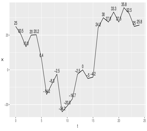
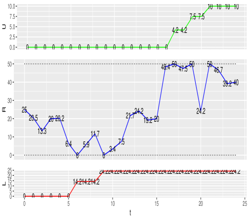
Figure 1: The Skorohod map in terms of random walks. Left panel: unrestricted Lévy walk sample trajectory with $R(0)=X(0)=25$ and the number $N=24$ of consecutive ”time” steps (e.g. displacements $Y(i)$). Right panel depicts a construction of the Skorohod triplet $R,L,U$, where $R$ stands for a reflecting Lévy random walk in $[0,50]$, started at $X(0)=25$. The compensating walks (e.g. lower $L$ and upper $U$ regulators) are inferred from the data of the unrestricted process, by means of the recursion (24).

The Skorohod map is detailed in Fig. 1. The reflecting Lévy walk is inferred from the standard unrestricted Lévy walk, as introduced in Eq. (20), in accordance with the concept of the Skorohod map. We note that integer labels $k$ effectively correspond to normalised (length $1$) ”time” steps. Indeed, it is enough to consider a test time interval $[0,T]$, which is composed of $N$ integer ”time” points, so that we deal with normalized increments $t_{i}-t_{i-1}=1$ for each value of $1\leq i\leq N$. We note that the scaling (19) is here immaterial, because $(t_{i}-t_{i-1})^{1/\alpha}=1$.

We choose $N=24$ and create a sample trajectory of the unrestricted Lévy walk starting from the value $R(0)=25$, c.f. (24). Since $X(1)=20.5$, we get $Y(1)=-4.5$. In the left panel of Fig.1 the sample path of our walk is represented by randomly assigned jumps, which produce coordinate labels with values along the vertical axis. So e.g. consecutive jumps $-4.5;-7.2;+6.7;+0.2;-13.8;$ etc., give rise to the unrestricted random walk steps $20.5;13.3;20;20.02;6.4$ etc., as depicted in the panel.

To realize the Skorohod map, we actually need to properly ”tailor” the obtained unrestricted sample trajectory, so that it will fit to the a priori chosen residence interval $[0,b]$ with $b=50$ of the prospective two-sided reflected Lévy walk. This is detailed in the right panel of Fig.1, in terms of two compensating random walks: (i) the upper barrier regulator $U(N)$ (green) and (ii) the lower barrier regulator $L(N)$ (red).

To implement the reflecting walk we employ the recursion formula (24), where the regulators are visually absent. However, we can reconstruct them (this is the essence of the Skorohod map) as follows.

In the $6$th displacement step, the unrestricted process induces a jump $-20.6$ from $6.4$ to $-14.2$. According to Eq. (24) the jump is interrupted (stopped) at $0$, while the remaining part $-14.2$ must be compensated by the increase (jump from $L(5)=0$ to $L(6)=+14.2$ of the regulator $L$, which is depicted in red in the right panel. We have reached the value $R(6)=0$, beginning from which two consecutive jumps of the unrestricted process, $+5.8$ and $+5.9$, do not induce any increment of $L$, and ultimately $R(8)=11.7$.

However the trajectory of the unrestricted process, at the $9$th ”time” step jumps down by $-21.7$. On the level of reflected process $R$, according to Eq. (24), such jump from the value $R(8)=11.7$ is interrupted (stopped) at the value $R(9)=0$, and the regulator $L$ is activated again. This means that the compensating jump of the size $21.7-11.7=10$ needs to be executed, thus setting the value of the lower regulator at $L(9)=24.2$. This value is preserved up to $L(24)$.

We proceed analogously with the upper regulator, whose value equals zero up to the $17$th ”time” step, when the ”overshoot” occurs and upper value $R(17)=50$ is reached while executing the jump $+5.8$ from $R(16)=48.4$. The overshooting surplus $5.8-1.6=4.2$ is depicted as the value $U(17)$. Further procedure follows analogously.

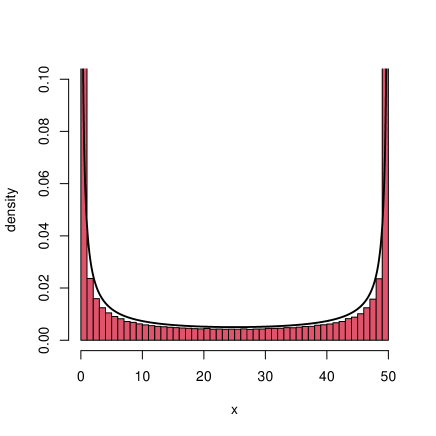
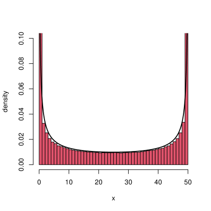
Figure 2: Skorohod random walk. Statistics (histograms) of $500000$ sample trajectory location ”hits” at $T=2500$, for $\alpha=0.3$ (left panel)and $0.7$ (right panel). All trajectories were started at $X(0)=25$. A continuous best fit curve, actually coincides with the singular $\alpha$-harmonic function of Eqs. (9), known to solve Eq. (11) in the (open) interval $(0,b=50)$, c.f. [34].

III.3 Skorohod random walk. Large time asymptotics and approximate stationary probability densities.

We are interested in statistical properties (strictly speaking, in inferred probability density functions), induced by the discretized (random walk) representation of solutions to stochastic differential equations with two-sided reflection constraints. To this end we divide the time interval $t\in[0,T]$ into $N$ equal segments, so that each time instant $t_{i}>0$ is a natural number, and $t_{i}-t_{i-1}=1$ for all $i$. This allows to neglect scaling issues of Eq. (19). We are interested in the (sufficiently) large time asymptotic, hence in statistical data (histograms of trajectory hits) for large values of $T$. Our test choice has been $T=2500$. We remember that for each spatial increment, see e.g. Eqs. (20), (21), there holds $Y_{i}\sim S_{\alpha}(1)$.

In Figs. 2-4 we depict the statistical data (histograms) at $T=2500$, inferred for $500000$ sample trajectories of the Skorohod random walk in the interval $[0,50]$, all started at $X(0)=25$, and generated for selected values $\alpha=0.3,0.7,1,1.3,1.7$ of the stability parameter. The continuous curve depicted in black, appears to be a definite best fit probability density function, actually coinciding with the singular $\alpha$-harmonic function of Eqs. (9), c.f. also (11).

A compatibility of histograms for the Skorohod random walk in the reflecting interval with the approximating continuous curve (9) is quite satisfactory, even for normalized time increments. The approximation finesse can be easily improved, if to generate trajectories with time increments significantly less than one (we need $\sim S_{\alpha}(\sigma)$, $\sigma<1$). This would increase the computer time cost, even while keeping fixed $T=2500$.

We have explicitly tested the finesse improvement, by passing to the time increment equal $1/8$. The comparative outcome is depicted in Fig. 3 for $\alpha=1.7$ and $T=2500$. An approximation accuracy improvement can be visually verified. Analogous comparative tests are depicted in Fig.4 for $\alpha=0.3,1,1.7$.

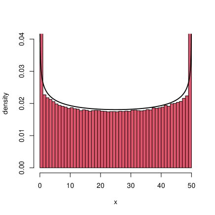
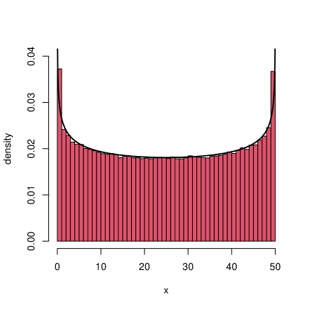
Figure 3: Statistics (histograms) of $500000$ trajectories generated for $\alpha=1.7$, using a normalised (equal $1$ in the left panel) time increment, and comparatively (to indicate a visually significant increase of the approximation finesse) for its $1/8$ version (right panel). A continuous curve coincides with this of Eq. (9), for $b=50$.

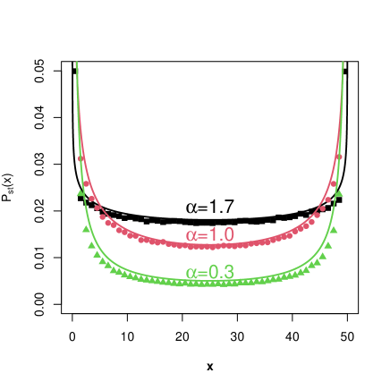
Figure 4: Skorohod random walk. A comparative statistics for $500000$ trajectories, generated for $\alpha=0.3,1,1.7$, with the unit time increment (left panel) and its $1/8$ version. Coordinates of each displayed dot (triangle, square, circle) are specified as follows: abscissa axis specifies histogram midpoints, while the ordinate axis refers to probability density (actually the frequency of trajectory ”hits”). The starting point $X(0)=25$ is common for all trajectories. The continuous curve (9) is displayed in black.

IV Beyond the Skorohod map. Alternative reflection scenarios at a barrier.

IV.1 Interception, or stopping at the barrier.

The discretisation of the form (24) of $R(t)$, without explicit reference to the Skorohod problem, can be found as Eq. (10) in Ref. [43], in connection with the reflection scenario from a single barrier located at $w>0$, with the forbidden region $x<w$ (actually $w$ can be identified with $0$). Then the recursion, originally carried out with reference to the increments $\xi$ of the fractional Brownian motion, [43], (with no abuse of notation we can interpret $\xi$ as increments of the standard Brownian motion or any $\alpha$-stable Lévy process)

$$x_{n+1}=\max(x_{n}+\xi_{n},w)$$ (25)

places the particle right at the barrier, if the step would take it into the forbidden region $x<w$. Clearly, we encounter an interception of the ”overshooting” jump by the barrier. This (barrier) stopping location is the starting point for the consecutive jump. If the jump would potentially take the trajectory to the forbidden region, it is not realised and the barrier location remains the stopping point, until a ”proper” jump gets sampled.

The definition (24) has been interpreted as a discretised version of the reflecting behavior in the fractional Brownian motion (FBM). It is often employed in the mathematical literature, in the context of queueing theory [46, 47], and likewise for Lévy processes, [24, 25, 26].

Reflections (25) from the bottom barrier $w\in R$, can be readily transcribed to the Lévy setting by means of obvious substitutions (compare e.g. Eq. (24)), resulting in:

$$R_{n}=\max(w,R_{n-1}+Y_{n})$$ (26)

Formulas for the upper barrier readily follow. Eq. (24) actually combines the bottom and upper barrier cases in a single recursion formula, for the Lévy walk with reflections at endpoints of the interval, $[0,b]$, where $w=0$ stands for the lower barrier. This is consistent with the two-sided (Skorohod) reflection scenario and the asymptotic behavior of probability distribution inferred from the statistics of a large number of random paths, as reported in Figs. 2, 3 and 4, with an approximating pdf of Eq. (9).

Remark: Under the name of the ”motion stopping” scenario, a very similar proposal has been employed in Ref. [30]. In reference to the interval $[0,b]$, a trajectory that crosses $0$ is paused at $+\epsilon>0$, which is supposed to be small. The point $+\epsilon$ is used as a starting point for the next jump. Clearly, if the consecutive jump would possibly ”overshoot” $+\epsilon$ in the negative direction, the motion would remain stopped until the move in the positive direction is enabled again. A closer examination proves that this $\epsilon$-stopping scenario is equivalent to the Skorohod random walk in the $2\epsilon$ - reduced interval $[\epsilon,b-\epsilon]$. In Ref. [30], the Authors have chosen $\epsilon=0.001$, [32]. Monte carlo simulations have confirmed that the curve (9) is a reliable continuous approximation of the statistical (histograms) data for asymptotic probability distributions in the pertinent random walk.

IV.2 Wrapping and mirror reflection.

Another reflection scenario proposal, restricting the random walk to $x\geq w$ can be defined by means of a recursion:

$$x_{n+1}=w+|x_{n}+\xi_{n}-w|,$$ (27)

which for $w=0$ is recognizable as the standard (Brownian by origin) reflection from an ”elastic” wall. For $w>0$, the reflection formula (27) describes the wrapping scenario , c.f. [31], where a sample trajectory that would potentially end at $x<w$, actually is wrapped around $w$ and the ”jump length surplus” $|x-w|$ is added to $w$ to get the final outcome (e.g. reflection through wrapping). We note that for $w=0$, and $x_{n}>0$, we have $x_{n+1}=|x_{n}+\xi_{n}|$, which is a mirror reflection at $0$.

Remark: We recognize in Eq. (26) the wrapping scenario of reflection from the lower barrier, originally adopted to the interval $[-L,L]$, in which the $\alpha$ - stable process was supposed to be confined. In this case, the numerically assisted statistical analysis, has revealed that the asymptotic probability density function needs to be a constant, [32].

For the Lévy walk subject to the mirror reflection scenario at the endpoints of $[0,b]$, we shall explicitly demonstrate signatures of convergence to a constant distribution in Fig. 4. That remains in conformity with the spectral analysis of the regional fractional Laplacian, outlined in Ref. [1], see also [29].

Figure 5: Mirror reflection in $[0,50]$. Statistics of $500000$ trajectories for $\alpha=0.3$ and the normalized time increment. All trajectories have a common starting point $X(0)=25$.

For the reader convenience, we outline our procedure in the mirror case, when the lower barrier is set at $0$, the interval of interest is $[0,b]$, with $b=50$, and $X(0)=25$ is chosen as the starting point of the random walk.

For the $\alpha$-stable Lévy process, we define the mirror reflection from the lower barrier at $0$ as follows:

$$R_{n}=|R_{n-1}+Y_{n}|.$$ (28)

Here $n=1,2,\ldots$, and $R(0)=X(0)=b/2$, compare e.g. [43, 31]. The upper barrier we set at $b$. To arrive at a mirror reflection, we modify appropriately the reflection recipe (27):

$$R_{n}=w-|R_{n-1}+Y_{n}-w|$$ (29)

To arrive at a consistent two-sided reflection in $[0,b]$, we need to keep resultant $R_{n}\in[0,50]$, while remembering that the increments $Y_{n}\sim S_{\alpha}(1)$ are a priori unrestricted in size.

We proceed as follows. Each random outcome $R_{n}$ we evaluate in terms of modulo operation with respect to division by $2b$. This guarantees, that jumps of size exceeding $2b$ will be mapped back (actually the remainder of the division by $2b$) to the interval $[0,2b)$. In passing we note, that the jump from $0$ by an integer multiple of $2b$, if interpreted modulo $2b$, would always land at $0$.

Accordingly, if $Y_{n}\geqslant 0$,then $R_{n}=R_{n-1}+Y_{n}$ only if $R_{n-1}+Y_{n}<b$. On the other hand, if $R_{n-1}+Y_{n}\geqslant b$, then the admissible outcome is $R_{n}=|2b-R_{n-1}-Y_{n}|$.

For $Y_{n}<0$, we admit $R_{n}=R_{n-1}+Y_{n}$ only if $R_{n-1}+Y_{n}>0$. If this is not the case, we accept the outcomes according to: (i) if $|R_{n-1}+Y_{n}|<b$, then $R_{n}=|R_{n-1}+Y_{n}|$, (ii) if $|R_{n-1}+Y_{n}|\geqslant b$, then $R_{n}=2b-|R_{n-1}+Y_{n}|$.

So defined random walk ”evolution” leads to the uniform distribution on $[0,b]$, as anticipated. In Fig. 5 we depict results of the simulation of $500000$ trajectories of the pertinent reflected random walk, for $\alpha=0.3$ at $T=2500$. For other exemplary values of $\alpha$ the outcome (uniform distribution) is the same.

IV.3 Apprehensive stopping. Skipping the forbidden jump.

Eq. (9) of Ref. [43] provides another recursion formula, used to simulate the reflection from the bottom barrier ($x\geq w$) in a number of recent publications on the reflected fractional Brownian motion, [41]-[45]. We stress that there is no unique, universally accepted reflection form the barrier scenario. In contrast to (25) the original recursion formula of the random walk:

$$x_{n+1}=x_{n}+\xi_{n}\,;\,\,\,\,x_{n}+\xi_{n}\geq w$$

$${x_{n+1}=x_{n}\,;\,\,\,\,x_{n}+\xi_{n}<w}.$$ (30)

defines an “inelastic” wall at which the there is no move (jump) at all from the achieved ”location” $x_{n}$, if the step would ultimately take it into the forbidden region $x<w$. The barrier is never ”overshot”, may merely be reached.

The above scenario can be readily adopted to the Lévy walk case. With $X(n)=X_{n}$ defined by (20), we generate the reflected process $R_{n}$ following (30):

$$R_{n}=R_{n-1}+Y_{n}\,;\,0\leqslant R_{n-1}+Y_{n}\leqslant b.$$ (31)

If the above inequality is not satisfied, we keep $R_{n}=R_{n-1}$. e.g. skip the barrier overshooting jumps.

The statics of ”hits” of $500000$ sample paths at ”time” $T=2500$ (with a normalised time increment) undoubtedly reveals that the asymptotic distribution is uniform in the interval $[0,50]$. The result is $\alpha$-independent, and is depicted in Fig. 6 for $\alpha=0.3,1.0,1.7$.

Figure 6: Apprehensive stopping in $[0,50]$. Statistics of $500000$ trajectories for $\alpha=0.3,1.0,1.7$, with $R(0)=25$. Random walk signatures of the uniform distribution.

To confirm the distribution uniformity, we can also proceed by evaluating the second moment $<R^{2}(t)>$ for the trajectory statistics, as a function of time. The (expected to be) limiting value of $<R^{2}>$ in the case of the uniform distribution on $[0,b]$ is $b^{2}/3$, e.g. about $833.(3)$ for $b=50$.

For each trajectory started from $R(0)=25$ , after few time steps we identify oscillations about $833$, which die out with the growth of the number of trajectories, for which statistical data are gathered. This is independent of the particular choice of $\alpha$.

In passing,we mention that in Ref. [43] (Fig. 1 therein) it has been shown that for the fractional Brownian motion (FBM) the mean value of the squared distance, in the large time asymptotic exceeds that for the uniform distribution. For the considered Lévy walk such behavior has not been found, which supports our conjecture about the uniformity of the probability distribution in the large time limit for Lévy walks respecting the ”apprehensive stopping” scenario.

V Nonlocal analog of the Neumann condition: Path-wise implementation.

V.1 Fractional heat equation with the nonlocal Neumann condition.

In Ref. [1] we have considered seriously a hypothesis (see e.g. [13, 14]) that the regional fractional Laplacian might serve as a generator of reflected Lévy processes in the interval. This assumption motivated our discussion of section V there-in, devoted to signatures of the reflecting boundaries in the spectral problem for the regional fractional Laplacian. By employing the Neumann basis system in the corresponding state space, we have derived lowest eigenvalues and eigenfunctions, with the clear outcome that the ground state function is constant and corresponds to the eigenvalue zero. This observation stays in an obvious conflict with the formula (9), which has been attributed to the Lévy process in the interval as well, see e.g. also [1, 4, 36].

We have learned in the previous section that some of the path-wise reflection recipes may in principle lead to uniform probability distributions in the interval, at variance with the singular $\alpha$-harmonic function shape of Eq. (9). On the other hand, we have identified (9) as the best fit approximation of the Skorohod random walk, which provides a well defined process with reflections form the interval endpoints.

In the present section, we shall outline rudiments of another ”reflecting” framework for Lévy processes in the interval, with the fractional heat (Fokker-Planck) dynamics leading asymptotically to the uniform distribution. Its major ingredient is the so-called nonlocal Neumann condition [16, 17, 3, 18]. We note that there are other Neumann condition proposals in existence, [14, 15] and [13], but transparent probabilistic pictures, amenable to a computer-assisted (path-wise) verification, appear to be lacking.

The nonolocal Neumann condition of Ref. [16] allows to bypass these limitations. We provide a brief resume of main results of Ref. [16], which is free of (unnecessary here) technical details.

Let us come back to an integral definition of the fractional Laplacian (13), while reintroducing under the integral sign the numerator $f(x)-f(y)$ instead of $f(x)$ alone. We extend the domain for $f(x)$ to the whole real axis and remove the exterior Dirichlet restriction upon $f(x)$ from the discussion. This condition is removed as well from the identity (12), so that $(-\Delta)^{\alpha/2}f(x)=h(x)$. As a matter of principle, we may extend the reasoning to the time-dependent problem, with $f(x)\equiv f(x,t)$, $h(x)\equiv h(x,t)$, while assuming an initial condition $f(x,0)=f_{0}(x)$. Accordingly, by setting $h(x,t)=-\partial_{t}f(x,t)$, we arrive at the fractional Fokker-Planck type equation in $R$

$$\partial_{t}f(x,t)=-(-\Delta)^{\alpha/2}f(x,t).$$ (32)

At the moment this equation is unrestricted by any domain requirements, and the fractional Laplacian has a standard (Cauchy principal value) integral realization (7), (8), c.f. also (13).

A nonlocal analogue of the classical Neumann condition $\partial f(x)=0$, normally imposed at the boundary $\partial D$ of the set $D$, for Lévy processes consists in the nonlocal prescription, [16]:

$${\cal{N}}_{\alpha}f(x)={\cal{A}}_{\alpha}\,\int_{D}{\frac{f(x)-f(y)}{|x-y|^{\alpha+1}}}\,dy=0,$$ (33)

valid for all $x\in R\setminus\overline{D}$. We note that if the integral is restricted to $D=(0,b)$, the Neumann condition takes the value zero for all $x\in(b,\infty)$. An insight into the behavior sharply at the the boundary point $b$, needs a careful execution of limiting procedures from the interior of $[b,\infty)$ toward $b$, [16]. The validity of (33) extends to the time-dependent regime $f(x)\to f(x,t)$ as well.

Eqs. (32) and (33), together with the initial data $f_{0}(x)$, constitute a heat equation with homogeneous Neumann conditions, according to Ref. [16]. The system, although defined on $R$ has a number of interesting properties related to the opens set $D$, like e.g. ”mass” (probability or initial normalization) conservation inside $D$, and convergence to a constant (uniform distribution) as $t\to\infty$. Moreover, the spectral problem for the fractional Laplacian with the boundary condition (33) has a solution such that $(-\Delta)^{\alpha/2}u_{i}(x)=\lambda_{i}u_{i}(x)$ for any $x\in D$ and ${\cal{N}}_{\alpha}u_{i}(x)=0$ for any $x\in R\setminus\overline{D}$. The eigenvalues are nonnegative, and the bottom one equals zero. The eigenfunctions, if restricted to $D$, form a complete orthogonal system in $L^{2}(D)$.

There is a transparent probabilistic interpretation behind the formal setting (32), (33). Namely, if $u(x,t)$ is a probability density function of a random process inside $D$, any exit beyond $D$ is immediately followed by a return to $D$. The way, the process comes back to $D$ according to the randomized wrapping rule: an immediate return from the ”overshot” destination $x\in R\setminus\overline{D}$ is random and gets realised with the return probability of jumping from $x$ to any $y\in D$, which is proportional to $|x-y|^{-1-\alpha}$. (We recall that for the unrestricted Lévy process,a jump from $x\in R$ to any other point $y\in R$ is realised with the probability of jumping being proportional to the invoked $|x-y|^{-1-\alpha}$).

We have coined the term randomized wrapping to set a correspondence with the wrapping scenario of Section IV.B, in which the return to $D$ is realised in the single run: start from $D$, overshoot the barrier, immediately return back to $D$. This tells us what might mean the ”immediate return” in the nonlocal Neumann problem. A mirror reflection is another example of such (albeit non-random) ”immediate return”.

V.2 Instantaneous randomized wrapping.

We have not found in the literature any explicit path-wise analysis of the above reflection scenario, hence we shall spend a while on its somewhat detailed discussion.

For a symmetric $\alpha$-stable Lévy process $\{X(t),t\geqslant 0\}$, its random walk version $X_{n}$ is generated according to (20). The reflection scenario, we attempt to visualise by following the heuristics of Ref. [16], appears to be a randomised version of the previously discussed wrapping scenario. Namely, we assume that the trajectory never actually leaves the interval $[0,b]$. All exits (potential overshooting the barier) are virtual. The starting point is $R(0)=b/2$.

We proceed as follows:
a) If $0\leqslant R_{n-1}+Y_{n}\leqslant b$ then we accept the jump $R_{n}=R_{n-1}+Y_{n}$.
b) If the sampled jump would be long enough to overshoot $b$, reaching a destination $y>b$, then the immediate return (jump) is executed from the coordinate $y$ to certain $x\in D=[0,b]$, with a conditional probability proportional to $|x-y|^{-1-\alpha}$.

We note that the virtual exit $y$ from $[0,b]$ is followed by an immediate return to a certain $x\in[0,b]$ in the single run (e.g. uninterrupted jump). The return is immediate in analogy with the execution of overshooting jumps in the wrapping scenario of subsection IV.B. Therefore, we call the current scenario the randomized wrapping about the barrier.

The probability density of jumps from a virtual point $y\in R\setminus\overline{D}$, to any $x\in D$. we denote $\rho_{y}(x)=C|x-y|^{-1-\alpha}$. We need to evaluate the $L^{1}([0,b])$ normalizing coefficient $C$. This must be done separately for the upper and lower barriers.

Let $y>b$, then

$$C\int\limits_{0}^{b}|x-y|^{-1-\alpha}\,dx=\frac{C}{\alpha}\frac{y^{\alpha}-(y-b)^{\alpha}}{[y(y-b)]^{\alpha}}=1\Longrightarrow C=C_{b}=\frac{\alpha[y(y-b)]^{\alpha}}{y^{\alpha}-(y-b)^{\alpha}}.$$ (34)

An analogous evaluation for $y<0$ gives rise to $C=C_{0}$ equal

$$C=C_{0}=\frac{\alpha[y(y-b)]^{\alpha}}{(b-y)^{\alpha}-(-y)^{\alpha}}.$$ (35)

The respective probability densities $\rho_{y>b}(x)$ and $\rho_{y<0}(x)$ directly follow.

Given the probability density $\rho_{y}(x)$ of return to $D=[0,b]$ from any $y\in R\setminus\overline{D}$, we need to implement a fully fledged randomisation of return points $x\in D$, for each virtual $y$ separately, while accounting for the barrier (bottom or upper) location in $R$. To this end, we invoke the inverse cumulative distribution function (ICDF) method, which is a widely recognised procedure allowing to generate random samples, that are consistent with any prescribed probability distribution, [58] Chap. II.

Given $y>b$, to deduce the random return coordinate $x\in D$ (”reflection” point for a jump turned back at $y>b$ ), let us denote $p$ a value of the random variable $U$ sampled from the uniform distribution on $[0,1]$. We require that each sampled $p\sim U(0,1)$ is uniquely assigned to the return point $x\in D$. This we secure in terms of the cumulative probability distribution evaluated up to the point $x$:

$$\int\limits_{0}^{x}\rho_{y>b}(z)\,dz=p.$$ (36)

To infer the return coordinate $x\in[0,b]$ of the completed jump (overshooting and random return) of the sample trajectory, we must employ the inverse function $F^{-1}_{X}(p)=x$, which uniquely identifies $x\in D$, given $p\in[0,1]$. This randomization procedure refers to each wrapping point $y>b$ separately.

We have

$$C\int\limits_{0}^{x}|z-y|^{-1-\alpha}\,dz=C\int\limits_{0}^{x}(y-z)^{-1-\alpha}\,dz=\frac{C}{\alpha}\left[(y-x)^{-\alpha}-y^{-\alpha}\right]=p.$$ (37)

After inserting $C=C_{b}$ of Eq. (35), we ultimately get

$$x=x_{b}=y-y\left[1-p+p\left(\frac{y}{y-b}\right)^{\alpha}\right]^{-1/\alpha}.$$ (38)

The random sampling of $p$ has been uniquely transferred to the randomness of $x$-outcomes. Indeed, for a uniformly distributed $p\in[0,1]$, the probability distribution of $X$ with values $x$ given by Eq. (38) has a probability density function $\rho_{y>b}(x)$.

Analogously, for $y<0$ the jump return destinations $x\in[0,b]$, derives as

$$x=x_{0}=y-y\left[1-p+p\left(\frac{-y}{b-y}\right)^{\alpha}\right]^{-1/\alpha}.$$ (39)

Random outcomes $x_{0}$ and $x_{b}$, can actually be obtained from a formula, encompassing both cases. Indeed, the random return jump location $x=x(y)$ is given by a compact formula

$$x=x(y)=y-y\left[1-p+p\left|\frac{y}{y-b}\right|^{\alpha}\right]^{-1/\alpha},$$ (40)

for each $y\notin[0,b]$ and each preassigned (sampling from a uniform distribution) value of $p$.

With these preparations, we are finally ready to accomplish the visualisation of the random wrapping reflection scenario, according to Ref. [16]. Steps a) and b) described above are now completed by one more step:
c) If $y=R_{n-1}+Y_{n}$ is beyond $[0,b]$, then the final destination of the jump, originating from $R_{n-1}$ (jump with wrapping return), is given by $R_{n}=x$, where $x$ stands for the random coordinates in $D$, which is uniquely related to a pre-sampled value of $p\sim U(0,1)$, c.f. .

In Fig. 7 we have depicted a statistics of $500000$ trajectories of times span $T=2500$, with the normalised time step, choosing $b=50$ and following the reflection scenario a) to c), for $\alpha=0.3,1,1.7$.

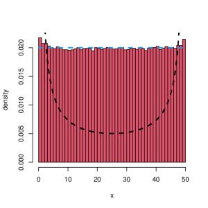
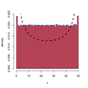
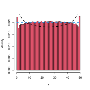
Figure 7: Randomised wrapping. Statistics of $500000$ trajectories for $\alpha=0.3,1,1.7$. The starting point is $v=25$. The black dashed curve comes from the formula (10) and is introduced for reference. The green line indicates an approximating uniform distribution $U(0,50)$. This result is consistent with the asymptotic behavior of the solution of the fractional heat equation with the nonlocal Neumann condition, Eqs. (32), (33).

For $\alpha=0.3$ (left panel in Fig.7) the distribution is fapp (for all practical purposes) constant on $[0,50]$, except for a close vicinity of the interval endpoints, where frequency histograms slightly grow with a diminishing distance. This behavior can be interpreted as follows. For small $\alpha$ long jumps are relatively frequent, so that quite often their virtual destinations are beyond $[0,b]$. The randomised wrapping and return of the jump to $[0,b]$ is ruled by the probability density $\rho(x|y)$, which appears to favor final destination close to the endpoints, against these close to the central part of the interval.

On the other hand, for $\alpha=1.7$ (right panel in Fig. 7) frequency of long jumps is significantly reduced and statistically important virtual overshoots of the barriers are dominated by these originating from points close to barrier in the interior of $[0,b]$. The random returns do not seem to compensate the probability loss near the barriers, and contribute to the remaining part of $[0,b]$. The case of $\alpha=1$ appears to be transitional in this respect, and shows a mutual compensation of the outlined before ($\alpha=0.3$ vs $\alpha=1.7$) probability redistribution tendencies.

Anyway, the theory of Ref. [16] says that in the long time asymptotic, the uniform distribution should be ultimately reached for all $\alpha\in(0,2)$.

V.3 Alternative model. Delayed (separate run) randomised return.

Simply, out of curiosity, let us consider a modification of the previous scenario, which might have some realistic physical appeal. Let us admit the overshooting is a realistic event, and the path exits form $D$ to the exterior point $y$. To divert the trajectory back to $D$, we presume to need a separate (randomized) jumping event, with the jump length ruled by the probability density $\rho_{y}(x)$ of the previous subsection.

All formulas of the previous subsection retain their validity, except that $y$ is not a virtual point, but a real destination of the overshooting jump through any barrier of $[0,b]$. Consequently, the exit point $y$, in the next time step becomes a starting point for the independent jump (with length randomized according to $\rho_{y}(x)$), sending the trajctory back to $[0,b]$.

Statistical data for $500000$ trajectories, generated with a normalised time step, and $b=50$, have been collected accepting the delayed reflection scenario, for $\alpha=0.3,1,1.7$. These are depicted in Fig. 8.

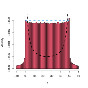
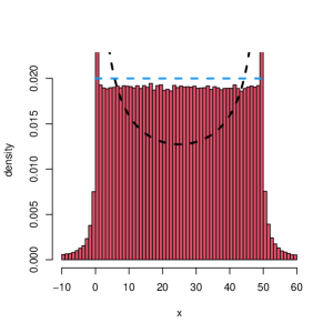
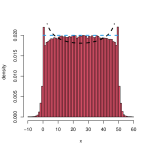
Figure 8: Delayed randomized return. Statics of $500000$ trajectories for $\alpha=0.3,1,1.7$. Trajectories are started at $x=25$. Black dashed curve depicts the reference curve (9) for $b=50$, while the green dashed line refers to the uniform distribution $U(0,50)$.

Qualitatively, the statistic (histograms) of hits at time $2500$, are close to these produced in the randomized wrapping reflection of the Subsection V.B. Beacuse we allow trajectiories to leave $D$, with return in the next time step, there are cleraly visible distribution ”tails”, beyond $[0,50]$. ”Heavy” (long) tails effects are clearly displayed, specifically for low value of $\alpha=0.3$, and their contribution gets minimized with the growth of $\alpha$.

If to rescale the time step form $1$ to $1/8$, we uncover a clear similarity (except for remnant distribution tails in close outside vicinity of the barriers) to the randomized wrappin results of Section V.B. The corresponding statistical data (histograms) for $500000$ trajectories are depicted in Fig. 9.

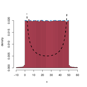
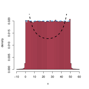
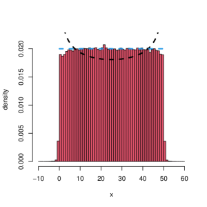
Figure 9: Delayed return. Statistics (histograms) of $500000$ trajectories for $\alpha=0.3,1,1.7$, with the time step rescaled to $1/8$. Trajectories start from $x=25$. The black curve refers to Eq. (9), while the green dashed line depicts the uniform distribution $U(0,50)$.

Accordingly, with the small time step, statistical data for the Lévy walk with the randomized wrapping at barrier, become fapp (for all practical purposes) indistinguishable from these obtained in the delayed return scenario. Minor long tail remnants beyond the barriers, for a large number of time steps and the ”small time increment” discretization, practically may be absorbed in the ”discretisation inaccuracy” estimates.

VI Conclusions.

Essentially new results in our path-wise analysis of Lévy random walks (interpreted as time-discretizations of regular $\alpha$-stable Lévy processes), are contained in Sections III and V. Arguments of Section IV give a supplementary view upon path-wise reflection scenarios employed in the current physics-oriented research (in reference to both the fractional Brownian motion, [41]-[45], and Lévy flights proper, [30]-[33]).

Instead of imposing the boundary restrictions upon fractional motion generators (c.f. Section II), we have started from the Lévy random walk approximation of $\alpha$-stable jump-type processes on $R$. In section III, an explicit random walk construction of the Skorohod reflection process in the interval has been performed. We have obtained convincing statistical data about confining properties of this walk. The asymptotic pdf (its histogram) is satisfactorily approximated by the singular $\alpha$-harmonic function (9) (deduced by other means in Ref. [33]). The approximation accuracy can be improved while increasing the time-span of the walk and improving the discretization finesse of time-increments. To our knowledge, for the first time an explicit functional form of the asymptotic pdf has been associated with the Skorohod random walk.

As indicated in Section IV asymptotic pdfs are quite sensitive to the choice of a concrete reflection-at-the-barrier scenario. The stopping procedure of Section IV.A implies the singular $\alpha$-stable pdf on the trajectory statistics level. The procedure of [30] stays in close affinity with that scenario and in fact is a realisation of the Skorohod reflecting walk in the interval reduced by $2\epsilon$. To be more concrete, instead of the reference interval $[0.50]$ employed by us in Section III, one bypasses the problem that (9) is a valid harmonic function in the interval $(0,50)$, being equal to zero in $R\setminus(0,50)$, by considering (effectively) the Skorohod random walk problem in the interval $[\epsilon,50-\epsilon]$, where $\epsilon=0.001$, [32].

Other popular reflection scenarios (Sections IV.B and IV.C) induce uniform asymptotic pdfs in the interval (this is consistent with spectral solutions for the regional Laplacian, [1]).

In Section V we have discussed the nonlocal Neumann condition proposal of Ref. [16, 17, 18], presenting an explicit construction of the related random walk, in conjunction with the asymptotic pdf data. By theory of [16], the pertinent pdf should be uniform in the interval. Our statistical analysis is compatible with the result.

As an alternative reflection scenario (this is not covered by the original paper [16], we have investigated the delayed randomized Lévy walk whose sample paths are allowed to exit the confining interval, but in the next time step (that is the delay) they return back to the pertinent interval, according to the random rule of Section V.A. The resultant asymptotic pdf shows signatures of uniformity in the interval, with fapp (for all practical purposes) negligible long-tail remnants in the close outside vicinity of the interval endpoints.

We point out that the explicit solution of the Skorohod random walk problem in the interval, allows to resolve a conundrum [1, 4] arising in connection with derivations of the formula (9) in Ref. [33]. Namely, the reasoning of [33] begins from assuming the validity of the exterior Dirichlet boundary data for the fractional Laplacian in the (open) interval. It is well known, that so restricted fractional Laplacian, admits well defined strictly positive (eigenvalues) spectral solution, with bounded eigenfunctions, [55, 56, 57] and [48]-[52]. We realize that (9) is an example of the unbounded function.

Uniform probability distributions in the interval, can be consistently related with regional fractional Laplacians, [1, 28, 29] and the nonolocal Neumann condition of Ref. [16]. In these cases, one may deduce spectral solutions with the bottom eigenvalue zero and a constant eigenfunction.

In our discussion, we have described the appearance of two basic types of asymptotic pdfs - uniform and singular (c.f. (9)) - which can be associated with the two-sided reflected Lévy process. We do not know of any other possibilities, but a discussion of censored Lévy processes in Ref. [13] seems to leave some (possibly narrow) room for other path-wise confinement scenarios, with potential consequences for the asymptotic pdf shapes. In our opinion the term ”reflection” still remains ambiguous therein. As well, we do not know of any explicit shape analysis of asymptotic pdfs for a family of reflected Lévy processes, analyzed in Ref. [14, 15], except for the statement that regional fractional Laplacians are appropriate motion generators. This however, might refer to uniform probability distributions in the interval, in conformity with arguments of Ref. [1], c.f. Section V therein.

References

- [1] P. Garbaczewski and V. Stephanovich, ”Fractional Laplacians in bounded domains: Killed, reflected, censored, and taboo Lévy flights”, Phys. Rev. E 99, 042126, (2019).
- [2] A. E. Kyprianou, Fluctuations of Lévy processes with applications, (Springer, Berlin, 2014).
- [3] M. Daoud and E. H. Laamri, ”Fractional Laplacians: A short survey”, Discrete & Continuous Dynamical Systems - S, 15(1), 95-116, (2022), doi:10.3934/dcdss.2021027
- [4] P. Garbaczewski and M. Żaba, ”Lévy flights in steep potential wells: Langevin modeling versus direct response to energy landscapes”, Acta Phys. Pol. B 51(10), 1965-2009, (2020).
- [5] P. Garbaczewski and V. Stephanovich, ”Lévy flights in confining potentials”, Phys. Rev. E 80, 031113, (2009).
- [6] E. V. Kirichenko, P. Garbaczewski, V. A. Stephanovich and M. Żaba, ”Lévy flights in an infinite potential well as a hypersingular Fredholm problem”, Phys. Rev. E 93, 052110, (2016).
- [7] P. Bratley, B. L. Fox and L. E. Schrage, A guide to simulation, (Springer, New York, 1987).
- [8] A. Janicki and A. Weron, Simulation and chaotic behaviour of -stable stochastic processes, (Marcel Dekker, New York, 1994).
- [9] A. Janicki and A. Weron, ”Can one see -stable variables and processes ?”, Statistical Science, 9,(1), 109-126, (1994).
- [10] A. Weron and R. Weron, ”Computer Simulation of Lévy -Stable Variables and Processes”,in: Chaos - The interplay between stochastic and deterministic behavior, Eds. P. Garbaczewski, M. Wolf and A. Weron, (LNP vol. 457, pp. 379-392, Springer-Verlag, Berlin, 1995).
- [11] S. Asmussen and P. W. Glynn, Stochastics simulation. Algorithms and analysis, (Springer, New York, 2007).
- [12] P. Garbaczewski and V. Stephanovich, ”Lévy flights and nonlocal quantum dynamics”, J. Math. Phys. 54, 072103, (2013).
- [13] K. Bogdan, K. Burdzy, Z.-Q. Chen, ”Censored stable processes”, Probab. Theory Relat. Fields 127, 89 (2003).
- [14] Q.-Y. Guan, Z.-M. Ma, ”Reflected symmetric -stable processes and regional fractional Laplacian”, Probab. Theory Relat. Fields 134, 649 (2006).
- [15] Q.-Y. Guan, Z.-M. Ma, ”Boundary problems for fractional Laplacians”, Stoch. Dyn. 05, 385 (2005).
- [16] S. Dipierro, X. Ros-Oton, and E. Valdinoci, ”Nonlocal problems with Neumann boundary conditions”, Revista Matematica Iberoamericana, bf 33(2), 377-416, (2017).
- [17] A. Audrito, J-C. Felipe-Navarro and X. Ros-Oton, ”The Neumann problem for the fractional Laplacian: Regularity up to the boundary”, arXiv:2006.10026, (2020).
- [18] N. Abatangelo, ”A remark on nonlocal Neumann conditions for the fractional Laplacian”, Arch. Math. 114, 699, (2020).
- [19] N. Abatangelo, ”Large s-harmonic functions and boundary blow-up solutions for the fractional laplacian”, Discrete & Continuous Dynamical Systems, 35(12), 5555-5607, (2015).
- [20] M. Ryznar, ”Nontangential Convergence for -harmonic Functions”, in Potential Analysis of Stable Processes and its Extensions, edited by P. Graczyk and A. Stos, Lecture Notes in Mathematics Vol. 1980, Chap. 3, pp. 57-72, (Springer, Berlin, 2009).
- [21] A. V. Skorohod, ”Stochastic equations for diffusion processes in a bounded region”, Theory Probab. Appl., 6, 264–274, (1961).
- [22] A. V. Skorohod, ”Stochastic equations for diffusion processes in a bounded region. II”, Theory Probab. Appl., 7, 3-23, (1962).
- [23] A. Pilipenko, An Introduction to Stochastic Differential Equations with Reflection, (Potsdam: Potsdam University Press, 2014).
- [24] S. Asmussen, L. N. Andersen, S. Asmussen, P. W. Glynn, and M. Pihlsgård et al., ”Lévy processes with two-sided reflection”, in: Lévy Matters V. Functionals of L’evy Processes, Eds. L. N. Andersen et al., (LNM vol. 2149, pp. 67-182, Springer, Cham, 2015).
- [25] S. Asmussen and J. Ivanovs, ”Discretization error for a two-sided reflected Lévy process”, Queueing Systems, 89, 199-212, (2018).
- [26] S. Asmussen and M. Pihlsgård, ”Loss rates for Lévy process with two reflecting barriers”, Math. Operations Res. 32(2), 308-321, (2007).
- [27] Ł. Kruk, J. Lehoczky, K. Ramanan and S. Shreve, ”An explicit formula for the Skorohod map on ”, Ann. Prob. 35(5), 1740-1768, (2007).
- [28] I. A. Ibrahimov, N. V. Smorodina and M. M. Faddeev, ”Reflecting Lévy processes and associated families of linear operators”, Theory Probab. Appl., 64(3), 335-354, (2019).
- [29] P. Ievlev, ”Symmetric Lévy processes with reflection”, Global and Stochastic Analysis, 8(1), 25-40, (2021).
- [30] B. Dybiec, E. Gudowska-Nowak and P. Hänggi, ”Lévy-Brownian motion on finite intervals: mean first passage analysis”, Phys. Rev. E 73, 046104, (2006).
- [31] B. Dybiec, E. Gudowska-Nowak, E. Barkai and A. A. Dubkov, ”Lévy flights versus Lévy walks in bounded domains”, Phys. Rev. E 95, 052102, (2017).
- [32] B. Dybiec, private communication.
- [33] S.I. Denisov, W. Horsthemke and P. Hänggi, ”Steady-state Lévy flights in a confined domain”, Phys. Rev. E 77, 061112, (2008).
- [34] B. Dyda, ”Fractional calculus for power functions and eigenvalues of the fractional Laplacian”, Fract. Calc. Appl. Anal. 15(4), 536 (2012).
- [35] A. A. Kharcheva, A. A. Dubkov, B. Dybiec, B. Spagnolo and D. Valenti, ”Spectral characteristics of steady-state Lévy flights in confinement potential profiles”, J. Stat. Mech. 2016 054039.
- [36] P. Garbaczewski and M. Żaba, ”Brownian motion in trapping enclosures: steep potential wells, bistable wells and false bistability of induced Feynman–Kac (well) potentials”, J. Phys.A: Math. Theor. 53, 315001, (2020).
- [37] P. Garbaczewski, ”Killing (absorption) versus survival in random motion”. Phys. Rev. E 96, 032104, (2017).
- [38] A. Mazzolo, ”Sweetest taboo processes”, J. Stat. Mech. (2018) 073204.
- [39] J. Elliott and W. Feller, ”Stochastic processes connected with harmonic functions”, Trans. Amer. Math. Soc., 82, 392-420, (1956).
- [40] J. Elliott, ”The boundary value problems and semi-groups associated with certain integrodifferentialoperators”, Trans. Amer. Math. Soc. 76(2), 300-331, (1954).
- [41] T. Vojta, S. Skinner and R. Metzler, ”Probability density of the fractional Langevin equation with reflecting walls”, Phys. Rev. E 100, 042142, (2019).
- [42] T. Guggenberger, G. Pagnini, T. Vojta and R. Metzler, ”Fractional Brownian motion in a finite interval: Correlations effect, depletion or accretion zones of particles near boundaries, New J. Phys. 21, 022002, (2019).
- [43] T. Vojta et al., ”Reflected fractional Brownian motion in one and higher dimensions”, Phys. Rev. E 102, 032108, (2020).
- [44] A. H. O.Wada and T. Vojta, ”Fractional Brownian motion with a reflecting wall”, Phys. Rev. E 97, 020102(R) (2018).
- [45] A. Wada, A. Warhover, and T. Vojta, ”Non-Gaussian behavior of reflected fractional Brownian motion”, J. Stat. Mech.: Theory Exp. (2019) 033209.
- [46] J. Harrison, Brownian Motion and Stochastic Flow Systems, (Wiley, New York, 1985).
- [47] W. Whitt, Stochastic Process Limits, (Springer, New York, 2002).
- [48] M. Kwaśnicki, ”Eigenvalues of the fractional Laplace operator in the interval”, J. Funct. Anal. 262, 2379-2402, (2012).
- [49] T. Kulczycki, M. Kwaśnicki, J. Małecki, and A. Stós, ”Spectral properties of the Cauchy process on half-line and interval”, Proc. London. Math. Soc. 101, 589-622, (2010).
- [50] M. Kwaśnicki, ”Ten equivalent definitions of the fractional Laplace operator”, Fractional Calculus & Applied Analysis, 20(1), 7, (2017).
- [51] M. Kwaśnicki, ”Fractional Laplace operator and its properties”, in: ”Handbook of fractional calculus with applications”, vol. 1, (Eds. A. Kochubei and Y. Luchko, de Gruyter, Berlin, 2019).
- [52] T. Kulczycki, ”Eigenvalues and Eigenfunctions for Stable Processes”, chap. 4, pp. 73-86, in: K. Graczyk and A. Stos (Eds.), ”Potential Analysis of Stable Processes and its Extensions”, LNM vol. 1980, (Springer-Verlag, Berlin, 2009).
- [53] S. Duo, H. Wang and Y. Zhang, ”A comparative study of nonlocal diffusion operators related to the fractional Laplacian”, Discrete & Continuous Dynamical Systems - B 22(11), 1, (2018).
- [54] S. Duo and Y. Zhang, ”Computing the ground and first excited states of the fractional Schröodinger equation in an ininite potential well”, Commun. Comput. Phys., 18, 321-350, (2015).
- [55] M. Żaba and P. Garbaczewski, ”Solving fractional Schrödinger-type spectral problems: Cauchy oscillator and Cauchy well”, J. Math. Phys. 55, 092103, (2014).
- [56] M. Żaba and P. Garbaczewski, ”Nonlocally induced (fractional) bound states: Shape analysis in the infinite Cauchy well”, J. Math. Phys. 56, 123502, (2015).
- [57] E. V. Kirichenko, P. Garbaczewski, V. Stephanovich and M. Żaba, ”Ultrarelativistic (Cauchy) spectral problem in the infinite well”, Acta Phys. Pol. B 47(5), 1273-1291, (2016).
- [58] L. Devroye, ”Non-uniform Random Variate Generation”, (Springer-Verlag, Berlin, 1986).