Additional numerical and graphical evidence to support some Conjectures on discrete Schrödinger operators with a more general long range condition

Abstract.

This document contains additional numerical and graphical evidence to support some of the conjectures mentioned in [GM3]. We give more evidence for $\kappa=3,4$ in dimension 2. As mentioned in that article we still don’t quite understand the sets $\bm{\mu}_{\kappa}(\Delta)$ and $\bm{\Theta}_{\kappa}(\Delta)$ on $(0,1/2)$ for $\kappa=3$ in dimension 2. Here we give a bunch more threshold energies for $\kappa=3$ in dimension 2.

1. Introduction

The notation in this document is 100% consistent with that of [GM3]. We start by listing the 2 Conjectures of [GM3] for which the material presented in this document is relevant. The first has to do with the rate of convergence of the thresholds $\mathcal{E}_{n}\in J_{2}=J_{2}(\kappa):=\left(2\cos(\pi/\kappa),1+\cos(\pi/\kappa)\right)$.

Conjecture 1.1.

Let $\{\mathcal{E}_{n}\}$ be the sequence in [GM3, Theorem 1.7]. Then $\mathcal{E}_{n}-\inf J_{2}=c(\kappa)/n^{2}+o(1/n^{2})$, $\forall\kappa\geq 3$, where $c(\kappa)$ means a constant depending on $\kappa$.

For this conjecture, see section 2. The second conjecture has to do with the existence of a conjugate operator giving a strict Mourre estimate on bands $(\mathcal{E}_{n},\mathcal{E}_{n-1})\subset J_{2}$.

Conjecture 1.2.

Fix $\kappa\geq 2$. Let $\{\mathcal{E}_{n}\}$ be the sequence in [GM3, Theorem 1.7]. For each interval $(\mathcal{E}_{n},\mathcal{E}_{n-1})$, $n\geq 1$, $\exists$ a conjugate operator $\mathbb{A}(n)=\sum_{q=1}^{N(n)}\rho_{j_{q}\kappa}(n)A_{j_{q}\kappa}$, $A_{j_{q}\kappa}=\sum_{1\leq i\leq 2}A_{i}(j_{q},\kappa)$, such that the Mourre estimate for $\Delta$ holds wrt.  $\mathbb{A}(n)$, $\forall E\in(\mathcal{E}_{n},\mathcal{E}_{n-1})$. $\mathbb{A}(n)$ is typically not unique. It can be chosen so that $N(n)=2n$. In particular, $\{\mathcal{E}_{n}\}=J_{2}\cap\bm{\Theta}_{\kappa}(\Delta)$, $\forall\kappa\geq 2$.

For this conjecture, see sections 5, 6, 7 and 8. Section 4 lists some thresholds $\in\bm{\Theta}_{m=1,\kappa=4}(\Delta)$ in dimension 2, and section 9 gives a graphical illustration of some thresholds $\in\bm{\Theta}_{m,\kappa=3}(\Delta)\cap(0,1/2)$ in dimension 2, $m\geq 1$.

2. More evidence for the conjecture on the rate of convergence of $\mathcal{E}_{n}$

Figure 1 illustrates solutions $\mathcal{E}_{2n}(\kappa)$ of [GM3, Proposition 7.2] for $\kappa=5,6,8$. In these graphs the slope of the orange trend line is close to $-2$, and this is our rationale behind [GM3, Conjecture 1.9].

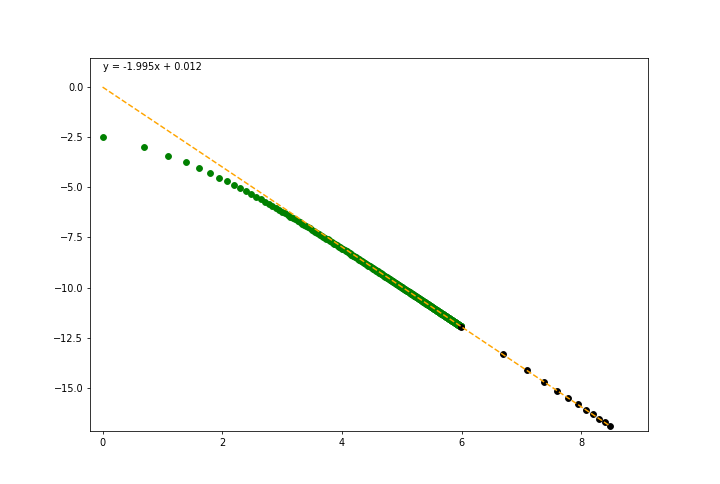
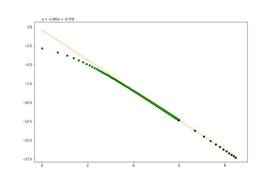
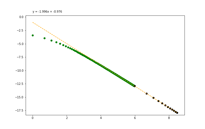
Figure 1. Graphs with $\log(n)$ on $x$-axis and $\log(\mathcal{E}_{2n}(\kappa)-2\cos(\pi/\kappa))$ on $y$-axis. Left : $\kappa=5$ ; Middle : $\kappa=6$, Right : $\kappa=8$. Green dots are $1\leq n\leq 400$ ; black dots are $n=400,800,1200,...,4800$. Orange line is trend line based on linear regression of black dots.

3. Energy solutions in $J_{2}(\kappa):=(2\cos(\pi/\kappa),1+\cos(\pi/\kappa))$

Table 1 below lists the first few energy solutions for $\kappa\in\{2,3,4\}$ in [GM3, Theorem 1.7]. In particular we have some exact expressions for $\kappa=4$.

$\kappa$	$\mathcal{E}_{5}$	$\mathcal{E}_{4}$	$\mathcal{E}_{3}$	$\mathcal{E}_{2}$	$\mathcal{E}_{1}$	$\mathcal{E}_{0}$
2	2/7	1/3	2/5	1/2	2/3	1
3	$\simeq 1.112$	$\simeq 1.137$	$\simeq 1.173$	$\frac{9+\sqrt{33}}{12}\simeq 1.228$	$\frac{5+3\sqrt{2}}{7}\simeq 1.320$	3/2
4	(7.4) $\simeq 1.476$	$\simeq 1.491$	(7.3) $\simeq 1.512$	(7.2) $\simeq 1.545$	8/5	$1+1/\sqrt{2}\simeq 1.707$

Table 1. First values of $\{\mathcal{E}_{n}\}$ in [GM3, Theorem 1.7]. $\Delta$ in dimension $2$. $\kappa=2,3,4$.

4. Thresholds in dimension 2, for $\kappa=4$, $m=1$ (the brute force approach)

In [GM3, subsection 4.2], we listed Ansatzes (1) – (6) to find threshold solutions $\in\bm{\Theta}_{1,\kappa}(\Delta)$, and in [GM3, Lemma 4.2] we listed those solutions for $\kappa=3$. Table 2 below lists the corresponding solutions for $\kappa=4$. We recall that these solutions belong to $\bm{\Theta}_{1,\kappa=4}(\Delta)$, but it is an open question for us if they constitute all of $\bm{\Theta}_{1,\kappa=4}(\Delta)$.

$\kappa$	$4$
(1)	$E=1/2+1/(2\sqrt{2})\simeq 0.853$, $Y_{1}=\sqrt{2}/2$
	$E=\frac{2+\sqrt{2}+\sqrt{2+4\sqrt{2}}}{4}\simeq 1.545$, $Y_{1}=\sqrt{2}/2$
	$E=\frac{2+\sqrt{2}-\sqrt{2+4\sqrt{2}}}{4}\simeq 0.161$, $Y_{1}=\sqrt{2}/2$
	$E=1/2-1/(2\sqrt{2})\simeq 0.146$, $Y_{1}=-\sqrt{2}/2$
	$E=8/5=1.6$, $Y_{1}=E/2=0.8$
(2)
(3)	$E=\sqrt{2/5}\simeq 0.632$, $Y_{1}=3/\sqrt{10}\simeq 0.948$
	$E=\sqrt{2}/3\simeq 0.471$, $Y_{1}=\sqrt{2}/2$
(4)	$E=2/\sqrt{5}\simeq 0.894$, $Y_{1}=0$, $Y_{0}=E/2\simeq 0.447$
	$E=1/\sqrt{5}\simeq 0.447$, $Y_{1}=0$, $Y_{0}=2E\simeq 0.894$
	$E=(\sqrt{3}-1)/(2\sqrt{2})\simeq 0.258$, $Y_{1}=0$, $Y_{0}=-\sqrt{2}/2$
	$E=1/(2\sqrt{2})\simeq 0.353$, $Y_{1}=0$, $Y_{0}=1/\sqrt{2}$
	$E=(\sqrt{2}+\sqrt{6})/4\simeq 0.965$, $Y_{1}=0$, $Y_{0}=1/\sqrt{2}$
	$E=3\sqrt{2}/5\simeq 0.848$, $Y_{1}=1/\sqrt{2}$, $Y_{0}=7/(5\sqrt{2})\simeq 0.989$
	$E=\sqrt{2}/5\simeq 0.282$, $Y_{1}=-1/\sqrt{2}$, $Y_{0}=E/2\simeq 0.141$
(5)
(6)

Table 2. Solutions to $(i)$, $1\leq i\leq 6$, in [GM3, subsection 4.2] for $\kappa=4$.

5. Polynomial Interpolation for the case $\kappa=2$ in dimension 2, $5\leq n\leq 9$

In [GM3, section 13] we gave numerical evidence of bands of a.c. spectrum for bands $n=1,2,3,4$, for $\kappa=2$ in dimension 2. We briefly mention that :

$\bullet$ For the $5th$ band, we checked that $\Sigma=[2,4,6,8,10,12,14,16,\alpha,\beta]$ is also valid for $(\alpha,\beta)=(18,20),(20,24),(22,24),(24,28),(24,32),(28,32)$ whereas it is not valid for $(\alpha,\beta)=(18,24)$, $(18,26),(18,28)$.

$\bullet$ For the $6th$ band we checked that $\Sigma=[2,4,6,8,10,12,14,16,18,20,\alpha,\beta]$ is valid for $(\alpha,\beta)=(22,28),(22,30)$ but not valid for $(\alpha,\beta)=(22,24),(22,26)$.

$\bullet$ For the $7th$ band we checked that $\Sigma=[2,4,6,8,10,12,14,16,18,20,22,24,\alpha,\beta]$ is valid for $(\alpha,\beta)=(26,28)$ but not valid for $(\alpha,\beta)=(28,36)$.

$\bullet$ For the $8th$ band we checked that $\Sigma=[2,4,6,8,10,12,14,16,18,20,22,24,26,28,\alpha,\beta]$ is valid for $(\alpha,\beta)=(30,38),(30,40)$ but not valid for $(\alpha,\beta)=(30,32),(30,36)$.

$\bullet$ For the $9th$ band we checked $\Sigma=[2,4,6,8,10,12,14,16,18,20,22,24,26,28,30,32,34,36]$ is valid.

6. Polynomial Interpolation for the case $\kappa=3$ in dimension 2, $n=5$

In [GM3, section 14] we gave numerical evidence of bands of a.c. spectrum for bands $n=1,2,3,4$, for $\kappa=3$ in dimension 2. We briefly give the numerical details for $n=5$, i.e. the $5^{th}$ band. $X_{3}=\mathcal{E}_{5}/2$ and

$$\begin{cases}T_{3}(\mathcal{E}_{5}-1)=T_{3}(\mathcal{E}_{5}-X_{1})&\\ T_{3}(X_{1})=T_{3}(\mathcal{E}_{5}-X_{2})&\\ T_{3}(X_{2})=T_{3}(\mathcal{E}_{5}/2)&\\ \end{cases}\Rightarrow\begin{cases}4\big{[}(\mathcal{E}_{5}-1)^{2}+(\mathcal{E}_{5}-1)(\mathcal{E}_{5}-X_{1})+(\mathcal{E}_{5}-X_{1})^{2}\big{]}=3&\\ 4\big{[}X_{1}^{2}+X_{1}(\mathcal{E}_{5}-X_{2})+(\mathcal{E}_{5}-X_{2})^{2}\big{]}=3&\\ 4\big{[}X_{2}^{2}+X_{2}(\mathcal{E}_{5}/2)+(\mathcal{E}_{5}/2)^{2}\big{]}=3.&\end{cases}$$

Using Python’s fsolve we get $[\mathcal{E}_{5},X_{1},X_{2}]\simeq[1.112,\ 0.307,\ 0.441]$. For an analytical solution or perhaps more precise, expand the equations and get rid of the $X_{1}^{2}$ and $X_{2}^{2}$ terms. One ends up with $4\left(9\mathcal{E}_{5}^{2}/4-4\mathcal{E}_{5}X_{1}+X_{1}X_{2}-3\mathcal{E}_{5}+1+5\mathcal{E}_{5}X_{2}/2+X_{1}\right)=3.$ Then use the fact that

$$X_{1}=-\frac{1}{2}+\frac{3\mathcal{E}_{5}}{2}-\frac{\sqrt{3}}{2}\sqrt{\mathcal{E}_{5}(2-\mathcal{E}_{5})},\quad X_{2}=-\frac{\mathcal{E}_{5}}{4}+\frac{\sqrt{3}}{4}\sqrt{4-\mathcal{E}_{5}^{2}}.$$

(signs are chosen based on numerical solution). We get an equation in $\mathcal{E}_{5}$ only, which is

$$0 =-(35\mathcal{E}_{5}^{2})/8+\left(3\mathcal{E}_{5}-\sqrt{3}\sqrt{(2-\mathcal{E}_{5})\mathcal{E}_{5}}-1\right)\left((1/8)\sqrt{3}\sqrt{4-\mathcal{E}_{5}^{2}}-\mathcal{E}_{5}/8\right)$$

$$\quad+(5/8)\sqrt{3}\mathcal{E}_{5}\sqrt{4-\mathcal{E}_{5}^{2}}+2\sqrt{3}\mathcal{E}_{5}\sqrt{(2-\mathcal{E}_{5})\mathcal{E}_{5}}+\mathcal{E}_{5}/2-1/2\sqrt{3}\sqrt{(2-\mathcal{E}_{5})\mathcal{E}_{5}}-1/4.$$

$\mathcal{E}_{5}$ is a root of

$$mp(E)=372775E^{8}-750010E^{7}+536359E^{6}-270784E^{5}+128593E^{4}-36442E^{3}+4333E^{2}-220E+4.$$

and we suspect it’s its minimal polynomial. $\mathcal{E}_{5}\simeq 1.11207$. We are not aware of a closed formula for $\mathcal{E}_{5}$. It follows that $X_{1}\simeq 0.30753$, $X_{2}\simeq 0.44178$, $X_{3}\simeq 0.55603$, $X_{4}\simeq 0.67028$, $X_{5}\simeq 0.80453$.

Next we suppose $\Sigma=[3,6,9,12,15,18,21,24,27,30]$. We fill the matrix $M$ with floats. Python says the solution to $M\rho=0$ is $[\rho_{3},\rho_{6},\rho_{9},\rho_{12},\rho_{15},\rho_{18},\rho_{21},\rho_{24},\rho_{27},\rho_{30}]^{T}$ equals

$$\simeq[1,1.599931,1.645307,1.27734,0.77838,0.37292,0.13741,0.03703,0.00657,0.00058]^{T}.$$

Graphically it seems $x\mapsto G_{\kappa}^{E}(x)>0$ for $E\in(\mathcal{E}_{5},\mathcal{E}_{4})$, $x\in[E-1,1]$. So $\Sigma$ is valid.

7. Polynomial Interpolation for the case $\kappa=4$ in dimension 2, $1\leq n\leq 6$

This section is the analogue of [GM3, section 13] and [GM3, section 14], but for $\kappa=4$.

First we note that

(7.1) $$T_{4}(x)=8x^{4}-8x^{2}+1\quad\text{and}\quad T_{4}(x)=T_{4}(y)\Leftrightarrow 8(x-y)(x+y)[x^{2}+y^{2}-1]=0.$$

Let $\mathcal{E}_{n}$ be the energy solutions of [GM3, Proposition 7.1] and [GM3, Proposition 7.2], for $\kappa=4$. We have : $\mathcal{E}_{n}\in J_{2}(\kappa=4)=(2\cos(\pi/4),1+\cos(\pi/4))=(\sqrt{2},1+\sqrt{2}/2)$, and

$$\mathcal{E}_{n}-1=X_{0}<X_{1}<X_{2}<...<X_{n}<X_{n+1}:=1.$$

7.1. $n=1$ : $1st$ band.

On the left, $\mathcal{E}_{1}=8/5$, $X_{1}=4/5$. On the right, $\mathcal{E}_{0}=1+\cos(\frac{\pi}{4})=1+\frac{\sqrt{2}}{2}$. We choose $\Sigma=[4,8]$ and get $\rho=[\rho_{4},\rho_{8}]^{T}=[1,625/1054]^{T}$. The function $x\mapsto G_{\kappa}^{E}(x)$ is strictly positive for $E\in(\mathcal{E}_{1},\mathcal{E}_{0})$, $x\in[E-1,1]$.

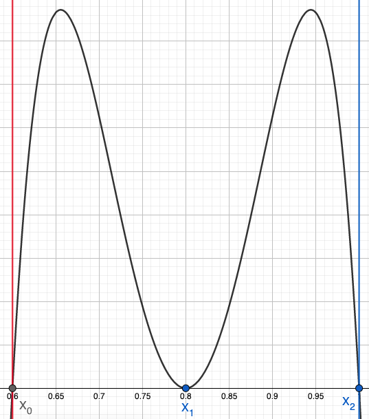
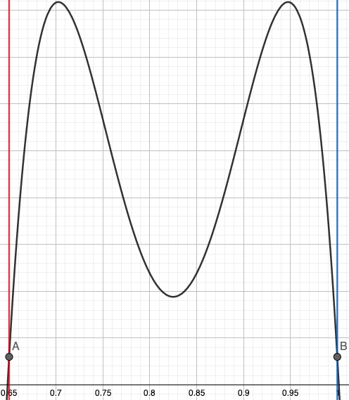
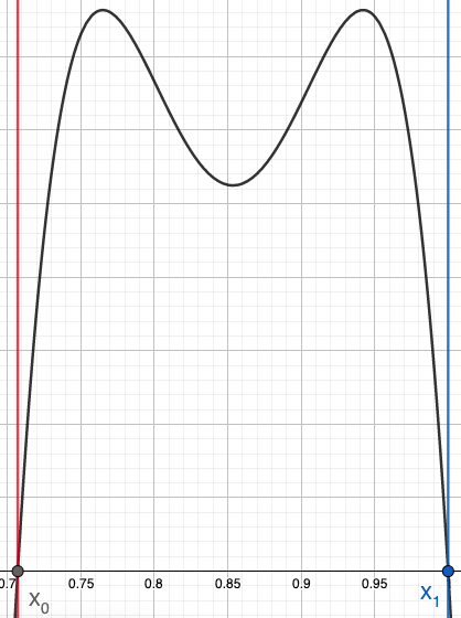
Figure 2. $G_{\kappa=4}^{E}(x)$. $x\in[E-1,1]$. From left to right: $E=\mathcal{E}_{1}$, $E=1.65$, $E=\mathcal{E}_{0}$. $G_{\kappa=4}^{E}(x)>0$ in the middle picture, but not in the other two.

7.2. $n=2$ : $2nd$ band.

$X_{1}=\sqrt{2}/2$. Then we solve $T_{4}(\mathcal{E}_{2}-1)=T_{4}(\mathcal{E}_{2}-\sqrt{2}/2)$ which has 2 solutions $\mathcal{E}_{2}=(2+\sqrt{2}\pm\sqrt{2+4\sqrt{2}})/4$. Using the context, it must be that

(7.2) $$\mathcal{E}_{2}=\frac{2+\sqrt{2}+\sqrt{2+4\sqrt{2}}}{4}\simeq 1.54532.$$

It follows that $X_{2}=\mathcal{E}_{2}-X_{1}=(2-\sqrt{2}+\sqrt{2+4\sqrt{2}})/4$. We suppose $\Sigma=[4,8,12,24]$. The solution to $M\rho=0$ is $[\rho_{4},\rho_{8},\rho_{12},\rho_{24}]^{T}\simeq[1,0.81070,0.21647,-0.06593]^{T}$. The function $x\mapsto G_{\kappa}^{E}(x)$ is plotted in Figure 3 for some values $E\in[\mathcal{E}_{2},\mathcal{E}_{1}]$.

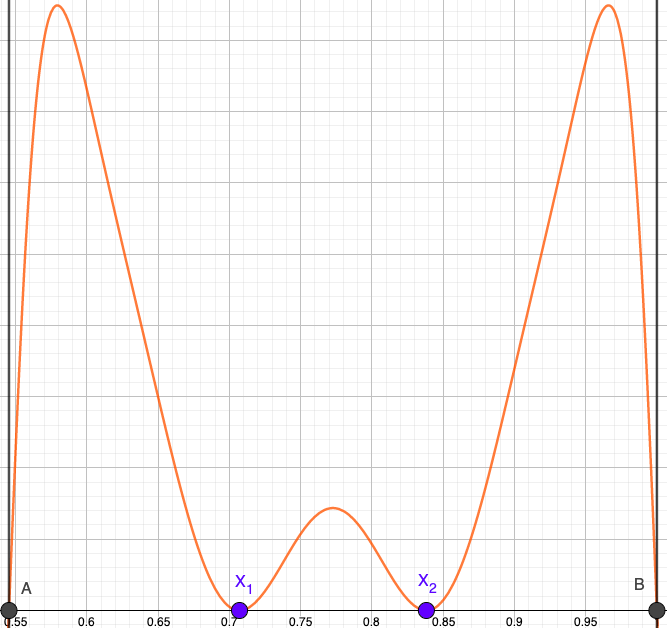
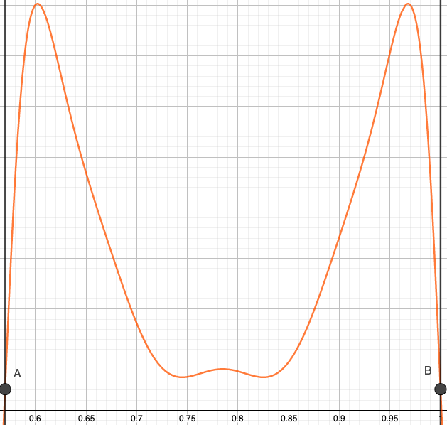
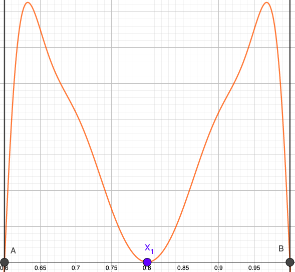
Figure 3. $G_{\kappa=4}^{E}(x)$. $x\in[E-1,1]$. From left to right: $E=\mathcal{E}_{2}$, $E=1.57$, $E=\mathcal{E}_{1}$. $G_{\kappa=4}^{E}(x)>0$ in the middle picture, but not in the other two.

Moreover it would appear that the combinations $\Sigma=[4,8,12,28],[4,8,12,32],[4,8,16,24]$ are equally valid, whereas $\Sigma=[4,8,12,16],[4,8,12,20],[4,8,16,20]$ are not valid. The linear dependency between rows of $M$ seems to rely (at least partly) on the relations

$$U_{4j-1}(1/\sqrt{2})=0,\quad\text{and}\quad U_{4j-1}(\sqrt{2}/\sqrt{3})=-\sqrt{2}U_{4j-1}(1/\sqrt{3}),\quad j\in\mathbb{N}^{*}.$$

7.3. $n=3$ : $3rd$ band.

$X_{2}=\mathcal{E}_{3}/2$ and $T_{4}(\mathcal{E}_{3}-1)=T_{4}(\mathcal{E}_{3}-X_{1})$, $T_{4}(X_{1})=T_{4}(\mathcal{E}_{3}/2)$. Taking the context into account and applying (7.1) leads to $(\mathcal{E}_{3}-1)^{2}+(\mathcal{E}_{3}-X_{1})^{2}=1$ and $X_{1}^{2}+\mathcal{E}_{3}^{2}/4=1$. So

(7.3) $$\mathcal{E}_{3}=\frac{28}{65}+\frac{2}{65t}+\frac{1}{2}\sqrt{\frac{4256}{12675}+\frac{368}{195s}-\frac{16}{195}s+\frac{121088t}{4225}}\simeq 1.51271,\quad t:=\sqrt{\frac{3}{133-\frac{1495}{s}+65s}}$$

and $s:=(629+48\sqrt{177})^{1/3}$. The minimal polynomial for $\mathcal{E}_{3}$ is $mp(E)=65E^{4}-112E^{3}+56E^{2}-64E+16$. Also $X_{1}\simeq 0.65415$, $X_{2}\simeq 0.75635$. We choose the combination $\Sigma=[4,8,12,16,24,36]$. The solution to $M\rho=0$ is

$$[\rho_{4},\rho_{8},\rho_{12},\rho_{16},\rho_{24},\rho_{36}]^{T}\simeq[1,1.18290,0.68875,0.18594,-0.00794,-0.00288]^{T}.$$

The function $G_{\kappa}^{E}(x)$ is plotted in Figure 4 for some values $E\in[\mathcal{E}_{3},\mathcal{E}_{2}]$. The linear dependency between rows of $M$ seems to rely (at least partly) on the relation

$$\left[U_{4j-1}(x),U_{4l-1}\left(\sqrt{1-x^{2}}\right)\right]=0,\quad\forall j,l\in\mathbb{N}^{*},$$

where $[\cdot,\cdot]$ is the Bezoutian defined by [GM3, (2.3) of section 2].

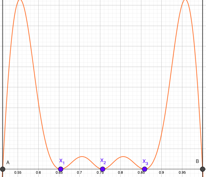
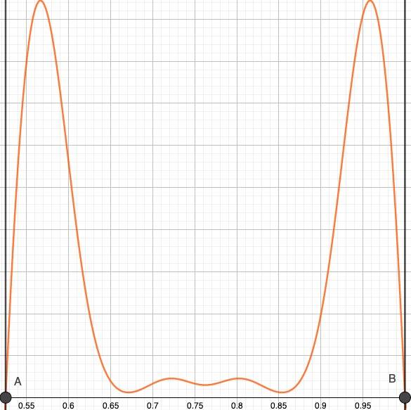
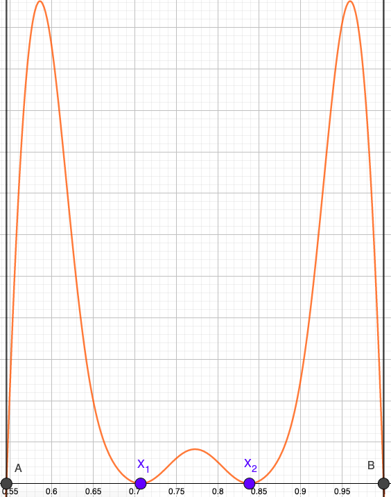
Figure 4. $G_{\kappa=4}^{E}(x)$. $x\in[E-1,1]$. From left to right: $E=\mathcal{E}_{3}$, $E=1.525$, $E=\mathcal{E}_{2}$. $G_{\kappa=4}^{E}(x)>0$ in the middle picture, but not in the other two.

The combination $\Sigma=[4,8,12,16,20,24]$ is equally valid and it gives

$$[\rho_{4},\rho_{8},\rho_{12},\rho_{16},\rho_{20},\rho_{24}]^{T}\simeq[1,1.37002,1.06973,0.53992,0.16964,0.02655]^{T}.$$

7.4. $n=4$ : $4th$ band.

$X_{2}=\sqrt{2}/2$. Then we have to solve $(\mathcal{E}_{4}-1)^{2}+(\mathcal{E}_{4}-X_{1})^{2}=1$, $X_{1}^{2}+(\mathcal{E}_{4}-\sqrt{2}/2)^{2}=1$. This leads to $1-(\mathcal{E}_{4}-\sqrt{2}/2)^{2}=(\mathcal{E}_{4}-\sqrt{\mathcal{E}_{4}(2-\mathcal{E}_{4})})^{2}$. Thus $\mathcal{E}_{4}$ is the root of

$$mp(E)=5E^{4}-(2\sqrt{2}+4)E^{3}+(5-4\sqrt{2})E^{2}+(\sqrt{2}-2)E+1/4=0.$$

The closed form formula of $\mathcal{E}_{4}$ is horrendous; but $\mathcal{E}_{4}\simeq 1.49137$. In turn, $X_{1}\simeq 0.62042$.

The simplest valid combination of indices we have found is $\Sigma=[4,8,12,16,20,24,28,52]$. The solution to $M\rho=0$ is $\rho=[\rho_{4},\rho_{8},\rho_{12},\rho_{16},\rho_{20},\rho_{24},\rho_{28},\rho_{52}]^{T}\simeq$

$$[1,1.46864,1.29941,0.80098,0.34657,0.09808,0.01417,0.000030]^{T}.$$

Graphically $x\mapsto G_{\kappa}^{E}(x)$ is strictly positive for $E\in(\mathcal{E}_{4},\mathcal{E}_{3})$, $x\in[E-1,1]$.

7.5. $n=5$ : $5th$ band.

We have $X_{3}=\mathcal{E}_{5}/2$, $(\mathcal{E}_{5}-1)^{2}+(\mathcal{E}_{5}-X_{1})^{2}=1$, $X_{1}^{2}+(\mathcal{E}_{5}-X_{2})^{2}=1$, and $X_{2}^{2}+(\mathcal{E}_{5}/2)^{2}=1$. This leads to $1-\left(\mathcal{E}_{5}-\left(1-\mathcal{E}_{5}^{2}/4\right)^{1/2}\right)^{2}=\left(\mathcal{E}_{5}-\mathcal{E}_{5}^{1/2}(2-\mathcal{E}_{5})^{1/2}\right)^{2}.$ The solution is

(7.4) $$\mathcal{E}_{5}=\frac{16}{1275}\left(42+\frac{w}{3^{2/3}}-\frac{32533w^{-1}}{3^{1/3}}\right)\simeq 1.47650,\quad w:=(13025367+208250\sqrt{6294})^{1/3}$$

and its minimal polynomial is $mp(E)=-32768+22784E-6048E^{2}+3825E^{3}.$ In turn $X_{1}\simeq 0.59734$, $X_{2}\simeq 0.67452$, $X_{3}\simeq 0.73825$, $X_{4}\simeq 0.80198$ and $X_{5}\simeq 0.87916$. We choose $\Sigma=[4,8,12,16,20,24,28,32,36,40]$. $M\rho=0$ gives $[\rho_{4},\rho_{8},\rho_{12},\rho_{16},\rho_{20},\rho_{24},\rho_{28},\rho_{32},\rho_{36},\rho_{40}]^{T}\simeq$

$$[1,1.58691,1.60962,1.22543,0.72779,0.33759,0.11956,0.03071,0.00514,0.00042]^{T}.$$

It appears graphically that $x\mapsto G_{\kappa}^{E}(x)$ is strictly positive for $E\in(\mathcal{E}_{5},\mathcal{E}_{4})$, $x\in[E-1,1]$.

7.6. $n=6$ : $6th$ band.

$X_{3}=\sqrt{2}/2$, $(\mathcal{E}_{6}-1)^{2}+(\mathcal{E}_{6}-X_{1})^{2}=1$, $X_{1}^{2}+(\mathcal{E}_{6}-X_{2})^{2}=1$ and $X_{2}^{2}+(\mathcal{E}_{6}-\sqrt{2}/2)^{2}=1$. Performing elementary operations shows that $\mathcal{E}_{6}\simeq 1.46568$ is a root of the polynomial

$$mp(E)=384E^{6}+(-448-224\sqrt{2})E^{5}+(200+128\sqrt{2})E^{4}+(-72-52\sqrt{2})E^{3}+(16+12\sqrt{2})E^{2}+(-2-\sqrt{2})E+1/8.$$

In turn $X_{1}\simeq 0.58072$, $X_{2}\simeq 0.65158$, $X_{3}\simeq 0.70710$, $X_{4}\simeq 0.75857$, $X_{5}\simeq 0.81409$, $X_{6}\simeq 0.88495$.

8. Application of Polynomial Interpolation for the first band ($n=1$), $2\leq\kappa\leq 9$

This section is about the first band ($n=1$) in the interval $J_{2}(\kappa)$. For the $1st$ band we suppose only 2 terms in the linear combination [GM3, (1.6) of Introduction] are required. In other words, we suppose $\Sigma=[j_{1}\kappa,j_{2}\kappa]$. According to [GM3, section 12] we look to solve the system

(8.1) $$\begin{cases}g_{j_{1}\kappa}^{\mathcal{E}_{1}}(x)+\rho_{j_{2}\kappa}\cdot g^{\mathcal{E}_{1}}_{j_{2}\kappa}(x)=0,&\text{at}\ x=X_{0}=\mathcal{E}_{1}-1,\\[3.00003pt] g^{\mathcal{E}_{1}}_{j_{1}\kappa}(x)+\rho_{j_{2}\kappa}\cdot g^{\mathcal{E}_{1}}_{j_{2}\kappa}(x)=0,&\text{at}\ x=X_{1},\\[3.00003pt] \frac{d}{dx}g^{\mathcal{E}_{1}}_{j_{1}\kappa}(x)+\rho_{j_{2}\kappa}\cdot\frac{d}{dx}g^{\mathcal{E}_{1}}_{j_{2}\kappa}(x)=0,&\text{at}\ x=X_{1},\\[3.00003pt] g^{\mathcal{E}_{0}}_{j_{1}\kappa}(x)+\rho_{j_{2}\kappa}\cdot g^{\mathcal{E}_{0}}_{j_{2}\kappa}(x)=0,&\text{at}\ \mathcal{E}_{0}=1+\cos(\pi/\kappa),x=\mathcal{E}_{0}-1.\end{cases}$$

Note we are assuming $\rho_{j_{1}\kappa}=1$. By [GM3, Remark 5.2], $X_{1}=\mathcal{E}_{1}/2$. So the $3rd$ line of (8.1) is trivially true, by [GM3, Lemma 3.4]. The $4th$ line is also always true, by [GM3, Lemma 1.4]. Assuming $\mathcal{E}_{1}\neq 0,\pm 2$, the system (8.1) is equivalent to

(8.2) $$\begin{cases}[U_{j_{1}\kappa-1}(\mathcal{E}_{1}-1),U_{j_{2}\kappa-1}(\mathcal{E}_{1}/2)]=0,\\ X_{1}=\mathcal{E}_{1}/2,\\ \rho_{j_{2}\kappa}=-U_{j_{1}\kappa-1}(\mathcal{E}_{1}-1)/U_{j_{2}\kappa-1}(\mathcal{E}_{1}-1)=-U_{j_{1}\kappa-1}(\mathcal{E}_{1}/2)/U_{j_{2}\kappa-1}(\mathcal{E}_{1}/2).\end{cases}$$

Let $X_{2}:=1$, $X_{0}=\mathcal{E}_{1}-X_{2}=\mathcal{E}_{1}-1$. From the $3rd$ line of (8.2) we see that we want $U_{j\kappa-1}(X_{0})\neq 0$ and $U_{j\kappa-1}(X_{1})\neq 0$, in particular $U_{\kappa-1}(X_{0}),U_{\kappa-1}(X_{1})\neq 0$. Thus, by [GM3, Corollary 2.3] we see that (8.2) is equivalent to

(8.3) $$\begin{cases}X_{2}=1,\\ X_{0}=\mathcal{E}_{1}-X_{2},\\ X_{1}=\mathcal{E}_{1}/2,\\ T_{\kappa}(X_{0})=T_{\kappa}(X_{1}),\\ \rho_{j_{2}\kappa}=-U_{j_{1}\kappa-1}(\mathcal{E}_{1}-1)/U_{j_{2}\kappa-1}(\mathcal{E}_{1}-1)=-U_{j_{1}\kappa-1}(\mathcal{E}_{1}/2)/U_{j_{2}\kappa-1}(\mathcal{E}_{1}/2).\end{cases}$$

This is in agreement with [GM3, (5.1) of section 5] for $n=1$. In practice, our assessment is that it is best to simply take $\Sigma=\{j_{1}\kappa,j_{2}\kappa\}=\{\kappa,2\kappa\}$. Table 3 lists the results for $\kappa\in\{2,...,9\}$.

$\kappa$	Solution to (8.3)	$\kappa$	Solution to (8.3)
2	$\mathcal{E}_{1}=\frac{2}{3}$	3	$\mathcal{E}_{1}=\frac{5+3\sqrt{2}}{7}\simeq 1.3203$
2	$\rho_{4}=\frac{9}{14}\simeq 0.6428$	3	$\rho_{6}=\frac{170-81\sqrt{2}}{92}\simeq 0.6027$
4	$\mathcal{E}_{1}=\frac{8}{5}$	5	$\mathcal{E}_{1}=\frac{49+12\sqrt{10}+\sqrt{5(49+12\sqrt{10})}}{62}\simeq 1.7386$
4	$\rho_{8}=\frac{625}{1054}\simeq 0.5929$	5	$\rho_{10}=\frac{-4000073+2667375\sqrt{2}+225\sqrt{5(25786331-6299370\sqrt{2})}}{3122396}\simeq 0.5889$
6	$\mathcal{E}_{1}=1+\sqrt{\frac{2}{3}}\simeq 1.8164$	7	$\mathcal{E}_{1}\simeq 1.8642$ (closed form unknown to us)
6	$\rho_{12}=\frac{27}{46}\simeq 0.5869$	7	$\rho_{14}\simeq 0.5857$
8	$\mathcal{E}_{1}=\frac{16+3\sqrt{2}+2\sqrt{26+7\sqrt{2}}}{17}$	9	$\mathcal{E}_{1}\simeq 1.9173$ (closed form unknown to us)
8	$\mathcal{E}_{1}\simeq 1.8956$
8	$\rho_{16}\simeq 0.5850$	9	$\rho_{18}\simeq 0.5844$

Table 3. Solutions to (8.3). $\mathcal{E}_{1}=1st$ band’s left endpoint.

9. Energy thresholds in $(0,1/2)$ for $\kappa=3$ in dimension 2

Fix $\kappa=3$, in dimension 2. We construct graphically a bunch of thresholds in $(0,1/2)$. Recall that by [GM3, Lemma 5.3], $\mathfrak{T}_{n,\kappa}=-\mathfrak{T}_{n,\kappa}$, or by [GM3, Lemma 3.2], $\bm{\Theta}_{\kappa}(\Delta)=-\bm{\Theta}_{\kappa}(\Delta)$. So the negative thresholds listed below have a positive counterpart.

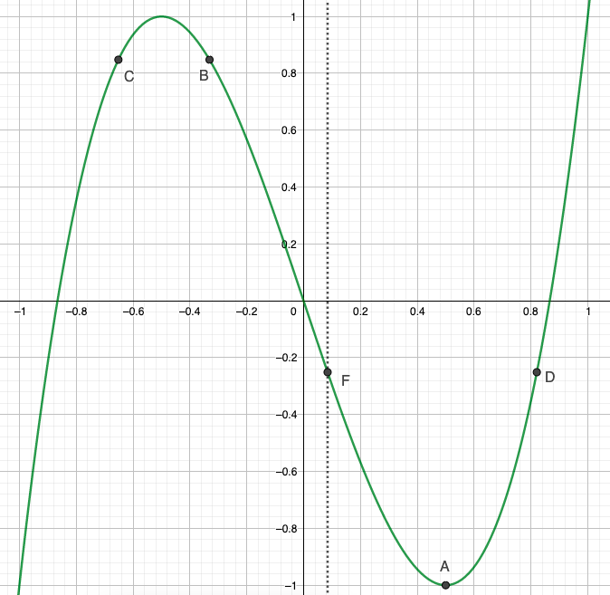
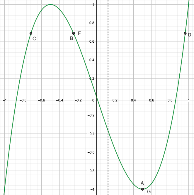
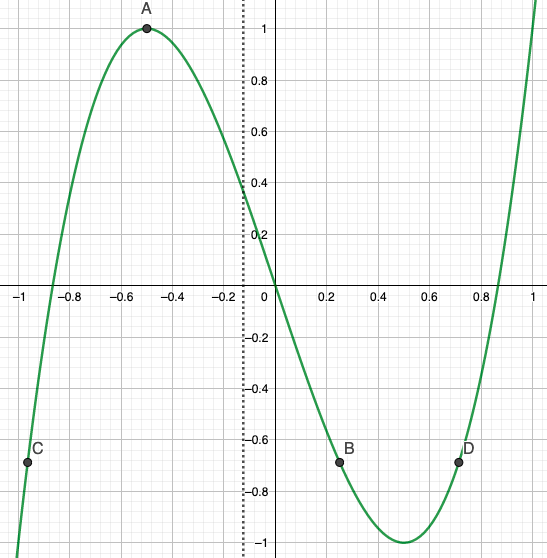
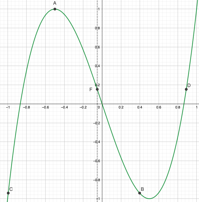
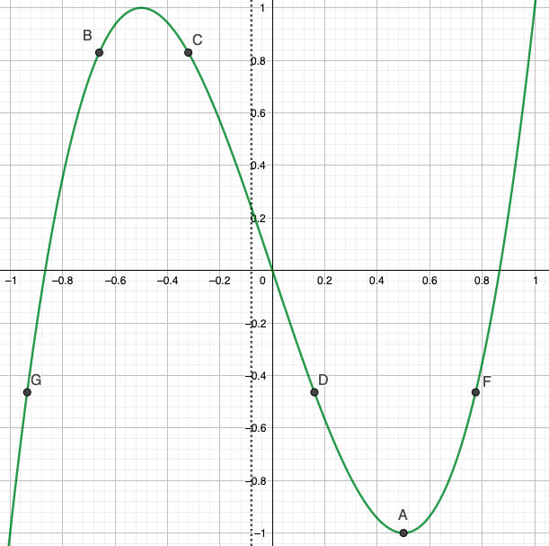
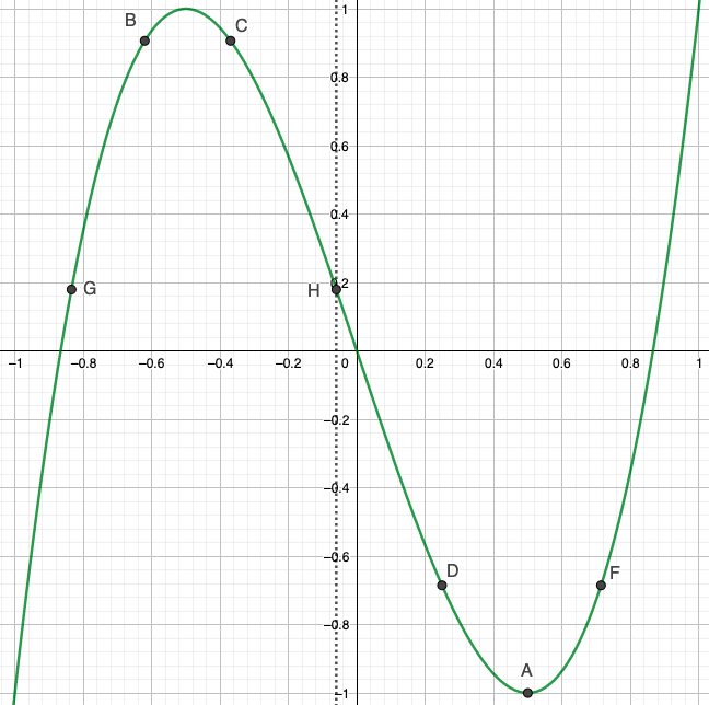
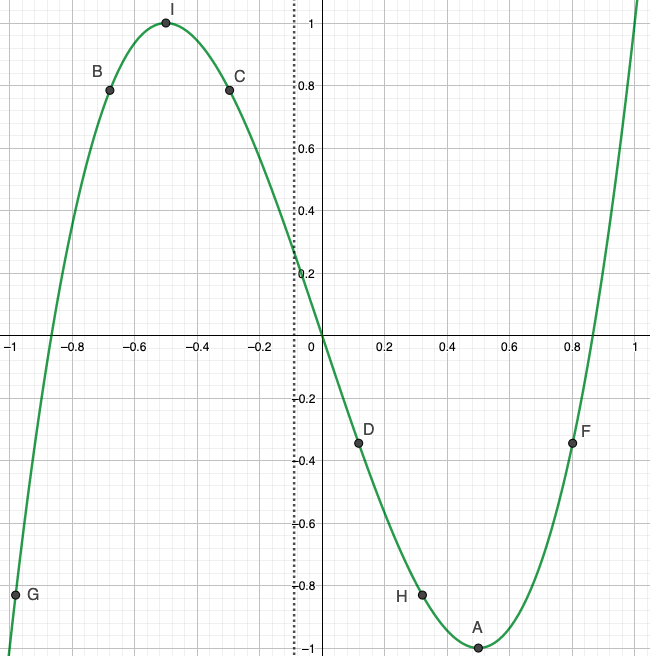
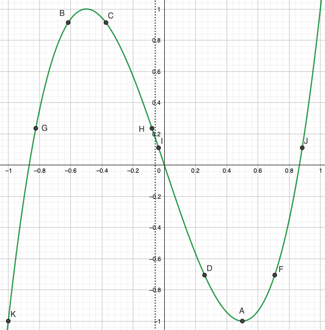
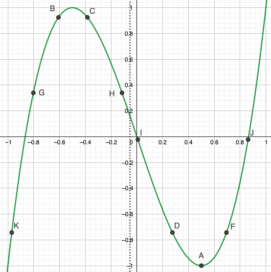
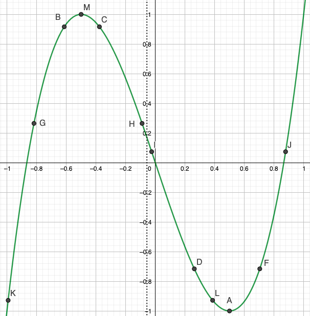
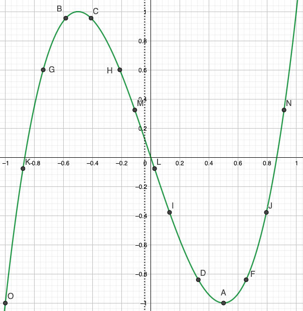
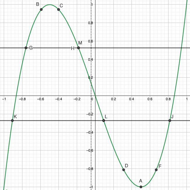
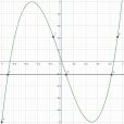
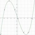
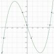
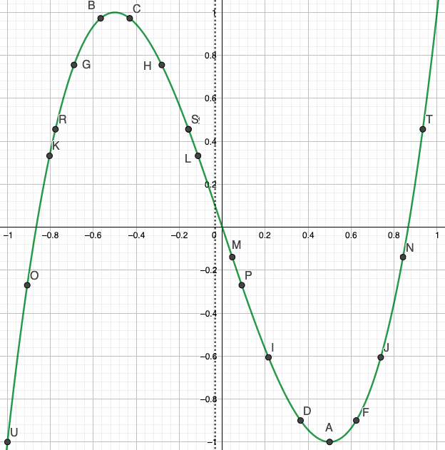
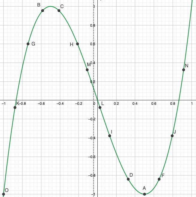
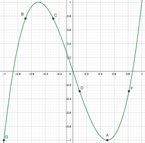
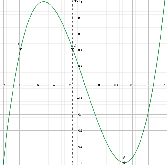
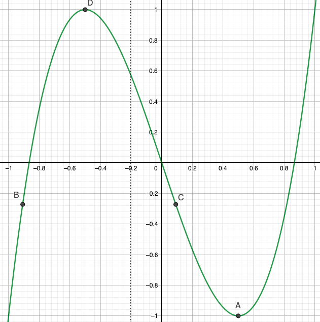
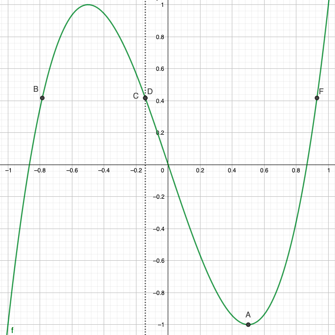
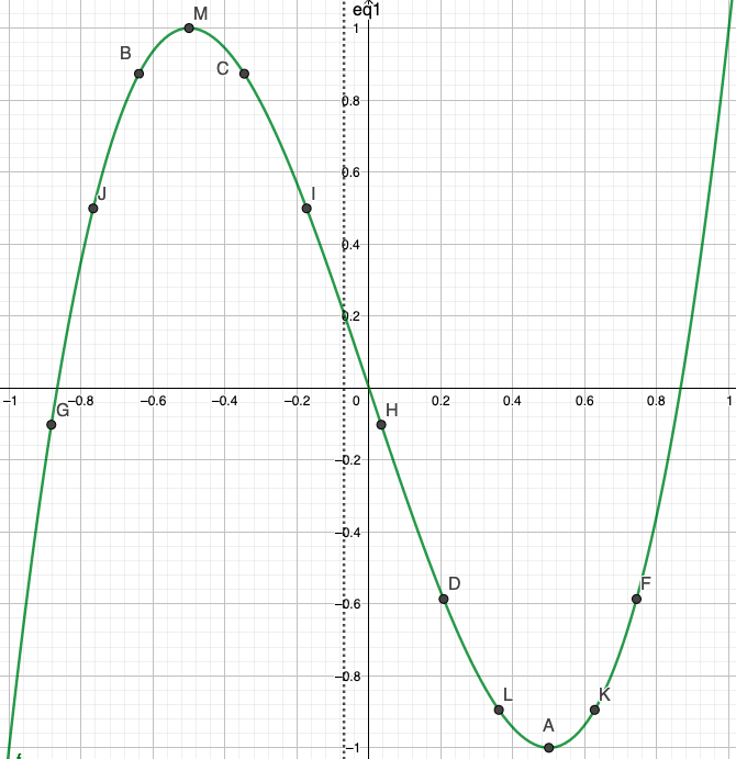
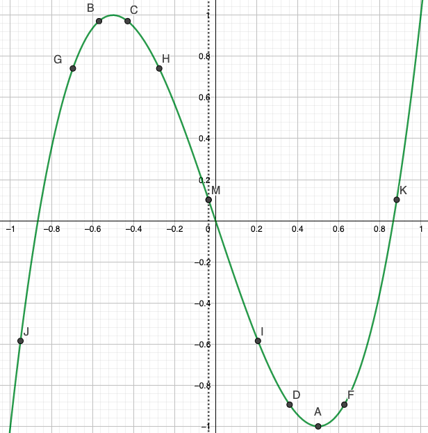
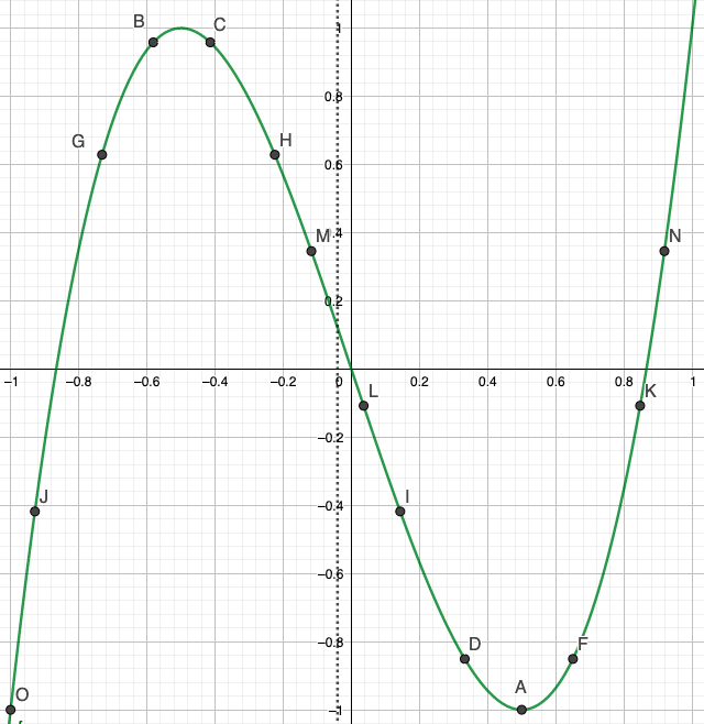
Figure 5.

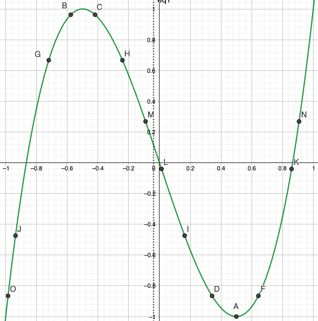
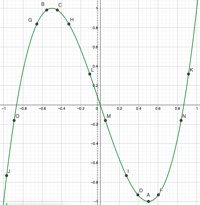
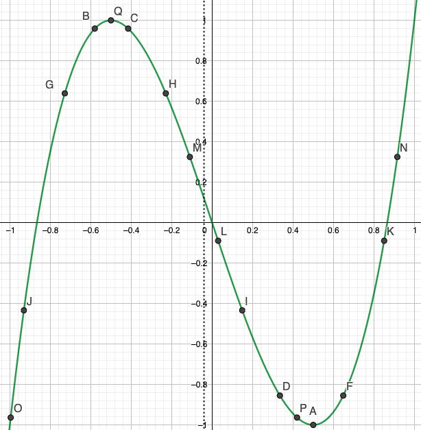
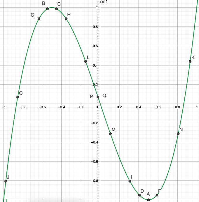
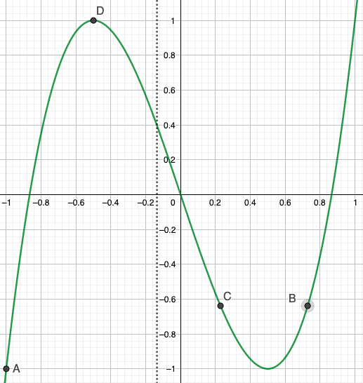
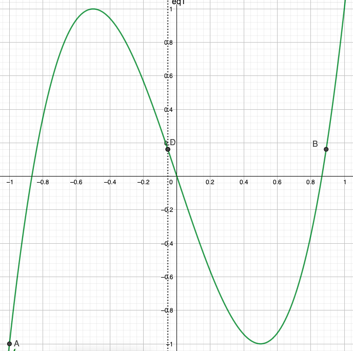
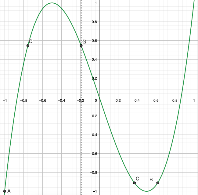
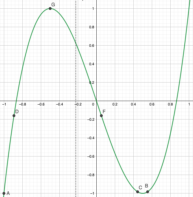
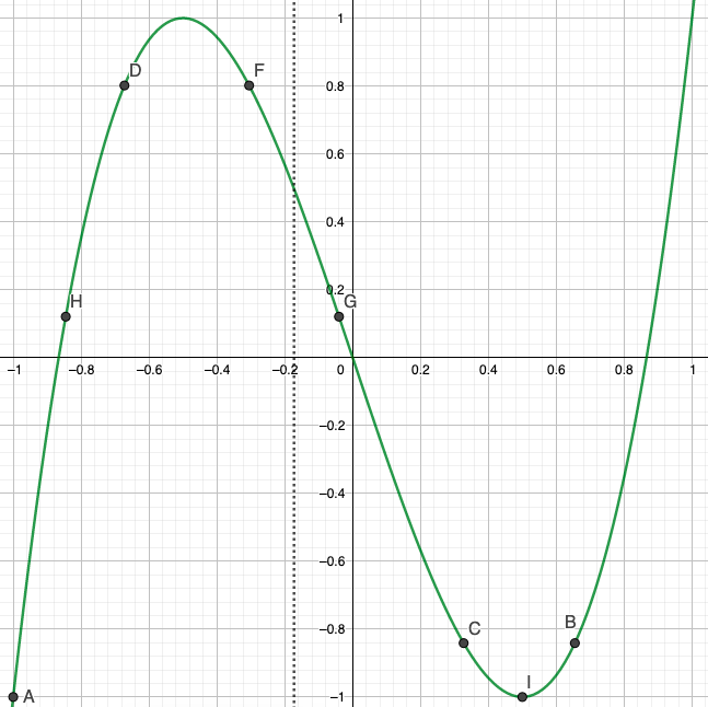
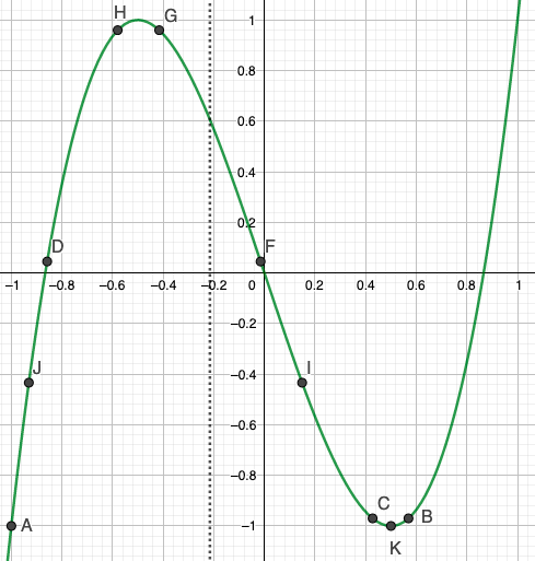
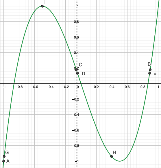
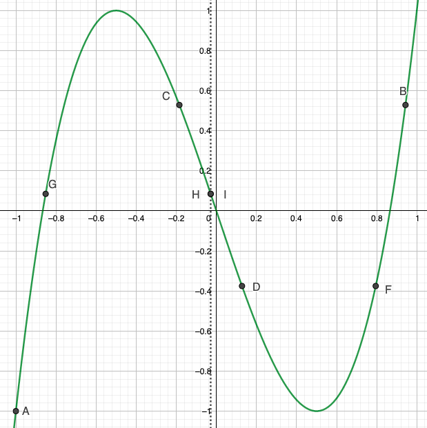
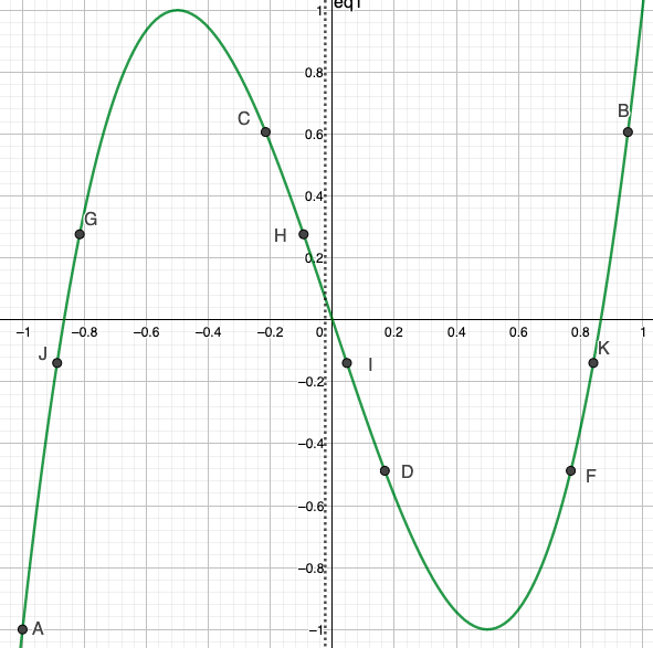
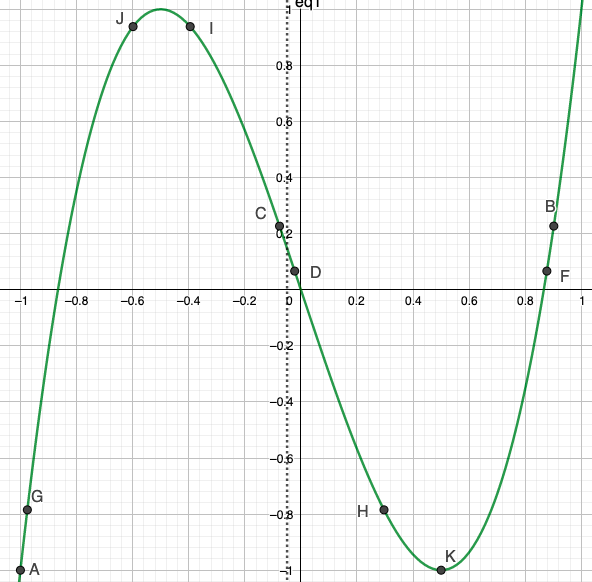
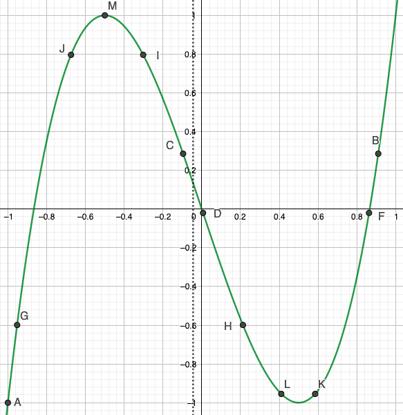
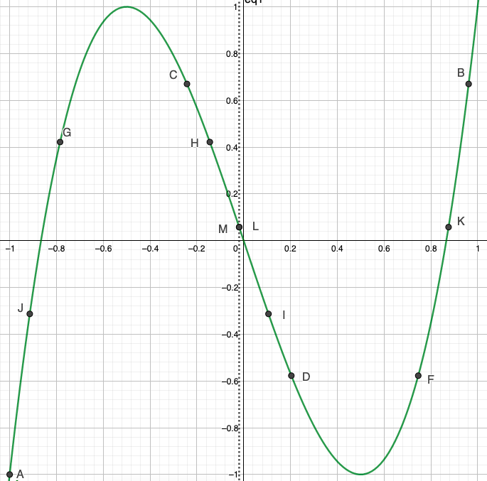
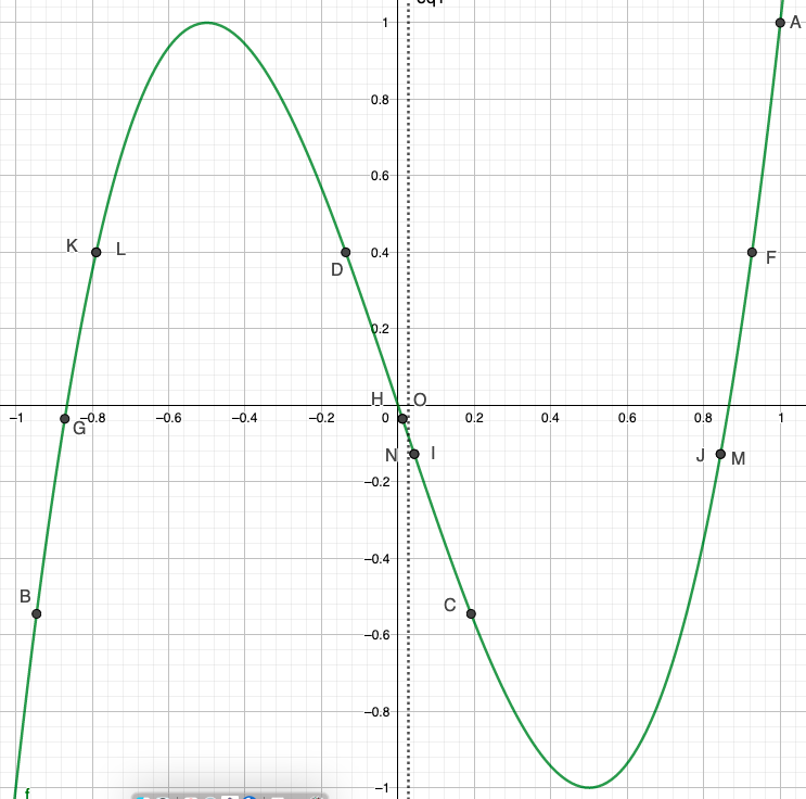
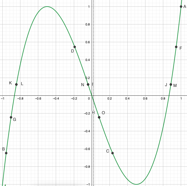
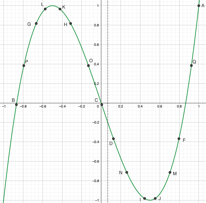
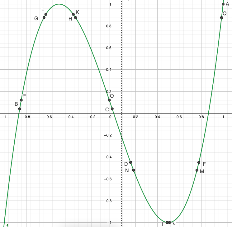
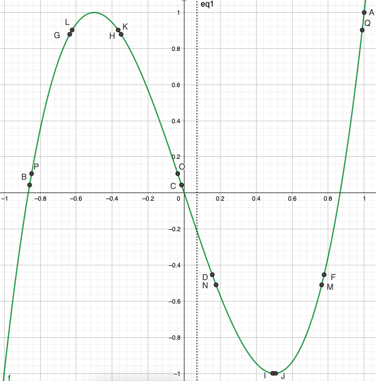
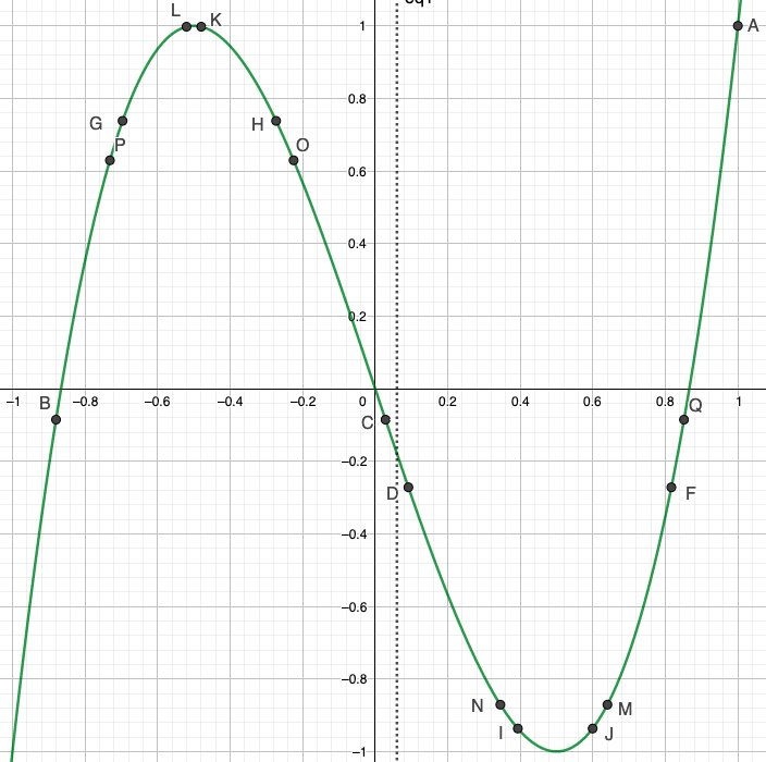
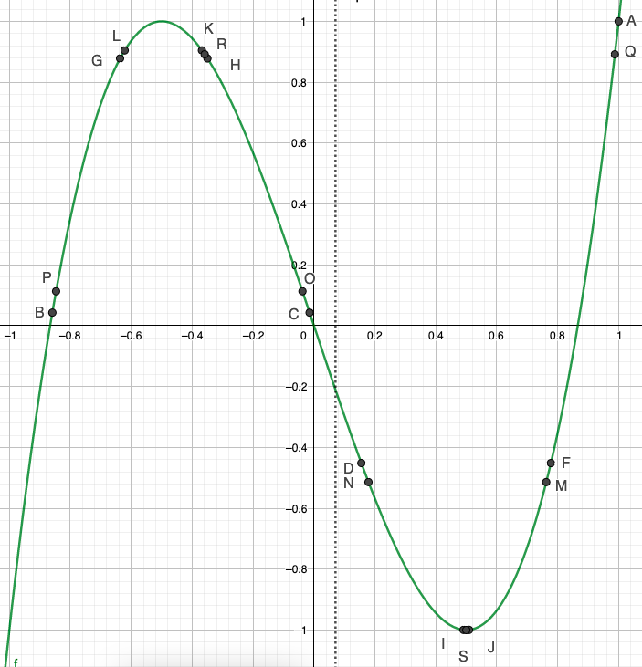
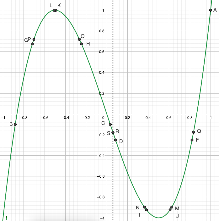
Figure 6.

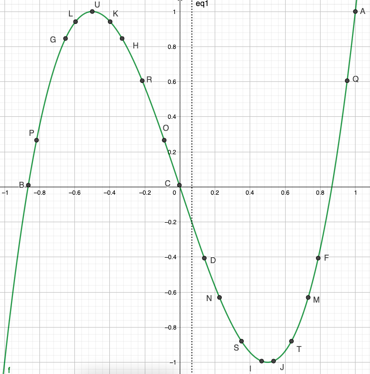
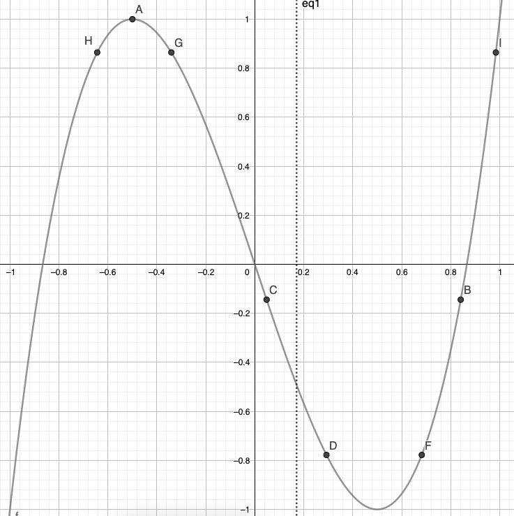
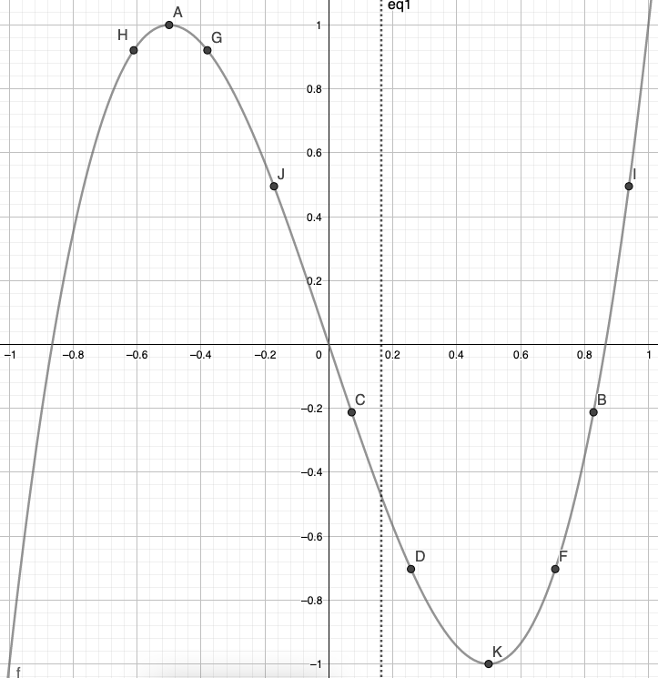
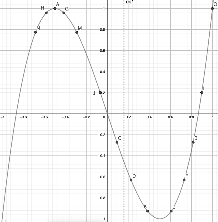
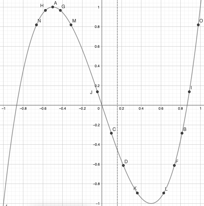
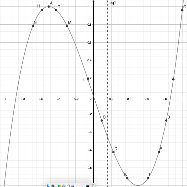
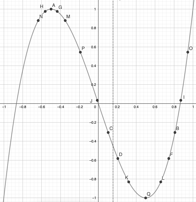
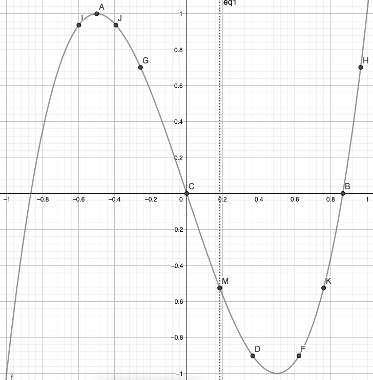
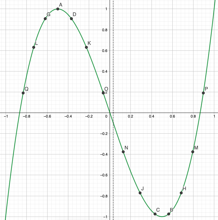
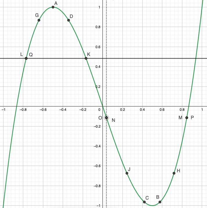
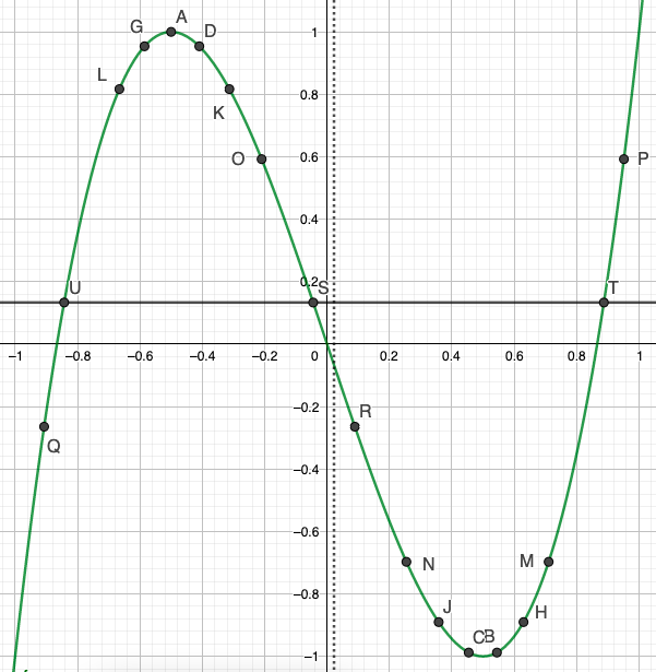
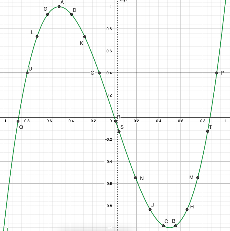
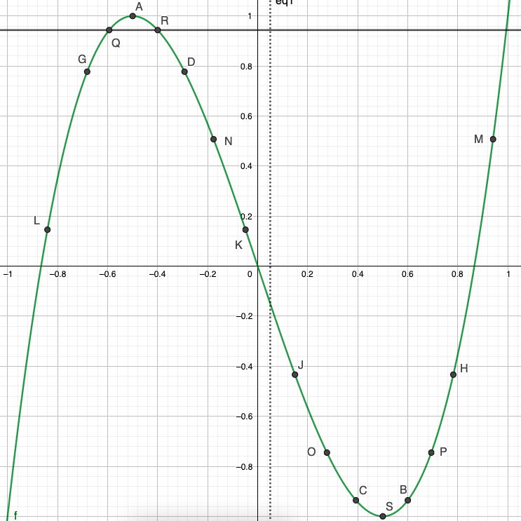
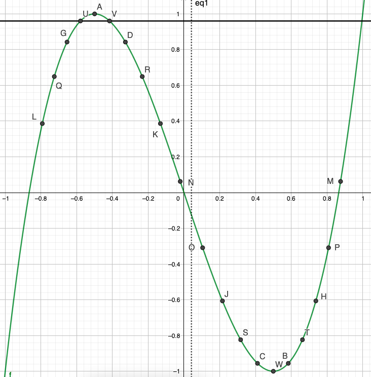
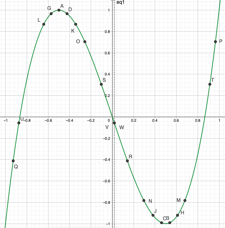
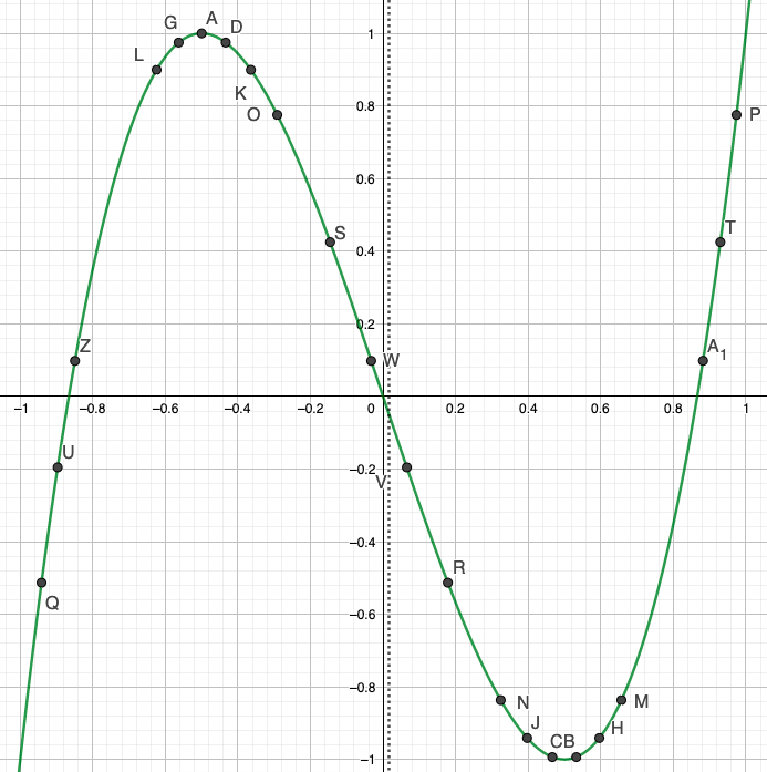
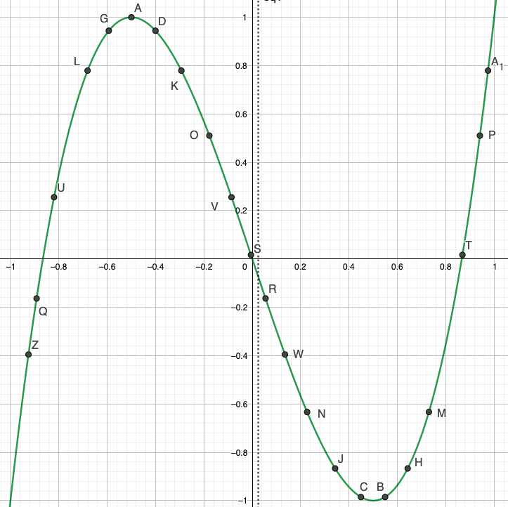
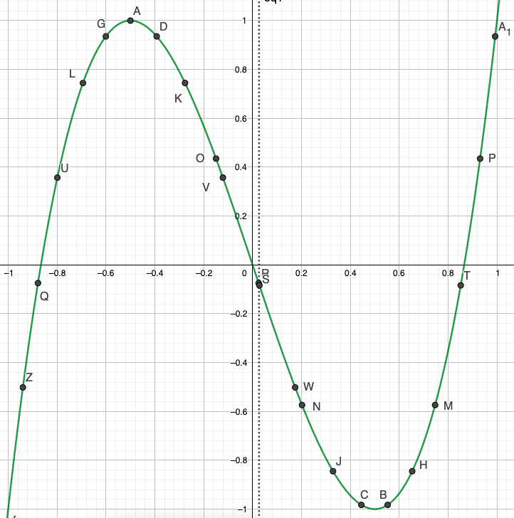
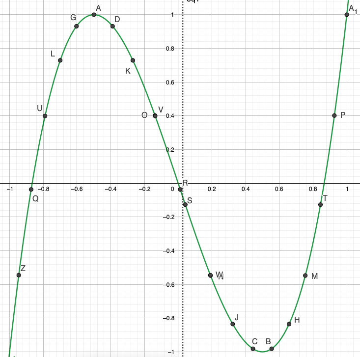
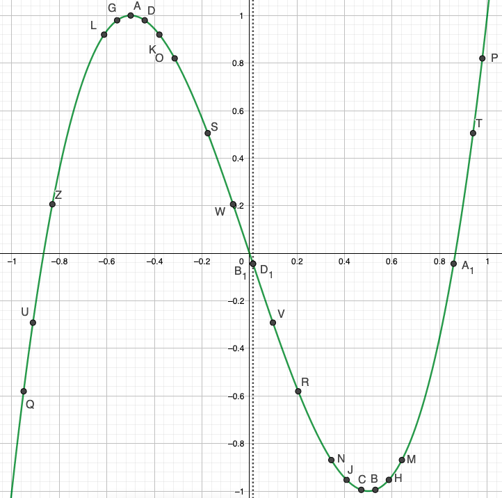
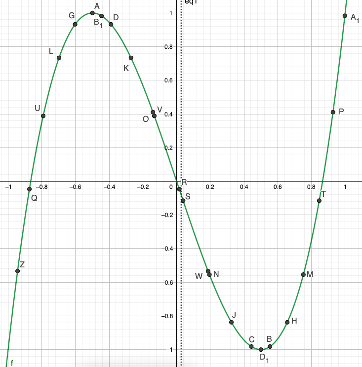
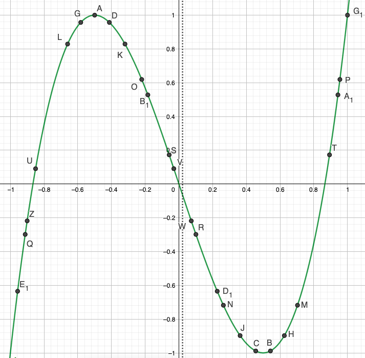
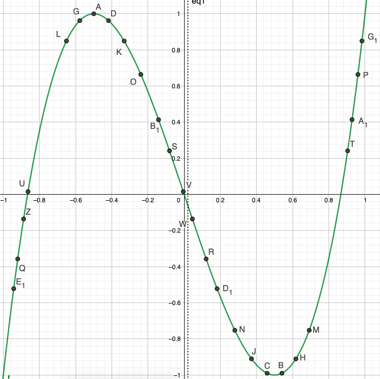
Figure 7.

1) $\mathcal{E}\simeq 0.169$.

2) $\mathcal{E}=0.25$.

3) $\mathcal{E}=-0.25$.

4) $\mathcal{E}\simeq-0.1028$.

5) $\mathcal{E}\simeq-0.16019$.

6) $\mathcal{E}\simeq-0.1202$.

7) $\mathcal{E}\simeq-0.17911$.

8) $\mathcal{E}\simeq-0.11608$.

9) $\mathcal{E}\simeq-0.10796$.

10) $\mathcal{E}\simeq-0.11385$.

11) $\mathcal{E}\simeq-0.08425$.

12) $\mathcal{E}\simeq-0.0917$.

13) $\mathcal{E}\simeq-0.07143$.

14) $\mathcal{E}\simeq-0.14325$.

15) $\mathcal{E}\simeq-0.05169$.

16) $\mathcal{E}\simeq-0.06615$.

17) $\mathcal{E}\simeq-0.08424$.

18) $\mathcal{E}\simeq-0.18726$.

19) $\mathcal{E}\simeq-0.2857$.

20) $\mathcal{E}\simeq-0.40824$.

21) $\mathcal{E}\simeq-0.2857$.

22) $\mathcal{E}\simeq-0.13911$.

23) $\mathcal{E}\simeq-0.06805$.

24) $\mathcal{E}\simeq-0.0813$.

25) $\mathcal{E}\simeq-0.07704$.

26) $\mathcal{E}\simeq-0.05406$.

27) $\mathcal{E}\simeq-0.08014$.

28) $\mathcal{E}\simeq-0.04594$.

29) $\mathcal{E}\simeq-0.27129$.

30) $\mathcal{E}\simeq-0.1082$.

31) $\mathcal{E}\simeq-0.38229$.

32) $\mathcal{E}\simeq-0.4467$.

33) $\mathcal{E}\simeq-0.34518$.

34) $\mathcal{E}\simeq-0.43085$.

35) $\mathcal{E}\simeq-0.105384$.

36) $\mathcal{E}\simeq-0.05659$.

37) $\mathcal{E}\simeq-0.04657$.

38) $\mathcal{E}\simeq-0.09839$.

39) $\mathcal{E}\simeq-0.08979$.

40) $\mathcal{E}\simeq-0.03862$.

41) $\mathcal{E}\simeq+0.05439$.

42) $\mathcal{E}\simeq+0.04135$.

43) $\mathcal{E}\simeq+0.13104$.

44) $\mathcal{E}\simeq+0.14092$.

45) $\mathcal{E}\simeq+0.14142$.

46) $\mathcal{E}\simeq+0.12009$.

47) $\mathcal{E}\simeq+0.14121$.

48) $\mathcal{E}\simeq+0.11771$.

49) $\mathcal{E}\simeq+0.13562$.

50) $\mathcal{E}\simeq+0.34089$.

51) $\mathcal{E}\simeq+0.32821$.

52) $\mathcal{E}\simeq+0.31674$.

53) $\mathcal{E}\simeq+0.31404$.

54) $\mathcal{E}\simeq+0.31616$.

55) $\mathcal{E}\simeq+0.30948$.

56) $\mathcal{E}\simeq+0.36612$.

57) $\mathcal{E}\simeq+0.06397$.

58) $\mathcal{E}\simeq+0.07628$.

59) $\mathcal{E}\simeq+0.04454$.

60) $\mathcal{E}\simeq+0.05450$.

61) $\mathcal{E}\simeq+0.1001$.

62) $\mathcal{E}\simeq+0.08365$.

63) $\mathcal{E}\simeq+0.03773$.

64) $\mathcal{E}\simeq+0.03277$.

65) $\mathcal{E}\simeq+0.04901$.

66) $\mathcal{E}\simeq+0.05283$.

67) $\mathcal{E}\simeq+0.05445$.

68) $\mathcal{E}\simeq+0.02930$.

69) $\mathcal{E}\simeq+0.05402$.

70) $\mathcal{E}\simeq+0.04300$.

71) $\mathcal{E}\simeq+0.04030$.