Thresholds and more bands of A.C. spectrum for the discrete Schrödinger operator with a more general long range condition

Abstract.

We continue the investigation of the existence of absolutely continuous (a.c.) spectrum for the discrete Schrödinger operator $\Delta+V$ on $\ell^{2}(\mathbb{Z}^{d})$, in dimensions $d\geq 2$, for potentials $V$ satisfying the long range condition $n_{i}(V-\tau_{i}^{\kappa}V)(n)=O(\ln^{-q}(|n|))$ for some $q>2$, $\kappa\in\mathbb{N}$, and all $1\leq i\leq d$, as $|n|\to\infty$. $\tau_{i}^{\kappa}V$ is the potential shifted by $\kappa$ units on the $i^{\text{th}}$ coordinate. The difference between this article and [GM2] is that here finite linear combinations of conjugate operators are constructed leading to more bands of a.c. spectrum being observed. The methodology is backed primarily by graphical evidence because the linear combinations are built by numerically implementing a polynomial interpolation. On the other hand an infinitely countable set of thresholds, whose exact definition is given later, is rigorously identified. Our overall conjecture, at least in dimension 2, is that the spectrum of $\Delta+V$ is void of singular continuous spectrum, and consecutive thresholds are endpoints of a band of a.c. spectrum.

1. Introduction

The discrete Schrödinger operators on the lattice $\mathbb{Z}^{d}$ have a long history in modeling quantum phenomena in media with discrete postions such as crystals, or more general media by means of discretisation. This article deals with a specific modeling aspect in the spectral theory of these operators and is a direct sequel to [GM2]. Let $\mathscr{H}:=\ell^{2}(\mathbb{Z}^{d})$. The discrete Laplacian on $\mathbb{Z}^{d}$, which models the kinetic energy of a quantum particle, is

(1.1) $$\Delta=\Delta[d]:=\Delta_{1}+...+\Delta_{d},\quad\text{where }\Delta_{i}:=(S_{i}+S^{*}_{i})/2.$$

Here $S_{i}=S_{i}^{1}$ and $S^{*}_{i}=S^{-1}_{i}$ are the shifts to the right and left respectively on the $i^{th}$ coordinate. So $(S_{i}^{\pm 1}u)(n)=u(n_{1},\ldots,n_{i}\mp 1,\ldots,n_{d})$ for $u\in\mathscr{H}$, $n=(n_{1},\ldots,n_{d})\in\mathbb{Z}^{d}$. Set $|n|^{2}=n_{1}^{2}+...+n_{d}^{2}$. Let $\sigma(\cdot)$ denote the spectrum of an operator. A Fourier transformation shows that the spectra of $\Delta_{i}$ and $\Delta$ are purely absolutely continuous (a.c.), $\sigma(\Delta_{i})\equiv[-1,1]$ and $\sigma(\Delta)=[-d,d]$.

Let $V$ model a discrete electric potential and act pointwise, i.e. $(Vu)(n)=V(n)u(n)$, for $u\in\mathscr{H}$. We always assume $V$ is real-valued and goes to zero at infinity. Thus the essential spectrum of $\Delta+V$ equals $\sigma(\Delta)$. Let $\mathbb{N}$ and $\mathbb{N}^{*}$ be the positive integers, including and excluding zero respectively. Fix $\kappa\in\mathbb{N}^{*}$. The shifted potential by $\pm\kappa$ units is defined by

$$(\tau_{i}^{\pm\kappa}V)u(n):=V(n_{1},\ldots,n_{i}\mp\kappa,\ldots n_{d})u(n),\quad\forall 1\leq i\leq d.$$

As in [GM2], we are interested in potentials $V$ satisfying a non-radial condition of the form

(1.2) $$n_{i}(V-\tau_{i}^{\kappa}V)(n)=O(g(n)),\ \text{as}\ |n|\to\infty,\quad\forall 1\leq i\leq d,$$

where $g(n)$ is a radial function which goes to zero at infinity at an appropriate rate, e.g. $g(n)=\ln^{-q}(|n|+1)$, $q>2$. We refer to [GM2] for some examples of Schrödinger operators that satisfy (1.2). Also, one may generalize (1.2) by shifting $V$ by a different amount in each direction (i.e. $\kappa_{i}$ instead of $\kappa$ in (1.2)). We do not study this question here and refer instead to [GM2] for numerical examples. We also want to mention that the class of $V$ given by (1.2) is quite close to the $V(n)=O(1/|n|)$ class, for which the absence of singular continuous (s.c.) spectrum is proved in dimension 1, see [Li1] and [Ki], but remains an open problem in higher dimensions. In our opinion the transition of spectral components at the $V(n)=O(1/|n|)$ level is still not very well understood, especially in dimensions $\geq 2$, but see e.g. [Li1] and [Li2] for $d=1$. This article may be viewed as a contribution in this direction.

For a closed interval $I\subset\mathbb{R}$ let $I_{\pm}:=\{z\in\mathbb{C}_{\pm}:\mathrm{Re}(z)\in I\}$, $\mathbb{C}_{\pm}:=\{z\in\mathbb{C},\pm\mathrm{Im}(z)>0\}$. The limiting absorption principle (LAP) is a statement about the extension of the holomorphic maps

(1.3) $$I_{\pm}\ni z\mapsto(\Delta+V-z)^{-1}$$

to $I$. The LAP on an interval $I$ implies amongst other things the absence of s.c. spectrum for $\Delta+V$ on that set. This article aims for such type of results. In Mourre theory, which has its origins in [Mo1] and [Mo2], and is extensively refined in [ABG], the strategy to obtain a LAP (1.3) on an interval $I\subset\sigma(\Delta+V)$ depends roughly on the ability to prove two key estimates. The first estimate is a strict Mourre estimate for $\Delta$ with respect to some self-adjoint conjugate operator $\mathbb{A}$ on this interval, that is to say, $\exists\gamma>0$ such that

(1.4) $$1_{I}(\Delta)[\Delta,\mathrm{i}\mathbb{A}]_{\circ}1_{I}(\Delta)\geq\gamma 1_{I}(\Delta),$$

where $1_{I}(\Delta)$ is the spectral projection of $\Delta$ on $I$, and $[\cdot,\mathrm{i}\mathbb{A}]_{\circ}$ initially defined on the compactly supported sequences is the extension of the commutator between two operators to a bounded operator on $\mathscr{H}$ (this definition suffices for this article). The second estimate is one involving $V$, and according to a later version of the theory, is such as

(1.5) $$\ln^{p}(1+|n|)\cdot[V,\mathrm{i}\mathbb{A}]_{\circ}\cdot\ln^{p}(1+|n|)\quad is\ a\ compact\ operator\ on\ \mathscr{H}\ for\ some\ p>1.$$

To specify our choice of $\mathbb{A}$ we need the position operators $(N_{i}u)(n):=n_{i}u(n)$. To handle condition (1.2) we consider a (finite) linear combination of conjugate operators of the form

(1.6) $$\mathbb{A}=\sum_{j\geq 1}\rho_{j\kappa}\cdot A_{j\kappa},\quad\rho_{j\kappa}\in\mathbb{R},\quad A_{j\kappa}:=\sum_{1\leq i\leq d}A_{i}(j,\kappa),$$

where each $A_{i}(j,\kappa)$, initially defined on compactly supported sequences, is the closure in $\mathscr{H}$ of :

(1.7) $$A_{i}(j,\kappa):=\frac{1}{2\mathrm{i}}\bigg{[}\frac{j\kappa}{2}(S_{i}^{j\kappa}+S_{i}^{-j\kappa})+(S_{i}^{j\kappa}-S_{i}^{-j\kappa})N_{i}\bigg{]}=\frac{1}{4\mathrm{i}}\bigg{[}(S_{i}^{j\kappa}-S_{i}^{-j\kappa})N_{i}+N_{i}(S_{i}^{j\kappa}-S_{i}^{-j\kappa})\bigg{]}.$$

Each $A_{j\kappa}$ is self-adjoint in $\mathscr{H}$ by an adaptation of the case $(j,\kappa)=(1,1)$, and so $\mathbb{A}$ is self-adjoint, at least whenever it is a finite sum. The reason choice (1.6) is relevant is that

$$[V,\mathrm{i}A_{j\kappa}]_{\circ}=\sum_{1\leq i\leq d}(4\mathrm{i})^{-1}\left((V-\tau_{i}^{j\kappa}V)S_{i}^{j\kappa}-(V-\tau_{i}^{-j\kappa}V)S_{i}^{-j\kappa}\right)N_{i}+\text{hermitian conjugate},$$

and so (1.2) implies (1.5), again, at least when $\mathbb{A}$ is a finite sum and $g(n)=\ln^{-q}(1+|n|)$, $q>2$. The frequencies of the $A_{i}(j,\kappa)$ are in sync with the long range frequency decay of $V$. But the coefficients $\rho_{j\kappa}$ need to be chosen so that (1.4) holds. This is a challenge. Categorize energies into two sets : $\bm{\mu}_{\kappa}(\Delta)$ and $\bm{\Theta}_{\kappa}(\Delta)$. $\bm{\mu}_{\kappa}(\Delta)$ are energies $E\in\sigma(\Delta)$ for which there is a self-adjoint linear combination (finite or infinite) of the form (1.6), an interval $I\ni E$ and $\gamma>0$ such that the Mourre estimate (1.4) holds. $\bm{\Theta}_{\kappa}(\Delta)$ are energies $E\in\sigma(\Delta)$ for which there is no self-adoint linear combination (finite or infinite) of the form (1.6), no interval $I\ni E$ and no $\gamma>0$ such that (1.4) holds. By definition $\sigma(\Delta)$ is a disjoint union of $\bm{\mu}_{\kappa}(\Delta)$ and $\bm{\Theta}_{\kappa}(\Delta)$. From Mourre theory $\bm{\mu}_{\kappa}(\Delta)$ is an open set and so $\bm{\Theta}_{\kappa}(\Delta)$ is closed. In this article, including title and abstract, we refer to energies in $\bm{\Theta}_{\kappa}(\Delta)$ as thresholds. This definition depends on the modeling assumption of $\mathbb{A}$ (see end of introduction for a comment). To be clear, the family $\mathbb{A}$ given by (1.6) is a modeling assumption within the larger modeling framework of discrete Schrödinger operators given by (1.1). Theorem 1.1 below highlights the usefulness of the sets $\bm{\mu}_{\kappa}(\Delta)$. Let $\sigma_{p}(\Delta+V)$ be the point spectrum of $\Delta+V$. Let $\langle\mathbb{A}\rangle:=\sqrt{1+\mathbb{A}^{*}\mathbb{A}}$.

Theorem 1.1.

Let $q>2$, $\kappa\in\mathbb{N}^{*}$ be such that $\limsup\left(|V(n)|,|n_{i}(V-\tau_{i}^{\kappa}V)(n)|\right)=O\left(\ln^{-q}(|n|)\right)$, as $|n|\to\infty$ and $\forall 1\leq i\leq d$. Let $E\in\bm{\mu}_{\kappa}(\Delta)\setminus\sigma_{p}(\Delta+V)$. Let $\mathbb{A}=\sum_{j}\rho_{j\kappa}A_{j\kappa}$ be a finite sum such that (1.4) holds in a neighorhood of $E$. Then there is an open interval $I$, $I\ni E$, such that

1. $\sigma_{p}(\Delta+V)\cap I$ is at most finite (including multiplicity),

2. $\forall p>1/2$ the map $I_{\pm}\ni z\mapsto(\Delta+V-z)^{-1}\in\mathscr{B}\left(\mathcal{K},\mathcal{K}^{*}\right)$ extends to a uniformly bounded map on $I$, with $\mathcal{K}=L^{2}_{1/2,p}(\mathbb{A})=\left\{\psi\in\mathscr{H}:\|\langle\mathbb{A}\rangle^{1/2}\ln^{p}(\langle\mathbb{A}\rangle)\psi\|<\infty\right\}$,

3. The singular continuous spectrum of $\Delta+V$ is void in $I$.

This theorem can be refined, see [GM2] and references therein. Theorem 1.1 as such follows directly from [GM1] and [GM2]. The main technique underlying our approach are commutator methods. In this context, operator regularity is a necessary and important topic. According to the standard literature, the regularity $\Delta,V\in C^{1,1}(\mathbb{A})$, or adequate variations thereof, are required. As far as we are concerned, it is clear that $\Delta$, $V$ belongs to $C^{1}(A_{j\kappa})$ for $1\leq j\leq N<\infty$, and this implies $\Delta$, $V\in C^{1}(\sum_{1\leq j\leq N}\rho_{j\kappa}A_{j\kappa})$. Although the $C^{1}(\mathbb{A})$ compliance falls short of the required regularity, since $C^{1}(\mathbb{A})\subset C^{1,1}(\mathbb{A})$, we refer to the section on regularity in [GM2] and let the reader fill in the details. We do not expect regularity to bring complications at least for $\mathbb{A}$’s = (1.6) consisting of finite sums.

Properties of eigenfunctions of $\Delta+V$ can also be analyzed thanks to the Mourre estimate (1.4), see [FH]. For $\kappa=1$, an eigenvalue of $\Delta+V$ belonging to $\bm{\mu}_{\kappa}(\Delta)$ with $\mathbb{A}=\sum_{i=1}^{d}A_{i}(1,1)$ is such that the corresponding eigenfunction decays sub-exponentially ; in dimension 1 it decays exponentially at a rate depending on the distance to the nearest threshold, see [Ma]. As far as we know, the sub-exponential decay of eigenfunctions at energy $\in\bm{\mu}_{\kappa}(\Delta)$ is an open problem for $\kappa\geq 2$, any $d\geq 1$ ; the exponential decay to nearest threshold is unknown for $\kappa\geq 1$, any $d\geq 2$. The reason we make this observation is because here we find many more “thresholds”, and we wonder if the prospect of thresholds is part of the reason adapting Froese and Herbst’s method to the discrete Schrödinger operators is met with difficulty, see [Ma].

(P) Problem of article : determine for as many energies $E\in\sigma(\Delta)$ if $E\in\bm{\mu}_{\kappa}(\Delta)$ or $E\in\bm{\Theta}_{\kappa}(\Delta)$.

In [BSa] it is proved that $\bm{\mu}_{\kappa=1}(\Delta)\supset[-d,d]\setminus\{-d+2l:l=0,...,d\}$ in any dimension $d$ and this is done choosing $\mathbb{A}=A_{1}=\sum_{i=1}^{d}A_{i}(1,1)$. Actually, equality holds and this is easy to prove (see Lemma 1.6 below). In [GM2] we fully solved problem (P) in dimension 1, $\forall\kappa\in\mathbb{N}^{*}$ (see Lemma 1.6 below), but in higher dimensions we obtained incomplete results for $\bm{\mu}_{\kappa}(\Delta)$ and $\bm{\Theta}_{\kappa}(\Delta)$ for $\kappa\geq 2$, and there we chose $\mathbb{A}=A_{\kappa}=\sum_{i=1}^{d}A_{i}(1,\kappa)$. Note that this corresponds to (1.6) with $\rho_{j\kappa}=1$ if $j=1$ and $\rho_{j\kappa}=0$ if $j\geq 2$. Table 7 displays the intervals already determined (numerically) to belong to $\bm{\mu}_{\kappa}(\Delta)$ for $2\leq\kappa\leq 8$ (cf. [GM2, Tables 11 and 13]). In this article we continue to determine $\bm{\mu}_{\kappa}(\Delta)$ and $\bm{\Theta}_{\kappa}(\Delta)$ for $d,\kappa\geq 2$.

The overall high level strategy we adopt is perhaps best summarized in 3 steps :

1. Fix a dimension $d$ and a value of $\kappa\geq 2$. (we really only treat $d=2$ ; $d=3$ very briefly).

2. Determine as many threshold energies in $\bm{\Theta}_{\kappa}(\Delta)$ as possible. To do this we use a simple idea (but which is generally very complicated to actually execute and solve in full generality). This idea yields threshold energies $\mathcal{E}=x_{1}+...+x_{d}$ and their decomposition into coordinate-wise energies $\vec{x}=(x_{1},...,x_{d})$. These play a key role in the next step.

3. Pick 2 consecutive threshold energies $\mathcal{E}_{i_{1}}$ and $\mathcal{E}_{i_{2}}$ determined in the previous step (consecutive means that there aren’t any other thresholds between $\mathcal{E}_{i_{1}}$ and $\mathcal{E}_{i_{2}}$), and try to construct a conjugate operator $\mathbb{A}$ of the form (1.6) such that for every $E\in(\mathcal{E}_{i_{1}},\mathcal{E}_{i_{2}})$, there is an interval $I\ni E$ and $\gamma>0$ such that (1.4) holds. The $\mathbb{A}$ is the same for every $E\in(\mathcal{E}_{i_{1}},\mathcal{E}_{i_{2}})$. To determine the coefficients $\rho_{j\kappa}$, we perform polynomial interpolation.

For the most part, we give rigorous proofs for the existence of the thresholds in step (2), whereas for step (3), we don’t know how to actually carry out the polynomial interpolation theoretically and so we implement it numerically, determine the $\rho_{j\kappa}$ numerically, and plot a functional representation of (1.4) to convince ourselves that strict positivity is in fact obtained.

We now describe the idea to get thresholds. Let $U_{\kappa}$ be the Chebyshev polynomials of the second kind of order $\kappa$. As $[\Delta,\mathrm{i}A_{j\kappa}]_{\circ}=\sum_{i=1}^{d}(1-\Delta_{i}^{2})U_{j\kappa-1}(\Delta_{i})$ and the $\Delta_{i}$ are self-adjoint commuting operators we may apply functional calculus. To this commutator associate the polynomial

(1.8) $$[-1,1]^{d}\ni\vec{x}\mapsto g_{j\kappa}(\vec{x}):=\sum_{i=1}^{d}(1-x_{i}^{2})U_{j\kappa-1}(x_{i})\in\mathbb{R},\quad\vec{x}=(x_{1},...,x_{d}).$$

If the linear combination of conjugate operators is $\mathbb{A}=\sum_{j\geq 1}\rho_{j\kappa}\cdot A_{j\kappa}$, set $G_{\kappa}:[-1,1]^{d}\mapsto\mathbb{R}$,

(1.9) $$G_{\kappa}(\vec{x}):=\sum_{j\geq 1}\rho_{j\kappa}\cdot g_{j\kappa}(\vec{x}).$$

$G_{\kappa}$ is a functional representation of $[\Delta,\mathrm{i}\mathbb{A}]_{\circ}$. Consider the constant energy $E\in\sigma(\Delta)$ surface

(1.10) $$S_{E}:=\left\{\vec{x}\in[-1,1]^{d}:E=x_{1}+...+x_{d}\right\}.$$

By functional calculus and continuity of the function $G_{\kappa}$ we have $E\in\bm{\mu}_{\kappa}(\Delta)$ iff $\left.G_{\kappa}\right|_{S_{E}}>0$.

Definition of $\bm{\Theta}_{0,\kappa}(\Delta)$. $E\in\bm{\Theta}_{0,\kappa}(\Delta)$ iff $\exists\ \vec{x}:=(x_{1},...,x_{d})\in S_{E}$ such that $g_{j\kappa}(\vec{x})=0$, $\forall j\in\mathbb{N}^{*}$.

If $\vec{x}$ is such a solution, then for any choice of coefficients $\rho_{j\kappa}\in\mathbb{R}$, (1.9) $=G_{\kappa}(\vec{x})=0$.

Definition of $\bm{\Theta}_{m,\kappa}(\Delta)$, $m\in\mathbb{N}^{*}$. $E\in\bm{\Theta}_{m,\kappa}(\Delta)$ iff there are $(\vec{x}_{q})_{q=0}^{m}:=(x_{q,1},...,x_{q,d})_{q=0}^{m}\subset S_{E}$, and $(\omega_{q})_{q=0}^{m-1}\subset\mathbb{R}$, $\omega_{q}\leq 0$ (crucial), $\forall\ 0\leq q\leq m-1$, such that

(1.11) $$g_{j\kappa}(\vec{x}_{m})=\sum_{q=0}^{m-1}\omega_{q}\cdot g_{j\kappa}(\vec{x}_{q}),\quad\forall j\in\mathbb{N}^{*}.$$

If the $\vec{x}_{q}$ are such a solution, then for any choice of coefficients $\rho_{j\kappa}\in\mathbb{R}$,

(1.12) $$G_{\kappa}(\vec{x}_{m})=\sum_{j\geq 1}\rho_{j\kappa}\cdot g_{j\kappa}(\vec{x}_{m})=\sum_{q=0}^{m-1}\omega_{q}\sum_{j\geq 1}\rho_{j\kappa}\cdot g_{j\kappa}(\vec{x}_{q})=\sum_{q=0}^{m-1}\omega_{q}\cdot G_{\kappa}(\vec{x}_{q}).$$

If $\bm{\Theta}_{m,\kappa}(\Delta)\cap\bm{\mu}_{\kappa}(\Delta)$ was non-empty, then the lhs of (1.12) would be strictly positive whereas the rhs of (1.12) would be non-positive. An absurdity. Thus :

Lemma 1.2.

Fix $d\geq 1$, $\kappa\geq 1$. Then $\bm{\Theta}_{m,\kappa}(\Delta)\subset\bm{\Theta}_{m,\alpha\kappa}(\Delta)\subset\bm{\Theta}_{\alpha\kappa}(\Delta)$, $\forall m\in\mathbb{N}$, and $\forall\alpha\in\mathbb{N}^{*}$.

Simply because we haven’t found any counterexamples, we actually conjecture :

Conjecture 1.3.

Fix $d=2$, $\kappa\geq 1$. $\cup_{m\geq 0}\bm{\Theta}_{m,\kappa}(\Delta)=\bm{\Theta}_{\kappa}(\Delta)$.

We don’t understand $d=3$ nearly as well to submit a Conjecture like 1.3 for it. It turns out it is very easy to find threshold energies in $\bm{\Theta}_{0,\kappa}(\Delta)$. We prove :

Lemma 1.4.

$\forall\ d,\kappa\in\mathbb{N}^{*}$, $\bm{\theta}_{0,\kappa}(\Delta):=\left\{\sum_{1\leq q\leq d}\cos(j_{q}\pi/\kappa):(j_{1},...,j_{d})\in\{0,...,\kappa\}^{d}\right\}\subset\bm{\Theta}_{0,\kappa}(\Delta)$.

Remark 1.1.

This lemma supports the conjectures in relation to the band endpoints in Table 7.

We prove equality in Lemma 1.4 for $\kappa\in\{2,3,4,6\}$ in dimension 2 (Lemma 4.1). We conjecture:

Conjecture 1.5.

The inclusion in Lemma 1.4 is not strict, i.e. equality holds.

Thresholds $\bm{\theta}_{0,\kappa}(\Delta)$ in Lemma 1.4 were already found in [GM2]. Here we prove $\bm{\Theta}_{m,\kappa}(\Delta)\neq\emptyset$, $\forall m\geq 0$, $\forall d,\kappa\geq 2$. Thus, there are infinitely many thresholds for $d,\kappa\geq 2$. This is a remarkable difference with the case of the dimension 1, or the case of $\kappa=1$ in any dimension (see [GM2]) :

Lemma 1.6.

Let $(d,\kappa)\in\mathbb{N}^{*}\times\{1\}\cup\{1\}\times\mathbb{N}^{*}$. Then $\bm{\theta}_{0,\kappa}(\Delta)=\bm{\Theta}_{0,\kappa}(\Delta)=\bm{\Theta}_{\kappa}(\Delta)$.

Now we clarify the interpolation setup of step (3) above. Suppose $\mathcal{E}_{i_{1}}$ and $\mathcal{E}_{i_{2}}$ are consecutive thresholds, with $\mathcal{E}_{i_{1}}\in\bm{\Theta}_{m_{1},\kappa}(\Delta)$ and $\mathcal{E}_{i_{2}}\in\bm{\Theta}_{m_{2},\kappa}(\Delta)$ for some $m_{1},m_{2}\in\mathbb{N}$. Suppose the coordinate-wise energies are $(\vec{x}_{q})_{q=0}^{m_{1}}\subset S_{\mathcal{E}_{i_{1}}}$ and $(\vec{y}_{r})_{r=0}^{m_{2}}\subset S_{\mathcal{E}_{i_{2}}}$. Recall we have the assumption that the conjugate operator $\mathbb{A}$ is the same $\forall E\in(\mathcal{E}_{i_{1}},\mathcal{E}_{i_{2}})$. Thus, while we want $G_{\kappa}>0$ on $(\mathcal{E}_{i_{1}},\mathcal{E}_{i_{2}})$, a continuity argument implies that $G_{\kappa}$ is at best non-negative at the endpoints $\mathcal{E}_{i_{1}}$ and $\mathcal{E}_{i_{2}}$, due to (1.12). Also by continuity, $G_{\kappa}(\vec{x})$ must be a local minimum whenever $G_{\kappa}(\vec{x})=0$ and $\vec{x}$ is an interior point of $S_{\mathcal{E}_{i_{1}}}$ or $S_{\mathcal{E}_{i_{2}}}$. Let $\mathrm{int}(\cdot)$ be the interior of a set. Thus we require :

(1.13) $$\begin{cases}&G_{\kappa}(\vec{x}_{q})=0,\quad\forall 0\leq q\leq m_{1},\quad and\quad\nabla G_{\kappa}(\vec{x}_{q})=0,\quad for\ \vec{x}_{q}\in\mathrm{int}(S_{\mathcal{E}_{i_{1}}})\quad[\text{left}],\\ &G_{\kappa}(\vec{y}_{r})=0,\quad\forall 0\leq r\leq m_{2},\quad and\quad\nabla G_{\kappa}(\vec{y}_{r})=0,\quad for\ \vec{y}_{r}\in\mathrm{int}(S_{\mathcal{E}_{i_{2}}})\quad[\text{right}].\end{cases}$$

By (1.12) the conditions $G_{\kappa}(\vec{x}_{m_{1}})=0$ and $G_{\kappa}(\vec{y}_{m_{2}})=0$ are redundant. Constraints (LABEL:interpol_intro) set up a system of linear equations to be solved for the coefficients $\rho_{j\kappa}$, i.e. we have polynomial interpolation. But in order for the computer to numerically solve the linear system, we need to assume a certain set of multiples of $\kappa$ : $\Sigma:=\{j_{1}\kappa,j_{2}\kappa,j_{3}\kappa,...,j_{\ell}\kappa\}$. We choose $\Sigma$ essentially by trial and error but prioritize lower order polynomials to keep things as simple as possible. In other words, we loop over sets $\Sigma$ until we find an appropriate $\mathbb{A}$. Of course, if our assumption that the $\mathbb{A}$ is the same for all $E\in(\mathcal{E}_{i_{1}},\mathcal{E}_{i_{2}})$ is valid, then constraints (LABEL:interpol_intro) are necessary but not necessarily sufficient in order to find an appropriate $\mathbb{A}$, see section 15 for two illustrations of an inappropriate $\mathbb{A}$. Furthermore, for the sake of argument, suppose that (LABEL:interpol_intro) gives rise to $N$ linearly independent equations, then it is natural to consider a finite sum $\mathbb{A}$ consisting of $N+1$ terms, so that the linear system is exactly specified (up to a constant multiple). Although we have many examples where this works, we have an example where it does not ; instead we considered an $\mathbb{A}$ with $>N+1$ terms and this led to an appropriate $\mathbb{A}$, see section 18. In that case linear system (LABEL:interpol_intro) was underspecified as such.

Problem (P) is harder as $d,\kappa$ increase. So we focus mostly on the dimension 2. Some of those results will carry over to higher dimensions. As for $\kappa$ we mostly limit the numerical illustrations and evidence to a handful of values. We always restrict our analysis to positive energies, because $\bm{\mu}_{\kappa}(\Delta)=-\bm{\mu}_{\kappa}(\Delta)$, by Lemma 3.2, but see the subtle observations after Lemmas 3.3 and 5.3.

Until otherwise specified, we now focus exclusively on the dimension 2. For $\kappa\geq 2$, let

(1.14) $$J_{2}=J_{2}(\kappa):=\left(2\cos(\pi/\kappa),1+\cos(\pi/\kappa)\right),\quad J_{1}=J_{1}(\kappa):=\left(1+\cos(\pi/\kappa),2\right).$$

By Lemma 1.4, $\inf J_{2},\sup J_{2}=\inf J_{1},\sup J_{1}\in\bm{\theta}_{0,\kappa}(\Delta)$. In [GM2] we proved $J_{1}\subset\bm{\mu}_{\kappa}(\Delta)$, $\forall\kappa$. As for $J_{2}$ it was identified (numerically for the most part) as a gap between 2 bands of a.c. spectrum, but this was based on (1.6) with $j=1$ only, see Table 7. Let $\mathcal{E}_{0}=\mathcal{E}_{0}(\kappa):=\sup J_{2}$. We prove :

Theorem 1.7.

Fix $\kappa\geq 2$. There is a strictly decreasing sequence of energies $\{\mathcal{E}_{n}\}_{n=1}^{\infty}=\{\mathcal{E}_{n}(\kappa)\}_{n=1}^{\infty}$, which depends on $\kappa$, such that $\{\mathcal{E}_{n}\}\subset J_{2}\cap\bm{\Theta}_{\kappa}(\Delta)$ and $\mathcal{E}_{n}\searrow\inf J_{2}=2\cos(\pi/\kappa)$. Also, $\mathcal{E}_{2n-1}$ and $\mathcal{E}_{2n}\in\bm{\Theta}_{n,\kappa}(\Delta)$, $\forall n\geq 1$.

Proposition 1.8.

Fix $\kappa=2$. The sequence in Theorem 1.7 is simply $\mathcal{E}_{n}=2/(n+2)$, $n\in\mathbb{N}^{*}$.

For $\kappa\geq 3$ the $\mathcal{E}_{n}$ are complicated numbers (see Proposition 7.5 and the discussion preceding it). Table 1 gives the first values of $\{\mathcal{E}_{n}\}$ for $\kappa=3,4$. After graphing some numerical solutions for $\mathcal{E}_{2n}$, $1\leq n\leq 4800$, for $\kappa\in\{3,4,5,6,8\}$ (see also [GM4]), we propose a conjecture :

$\kappa$	$\mathcal{E}_{6}$	$\mathcal{E}_{5}$	$\mathcal{E}_{4}$	$\mathcal{E}_{3}$	$\mathcal{E}_{2}$	$\mathcal{E}_{1}$	$\mathcal{E}_{0}$
3	$\simeq 1.093$	$\simeq 1.112$	(14.2) $\simeq 1.137$	(14.1) $\simeq 1.173$	$\frac{9+\sqrt{33}}{12}\simeq 1.228$	$\frac{5+3\sqrt{2}}{7}\simeq 1.320$	3/2
4	$\simeq 1.466$	$\simeq 1.476$	$\simeq 1.491$	$\simeq 1.512$	$\simeq 1.545$	8/5	$1+\frac{1}{\sqrt{2}}\simeq 1.707$

Table 1. First few values of $\{\mathcal{E}_{n}\}$ in Theorem 1.7. $\Delta$ in dimension $2$. $\kappa=3,4$.

Conjecture 1.9.

Let $\{\mathcal{E}_{n}\}$ be the sequence in Theorem 1.7. $\mathcal{E}_{n}-\inf J_{2}=c(\kappa)/n^{2}+o(1/n^{2})$, $\forall\kappa\geq 3$, where $c(\kappa)$ means a constant depending on $\kappa$.

In section 10 we state two Theorems and a Conjecture generalizing Theorem 1.7. The next Theorem is the only mathematically rigorous proof we have of a Mourre estimate.

Theorem 1.10.

Fix $\kappa=2$. Then $(2/3,1)=(\mathcal{E}_{1},\mathcal{E}_{0})\subset\bm{\mu}_{\kappa}(\Delta)$. Specifically, the Mourre estimate (1.4) can be obtained with the conjugate operator $\mathbb{A}=A_{2}+\frac{9}{14}A_{4}$ for all energies $E\in(\mathcal{E}_{1},\mathcal{E}_{0})$.

Of the gaps identified in [GM2], we believe $J_{2}$ is the simplest to understand its structure :

Conjecture 1.11.

Fix $\kappa\geq 2$. Let $\{\mathcal{E}_{n}\}$ be the sequence in Theorem 1.7. For each interval $(\mathcal{E}_{n},\mathcal{E}_{n-1})$, $n\geq 1$, $\exists$ a conjugate operator $\mathbb{A}(n)=\sum_{q=1}^{N(n)}\rho_{j_{q}\kappa}(n)A_{j_{q}\kappa}$, $A_{j_{q}\kappa}=\sum_{1\leq i\leq 2}A_{i}(j_{q},\kappa)$, such that the Mourre estimate (1.4) holds with $\mathbb{A}(n)$, $\forall E\in(\mathcal{E}_{n},\mathcal{E}_{n-1})$. $\mathbb{A}(n)$ is typically not unique. It can be chosen so that $N(n)=2n$. In particular, $\{\mathcal{E}_{n}\}=J_{2}\cap\bm{\Theta}_{\kappa}(\Delta)$, $\forall\kappa\geq 2$.

This Conjecture is based on graphical evidence for $\kappa=2,3$, see sections 13 and 14, and see [GM4] for more evidence. $\kappa=2$ is the only value of $\kappa$ for which the closure of $J_{2}\cup J_{1}$ equals $\sigma(\Delta)\cap[0,2]$. Thus, if Conjecture 1.11 is true, problem (P) is fully solved in the case of $\kappa=2$ (in dimension 2). But for $\kappa\geq 3$, Theorem 1.7 and Conjecture 1.11, together with the already existing results recorded in Table 7, do not paint a complete picture. For example, the above discussion does not address the situation on the interval $(0,\beta)\simeq(0,0.542477)$, $\beta=\frac{1}{2}(\frac{1}{2}(5-\sqrt{7}))^{1/2}$, for $\kappa=3$, or on $(0,\beta^{\prime})\simeq(0,1.026054)$, $\beta^{\prime}=(\frac{3}{2}-\frac{1}{\sqrt{5}})^{1/2}$, for $\kappa=4$. We make some progress in that direction, but things are getting even more complicated. In addition to (1.14), for $\kappa\geq 3$ set

$$J_{3}=J_{3}(\kappa):=\left(1+\cos(2\pi/\kappa),2\cos(\pi/\kappa)\right).$$

$J_{3}$, $J_{2}$, $J_{1}$ are adjacent intervals. Based on evidence for $\kappa=3,4$ (section 16) we conjecture :

Conjecture 1.12.

For any $\kappa\geq 3$, $J_{3}(\kappa)\subset\bm{\mu}_{\kappa}(\Delta)$.

Conjecture 1.12 is not the highlight of this article, but it is a head-scratching curiosity, and perhaps quite a narrow question to investigate. We prove the existence of thresholds below $J_{3}$ :

Theorem 1.13.

Fix $\kappa\geq 3$. There are strictly increasing sequences of energies $\{\mathcal{F}_{n}\}_{n=1}^{\infty}$, $\{\mathcal{G}_{n}\}_{n=1}^{\infty}$, which depend on $\kappa$, such that $\{\mathcal{F}_{n}\},\{\mathcal{G}_{n}\}\subset(\cos(\pi/\kappa)+\cos(2\pi/\kappa),1+\cos(2\pi/\kappa))\cap\bm{\Theta}_{\kappa}(\Delta)$ and $\mathcal{F}_{n},\mathcal{G}_{n}\nearrow\inf J_{3}=1+\cos(2\pi/\kappa)$. $\mathcal{F}_{2n-1}$, $\mathcal{F}_{2n}$, $\mathcal{G}_{2n-1}$, $\mathcal{G}_{2n}\in\bm{\Theta}_{n,\kappa}(\Delta)$, $\forall n\geq 1$.

Conjecture 1.14.

Sequences $\{\mathcal{F}_{n}\}_{n=1}^{\infty}$, $\{\mathcal{G}_{n}\}_{n=1}^{\infty}$ of Theorem 1.13 are distinct : $\{\mathcal{F}_{n}\}\cap\{\mathcal{G}_{n}\}=\emptyset$.

Unfortunately we were not able to accurately numerically compute many solutions $\mathcal{F}_{n}$ and $\mathcal{G}_{n}$ and so we are not well positioned to conjecture on the rate of convergence of $\mathcal{F}_{n}$ and $\mathcal{G}_{n}$, but we speculate the rate is faster than the $O(1/n^{2})$ rate of Conjecture 1.9. In section 11 we state two Theorems and a Conjecture generalizing Theorem 1.13 for $\{\mathcal{F}_{n}\}$. A generalization for $\{\mathcal{G}_{n}\}$ is very likely.

Hopefully it will become clear from our examples and constructions that there are many more thresholds $\in[0,\inf J_{3}(\kappa)]$ for $\kappa\geq 3$ in addition to the sequences $\{\mathcal{F}_{n}\}$ and $\{\mathcal{G}_{n}\}$. Just how many more ? Here are a few open questions we find interesting :

$\bullet$ Is there a decreasing sequence $\{\mathcal{H}_{n}\}_{n=1}^{\infty}\subset\bm{\Theta}_{\kappa}(\Delta)$ with $\mathcal{H}_{n}\searrow 0$, for all $\kappa\geq 2$ ?

$\bullet$ Of the thresholds $\in\bm{\theta}_{0,\kappa}(\Delta)$, which ones are accumulation points, as a subset of $\bm{\Theta}_{\kappa}(\Delta)$ ?

$\bullet$ Are there accumulation points $\in\bm{\Theta}_{\kappa}(\Delta)\setminus\bm{\theta}_{0,\kappa}(\Delta)$ ?

$\bullet$ What are the rates of convergence to the accumulation points $\in\bm{\Theta}_{\kappa}(\Delta)$ ?

$\bullet$ Are there infinitely many accumulation points within $\bm{\Theta}_{\kappa}(\Delta)$ ?

$\bullet$ Is there an interval $I\subset\sigma(\Delta)$ for which $\bm{\Theta}_{\kappa}(\Delta)$ is dense in $I$ ?

As $\kappa$ increases, the number of thresholds increases dramatically. The rate of increase is likely exponential. In section 24 we use $\kappa=10$ to construct a countable set of thresholds that is in one-to-one correspondence with the nodes of an infinite binary tree. The construction is merely to illustrate how easy it is to find an abundance of thresholds. However we do conjecture :

Conjecture 1.15.

Fix $\kappa\geq 1$. $\cup_{m\geq 0}\bm{\Theta}_{m,\kappa}(\Delta)$ and $\bm{\Theta}_{\kappa}(\Delta)$ are countable sets.

As far as the sets $\bm{\mu}_{\kappa}(\Delta)$ are concerned, we have had little success on $[0,\inf J_{3}(\kappa)]$. For instance, for $(0,1/2)\cap\bm{\mu}_{\kappa=3}(\Delta)$, we have only 1 piece of numerical evidence, namely $\left((9-\sqrt{33})/12,2/7\right)$ $\simeq(0.2713,0.2857)\subset\bm{\mu}_{\kappa=3}(\Delta)$, see Section 17. We were not successful in finding other bands of a.c. spectrum on $(0,1/2)$ for $\kappa=3$. There are various explanations for this setback and these apply to all values of $\kappa$ and in general conceptually speaking. Either :

1. whenever we picked $\mathcal{E}_{i_{1}}$, $\mathcal{E}_{i_{2}}\in\bm{\Theta}_{\kappa}(\Delta)$ we were mistaken and there is in fact a threshold energy $\mathcal{E}\in\bm{\Theta}_{\kappa}(\Delta)$ lying between $\mathcal{E}_{i_{1}}$ and $\mathcal{E}_{i_{2}}$ that we are unaware of.

2. simply we haven’t tried enough conjugate operators $\mathbb{A}$. This is always a challenge because we never really know before going into a numerical computation if system (LABEL:interpol_intro) should be exactly specified or underspecified and which multiples of $\kappa$ $\{j_{1}\kappa,j_{2}\kappa,j_{3}\kappa,...\}$ to choose.

3. our assumption that $\mathbb{A}$ is the same for all energies $E\in(\mathcal{E}_{i_{1}},\mathcal{E}_{i_{2}})$ is inadequate. Afterall there is no obvious reason why it should be the case. The $\rho_{j\kappa}$ may need to depend on $E$. Or, it may be that an infinite linear combination (1.6) is required.

We still don’t understand the situation on $[0,\inf J_{3}(\kappa)]$ well, even for $\kappa=3$. Graphically we found a plethora of thresholds on this interval for $\kappa=3$, enough to put someone in a trance, see [GM4, Section 9]. In spite of this lack of understanding we dare conjecture boldly:

Conjecture 1.16.

Fix $d=2$, $\kappa\geq 1$. Let $\mathcal{E}_{i_{1}},\mathcal{E}_{i_{2}}\in\bm{\Theta}_{\kappa}(\Delta)$ be two consecutive thresholds – meaning that there aren’t any other thresholds in between $\mathcal{E}_{i_{1}}$ and $\mathcal{E}_{i_{2}}$. Then there is a (finite?) linear combination $\mathbb{A}=\sum_{j=1}^{N}\rho_{j\kappa}A_{j\kappa}$ such that the Mourre estimate (1.4) holds with $\mathbb{A}$ for every energy $E\in(\mathcal{E}_{i_{1}},\mathcal{E}_{i_{2}})$. In particular, in light of Theorem 1.1, $\sigma_{p}(\Delta+V)$ is locally finite on $(\mathcal{E}_{i_{1}},\mathcal{E}_{i_{2}})$, whereas the singular continuous spectrum of $\Delta+V$ is void.

We are done discussing $d=2$. In higher dimensions we have only 1 general result : thresholds in dimension $d$ generate thresholds in dimension $d+1$, via shifting. Recall notation (1.1).

Lemma 1.17.

$\forall d\geq 1$, $\kappa\geq 1$, $m\in\mathbb{N}$, $\{\cos(\frac{j\pi}{\kappa}):0\leq j\leq\kappa\}+\bm{\Theta}_{m,\kappa}(\Delta[d])\subset\bm{\Theta}_{m,\kappa}(\Delta[d+1])$.

For $(d,\kappa)\in\mathbb{N}^{*}\times\{1\}$, the inclusion in Lemma 1.17 is in fact equality. But we conjecture :

Conjecture 1.18.

There are values of $\kappa\geq 2$ for which the inclusion in Lemma 1.17 is strict (see Example 20.1).

Lemma 1.17 generalizes [GM2, Lemma III.5]. Our treatment of problem (P) in dimension 3 is brief. There is still considerable work to be done just to understand the case $\kappa=2$, especially on the interval $(0,1)$. Theorem 1.19 and Conjecture 1.20 below are for the dimension $3$.

Theorem 1.19.

Fix $\kappa=2$. We have :

• $(2,3)\subset\bm{\mu}_{\kappa}(\Delta)$ (proved in [GM2]).

• $0,1,2,3\in\bm{\theta}_{0,\kappa}(\Delta)$ (Lemma 1.4).

• Let $\{\mathcal{E}_{n}=\mathcal{E}_{n}(\kappa=2)\}$ be the sequence in Theorem 1.7. Applying Lemmas 1.17 and 3.2 gives :

• $\{\mathcal{E}_{n}+1\}\subset(1,2)\cap\bm{\Theta}_{\kappa}(\Delta)$, with $\mathcal{E}_{n}+1\searrow 1$,

• $\{\mathcal{E}_{n}\}\subset(0,1)\cap\bm{\Theta}_{\kappa}(\Delta)$, with $\mathcal{E}_{n}\searrow 0$,

• $\{-\mathcal{E}_{n}+1\}\subset(0,1)\cap\bm{\Theta}_{\kappa}(\Delta)$, with $-\mathcal{E}_{n}+1\nearrow 1$.

Our graphical evidence also suggests the following conjecture, although it is quite mysterious and surprising to us how and why it happens :

Conjecture 1.20.

Fix $\kappa=2$. Let $\{\mathcal{E}_{n}=\mathcal{E}_{n}(\kappa=2)\}$ be the sequence in Theorem 1.7. For each interval $(\mathcal{E}_{n}+1,\mathcal{E}_{n-1}+1)$, $n\geq 1$, the Mourre estimate (1.4) holds with $\mathbb{A}(n)=\sum_{1\leq q\leq N(n)}\rho_{j_{q}\kappa}(n)A_{j_{q}\kappa}$, $A_{j_{q}\kappa}=\sum_{1\leq i\leq 3}A_{i}(j_{q},\kappa)$, $\forall E\in(\mathcal{E}_{n}+1,\mathcal{E}_{n-1}+1)$, where the coefficients $\rho_{j_{q}\kappa}(n)$ are exactly those used in the 2-dimensional case, see Conjecture 1.11. In particular $\{\mathcal{E}_{n}+1\}_{n=1}^{\infty}=(1,2)\cap\bm{\Theta}_{\kappa}(\Delta)$.

Conjecture 1.20 may extend to $\kappa\geq 2$, but we have not looked into it. Other than the two sequences in $(0,1)$ in Theorem 1.19, we don’t have any more knowledge about this interval.

We conclude the introduction with several comments.

In this article we construct finite linear combinations of the form (1.6). It would be very interesting to know if there are energies $\in\bm{\mu}_{\kappa}(\Delta)$ for which an $\mathbb{A}=$ infinite sum is required. Another related question : is there a $\bm{\Theta}_{\infty,\kappa}(\Delta)$ ? i.e. thresholds $\in\bm{\Theta}_{\kappa}(\Delta)$ with (1.11) $=g_{j\kappa}(\vec{x}_{\infty})=\sum_{q=0}^{\infty}\omega_{q}\cdot g_{j\kappa}(\vec{x}_{q})$, $\forall j\in\mathbb{N}^{*}$ ? In the language of section 5, are there solutions $\in\mathfrak{T}_{\infty,\kappa}(\Delta)$ ?

To extend (1.6) one may be tempted to consider an even larger class of conjugate operators of the form, say $\mathbb{A}=\sum_{1\leq i\leq d}p(S_{i}^{\kappa},S_{i}^{-\kappa})\cdot N_{i}+N_{i}\cdot p(S_{i}^{\kappa},S_{i}^{-\kappa})$, where $p(\cdot,\cdot)$ is a polynomial in 2 variables, or perhaps even a continuous function of 2 variables, satisfying $(p(S_{i}^{\kappa},S_{i}^{-\kappa}))^{*}=p(S_{i}^{\kappa},S_{i}^{-\kappa})$. We believe such extension doesn’t really add anything, as argued in section 23.

There is the question of whether a LAP for $\Delta+V$ could hold in a neighborhood of some $E\in\bm{\Theta}_{\kappa}(\Delta)$, using a completely different idea or completely different tools. It is not clear at all to us if threshold energies $\in\bm{\Theta}_{\kappa}(\Delta)$ are artifacts of the mathematical tools we employ to analyze the a.c. spectrum, or if on the contrary they have a special physical significance, such as notable embedded eigenvalues or resonances under an appropriate (additional) perturbation.

A comment about the notion of threshold for one particle discrete Schrödinger operators. These are traditionally defined as being the energies corresponding to the critical points of $\mathcal{F}\Delta\mathcal{F}^{-1}=d-2\sum_{1\leq i\leq d}\sin^{2}(\xi_{i}/2)$ ($\mathcal{F}=$ (3.1)), $\xi_{i}\in[-\pi,\pi]$, see e.g. [IJ], [NoTa]. This definition typically occurs in the context of the kernel of the resolvent of $\Delta$. $-d,d$ are elliptic thresholds ; $2-d,4-d,...,d-2$ are hyperbolic thresholds. In this article our notion of threshold is that of energies corresponding to roots of $\mathcal{F}[\Delta,\mathrm{i}\mathbb{A}]_{\circ}\mathcal{F}^{-1}$. It is not clear to us if it is a coincidence that the 2 sets of thresholds coincide when $\mathbb{A}=A_{\kappa=1}$, in which case $\mathcal{F}[\Delta,\mathrm{i}\mathbb{A}]_{\circ}\mathcal{F}^{-1}=\sum_{1\leq i\leq d}\sin^{2}(\xi_{i})$.

Recall that the Molchanov-Vainberg Laplacian $D$ is isomorphic to $\Delta$ in dimension 2, see [GM2]. Thus, to search for bands $\subset\bm{\mu}_{\kappa}(\Delta)$ in dimension 2, it may be useful to use the results for $D$ as indication, see [GM2]. Let us illustrate for $\kappa=2,3$. Fix $\kappa=2$. From [GM2], $(0,1/2)\subset\bm{\mu}_{2\kappa=4}(D)$, which in turn implies a strict Mourre estimate for $\Delta$ on $(0,1)$, but it is with respect to a conjugate operator $\mathbb{B}_{\kappa=2}$ distinct from (1.6) ($\mathbb{B}_{\kappa=2}=\pi A_{2\kappa=4}\pi^{-1}$ in the notation of [GM2]). In turn compactness and regularity of the commutator $[V,\mathrm{i}\mathbb{B}_{\kappa}]$ requires a condition different from $\eqref{generalLR condition}$, see [GM2, condition (1.15)]. Said condition is satisfied if for instance $(V-\tau_{i}^{\kappa}V)(n)=O(|n|^{-1}\ln^{-q}(|n|))$, $q>2$. As for $\kappa=3$, thanks to the fact that $(0,1/4)\subset\bm{\mu}_{2\kappa=6}(D)$ (this is a numerical result, see [GM2, Table 15]), one obtains a strict Mourre estimate for $\Delta$ on $(0,1/2)$, but it is wrt. a conjugate operator $\mathbb{B}_{\kappa=3}=\pi A_{2\kappa=6}\pi^{-1}$. These observations support Conjecture 1.16.

Finally, we wonder if there is a corresponding class of potentials to (1.2) in the continuous operator case for which an analogous phenomena – i.e. a plethora of thresholds embedded in the continuous spectrum and a LAP in between – is observed.

Acknowledgements : It is a pleasure to credit Laurent Beauregard, engineer at the European Space Agency in Darmstadt, for valuable contributions to the numerical implementations.

2. Basic properties and lemmas for the Chebyshev polynomials

Let $T_{n}$ and $U_{n}$ be the Chebyshev polynomials of the first and second kind respectively of order $n$. They are defined by the formulas

(2.1) $$T_{n}(\cos(\theta))=\cos(n\theta),\quad U_{n-1}(\cos(\theta))=\sin(n\theta)/\sin(\theta),\quad\theta\in[-\pi,\pi],n\in\mathbb{N}^{*}.$$

The first few $T_{n}$ Chebyshev polynomials are :

(2.2) $$T_{2}(x) =2x^{2}-1\quad\text{and}\quad T_{2}(x)=T_{2}(y)\Leftrightarrow(x+y)(x-y)=0.$$

$$T_{3}(x) =4x^{3}-3x\quad\text{and}\quad T_{3}(x)=T_{3}(y)\Leftrightarrow(x-y)[4(x^{2}+xy+y^{2})-3]=0.$$

The roots of $U_{n-1}$ are $\cos(l\pi/n)$, $1\leq l\leq n-1$. We’ll absolutely need a commutator $[\cdot,\cdot]$ for functions. For functions $f,g$ of real variables $x,y$, let

(2.3) $$[f(x),g(y)]:=f(x)g(y)-f(y)g(x).$$

Remark 2.1.

The quantity $[f(x),g(y)]/(x-y)$ is sometimes called Bezoutian in the literature.

Lemma 2.1.

For $x,y\in[-1,1]$, $T_{\kappa}(x)=T_{\kappa}(y)$ if and only if $T_{\alpha\kappa}(x)=T_{\alpha\kappa}(y)$ for all $\alpha\in\mathbb{N}^{*}$.

Lemma 2.2.

Fix $\kappa\in\mathbb{N}^{*}$. If $\cos(\kappa\theta)=\cos(\kappa\phi)$ then

$$\sin(\kappa\phi)\sin(2\kappa\theta)=\sin(\kappa\theta)\sin(2\kappa\phi)\Rightarrow\sin(\alpha\kappa\phi)\sin(\beta\kappa\theta)=\sin(\alpha\kappa\theta)\sin(\beta\kappa\phi),\forall\alpha,\beta\in\mathbb{N}^{*}.$$

To prove Lemma 2.2 use induction, on $\alpha$ and $\beta$, apply angle formulas and Lemma 2.1.

Corollaries 2.3 and 2.4 are at the heart of our search for thresholds.

Corollary 2.3.

Let $\kappa\in\mathbb{N}^{*}$, $\kappa\geq 2$ be given. If $x,y\in\mathbb{R}$ are such that $U_{\kappa-1}(x)$, $U_{\kappa-1}(y)\neq 0$, then $T_{\kappa}(x)=T_{\kappa}(y)\Leftrightarrow[U_{\alpha\kappa-1}(x),U_{\beta\kappa-1}(y)]=0,\forall\alpha,\beta\in\mathbb{N}^{*}$.

Proof. Let $x=\cos(\theta)$, $y=\cos(\phi)$. By assumption $\sin(\kappa\theta)$, $\sin(\kappa\phi)\neq 0$. So :

$$[U_{\alpha\kappa-1}(x),U_{\beta\kappa-1}(y)]=0,\forall\alpha,\beta\in\mathbb{N}^{*} \Leftrightarrow\sin(\alpha\kappa\phi)\sin(\beta\kappa\theta)=\sin(\alpha\kappa\theta)\sin(\beta\kappa\phi),\forall\alpha,\beta\in\mathbb{N}^{*}$$

$$\Leftrightarrow\sin(\kappa\phi)\sin(2\kappa\theta)=\sin(\kappa\theta)\sin(2\kappa\phi)$$

$$\quad\quad\quad\quad\underline{and}\quad\cos(\kappa\theta)=\cos(\kappa\phi)$$

$$\Leftrightarrow T_{\kappa}(x)=T_{\kappa}(y).$$

∎

Corollary 2.4.

Let $\kappa\in\mathbb{N}^{*}$, $\kappa\geq 2$ be given. Let $x,y\in[-1,1]$. Then $[U_{\alpha\kappa-1}(x),U_{\beta\kappa-1}(y)]=0$ for all $\alpha,\beta\in\mathbb{N}^{*}$ if and only if $U_{\kappa-1}(x)=0$, or $U_{\kappa-1}(y)=0$, or $T_{\kappa}(x)=T_{\kappa}(y)$.

Another identity we’ll exploit is

(2.4) $$\frac{d}{dx}T_{\kappa}(x)=\kappa U_{\kappa-1}(x).$$

Finally, we’ll make use of the variations of $T_{\kappa}$ :

Lemma 2.5.

Fix $\kappa\geq 1$. $T_{\kappa}([-1,1])=[-1,1]$. $T_{\kappa}(1)=1$, $T_{\kappa}(-1)=(-1)^{\kappa}$. The local extrema of $T_{\kappa}$ in $[-1,1]$ are located at $\cos(j\pi/\kappa)$, $0\leq j\leq\kappa$. On $(\cos(j\pi/\kappa),\cos((j-1)\pi/\kappa))$, $j\in\{0,...,\kappa\}$, $T_{\kappa}$ is strictly increasing if $j$ is odd and strictly decreasing if $j$ is even.

3. Functional representation of the strict Mourre estimate for $\Delta$ wrt. $\mathbb{A}$

Let $\mathcal{F}:\mathscr{H}\to L^{2}([-\pi,\pi]^{d},d\xi)$ be the Fourier transform

(3.1) $$\normalsize(\mathcal{F}u)(\xi):=(2\pi)^{-d/2}\sum\limits_{n\in\mathbb{Z}^{d}}u(n)e^{\mathrm{i}n\cdot\xi},\quad\xi=(\xi_{1},\ldots,\xi_{d}).$$

The commutator between $\Delta$ and $A_{j\kappa}$, computed against compactly supported sequences, is $[\Delta,\mathrm{i}A_{j\kappa}]=\mathcal{F}^{-1}\left[\sum_{i=1}^{d}\sin(\xi_{i})\sin(j\kappa\xi_{i})\right]\mathcal{F}=\sum_{i=1}^{d}(1-\Delta_{i}^{2})U_{j\kappa-1}(\Delta_{i})$, $\forall j\in\mathbb{N}^{*}$. So $[\Delta,\mathrm{i}A_{j\kappa}]$ extends to a bounded operator $[\Delta,\mathrm{i}A_{j\kappa}]_{\circ}$. Let

(3.2) $$m(x):=1-x^{2}.$$

Fix $E\in\sigma(\Delta)$ and consider the polynomial $g_{j\kappa}^{E}:[-1,1]^{d-1}\mapsto\mathbb{R}$,

(3.3) $$g_{j\kappa}^{E}(x_{1},...,x_{d-1}):=\sum_{i=1}^{d-1}m(x_{i})U_{j\kappa-1}(x_{i})+m\left(E-\sum_{i=1}^{d-1}x_{i}\right)U_{j\kappa-1}\left(E-\sum_{i=1}^{d-1}x_{i}\right).$$

Lemma 3.1.

The roots of $m(x)U_{j\kappa-1}(x)$ are $\{\cos(l\pi/(j\kappa)):0\leq l\leq j\kappa\}$. The intersection over $j\in\mathbb{N}^{*}$ of the latter set is $\{\cos(l\pi/\kappa):0\leq l\leq\kappa\}$ and these are roots of $m(x)U_{j\kappa-1}(x)$, $\forall j\in\mathbb{N}^{*}$.

If the linear combination of conjugate operators is $\mathbb{A}=\sum_{j\geq 1}\rho_{j\kappa}\cdot A_{j\kappa}$ set $G_{\kappa}^{E}:[-1,1]^{d-1}\mapsto\mathbb{R}$,

(3.4) $$G_{\kappa}^{E}(x_{1},...,x_{d-1}):=\sum_{j\geq 1}\rho_{j\kappa}\cdot g_{j\kappa}^{E}(x_{1},...,x_{d-1}).$$

Of course, $G_{\kappa}^{E}$ depends on the choice of the coefficients $\rho_{j\kappa}$, but it is not indicated explicitly in the notation. Recall $S_{E}$ defined by (1.10) (constant energy surface). Note that $S_{E}$ is symmetric in all variables. So $S^{\prime}_{E}:=\left.S_{E}\right|_{\mathbb{R}^{d-1}}$ is unambiguously defined. The point is that $\left.G_{\kappa}^{E}\right|_{S^{\prime}_{E}}$ is a functional representation of $1_{\{E\}}(\Delta)[\Delta,\mathrm{i}\mathbb{A}]_{\circ}1_{\{E\}}(\Delta)$. By functional calculus and continuity of the function $G_{\kappa}^{E}$, $E\in\bm{\mu}_{\kappa}(\Delta)$ if and only if $\left.G_{\kappa}^{E}\right|_{S^{\prime}_{E}}>0$. Note also that (3.3) and (3.4) are basically the same thing as (1.8) and (1.9) but localized in energy $E$.

We highlight specially the 2 and 3-dimensional cases as this is our main focus. In dimension 2, we adopt the simpler notation :

(3.5) $$g_{j\kappa}^{E}(x)=m(x)U_{j\kappa-1}(x)+m(E-x)U_{j\kappa-1}(E-x),$$

$x\in[\max(E-1,-1),\min(E+1,1)]\subset[-1,1]$. In dimension 3, we adopt the simpler notation :

(3.6) $$g_{j\kappa}^{E}(x,y)=m(x)U_{j\kappa-1}(x)+m(y)U_{j\kappa-1}(y)+m(E-x-y)U_{j\kappa-1}(E-x-y),$$

$y\in[\max(E-2,-1),\min(E+2,1)]$ and $x\in[\max(E-y-1,-1),\min(E-y+1,1)]$.

Lemma 3.2.

For any $d,\kappa\in\mathbb{N}^{*}$, $\bm{\mu}_{\kappa}(\Delta)=-\bm{\mu}_{\kappa}(\Delta)$. Taking complements, $\bm{\Theta}_{\kappa}(\Delta)=-\bm{\Theta}_{\kappa}(\Delta)$.

Proof. The $U_{n}(\cdot)$ are even when $n$ is even, and odd when $n$ is odd. Also $S_{-E}=-S_{E}$. If $\kappa$ is even, and we have a linear combination $\sum_{j=1}^{N}\rho_{j\kappa}A_{j\kappa}$ such that $G_{\kappa}^{E}>0$ on $S^{\prime}_{E}$ so that $E\in\bm{\mu}_{\kappa}(\Delta)$, then taking $\sum_{j=1}^{N}(-\rho_{j\kappa})A_{j\kappa}$ gives $G_{\kappa}^{-E}>0$ on $S^{\prime}_{-E}$ so that $-E\in\bm{\mu}_{\kappa}(\Delta)$. Thus $\bm{\mu}_{\kappa}(\Delta)\subset-\bm{\mu}_{\kappa}(\Delta)$. The argument is reversed for the reverse inclusion. On the other hand, if $\kappa$ is odd, and we have a linear combination $\sum_{j=1}^{N}\rho_{j\kappa}A_{j\kappa}$ such that $G_{\kappa}^{E}>0$ on $S^{\prime}_{E}$ so that $E\in\bm{\mu}_{\kappa}(\Delta)$, then taking the linear combination $\sum_{j=1}^{N}((-1)^{j+1}\rho_{j\kappa})A_{j\kappa}$ gives $G_{\kappa}^{-E}>0$ on $S^{\prime}_{-E}$ so that $-E\in\bm{\mu}_{\kappa}(\Delta)$. ∎ Thanks to Lemma 3.2 we focus on positive energies only in this article. Also :

Lemma 3.3.

For any $d\in\mathbb{N}^{*}$, for any $\kappa\in\mathbb{N}^{*}$ even (!), any $m\in\mathbb{N}$, $\bm{\Theta}_{m,\kappa}(\Delta)=-\bm{\Theta}_{m,\kappa}(\Delta)$.

The proof of Lemma 3.3 follows directly from the definition of $\bm{\Theta}_{m,\kappa}(\Delta)$. It is an open problem for us to decide if Lemma 3.3 also holds for $\kappa$ odd. We also take the opportunity to prove Lemma 1.17.

Proof of Lemma 1.17. Let $E\in\bm{\Theta}_{m,\kappa}(\Delta[d])$, with $E=x_{q,1}+...+x_{q,d}$ for $0\leq q\leq m$. Set $\mathcal{E}=E+\cos(l\pi/\kappa)$, $0\leq l\leq\kappa$. Then $\forall j\in\mathbb{N}^{*}$ (and using the notation (1.8) instead of (3.3)) :

$$g_{j\kappa}(\vec{x}_{m},\cos(l\pi/\kappa))=g_{j\kappa}(\vec{x}_{m})=\sum_{q=0}^{m-1}\omega_{q}\cdot g_{j\kappa}(\vec{x}_{q})=\sum_{q=0}^{m-1}\omega_{q}\cdot g_{j\kappa}(\vec{x}_{q},\cos(l\pi/\kappa)).$$

This implies $\mathcal{E}\in\bm{\Theta}_{m,\kappa}(\Delta[d+1])$. ∎

Lemma 3.4.

Let $d=2$. Each $g_{j\kappa}^{E}$, and hence $G_{\kappa}^{E}$, is symmetric about the axis $x=E/2$. In particular $\frac{d}{dx}g_{j\kappa}^{E}(E/2)=0$ for each $j$ and $\frac{d}{dx}G_{\kappa}^{E}(E/2)=0$ for any choice of coefficients $\rho_{j\kappa}$.

Proof. Straightforwardly from (3.5), $g_{j\kappa}^{E}(E/2-t)=g_{j\kappa}^{E}(E/2+t)$ for all $t\in\mathbb{R}$. ∎

4. Trying to identify thresholds by brute force : initial attempt

In this section we have a first crack at trying to determine the thresholds $\in\bm{\Theta}_{m,\kappa}(\Delta)$. If we make simple assumptions, we are able to solve the equations (detailed below) for $m=0,1$ (in dimension 2) by brute force, but we don’t know if these assumptions are satisfactory to produce all solutions for $m=0,1$. For $m\geq 2$ however, we have no idea how to solve the equations. In section 5 a different approach is used to determine thresholds $\in\bm{\Theta}_{m,\kappa}(\Delta)$, in dimension 2.

4.1. Trying to determine $0^{th}$ order thresholds

In dimension 2, $E\in\bm{\Theta}_{0,\kappa}(\Delta)\cap[0,2]$ iff $\exists E\in[0,2]$ and $Y\in[E-1,1]$ such that $g_{j\kappa}^{E}(Y)=0$, $\forall j\in\mathbb{N}^{*}$. We start by proving Lemma 1.4.

Proof of Lemma 1.4 . Let $E=\sum_{q=1}^{d}x_{q}$, $x_{q}=\cos(j_{q}\pi/\kappa)$. Then $g_{j\kappa}(x_{1},...,x_{d})=0$, $\forall j\in\mathbb{N}^{*}$. ∎

We followed up Lemma 1.4 with Conjecture 1.5. Our evidence for Conjecture 1.5 is :

Lemma 4.1.

For $\kappa=2,3,4,6$, in dimension 2, $\bm{\theta}_{0,\kappa}(\Delta)=\bm{\Theta}_{0,\kappa}(\Delta)$.

Proof. $g_{j\kappa}^{E}(Y)=0\Leftrightarrow m(Y)U_{j\kappa-1}(Y)=-m(E-Y)U_{j\kappa-1}(E-Y)$. This happens iff :

• $m(Y)=0$ and $m(E-Y)=0$, or

• $m(Y)=0$ and $U_{\kappa-1}(E-Y)=0$, or

• $U_{\kappa-1}(Y)=0$ and $m(E-Y)=0$, or

• $U_{\kappa-1}(Y)=0$ and $U_{\kappa-1}(E-Y)=0$, or

• $m(Y)$, $m(E-Y)$, $U_{\kappa-1}(Y)$ and $U_{\kappa-1}(E-Y)$ are all non-zero, and for all $j$,

  (4.1) $$\frac{U_{j\kappa-1}(Y)}{U_{j\kappa-1}(E-Y)}=-\frac{m(E-Y)}{m(Y)}.$$

  We don’t know how to solve (4.1) directly, but instead we note that it implies

  (4.2) $$[U_{j_{1}\kappa-1}(Y),U_{j_{2}\kappa-1}(E-Y)]=0,\quad\text{or equivalently},\quad\ T_{\kappa}(Y)=T_{\kappa}(E-Y),$$

  which is easy to solve (the equivalence holds due to Corollary 2.3). So we solve (4.2) and keep only those solutions that also satisfy (4.1).

The solutions to the first 4 bullet points are included in Lemma 1.4. We briefly discuss the solutions to the 5th bullet point. For $\kappa=2$, (4.2) has solutions $E=0,2Y$. As a general rule, for any $\kappa$, $E=2Y$ solves (4.2) but not (4.1). So $E=0$ is the only valid solution and it is included in Lemma 1.4. For $\kappa=3$, (4.2) leads to $E-Y=(-Y-\sqrt{3}\sqrt{1-Y^{2}})/2$ or $E-Y=(-Y+\sqrt{3}\sqrt{1-Y^{2}})/2$. Plugging these into (4.1) for $j=1$, leads to the solutions $E=\pm 1/2,-1$ and $E=\pm 1/2,1$, respectively, which are already included in Lemma 1.4. For $\kappa=4$, (4.2) leads to $E=0$, or $E=2Y$ (which we reject), or $E-Y=\sqrt{1-Y^{2}}$ or $E-Y=-\sqrt{1-Y^{2}}$. Plugging the latter 2 equations into (4.1) for $j=1$, leads to the solutions $E=0,\pm 1,\pm\sqrt{2}$, which are all included in Lemma 1.4. For $\kappa=6$, (4.2) leads to $E=0$, or $E=2Y$ (which we reject), or $E-Y=(\pm Y\pm\sqrt{3}\sqrt{1-Y^{2}})/2$ or $E-Y=(\pm Y\mp\sqrt{3}\sqrt{1-Y^{2}})/2$. Plugging these into (4.1) for $j=1$, leads to the solutions $E=\pm 1/2,\pm 1,0,\pm\sqrt{3}/2$, which are all included in Lemma 1.4. ∎

4.2. Trying to determine $1^{st}$ order thresholds

We try to find thresholds $\in\bm{\Theta}_{1,\kappa}(\Delta)\cap[0,2]$ in dimension 2 : $E\in\bm{\Theta}_{1,\kappa}(\Delta)$ iff $\exists E\in[0,2]$, $Y_{0},Y_{1}\in[E-1,1]$, and $\omega_{0}<0$ such that

(4.3) $$\omega_{0}=\frac{g_{j\kappa}^{E}(Y_{1})}{g_{j\kappa}^{E}(Y_{0})}=\frac{g_{l\kappa}^{E}(Y_{1})}{g_{l\kappa}^{E}(Y_{0})},\quad\forall j,l\in\mathbb{N}^{*}$$

(we assume $g_{j\kappa}^{E}(Y_{0})\neq 0$ otherwise we are back in the case of subsection 4.1), which leads to solving $[g_{j\kappa}^{E}(Y_{0}),g_{l\kappa}^{E}(Y_{1})]=0$. Expanding, this is :

(4.4) $$m(Y_{0})m(Y_{1})[U_{j\kappa-1}(Y_{0}),U_{l\kappa-1}(Y_{1})]$$

$$\quad+m(E-Y_{0})m(Y_{1})[U_{j\kappa-1}(E-Y_{0}),U_{l\kappa-1}(Y_{1})]$$

$$\quad+m(Y_{0})m(E-Y_{1})[U_{j\kappa-1}(Y_{0}),U_{l\kappa-1}(E-Y_{1})]$$

$$\quad+m(E-Y_{0})m(E-Y_{1})[U_{j\kappa-1}(E-Y_{0}),U_{l\kappa-1}(E-Y_{1})]=0.$$

We don’t know how to proceed in order to thoroughly solve this equation. Instead, we propose a handful of assumptions which simplify things (and basically amounts to setting each of the 4 terms in (4.4) equal to 0). The list of various Ansatz is :

1. $E-Y_{0}=1$, $[U_{j\kappa-1}(E-1),U_{l\kappa-1}(Y_{1})]=0$ and $[U_{j\kappa-1}(E-1),U_{l\kappa-1}(E-Y_{1})]=0$,

2. $E-Y_{0}=-1$, $[U_{j\kappa-1}(E+1),U_{l\kappa-1}(Y_{1})]=0$ and $[U_{j\kappa-1}(E+1),U_{l\kappa-1}(E-Y_{1})]=0$,

3. $Y_{0}=E/2$, $[U_{j\kappa-1}(E/2),U_{l\kappa-1}(Y_{1})]=0$ and $[U_{j\kappa-1}(E/2),U_{l\kappa-1}(E-Y_{1})]=0$,

4. $U_{\kappa-1}(Y_{1})=0$, $[U_{j\kappa-1}(Y_{0}),U_{l\kappa-1}(E-Y_{1})]=0$, $[U_{j\kappa-1}(E-Y_{0}),U_{l\kappa-1}(E-Y_{1})]=0$,

5. $U_{\kappa-1}(E-Y_{1})=0$, $[U_{j\kappa-1}(Y_{0}),U_{l\kappa-1}(Y_{1})]=0$, $[U_{j\kappa-1}(E-Y_{0}),U_{l\kappa-1}(Y_{1})]=0$,

6. $T_{\kappa}(Y_{0})=T_{\kappa}(Y_{1})$, $T_{\kappa}(E-Y_{0})=T_{\kappa}(Y_{1})$, $T_{\kappa}(Y_{0})=T_{\kappa}(E-Y_{1})$, and $T_{\kappa}(E-Y_{0})=T_{\kappa}(E-Y_{1})$.

The correct statement is that $(i)$ implies (4.4) for $i=1,....,6$. Note also that for $i=1,..,5$ we have boiled down to 3 equations, 3 unknowns, whereas for $i=6$ we have created ourselves 4 equations, 3 unknowns. In solving $(i)$, we systematically use Corollary 2.4. Once $(i)$ is solved, we compute $\omega_{0}$ as per (4.3) and check if it is negative. If it is the case, we have found a valid solution to our problem (4.3). To speed up calculations, we always ignore solutions where $Y_{0}=Y_{1}$ or $Y_{0}=E-Y_{1}$ as these would lead to $\omega_{0}=1$.

Lemma 4.2.

For $\kappa=2$, solutions to (1) are $E=2/3$, $Y_{1}=E/2$ and $E=1/2$, $Y_{1}=0$. For $2\leq i\leq 6$, either there are no solutions to (i) or they are the same as (1). For $\kappa=3$, solutions to (i) are in Table 2.

(1)	(3)	(4)
$E=(5-3\sqrt{2})/7\simeq 0.108$, $Y_{1}=E/2\simeq 0.054$	$E=2/7\simeq 0.285$,	$E=1/\sqrt{6}\simeq 0.408$, $Y_{1}=1/2$, $Y_{0}=-1/2$
$E=(9-\sqrt{33})/12\simeq 0.271$, $Y_{1}=1/2$	$Y_{1}=-1/2$	$E=1/4$, $Y_{1}=1/2$, $Y_{0}=(1+3\sqrt{5})/8\simeq 0.963$
$E=(9+\sqrt{33})/12\simeq 1.228$, $Y_{1}=1/2$
$E=(5+3\sqrt{2})/7\simeq 1.320$, $Y_{1}=E/2\simeq 0.660$

Table 2. Solutions to $(i)$ for $\kappa=3$. For (2), (5), (6) either there are no solutions or they are the same as in (1), (3), (4)

4.3. Trying to determine $m^{th}$ order thresholds

For general $m\geq 1$, $E\in\bm{\Theta}_{m,\kappa}(\Delta)\cap[0,2]$ in dimension 2 iff $\exists E\in[0,2]$, $(Y_{q})_{q=0}^{m}\subset[E-1,1]$, and $(\omega_{q})_{q=0}^{m-1}\subset\mathbb{R}$, $\omega_{q}\leq 0$, such that

$$g_{j\kappa}^{E}(Y_{m})=\sum_{q=0}^{m-1}\omega_{q}\cdot g_{j\kappa}^{E}(Y_{q}),\quad\forall j\in\mathbb{N}^{*}\quad(\omega_{q}\ independent\ ofj).$$

Now, if this linear relationship holds, it must be that for any choice of disctinct $j_{1}$, $j_{2}$, …, $j_{m}\in\mathbb{N}^{*}$,

(4.5) $$\begin{pmatrix}\omega_{m-1}\\ \omega_{m-2}\\ ...\\ \omega_{0}\end{pmatrix} =\begin{pmatrix}g_{\kappa}^{E}(Y_{m-1})&g_{\kappa}^{E}(Y_{m-2})&...&g_{\kappa}^{E}(Y_{0})\\ g_{2\kappa}^{E}(Y_{m-1})&g_{2\kappa}^{E}(Y_{m-2})&...&g_{2\kappa}^{E}(Y_{0})\\ ...&...&...&...\\ g_{m\kappa}^{E}(Y_{m-1})&g_{m\kappa}^{E}(Y_{m-2})&...&g_{m\kappa}^{E}(Y_{0})\\ \end{pmatrix}^{-1}\begin{pmatrix}g_{\kappa}^{E}(Y_{m})\\ g_{2\kappa}^{E}(Y_{m})\\ ...\\ g_{m\kappa}^{E}(Y_{m})\end{pmatrix}$$

$$=\begin{pmatrix}g_{j_{1}\kappa}^{E}(Y_{m-1)}&g_{j_{1}\kappa}^{E}(Y_{m-2})&...&g_{j_{1}\kappa}^{E}(Y_{0})\\ g_{j_{2}\kappa}^{E}(Y_{m-1})&g_{j_{2}\kappa}^{E}(Y_{m-2})&...&g_{j_{2}\kappa}^{E}(Y_{0})\\ ...&...&...&...\\ g_{j_{m}\kappa}^{E}(Y_{m-1})&g_{j_{m}\kappa}^{E}(Y_{m-2})&...&g_{j_{m}\kappa}^{E}(Y_{0})\\ \end{pmatrix}^{-1}\begin{pmatrix}g_{j_{1}\kappa}^{E}(Y_{m})\\ g_{j_{2}\kappa}^{E}(Y_{m})\\ ...\\ g_{j_{m}\kappa}^{E}(Y_{m})\end{pmatrix}.$$

Note we are perhaps uncorrectly assuming that the above matrices are invertible, but at this point we’re just trying to illustrate the concept. Unless there is a simplification we do not see, this system appears very complicated to solve directly, even for small $m$. In other words solving (4.5) apparently entails inverting Vandermonde matrices, whose entries consist of the polynomials $\{g_{j_{q}\kappa}^{E}(x)\}_{q=1}^{m}$ evaluated at $x=Y_{0}$, …, $Y_{m-1}$ (which together with $Y_{m}$ and $E$ are unknowns).

For $m=2$, (4.5) leads to solving (unknowns are $E,Y_{0},Y_{1},Y_{2}$) the system of 2 equations

(4.6) $$\begin{cases}\ \ [g_{j_{1}\kappa}^{E}(Y_{1}),g_{j_{2}\kappa}^{E}(Y_{0})]\times[g_{2\kappa}^{E}(Y_{0}),g_{\kappa}^{E}(Y_{2})]=[g_{\kappa}^{E}(Y_{1}),g_{2\kappa}^{E}(Y_{0})]\times[g_{j_{2}\kappa}^{E}(Y_{0}),g_{j_{1}\kappa}^{E}(Y_{2})],&\\ \ \ [g_{j_{1}\kappa}^{E}(Y_{1}),g_{j_{2}\kappa}^{E}(Y_{0})]\times[g_{2\kappa}^{E}(Y_{1}),g_{\kappa}^{E}(Y_{2})]=[g_{\kappa}^{E}(Y_{1}),g_{2\kappa}^{E}(Y_{0})]\times[g_{j_{2}\kappa}^{E}(Y_{1}),g_{j_{1}\kappa}^{E}(Y_{2})].\end{cases}$$

Of course, here one is interested in solutions where each of the commutator terms is non-zero, otherwise that leads us back to the case $m=1$. Frankly, we have no idea how to solve this system, and this is just $m=2$.

5. A geometric construction to find thresholds in dimension 2

The idea below is our bread and butter to find thresholds $\in\bm{\Theta}_{m,\kappa}(\Delta)$ in dimension 2. In sections 7, 8 and 9 we apply the idea and prove the existence of valid solutions to (5.1) and (5.6).

Fix $\kappa\geq 2$, $n\in\mathbb{N}$. Consider real variables $\mathcal{E}_{n},X_{0,n},X_{1,n},...,X_{n,n},X_{n+1,n}$. For $n\in\mathbb{N}^{*}$ odd define $\mathfrak{T}_{n,\kappa}$ to be the set of $\mathcal{E}_{n}=\mathcal{E}_{n}(\kappa)$ such that the system of $n+3$ equations in $n+3$ unknowns

(5.1) $$\begin{cases}T_{\kappa}(X_{q,n})=T_{\kappa}(X_{n-q,n}),\quad\forall\ q=0,1,...,(n-1)/2&\\ X_{n-q,n}=\mathcal{E}_{n}-X_{1+q,n},\quad\forall\ q=-1,0,...,(n-1)/2&\end{cases}$$

has a solution satisfying

(5.2) $$X_{q,n},X_{n-q,n}\in(-1,1),\quad\forall\ 0\leq q\leq(n-1)/2,$$

(5.3) $$X_{n+1,n}\in\{\cos(j\pi/\kappa):0\leq j\leq\kappa\},$$

(5.4) $$T^{\prime}_{\kappa}(X_{q,n})\cdot T^{\prime}_{\kappa}(X_{n-q,n})<0,\quad\forall\ 0\leq q\leq(n-1)/2.$$

When $n$ is fixed and no confusion can arise we will simply write $X_{i}$ instead of $X_{i,n}$. Note also that the $X_{i}$’s depend on $\kappa$.

Proposition 5.1.

(odd terms) Fix $\kappa\geq 2$, let $n\in\mathbb{N}^{*}$ odd be given. Let $(X_{q})_{q=0}^{n+1}$, $\mathcal{E}_{n}(\kappa)$ be a solution to (5.1) such that $\mathcal{E}_{n}(\kappa)\in\mathfrak{T}_{n,\kappa}$. Then for all $j\in\mathbb{N}^{*}$,

(5.5) $$g_{j\kappa}^{\mathcal{E}_{n}}(X_{(n+1)/2})=\sum_{q=0}^{(n-1)/2}\omega_{q}\cdot g_{j\kappa}^{\mathcal{E}_{n}}(X_{q}),\quad\omega_{q}=2(-1)^{(n-1)/2-q}\frac{\prod_{p=(n+1)/2}^{n-q}m(X_{p})U_{\kappa-1}(X_{p})}{\prod_{p^{\prime}=q}^{(n-1)/2}m(X_{p^{\prime}})U_{\kappa-1}(X_{p^{\prime}})}.$$

The components of $\omega$ are all strictly negative and independent of $j$. In particular, for all $n\in\mathbb{N}^{*}$, $\mathfrak{T}_{2n-1,\kappa}\subset\bm{\Theta}_{n,\kappa}(\Delta[d=2])$.

According to (5.2) and (5.4), and using (2.4), note that the denominator of $\omega_{q}$ is well-defined. A similar comment applies to the $n$ even case, which we now describe. For $n\in\mathbb{N}^{*}$ even define $\mathfrak{T}_{n,\kappa}$ to be the set of $\mathcal{E}_{n}$ such that the system of $n+3$ equations in $n+3$ unknowns

(5.6) $$\begin{cases}T_{\kappa}(X_{q,n})=T_{\kappa}(X_{n-q,n}),\quad\forall\ q=0,1,...,n/2-1&\\ X_{n-q,n}=\mathcal{E}_{n}-X_{1+q,n},\quad\forall\ q=-1,0,...,n/2-1&\end{cases}$$

has a solution satisfying

(5.7) $$X_{q,n},X_{n-q,n}\in(-1,1),\quad\forall\ 0\leq q\leq n/2-1$$

(5.8) $$X_{n/2,n},X_{n+1,n}\in\{\cos(j\pi/\kappa):0\leq j\leq\kappa\},$$

(5.9) $$T^{\prime}_{\kappa}(X_{q,n})\cdot T^{\prime}_{\kappa}(X_{n-q,n})<0,\quad\forall\ 0\leq q\leq n/2-1.$$

Again, when $n$ is fixed and no confusion can arise we will simply write $X_{i}$ instead of $X_{i,n}$.

Proposition 5.2.

(even terms) Fix $\kappa\geq 2$, let $n\in\mathbb{N}^{*}$ even be given. Let $(X_{q})_{q=0}^{n+1}$, $\mathcal{E}_{n}(\kappa)$ be a solution to (5.6) such that $\mathcal{E}_{n}(\kappa)\in\mathfrak{T}_{n,\kappa}$. Then for all $j\in\mathbb{N}^{*}$,

(5.10) $$g_{j\kappa}^{\mathcal{E}_{n}}(X_{n/2})=\sum_{q=0}^{n/2-1}\omega_{q}\cdot g_{j\kappa}^{\mathcal{E}_{n}}(X_{q}),\quad\omega_{q}=(-1)^{n/2-1-q}\frac{\prod_{p=n/2+1}^{n-q}m(X_{p})U_{\kappa-1}(X_{p})}{\prod_{p^{\prime}=q}^{n/2-1}m(X_{p^{\prime}})U_{\kappa-1}(X_{p^{\prime}})}.$$

The components of $\omega$ are all strictly negative and independent of $j$. In particular, for all $n\in\mathbb{N}^{*}$, $\mathfrak{T}_{2n,\kappa}\subset\bm{\Theta}_{n,\kappa}(\Delta[d=2])$.

Remark 5.1.

For $\kappa\geq 3$ and fixed $n$, systems (5.1) and (5.6) usually admit several solutions. This is because $T_{\kappa}$ is not an injective function on $[-1,1]$. So for given $x$, $T_{\kappa}(x)=T_{\kappa}(y)$ has several solutions (although we crucially require $T^{\prime}_{\kappa}(x)\cdot T^{\prime}_{\kappa}(y)<0$, see (5.4) and (5.9)). The fact that the equation $T_{\kappa}(x)=T_{\kappa}(y)$ for given $x$ typically has several solutions means there is generally an abundance of solutions, see section 24 for an obvious graphical illustration.

Remark 5.2.

Equation $X_{n-q}=\mathcal{E}_{n}-X_{1+q}$ in (5.1) and (5.6) entails $\mathcal{E}_{n}/2-\min(X_{n-q},X_{1+q})=\max(X_{n-q},X_{1+q})-\mathcal{E}_{n}/2$. Graphically this equation says that $X_{n-q}$ is the symmetric of $X_{1+q}$ wrt. the vertical axis $x=\mathcal{E}_{n}/2$. This is very helpful to bear in mind to construct solutions. Furthermore, in the $n$ odd case, $X_{(n+1)/2}=\mathcal{E}_{n}/2$, which helps for a graphical construction.

Behind systems (5.1) and (5.6) is a simple graphical construction and interpretation.

Figures 2, 4 and 5 illustrate solutions to Propositions 5.1 and 5.2 for $1\leq n\leq 6$ and $\kappa=3$. The vertical dotted line is the axis of symmetry $x=\mathcal{E}_{n}/2$. The key observation when looking at these graphs is that every point $(X_{q},T_{\kappa}(X_{q}))$ always satisfies 2 crucial conditions :

1. a symmetry condition : each $X_{q}$ is the symmetric of another point $X_{r}$ wrt. the axis $x=\mathcal{E}_{n}/2$, namely $X_{r}=X_{n-q+1}$. This is Remark 5.2.

2. a level condition : each $X_{q}$ satisfies at least one of the following 3 conditions :

   1. $m(X_{q})=0$, or

   2. $U_{\kappa-1}(X_{q})=0$ (equivalently $T^{\prime}_{\kappa}(X_{q})=0$), or

   3. $\exists X_{r}$ such that $T_{\kappa}(X_{q})=T_{\kappa}(X_{r})$ and $T^{\prime}_{\kappa}(X_{q})\cdot T^{\prime}_{\kappa}(X_{r})<0$ (!), namely $X_{r}=X_{n-q}$.

The symmetry and level conditions set the rules of the game to construct a valid threshold solution $\in\mathfrak{T}_{n,\kappa}(\Delta)$. Possible constructions are as follows :

Algorithm for $n$ odd – system (5.1) along with conditions (5.2)–(5.4) :

1. Fix $\kappa\geq 2$ and plot the Chebyshev polynomial $T_{\kappa}(x)$.

2. Initialize energy $E$ to a certain value such that $E/2\in[-1,1]\setminus\{\cos(j\pi/\kappa):0\leq j\leq\kappa\}$, and draw the vertical axis of symmetry $x=E/2$.

3. Place the first point $(X_{q_{0}},T_{\kappa}(X_{q_{0}}))$ such that $X_{q_{0}}=E/2$.

4. Place $(X_{q_{1}},T_{\kappa}(X_{q_{1}}))$, $(X_{q_{2}},T_{\kappa}(X_{q_{2}}))$, …, $(X_{q_{n+1}},T_{\kappa}(X_{q_{n+1}}))$ by alternating between applying the level condition 2.3 wrt. the last point constructed, and then the symmetry condition wrt. to the last point constructed.

5. Finally calibrate $E$ in such a way that the $x$-coordinate of the last point constructed, $X_{q_{n+1}}$, also satisfies a level condition 2.1 or 2.2. Upon calibration, $E=\mathcal{E}_{n}$.

Algorithm for $n$ even – system (5.6) along with conditions (5.7)–(5.9) :

1. Fix $\kappa\geq 2$ and plot the Chebyshev polynomial $T_{\kappa}(x)$.

2. Initialize energy $E$ to a certain value and draw the vertical axis of symmetry $x=E/2$.

3. Place a first point $(X_{q_{0}},T_{\kappa}(X_{q_{0}}))$ such that $X_{q_{0}}$ satisfies a level condition 2.1 or 2.2, (and for $n$ even perhaps require $X_{q_{0}}\neq E/2$).

4. Place $X_{q_{1}}$ as the symmetric of $X_{q_{0}}$ wrt. the axis of symmetry.

5. Place $(X_{q_{2}},T_{\kappa}(X_{q_{2}}))$, $(X_{q_{3}},T_{\kappa}(X_{q_{3}}))$, …, $(X_{q_{n+1}},T_{\kappa}(X_{q_{n+1}}))$ by alternating between applying the level condition 2.3 wrt. the last point constructed, and then the symmetry condition wrt. to the last point constructed.

6. Finally calibrate $E$ in such a way that the $x$-coordinate of the last point constructed, $X_{q_{n+1}}$, also satisfies a level condition 2.1 or 2.2. Upon calibration, $E=\mathcal{E}_{n}$.

Note that the proposed Algorithms are dynamical constructions : the positioning of all the $X_{q_{i}}$’s depends on the value of $E$ (with the exception of $X_{q_{0}}$ in the $n$ even case). In the final step when $E$ is adjusted, all the $X_{q_{i}}$’s migrate (with the exception of $X_{q_{0}}$ that stays put in the $n$ even case). Adjusting $E$ preserves the symmetry and level conditions.

As we’ll be using these systems as our only strategy to find thresholds for the rest of the article, it is useful to know that we can allow ourselves to focus only on positive energies :

Lemma 5.3.

$\mathfrak{T}_{n,\kappa}=-\mathfrak{T}_{n,\kappa}$, for all $n\in\mathbb{N}^{*}$, $\kappa\geq 2$.

Proof. Use the fact that $T_{\kappa}$ and $U_{\kappa}$ are even polynomials if $\kappa$ is even and odd if $\kappa$ is odd. Also use (2.4). Finally, note that $\mathcal{E}_{n},X_{0},...,X_{n+1}$ satisfy (5.1) and (5.2) – (5.4) (respectively (5.6) and (5.7) – (5.9)) iff $-\mathcal{E}_{n},-X_{0},...,-X_{n+1}$ satisfy the same equations and conditions. ∎

Note the similarity of Lemma 5.3 with Lemma 3.2, but partial discrepency with Lemma 3.3 – this is another issue we don’t understand. It is an open problem for us to decide if $\mathfrak{T}_{2n-1,\kappa}\cup\mathfrak{T}_{2n,\kappa}=\bm{\Theta}_{n,\kappa}(\Delta[d=2])$ holds.

To close this section, we mention it is possible to express the thresholds $\mathcal{E}_{n}$ in systems (5.1) and (5.6) as solutions to a single equation (with nested square root terms). It’s a matter of knowing which branch of $T_{\kappa}^{-1}(x)$ to choose from. It is easier to explain with an example : using system (5.1), for $n=3$, let $X_{n+1}=X_{4}$ be given by (5.3). Then $\mathcal{E}_{3}(\kappa)$ is the solution to the following equation :

$$\mathcal{E}_{3} =X_{4}+X_{0}=X_{4}+T_{\kappa}^{-1}T_{\kappa}(X_{3})=X_{4}+T_{\kappa}^{-1}T_{\kappa}(\mathcal{E}_{3}-X_{1})$$

$$=X_{4}+T_{\kappa}^{-1}T_{\kappa}\left(\mathcal{E}_{3}-T_{\kappa}^{-1}T_{\kappa}(X_{2})\right)=X_{4}+T_{\kappa}^{-1}T_{\kappa}\left(\mathcal{E}_{3}-T_{\kappa}^{-1}T_{\kappa}\left(\mathcal{E}_{3}/2\right)\right).$$

The advantage of having 1 equation with 1 unknown over a system of equations with several unknowns is that it is easier (in our opinion) to solve numerically. Proposition 7.5 is one (of many) applications of this idea.

Proof of Proposition 5.1.

From (5.1), $X_{(n+1)/2}=\mathcal{E}_{n}/2\Rightarrow g_{j\kappa}^{\mathcal{E}_{n}}(X_{(n+1)/2})=2m(X_{(n+1)/2})U_{j\kappa-1}(X_{(n+1)/2})$. For $q\geq 1$, let

$$\tilde{\omega}_{q} :=\frac{\omega_{q}}{2}\prod_{r=0}^{\frac{n-1}{2}}m(X_{r})U_{\kappa-1}(X_{r})=(-1)^{\frac{n-1}{2}-q}\prod_{p=\frac{n+1}{2}}^{n-q}m(X_{p})U_{\kappa-1}(X_{p})\prod_{p^{\prime}=0}^{q-1}m(X_{p^{\prime}})U_{\kappa-1}(X_{p^{\prime}}).$$

In order for what follows to apply to the cases $n=1,3$ as well, interpret $\prod_{\alpha}^{\beta}=0$ and $\sum_{\alpha}^{\beta}=0$ whenever $\beta<\alpha$. Multiplying (5.5) throughout by $2^{-1}\prod_{r=0}^{(n-1)/2}m(X_{r})U_{\kappa-1}(X_{r})$ shows that (5.5) is equivalent to

(5.11) $$m(X_{(n+1)/2})U_{j\kappa-1}(X_{(n+1)/2})\prod_{p^{\prime}=0}^{(n-1)/2}m(X_{p^{\prime}})U_{\kappa-1}(X_{p^{\prime}})$$

$$\quad=(-1)^{(n-1)/2}m(X_{0})U_{j\kappa-1}(X_{0})\prod_{p=(n+1)/2}^{n}m(X_{p})U_{\kappa-1}(X_{p})$$

$$\quad\quad+\sum_{q=1}^{(n-1)/2}\tilde{\omega}_{q}m(X_{q})U_{j\kappa-1}(X_{q})+\sum_{q=1}^{(n-1)/2}\tilde{\omega}_{q}m(X_{n-q+1})U_{j\kappa-1}(X_{n-q+1})$$

$$\quad=(-1)^{(n-1)/2}m(X_{0})U_{j\kappa-1}(X_{0})\prod_{p=(n+1)/2}^{n}m(X_{p})U_{\kappa-1}(X_{p})$$

$$\quad\quad+m(X_{(n-1)/2})U_{j\kappa-1}(X_{(n-1)/2})m(X_{(n+1)/2})U_{\kappa-1}(X_{(n+1)/2})\prod_{p^{\prime}=0}^{(n-3)/2}m(X_{p^{\prime}})U_{\kappa-1}(X_{p^{\prime}})$$

$$\quad\quad-(-1)^{(n-1)/2}m(X_{0})U_{\kappa-1}(X_{0})m(X_{n})U_{j\kappa-1}(X_{n})\prod_{p=(n+1)/2}^{n-1}m(X_{p})U_{\kappa-1}(X_{p})$$

$$\quad\quad+\sum_{q=1}^{(n-3)/2}\tilde{\omega}_{q}m(X_{q})U_{j\kappa-1}(X_{q})+\sum_{q=2}^{(n-1)/2}\tilde{\omega}_{q}m(X_{n-q+1})U_{j\kappa-1}(X_{n-q+1}).$$

We apply Corollary 2.3. The 2nd term on the rhs of (5.11) equals the lone term on the lhs of (5.11). The 3rd term on the rhs of (5.11) cancels the 1st term on the rhs of (5.11). Finally the 2 sums at the very end of the rhs of (5.11) cancel each other ; specifically, the $q^{th}$ term in the first sum equals

$$(-1)^{(n-1)/2-q}m(X_{q})U_{j\kappa-1}(X_{q})\prod_{p=(n+1)/2}^{n-q}m(X_{p})U_{\kappa-1}(X_{p})\prod_{p^{\prime}=0}^{q-1}m(X_{p^{\prime}})U_{\kappa-1}(X_{p^{\prime}})$$

and it cancels the $q+1^{th}$ term in the second sum which equals

$$-(-1)^{(n-1)/2-q}m(X_{n-q})U_{j\kappa-1}(X_{n-q})\prod_{p=(n+1)/2}^{n-q-1}m(X_{p})U_{\kappa-1}(X_{p})\prod_{p^{\prime}=0}^{q}m(X_{p^{\prime}})U_{\kappa-1}(X_{p^{\prime}}),$$

and this for $q=1,2,...,(n-3)/2$.

It remains to prove that $\omega_{q}<0$. Because we assume $X_{q},X_{n-q}\in(-1,1)$, $\forall q=0,...,(n-1)/2$, $m(X_{q}),m(X_{n-q})\in(0,1)$. Thus the sign of $\omega_{q}$ is that of

$$(-1)^{(n-1)/2-q}\frac{U_{\kappa-1}(X_{n-q})}{U_{\kappa-1}(X_{q})}\frac{U_{\kappa-1}(X_{n-q-1})}{U_{\kappa-1}(X_{q+1})}\frac{U_{\kappa-1}(X_{n-q-2})}{U_{\kappa-1}(X_{q+2})}\times...\times\frac{U_{\kappa-1}(X_{(n+1)/2})}{U_{\kappa-1}(X_{(n-1)/2})}.$$

By Lemma (5.4), $U_{\kappa-1}(X_{n-q-l})/U_{\kappa-1}(X_{q+l})<0$ for $l=0,...,(n-1)/2-q$, and so the sign of $\omega_{q}$ is $(-1)^{(n-1)/2-q}\times(-1)^{(n-1)/2-q+1}=-1$. ∎

Proof of Proposition 5.2. Very similar to that of Proposition 5.1 so we leave it to the reader. ∎

6. Graphical visualization of the threshold solutions $\in\bm{\theta}_{0,\kappa}(\Delta)$ in dimension 2

Recall the basic threshold solutions $\in\bm{\theta}_{0,\kappa}(\Delta)$ given in Lemma 1.4. In dimension 2, these can framed as solutions $\mathcal{E}_{0}$ to the following system :

(6.1) $$\begin{cases}X_{1}=\mathcal{E}_{0}-X_{0},&\\ X_{0},X_{1}\in\{\cos(j\pi/\kappa):0\leq j\leq\kappa\}.&\end{cases}$$

Note that this is a simplification of system (5.6) to $n=0$ ($q=-1$). A graphical interpretation of this system is given in Figure 1 for $\kappa=8$. The vertical dotted line is the equation $x=\mathcal{E}_{0}/2$.

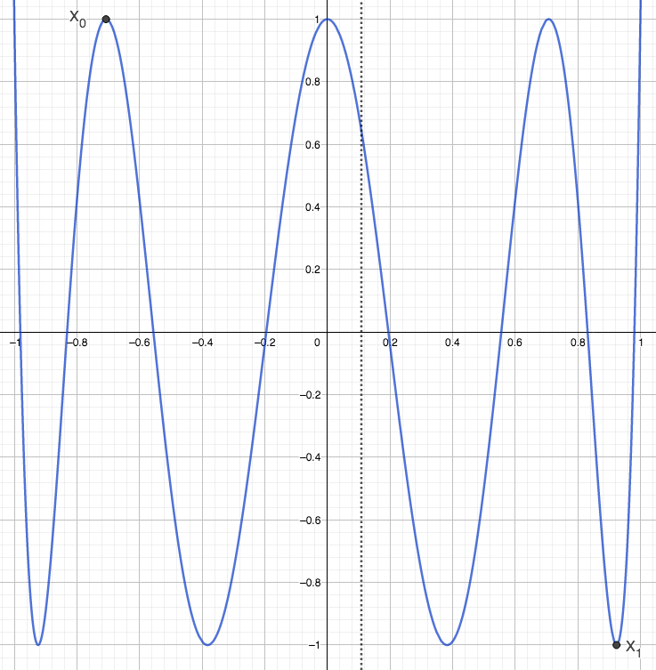
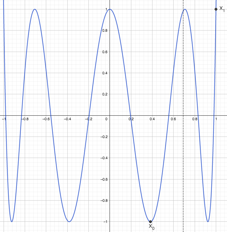
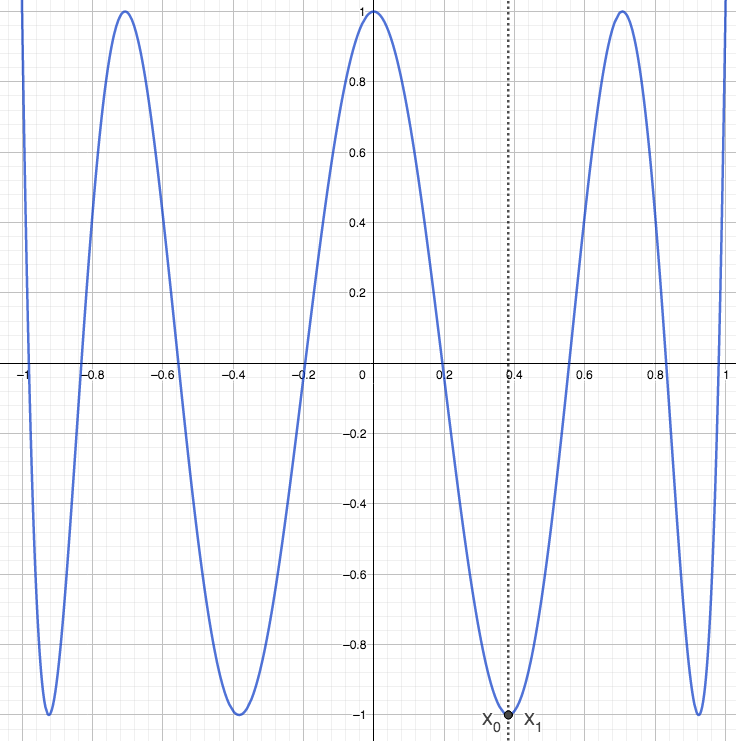
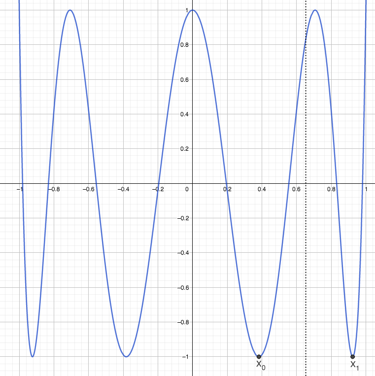
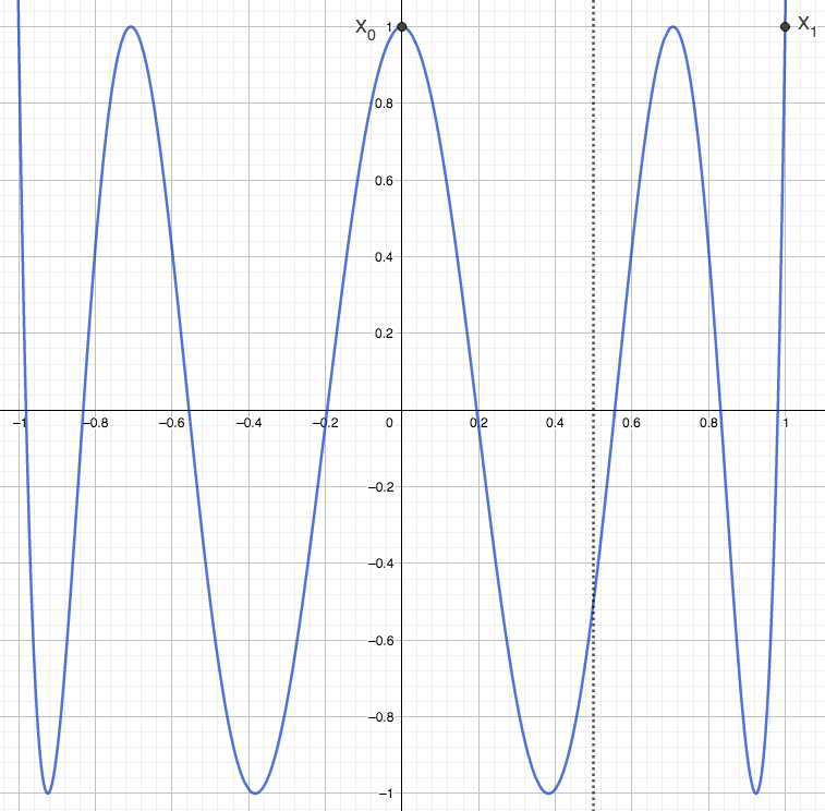
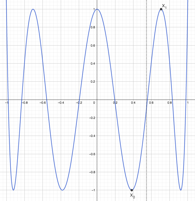
Figure 1. $\kappa=8$. $T_{\kappa=8}(x)$. Illustration of solutions $\mathcal{E}_{0}$ in system (6.1). Left to right : $\mathcal{E}_{0}=\cos(6\pi/\kappa)+\cos(\pi/\kappa)$, $\mathcal{E}_{0}=\cos(3\pi/\kappa)+1$, $\mathcal{E}_{0}=\cos(3\pi/\kappa)+\cos(3\pi/\kappa)$, $\mathcal{E}_{0}=\cos(3\pi/\kappa)+\cos(\pi/\kappa)$, $\mathcal{E}_{0}=\cos(4\pi/\kappa)+1$, $\mathcal{E}_{0}=\cos(2\pi/\kappa)+\cos(3\pi/\kappa)$.

7. A decreasing sequence of thresholds in $J_{2}(\kappa):=(2\cos(\pi/\kappa),1+\cos(\pi/\kappa))$

This entire section is in dimension 2. Using ideas of section 5 we prove the existence of a sequence of threshold energies $\in J_{2}:=(2\cos(\pi/\kappa),1+\cos(\pi/\kappa))$. Theorem 1.7 is a consequence of Propositions 7.1, 7.2, 7.3, 7.4. We state these Propositions now, and prove them at the end of the section. We also prove Proposition 1.8 and give justification for Conjecture 1.9.

Proposition 7.1.

(odd terms) Fix $\kappa\geq 2$, and let $n\in\mathbb{N}^{*}$ odd be given. System (5.1) admits a unique solution satisfying $\mathcal{E}_{n}\in J_{2}(\kappa)$ and

(7.1) $$\mathcal{E}_{n}-1=X_{0}<X_{1}<X_{2}<...<X_{(n-1)/2}$$

$$\quad\quad\quad\quad\quad\quad\quad\quad\quad\quad\quad\quad<\cos(\pi/\kappa)<X_{(n+1)/2}<...<X_{n}<X_{n+1}:=1.$$

Furthermore, this solution satisfies (5.2), (5.3) and (5.4), and so $\mathcal{E}_{n}\in\mathfrak{T}_{n,\kappa}$.

Proposition 7.2.

(even terms) Let $\kappa\geq 2$, and $n\in\mathbb{N}^{*}$ even be given. System (5.6) admits a unique solution satisfying $\mathcal{E}_{n}\in J_{2}(\kappa)$ and

(7.2) $$\mathcal{E}_{n}-1=X_{0}<X_{1}<X_{2}<...<X_{n/2}=\cos(\pi/\kappa)<X_{n/2+1}<...<X_{n}<X_{n+1}:=1.$$

Furthermore, this solution satisfies (5.7), (5.8) and (5.9), and so $\mathcal{E}_{n}\in\mathfrak{T}_{n,\kappa}$.

Figure 2 illustrates the solutions in Propositions 7.1 and 7.2 for $1\leq n\leq 6$ and $\kappa=3$. A few exact solutions are given in Table 1.

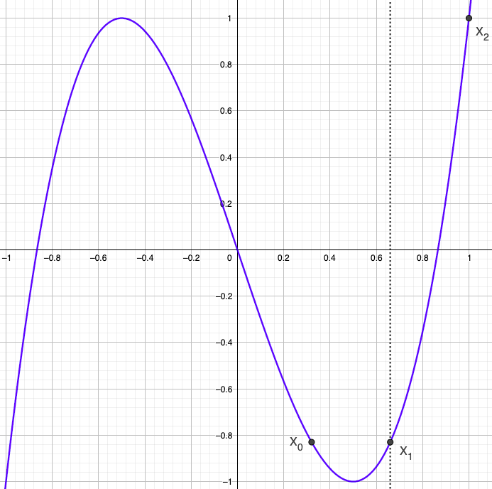
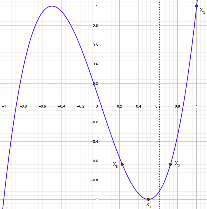
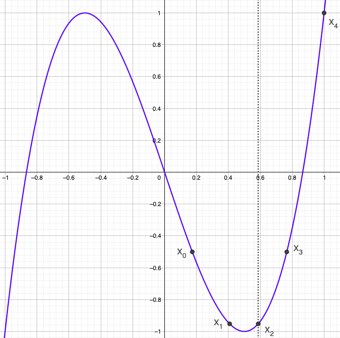
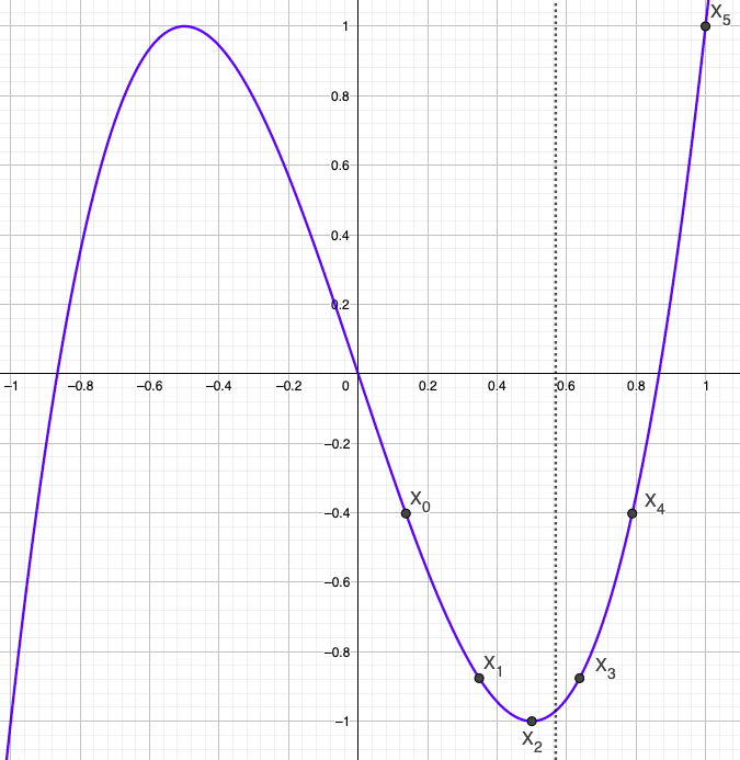
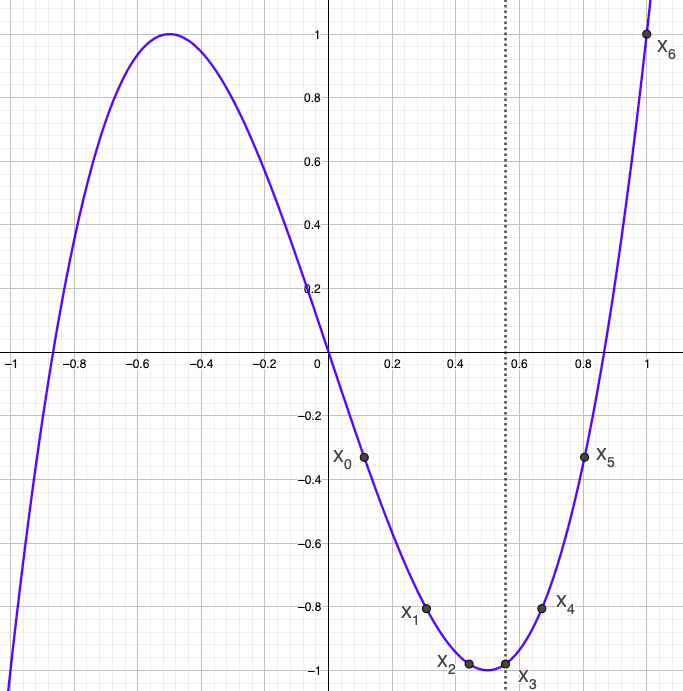
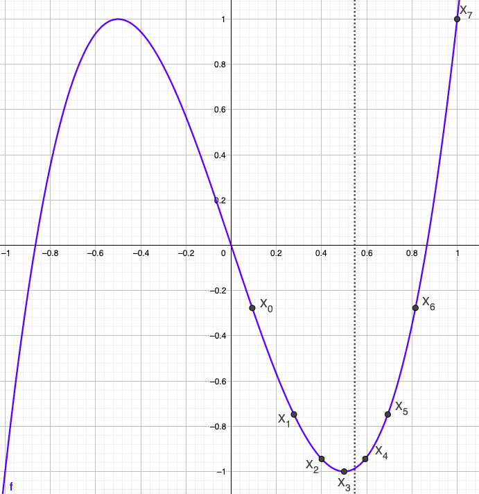
Figure 2. $T_{\kappa=3}(x)$. Solutions $\mathcal{E}_{n}$ in Propositions 7.1 and 7.2. Left to right : $\mathcal{E}_{1}\simeq 1.3207$, $\mathcal{E}_{2}\simeq 1.2287$, $\mathcal{E}_{3}\simeq 1.1737$, $\mathcal{E}_{4}\simeq 1.1375$, $\mathcal{E}_{5}\simeq 1.1121$, $\mathcal{E}_{6}\simeq 1.0934$.

Proposition 7.3.

Fix $\kappa\geq 2$. The odd and even energy solutions $\mathcal{E}_{n}$ of Propositions 7.1 and 7.2 interlace and are a strictly decreasing sequence : $\mathcal{E}_{n+2}<\mathcal{E}_{n+1}<\mathcal{E}_{n}$, $\forall n\in\mathbb{N}^{*}$.

Proposition 7.4.

Let $\mathcal{E}_{n}$ be the solutions in Propositions 7.1 and 7.2. Then $\mathcal{E}_{n}\searrow 2\cos(\pi/\kappa)$.

We now prove Proposition 1.8.

Proof of Proposition 1.8. Fix $\kappa=2$. We prove that the unique solutions of Prop. 7.1 and 7.2 are

$$\mathcal{E}_{n}=2/(2+n),\quad X_{q}=\mathcal{E}_{n}-1+q\mathcal{E}_{n},\quad q=0,...,n,\quad n\in\mathbb{N}^{*}.$$

In particular, $\mathcal{E}_{n}\searrow 0=\inf J_{2}$ and Conjecture 1.9 holds.

$\bullet$ Fix $n$ odd. $T_{2}(X_{q})=T_{2}(X_{n-q})\Leftrightarrow X_{q}=\pm X_{n-q}=\pm(\mathcal{E}_{n}-X_{q+1})$, $q=0,1,...,(n-1)/2$. Thanks to ordering (LABEL:chain_1) and $X_{(n+1)/2}=\mathcal{E}_{n}/2$ the appropriate sign is always $-$. Thus, recursively :

$$X_{0}=\mathcal{E}_{n}-1=-\mathcal{E}_{n}+\left(-\mathcal{E}_{n}+\left(...\right)\right)=-(n+1)\mathcal{E}_{n}/2+\mathcal{E}_{n}/2\Longrightarrow\mathcal{E}_{n}=2/(n+2).$$

$\bullet$ Fix $n$ even. We also have $X_{q}=\pm(\mathcal{E}_{n}-X_{q+1})$, $q=0,1,...,n/2-1$. Thanks to the ordering (7.2) and the fact that $X_{n/2}=0$ and we assume $\mathcal{E}_{n}\geq 0$ the appropriate sign is always $-$. Thus :

$$X_{0}=\mathcal{E}_{n}-1=-\mathcal{E}_{n}+\left(-\mathcal{E}_{n}+\left(...\right)\right)=-n\mathcal{E}_{n}/2\Longrightarrow\mathcal{E}_{n}=2/(n+2).$$

Moreover, finite induction shows that the system also implies $X_{q}=\mathcal{E}_{n}-1+q\mathcal{E}_{n}$, $q=1,2,...,n$. ∎

Remark 7.1.

As a consequence of the proof of Proposition 1.8, the distance between adjacent $X_{q}$’s is the same for $\kappa=2$ : $|X_{q}-X_{q+1}|\equiv\mathcal{E}_{n}$, $0\leq q\leq n$. This property is specific to $\kappa=2$.

Let us express the solutions $\mathcal{E}_{n}$ as solutions to a single equation for $\kappa=3,4$. To do this we need to select the appropriate branches of $T_{3}^{-1}$ and $T_{4}^{-1}$. Let

$$\begin{cases}f_{E}:x\mapsto\frac{-(E-x)+\sqrt{3}\sqrt{1-(E-x)^{2}}}{2}&\text{if}\ \kappa=3,\\ f_{E}:x\mapsto\sqrt{1-(E-x)^{2}}&\text{if}\ \kappa=4.\end{cases}$$

Figure 3 illustrates solutions $\mathcal{E}_{2n}(\kappa)$ of Proposition 7.5 for $\kappa=3,4$. In these graphs the slope of the orange trend line is close to $-2$, and this is our rationale behind Conjecture 1.9. Numerically we found similar behavior for $\kappa=5,6,8$, see [GM4]. Based on these graphs the interested reader could conjecture on the constant $c(\kappa)$ in Conjecture 1.9.

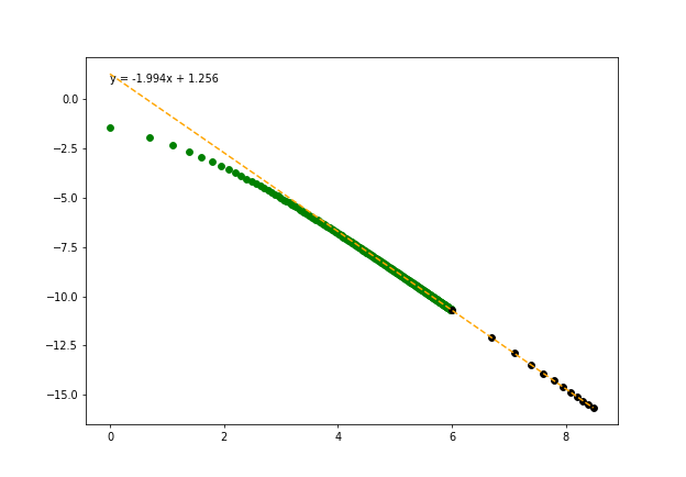
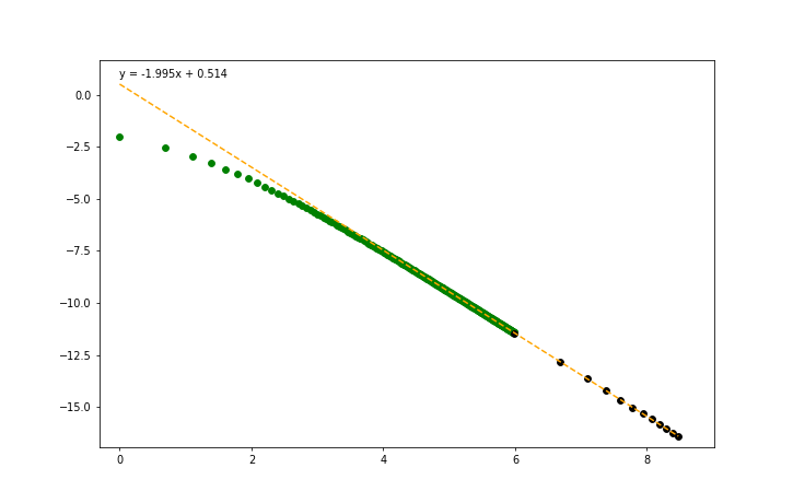
Figure 3. Graphs with $\log(n)$ on $x$-axis and $\log(\mathcal{E}_{2n}(\kappa)-2\cos(\pi/\kappa))$ on $y$-axis. Left : $\kappa=3$ ; Right : $\kappa=4$. Green dots are $1\leq n\leq 400$ ; black dots are $n=400,800,1200,...,4800$. Orange line is trend line based on linear regression of black dots.

Proposition 7.5.

Let $\kappa\in\{3,4\}$. Even terms: the $\mathcal{E}_{2n}$ in Theorem 1.7 are solution to the equation $\mathcal{E}_{2n}=1+f_{\mathcal{E}_{2n}}^{(n)}\left(\cos(\pi/\kappa)\right)$, $n\in\mathbb{N}^{*}$ ($f_{\mathcal{E}_{2n}}$ composed with itself $n$ times evaluated at $\cos(\pi/\kappa)$). Odd terms: the $\mathcal{E}_{2n-1}$ in Theorem 1.7 are solution to the equation $\mathcal{E}_{2n-1}=1+f_{\mathcal{E}_{2n-1}}^{(n)}(\frac{\mathcal{E}_{2n-1}}{2})$.

We now sequentially give the missing proofs of the aforementioned results in this section. We begin by a remark :

Remark 7.2.

Thanks to Lemma 2.5,

1. Given $\cos(2\pi/\kappa)<a<b<\cos(\pi/\kappa)$, there exist unique $\cos(\pi/\kappa)<b^{\prime}<a^{\prime}<1$ such that $T_{\kappa}(a)=T_{\kappa}(a^{\prime})>T_{\kappa}(b^{\prime})=T_{\kappa}(b)$.

2. Given $\cos(\pi/\kappa)<b^{\prime}<a^{\prime}<1$, there exist unique $\cos(2\pi/\kappa)<a<b<\cos(\pi/\kappa)$, such that $T_{\kappa}(a^{\prime})=T_{\kappa}(a)>T_{\kappa}(b)=T_{\kappa}(b^{\prime})$.

Moreover, $(a,b)$ depends bi-continuously on $(a^{\prime},b^{\prime})$.

Proof of Proposition 7.1.

We implement the dynamical algorithm for $n$ odd of section 5. Initialize energy $E$ to $E=E(\alpha)=2\cos(\pi/\kappa)+\alpha$ with $\alpha\in\mathbf{A}_{max}:=(0,1-\cos(\pi/\kappa))$. First, by Remark 5.2 we know $X_{(n+1)/2}=E/2=\cos(\pi/\kappa)+\alpha/2\in(\cos(\pi/\kappa),1)$. In particular when $\alpha\searrow 0_{+}$, note that $X_{(n+1)/2}\searrow\cos(\pi/\kappa)_{+}$. Now, up to a smaller $\alpha$ still within $\mathbf{A}_{max}$, we construct inductively and continuously in $\alpha$ all of the remaining $X_{q}=X_{q}(\alpha)$, by checking all the constraints of (5.1), (5.2) – (5.4), but with the exception of (5.3), i.e. $X_{n+1}=1\Leftrightarrow X_{0}=E-1$.

$\bullet$ $X_{(n-1)/2}$ is determined in $(\cos(2\pi/\kappa),\cos(\pi/\kappa))$ so that $T_{\kappa}(X_{(n-1)/2})=T_{\kappa}(X_{(n+1)/2})$. In particular, $X_{(n-1)/2}<\cos(\pi/\kappa)<X_{(n+1)/2}$. Note that $X_{(n-1)/2}\nearrow\cos(\pi/\kappa)_{-}$, as $\alpha\searrow 0_{+}$.

$\bullet$ $X_{(n+3)/2}$ is the symmetric of $X_{(n-1)/2}$ wrt. $X_{(n+1)/2}=E/2$. So $X_{(n+1)/2}<X_{(n+3)/2}$. Up to a smaller $\alpha$ possibly, $X_{(n+3)/2}\in(\cos(\pi/\kappa),1)$. As $\alpha\searrow 0_{+}$, $X_{(n+3)/2}\searrow\cos(\pi/\kappa)_{+}$.

$\bullet$ As per Remark 7.2, $\exists!X_{(n-3)/2}\in(\cos(2\pi/\kappa),\cos(\pi/\kappa))$ such that $X_{(n-3)/2}<X_{(n-1)/2}$ and $T_{\kappa}(X_{(n-1)/2})=T_{\kappa}(X_{(n+1)/2})<T_{\kappa}(X_{(n+3)/2})$. Again, $X_{(n-3)/2}\nearrow\cos(\pi/\kappa)_{-}$, as $\alpha\searrow 0_{+}$.

$\bullet$ $X_{(n+5)/2}$ is the symmetric of $X_{(n-3)/2}$ wrt. $X_{(n+1)/2}=E/2$. Up to a smaller $\alpha$ possibly, $X_{(n+5)/2}\in(\cos(\pi/\kappa),1)$. Since $X_{(n-3)/2}<X_{(n-1)/2}$, we infer $X_{(n+3)/2}<X_{(n+5)/2}$. In particular, $T_{\kappa}(X_{(n-3)/2})=T_{\kappa}(X_{(n+3)/2})<T_{\kappa}(X_{(n+5)/2})$. Once more, $X_{(n+5)/2}\searrow\cos(\pi/\kappa)_{+}$, as $\alpha\searrow 0_{+}$.

$\bullet$ We continue this ping pong game inductively till all of the $X_{q}=X_{q}(\alpha)$, $q=0,...,n+1$, have been defined. Note that the last step of the ping pong game was to place $X_{n+1}$ in such a way that it is the symmetric of $X_{0}$ wrt.  $X_{(n+1)/2}=E/2$ (2nd line of (5.1)). Now we consider the set $\mathbf{A}_{n}$ ($\mathbf{A}$ depends on $n$) of all the positive $\alpha$’s that allow a construction verifying :

(7.3) $$E-1\leq X_{0}<X_{1}<X_{2}<...<X_{(n-1)/2}<\cos(\pi/\kappa)<X_{(n+1)/2}<...<X_{n}<X_{n+1}\leq 1.$$

$\mathbf{A}_{n}\subset\mathbf{A}_{max}$ since if $\alpha\geq 1-\cos(\pi/\kappa)$, $X_{n+1}=E-X_{0}\geq 1+\cos(\pi/\kappa)-X_{0}\geq 1$. This observation will imply that $\mathcal{E}_{n}\in J_{2}(\kappa)$ when the proof is over. As a side note, it is not hard to see that $\mathbf{A}_{n+2}\subset\mathbf{A}_{n}$ ; later in this section we prove $\cap_{n\in\mathbb{N},\ n\ \text{odd}}\mathbf{A}_{n}=\emptyset$. It remains to argue that there is a unique $\alpha^{*}\in\mathbf{A}_{n}$ such that $X_{n+1}(\alpha^{*})=1\Leftrightarrow X_{0}(\alpha^{*})=E(\alpha^{*})-1$. First, note that by construction, the chain of strict inequalities in (7.3) remains valid as $\alpha$ increases in $\mathbf{A}_{n}$. Second, recall that $X_{n+1}\geq 1$ as $\alpha\geq 1-\cos(\pi/\kappa)$. Moreover, $X_{n+1}$ is strictly increasing for $\alpha\in\mathbf{A}_{n}$. Thirdly, and finally, note that by construction, as $\alpha$ increases in $\mathbf{A}_{n}$, $X_{n+1}$ must reach $1$ before $X_{0}$ reaches $\cos(2\pi/\kappa)$. This is because $T_{\kappa}(X_{0})=T_{\kappa}(X_{n})<T_{\kappa}(X_{n+1})$. Another way to see this is to argue by contradiction. If $X_{0}$ were to reach $\cos(2\pi/\kappa)$ before $X_{n+1}$ reaches $1$, then

$$2\cos(\pi/\kappa)-\cos(2\pi/\kappa)\leq E-\cos(2\pi/\kappa)=E-X_{0}=X_{n+1}<1\Rightarrow 2\cos(\pi/\kappa)-\cos(2\pi/\kappa)<1,$$

which is a false statement. Thus, $\exists!\alpha^{*}$ s.t. $X_{n+1}(\alpha^{*})=1$. The energy solution $\mathcal{E}_{n}$ is $E(\alpha^{*})$. ∎

Proof of Proposition 7.2.

We implement the dynamical algorithm for $n$ even of section 5, and mimick the proof of Proposition 7.1. The main difference is that this time $X_{n/2}:=\cos(\pi/\kappa)$. It implies that the values $X_{0},X_{1}$, …, $X_{n/2-1}$ will belong to $(\cos(2\pi/\kappa),\cos(\pi/\kappa))$, whereas the values $X_{n/2+1},X_{n/2+2}$, …, $X_{n}$ will belong to $(\cos(\pi/\kappa),1)$. $X_{n+1}$ will be placed ultimately so that it equals 1.

Initialize energy $E$ to $E=E(\alpha)=2\cos(\pi/\kappa)+\alpha$ with $\alpha\in\mathbf{A}_{max}:=(0,1-\cos(\pi/\kappa))$. First, $E/2=\cos(\pi/\kappa)+\alpha/2\in(\cos(\pi/\kappa),1)$. Now, up to a smaller $\alpha$ still within $\mathbf{A}_{max}$, we construct inductively and continuously in $\alpha$ all of the remaining $X_{q}=X_{q}(\alpha)$, by checking all the constraints of (5.6), (5.7) – (5.9), but with the exception of the $X_{n+1}$ condition in (5.8), i.e. $X_{n+1}=1\Leftrightarrow X_{0}=E-1$.

$\bullet$ $X_{n/2+1}$ is the symmetric of $X_{n/2}$ wrt. $E/2$. So $X_{n/2}<E/2<X_{n/2+1}=\cos(\pi/\kappa)+\alpha$. As per Remark 7.2, $X_{n/2-1}$ is constructed in $(\cos(2\pi/\kappa),\cos(\pi/\kappa))$ so that $T_{\kappa}(X_{n/2-1})=T_{\kappa}(X_{n/2+1})$. We turn to $X_{n/2+2}$ which is is the symmetric of $X_{n/2-1}$ wrt. $E/2$. Up to a smaller $\alpha$ possibly, $X_{n/2+2}\in(\cos(\pi/\kappa),1)$. As per Remark 7.2, there is a unique $X_{n/2-2}\in(\cos(2\pi/\kappa),\cos(\pi/\kappa))$ such that $X_{n/2-2}<X_{n/2-1}$ and $T_{\kappa}(X_{n/2-2})=T_{\kappa}(X_{n/2+2})>T_{\kappa}(X_{n/2+1})$.

$\bullet$ We continue this ping pong game inductively till all of the $X_{q}=X_{q}(\alpha)$, $q=0,...,n+1$, have been defined. Note that the last step of the ping pong game was to place $X_{n+1}$ in such a way that it is the symmetric of $X_{0}$ wrt.  $E/2$ (2nd line of (5.6)). Now we consider the set $\mathbf{A}_{n}$ ($\mathbf{A}$ depends on $n$) of all the positive $\alpha$’s that allow a construction verifying :

(7.4) $$E-1\leq X_{0}<X_{1}<X_{2}<...<X_{n/2}=\cos(\pi/\kappa)<X_{n/2+1}<...<X_{n}<X_{n+1}\leq 1.$$

$\mathbf{A}_{n}\subset\mathbf{A}_{max}$ since if $\alpha\geq 1-\cos(\pi/\kappa)$, $X_{n+1}=E-X_{0}\geq 1+\cos(\pi/\kappa)-X_{0}\geq 1$. As a side note, it is not hard to see that $\mathbf{A}_{n+2}\subset\mathbf{A}_{n}$ ; later in this section we prove $\cap_{n\in\mathbb{N},\ n\ \text{even}}\mathbf{A}_{n}=\emptyset$. It remains to argue that there is a unique $\alpha^{*}\in\mathbf{A}_{n}$ such that $X_{n+1}(\alpha^{*})=1\Leftrightarrow X_{0}(\alpha^{*})=E(\alpha^{*})-1$. First, note that by construction, the chain of strict inequalities in (7.4) remains valid as $\alpha$ increases in $\mathbf{A}_{n}$. Second, recall that $X_{n+1}\geq 1$ as $\alpha\geq 1-\cos(\pi/\kappa)$. Moreover, $X_{n+1}$ is strictly increasing for $\alpha\in\mathbf{A}_{n}$. Thirdly, and finally, note that by construction, as $\alpha$ increases in $\mathbf{A}_{n}$, $X_{n+1}$ must reach $1$ before $X_{0}$ reaches $\cos(2\pi/\kappa)$ (see the previous proof for the argument). Thus, $\exists!\alpha^{*}$ s.t. $X_{n+1}(\alpha^{*})=1$. The energy solution $\mathcal{E}_{n}$ is $E(\alpha^{*})$. ∎

Proof of Proposition 7.3.

Fix $n$ odd. So $n+1$ is even. Fix $E:=\min(\mathcal{E}_{n},\mathcal{E}_{n+1})$ (we suppose at this point that we don’t know which of the 2 energies is smaller) with $\mathcal{E}_{n}$ and $\mathcal{E}_{n+1}$ determined as in the proofs of Propositions 7.1 and 7.2 respectively. The construction gives $(X_{i,n}(E))_{i=0}^{n+1}$ satisfying (7.3) and $(X_{i,n+1}(E))_{i=0}^{n+2}$ satisfying (7.4). By the choice of $E$ we either have $X_{n+1,n}(E)=1$ or $X_{n+2,n+1}(E)=1$. This is to be determined. Starting from the bottom of the well we see that :

$$X_{(n-1)/2,n}(E)<X_{(n+1)/2,n+1}(E)=\cos(\pi/\kappa)<E/2=X_{(n+1)/2,n}(E)<X_{(n+1)/2+1,n+1}(E).$$

By the ping pong game that ensues, and using Remark 7.2, we inductively infer

$$X_{(n+1)/2+q,n}(E)<X_{(n+1)/2+q+1,n+1}(E),\quad\mbox{ for }q=0,1,...,(n+1)/2.$$

So $X_{n+1,n}(E)<X_{n+2,n+1}(E)$. It must be therefore that $X_{n+2,n+1}(E)=1$ and so $E=\mathcal{E}_{n+1}\leq\mathcal{E}_{n}$. Furthermore, $X_{n+1,n}(E)<X_{n+2,n+1}(E)$ implies $\mathcal{E}_{n+1}<\mathcal{E}_{n}$.

Fix $n$ even. So $n+1$ is odd. We proceed with the same setup as before. Fix $E:=\min(\mathcal{E}_{n},\mathcal{E}_{n+1})$ with $\mathcal{E}_{n}$ and $\mathcal{E}_{n+1}$ determined as in the proofs of Propositions 7.2 and 7.1 respectively. The construction gives $(X_{i,n}(E))_{i=0}^{n+1}$ satisfying (7.4) and $(X_{i,n+1}(E))_{i=0}^{n+2}$ satisfying (7.3). By the choice of $E$ we either have $X_{n+1,n}(E)=1$ or $X_{n+2,n+1}(E)=1$. This is to be determined. Starting from the bottom of the well we see that :

$$X_{n/2,n+1}(E)<X_{n/2,n}(E)=\cos(\pi/\kappa)<E/2=X_{n/2+1,n+1}(E)<X_{n/2+1,n}(E)$$

By the ping pong game that ensues, and using Remark 7.2, we inductively infer

$$X_{n/2+q,n}(E)<X_{n/2+q+1,n+1}(E),\quad\mbox{ for }q=0,1,...,n/2+1.$$

So $X_{n+1,n}(E)<X_{n+2,n+1}(E)$. It must be therefore that $X_{n+2,n+1}(E)=1$ and so $E=\mathcal{E}_{n+1}\leq\mathcal{E}_{n}$. Furthermore, $X_{n+1,n}(E)<X_{n+2,n+1}(E)$ implies $\mathcal{E}_{n+1}<\mathcal{E}_{n}$. ∎

Finally, to prove Proposition 7.4, we’ll start with a Lemma which characterizes a geometric property of the graph of $T_{\kappa}$ :

Lemma 7.6.

Let $\kappa\geq 2$. If $\cos(2\pi/\kappa)<a<\cos(\pi/\kappa)<b<1$ are such that $T_{\kappa}(a)=T_{\kappa}(b)$, then

(7.5) $$\cos(\pi/\kappa)-a>b-\cos(\pi/\kappa).$$

Proof. To prove this Lemma we analyze the function $S_{\kappa}(x):=T_{\kappa}(x)-T_{\kappa}(2\cos(\pi/\kappa)-x)$. If we can prove that $S_{\kappa}(x)>0$ on $(\cos(\pi/\kappa),1)$, then $T_{\kappa}(a)=T_{\kappa}(b)>T_{\kappa}(2\cos(\pi/\kappa)-b)$ for $b\in(\cos(\pi/\kappa),1)$ and $a\in(\cos(2\pi/\kappa),\cos(\pi/\kappa))$. This implies $a<2\cos(\pi/\kappa)-b$, i.e. (7.5) holds. Clearly $S_{\kappa}(\cos(\pi/\kappa))=0$. Thus, to prove that $S_{\kappa}(x)>0$ on $(\cos(\pi/\kappa),1)$ it is enough to prove that $S_{\kappa}$ is strictly increasing on $(\cos(\pi/\kappa),1)$. First note that

(7.6) $$\cos(2\pi/\kappa)<2\cos(\pi/\kappa)-x<\cos(\pi/\kappa),\quad\mbox{ for }x\in(\cos(\pi/\kappa),1).$$

We aim to show that $S_{\kappa}^{\prime}(x)>0$ for $x\in(\cos(\pi/\kappa),1)$. Fix $x\in(\cos(\pi/\kappa),1)$.

$$S_{\kappa}^{\prime}(x) =\kappa(U_{\kappa-1}(x)+U_{\kappa-1}(2\cos(\pi/\kappa)-x))$$

$$=\kappa 2^{\kappa-1}\left(\prod_{j=1}^{\kappa-1}(x-\cos(j\pi/\kappa))+\prod_{j=1}^{\kappa-1}(2\cos(\pi/\kappa)-x-\cos(j\pi/\kappa))\right)$$

$$=\kappa 2^{\kappa-1}(x-\cos(\pi/\kappa))\left(\prod_{j=2}^{\kappa-1}(x-\cos(j\pi/\kappa))-\prod_{j=2}^{\kappa-1}(2\cos(\pi/\kappa)-x-\cos(j\pi/\kappa))\right)$$

Since cosine is decreasing on $(0,\pi)$ and since (7.6) holds, note that $x-\cos(j\pi/\kappa)\geq x-\cos(\pi/\kappa)>0$ and $2\cos(\pi/\kappa)-x-\cos(j\pi/\kappa)>0$ for $j\in\{2,\ldots\kappa-1\}$. Next, for $j\in\{2,\ldots\kappa-1\}$, using again (7.6), note that

$$0<2\cos(\pi/\kappa)-x-\cos(j\pi/\kappa)<x-\cos(j\pi/\kappa).$$

Therefore, $S_{\kappa}^{\prime}$ is positive on $(\cos(\pi/\kappa),1)$. ∎

Remark 7.3.

$S_{\kappa}$ in Lemma 7.6 is stricly convex.

Proof of Proposition 7.4.

By Proposition 7.3 and since $\mathcal{E}_{n}>2\cos(\pi/\kappa)$, $\exists\ell$ such that $\mathcal{E}_{n}\searrow\ell\geq 2\cos(\pi/\kappa)$. It is enough to show that $\mathcal{E}_{2n+1}\to 2\cos(\pi/\kappa)$, $n\in\mathbb{N}^{*}$. Therefore, we suppose that $n$ is odd. We proceed by contradiction. Suppose $2\varepsilon:=\ell-2\cos(\pi/\kappa)>0$. Recall $X_{(n+1)/2,n}(\mathcal{E}_{n})=\mathcal{E}_{n}/2$. Then for all $n\geq 1$ and odd, $X_{(n+1)/2,n}(\mathcal{E}_{n})-\cos(\pi/\kappa)>\varepsilon$. Choose $n$ odd large enough so that $n\varepsilon>1$.

By Lemma 7.6, $\cos(\pi/\kappa)-X_{(n-1)/2,n}(\mathcal{E}_{n})>X_{(n+1)/2,n}(\mathcal{E}_{n})-\cos(\pi/\kappa)>\varepsilon$. Next, since $X_{(n-1)/2,n}(\mathcal{E}_{n})$ and $X_{(n+3)/2,n}(\mathcal{E}_{n})$ are symmetric wrt. the axis $x=\mathcal{E}_{n}/2$, it must be that $X_{(n+3)/2,n}(\mathcal{E}_{n})-\cos(\pi/\kappa)>3\varepsilon$. Again, apply Lemma 7.6 to get $\cos(\pi/\kappa)-X_{(n-3)/2,n}(\mathcal{E}_{n})>3\varepsilon$. Continuing in this way, we end up with $X_{(n+q)/2,n}(\mathcal{E}_{n})-\cos(\pi/\kappa)>q\varepsilon$ for $q=1,3,5,...,n$. But $X_{n,n}(\mathcal{E}_{n})>n\varepsilon>1$ is absurd. We conclude that $\ell=2\cos(\pi/\kappa)$. ∎

8. An increasing sequence of thresholds below $J_{3}(\kappa):=\left(1+\cos(2\pi/\kappa),2\cos(\pi/\kappa)\right)$

This entire section is in dimension 2. We prove the existence of a sequence of threshold energies $\mathcal{F}_{n}=\mathcal{F}_{n}(\kappa)\nearrow\inf J_{3}(\kappa)$. This section proves Theorem 1.13 for $\{\mathcal{F}_{n}\}$.

Proposition 8.1.

(odd terms) Fix $\kappa\geq 3$, and $n\in\mathbb{N}^{*}$ odd. System (5.1) has a unique solution (which we denote $\mathcal{F}_{n}$ instead of $\mathcal{E}_{n}$) such that $\mathcal{F}_{n}\in(\cos(\pi/\kappa)+\cos(2\pi/\kappa),1+\cos(2\pi/\kappa))$ and

(8.1) $$\cos(2\pi/\kappa)=:X_{n+1}<X_{n}<...<X_{(n+1)/2}=\mathcal{F}_{n}/2<X_{(n-1)/2}<...<X_{0}<1,$$

Furthermore, this solution satisfies (5.2), (5.3) and (5.4), and so $\mathcal{F}_{n}\in\mathfrak{T}_{n,\kappa}$.

Proposition 8.2.

(even terms) Fix $\kappa\geq 3$, and $n\in\mathbb{N}^{*}$ even. System (5.6) has a unique solution (which we denote $\mathcal{F}_{n}$ instead of $\mathcal{E}_{n}$) such that $\mathcal{F}_{n}\in(\cos(\pi/\kappa)+\cos(2\pi/\kappa),1+\cos(2\pi/\kappa))$ and

(8.2) $$\cos(2\pi/\kappa)=:X_{n+1}<X_{n}<...<X_{n/2}=\cos(\pi/\kappa)<X_{n/2-1}<...<X_{0}<1.$$

Furthermore, this solution satisfies (5.7), (5.8) and (5.9), and so $\mathcal{F}_{n}\in\mathfrak{T}_{n,\kappa}$.

Figure 4 illustrates the solutions in Propositions 8.1 and 8.2 for $1\leq n\leq 6$ and $\kappa=3$. Exact solutions for $\mathcal{F}_{1}$, $\mathcal{F}_{2}$ and $\mathcal{F}_{3}$ are :

$$\mathcal{F}_{1}=2/7,\quad\mathcal{F}_{2}=1/\sqrt{6},\quad\mathcal{F}_{3}=\frac{16}{247}+\frac{2\sqrt{2479}}{247}\cos\left(\frac{1}{3}\arctan\left(\frac{741\sqrt{2190}}{118457}\right)\right.$$

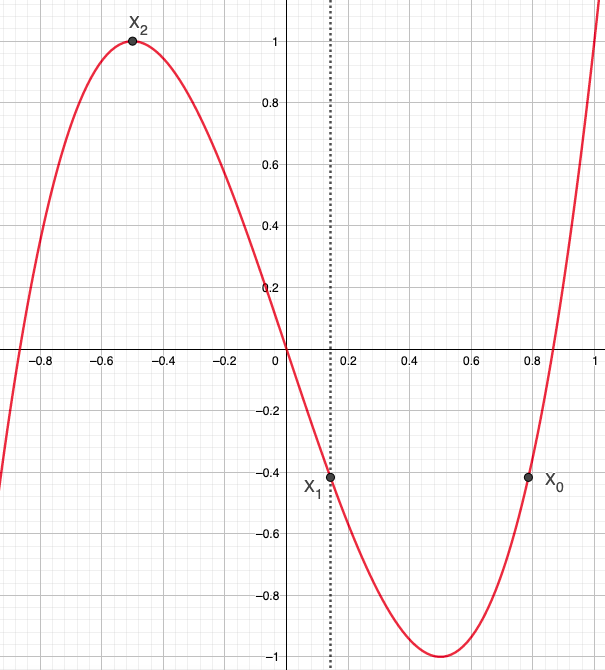
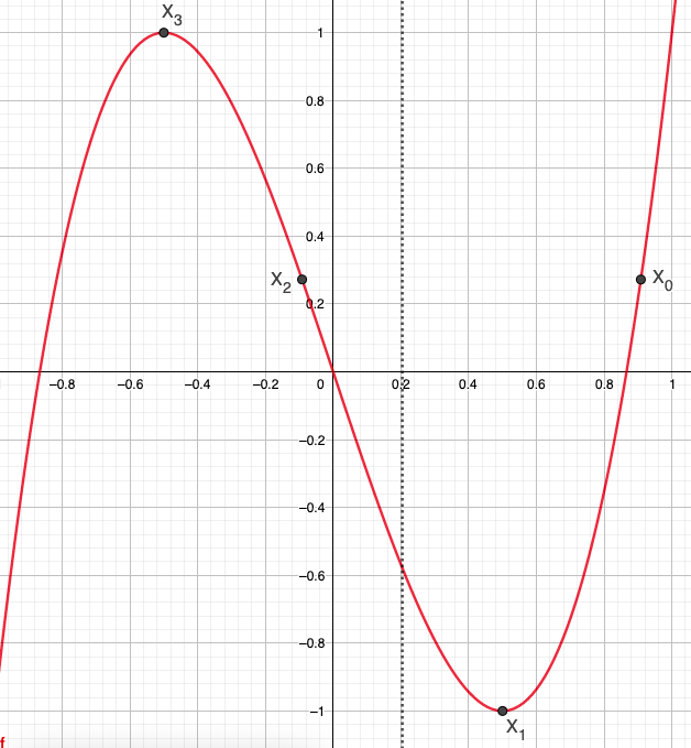
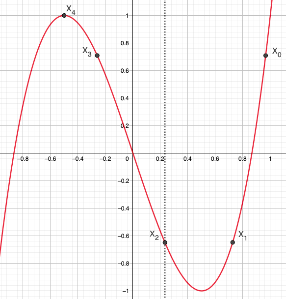
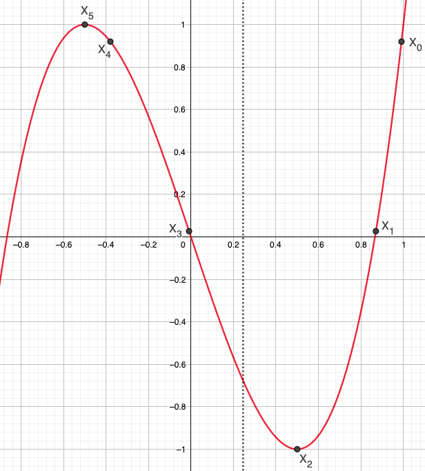
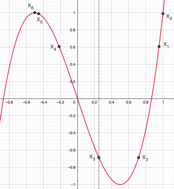
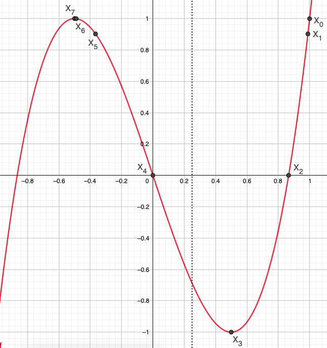
Figure 4. $\kappa=3$. $T_{\kappa=3}(x)$. $\mathcal{F}_{n}$ of Propositions 8.1 and 8.2. Left to right : $\mathcal{F}_{1}\simeq 0.2857$ ; $\mathcal{F}_{2}\simeq 0.40824$ ; $\mathcal{F}_{3}\simeq 0.46617$ ; $\mathcal{F}_{4}\simeq 0.49099$ ; $\mathcal{F}_{5}\simeq 0.49867$ ; $\mathcal{F}_{6}\simeq 0.499920$.

Proposition 8.3.

Fix $\kappa\geq 3$. The odd and even energy solutions $\mathcal{F}_{n}$ of Propositions 8.1 and 8.2 interlace and are a strictly increasing sequence : $\mathcal{F}_{n}<\mathcal{F}_{n+1}<\mathcal{F}_{n+2}$, $\forall n\in\mathbb{N}^{*}$. Also, $\mathcal{F}_{n}\nearrow\inf J_{3}:=1+\cos(2\pi/\kappa)$.

Remark 8.1.

Numerically we tried to compute several solutions $\mathcal{F}_{n}(\kappa=3)$ in order to conjecture the rate of convergence, but we struggled to get accurate numbers because of precision limitations. We found : $\mathcal{F}_{8}\simeq 0.4999999956$, which suggests $\mathcal{F}_{n}$ converges rather quickly to $\inf J_{3}$.

9. Another increasing sequence of thresholds below $J_{3}(\kappa)$

We revisit the sequence of the previous section but add a twist to it. The twist is that instead of placing $X_{0}$ on the branch of $T_{\kappa}$ to the right of $X_{n}$ we place it on the branch of $T_{\kappa}$ to the left of $X_{n}$; and instead of placing $X_{n+1}$ at $\cos(2\pi/\kappa)$, we place it at $1$. This gives a sequence which we believe is distinct. This section proves Theorem 1.13 for $\{\mathcal{G}_{n}\}$.

Proposition 9.1.

(odd terms) Fix $\kappa\geq 3$, and $n\in\mathbb{N}^{*}$ odd. System (5.1) has a unique solution (which we denote $\mathcal{G}_{n}$ instead of $\mathcal{E}_{n}$) such that $\mathcal{G}_{n}\in(\cos(\pi/\kappa)+\cos(2\pi/\kappa),1+\cos(2\pi/\kappa))$ and

(9.1) $$\mathcal{G}_{n}-1=X_{0}<X_{n}<X_{n-1}<...<X_{(n+1)/2}<X_{(n-1)/2}<...<X_{1}<X_{n+1}:=1.$$

Furthermore, this solution satisfies (5.2), (5.3) and (5.4), and so $\mathcal{G}_{n}\in\mathfrak{T}_{n,\kappa}$.

Remark 9.1.

The proof reveals that $X_{0}\in(\cos(3\pi/\kappa),\cos(2\pi/\kappa))$, $X_{n}$, $X_{n-1}$, …, $X_{(n+1)/2}\in(\cos(2\pi/\kappa),\cos(\pi/\kappa))$, and for $n\geq 3$, $X_{(n-1)/2}$,…, $X_{1}\in(\cos(\pi/\kappa),1)$. This is important because it means that $U_{\kappa-1}(X_{0})>0$, $U_{\kappa-1}(X_{n})$, …, $U_{\kappa-1}(X_{(n+1)/2})<0$, and for $n\geq 3$, $U_{\kappa-1}(X_{(n-1)/2})$, …, $U_{\kappa-1}(X_{1})>0$.

Proposition 9.2.

(even terms) Fix $\kappa\geq 3$, and $n\in\mathbb{N}^{*}$ even. System (5.6) has a unique solution (which we denote $\mathcal{G}_{n}$ instead of $\mathcal{E}_{n}$) such that $\mathcal{G}_{n}\in(\cos(\pi/\kappa)+\cos(2\pi/\kappa),1+\cos(2\pi/\kappa))$ and

(9.2) $$\mathcal{G}_{n}-1=X_{0}<X_{n}<X_{n-1}<...<X_{n/2+1}<X_{n/2}:=\cos(\pi/\kappa)<...<X_{1}<X_{n+1}:=1.$$

Furthermore, this solution satisfies (5.7), (5.8) and (5.9), and so $\mathcal{G}_{n}\in\mathfrak{T}_{n,\kappa}$.

Remark 9.2.

The proof reveals that $X_{0}\in(\cos(3\pi/\kappa),\cos(2\pi/\kappa))$, $X_{n}$, $X_{n-1}$, …, $X_{n/2+1}\in(\cos(2\pi/\kappa),\cos(\pi/\kappa))$, and for $n\geq 4$, $X_{n/2-1}$, …, $X_{1}\in(\cos(\pi/\kappa),1)$. This is important because it means that $U_{\kappa-1}(X_{0})>0$, $U_{\kappa-1}(X_{n})$, …, $U_{\kappa-1}(X_{n/2+1})<0$, and for $n\geq 4$, $U_{\kappa-1}(X_{n/2-1})$, …, $U_{\kappa-1}(X_{1})>0$.

Figure 5 illustrates the solutions in Propositions 9.1 and 9.2 for $1\leq n\leq 6$ and $\kappa=3$. Exact solutions for $\mathcal{G}_{1}$, $\mathcal{G}_{2}$ and $\mathcal{G}_{3}$ are :

$$\mathcal{G}_{1}=(5-3\sqrt{2})/7\simeq 0.10819,\quad\mathcal{G}_{2}=(9-\sqrt{33})/12\simeq 0.27129,$$

$$\mathcal{G}_{3}=\frac{1}{247}\left(\frac{199}{2}+\frac{1}{2}\sqrt{16838+a+b}-\frac{1}{2}\sqrt{32766-a-b+\frac{4340412}{\sqrt{16383+a+b}}}\right)\simeq 0.382291,$$

$$a:=\frac{1}{3}(39558654304767-2109209004864\sqrt{327})^{1/3},\quad b:=741(3601+192\sqrt{327})^{1/3}.$$

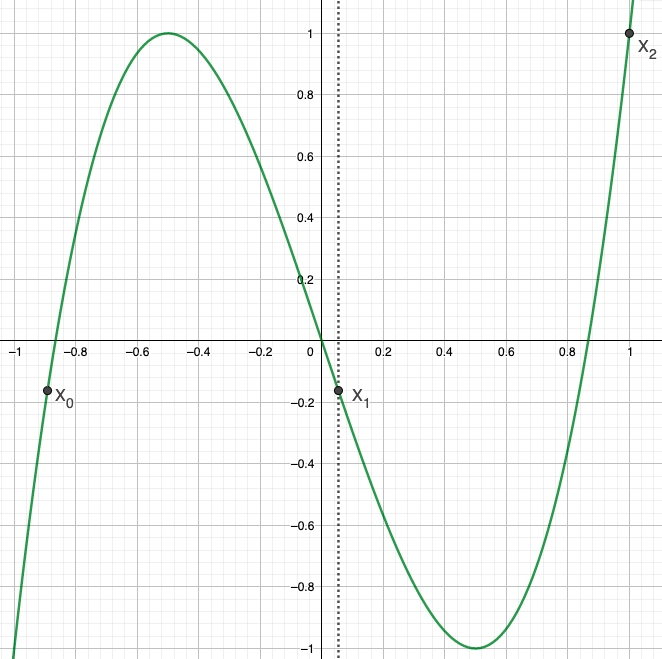
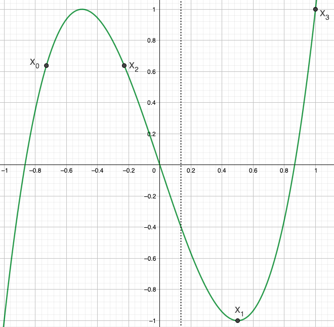
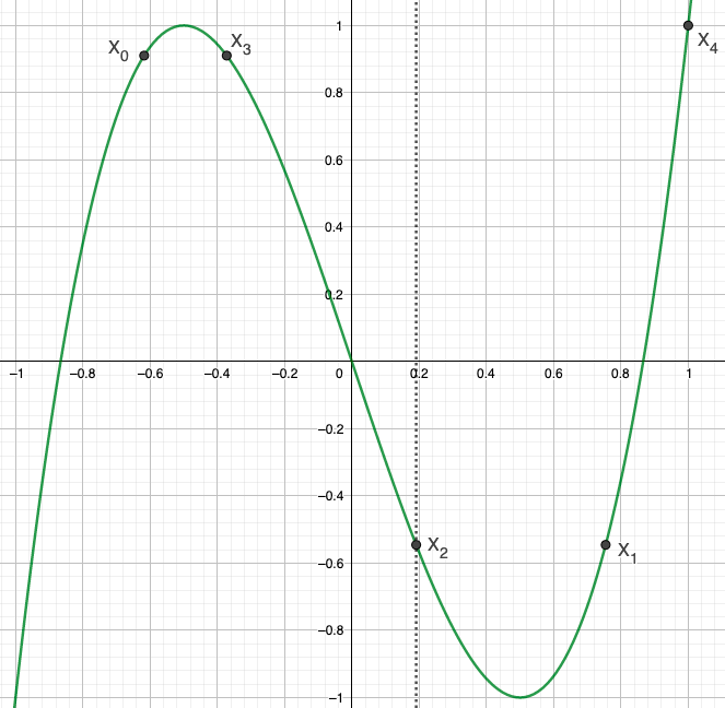
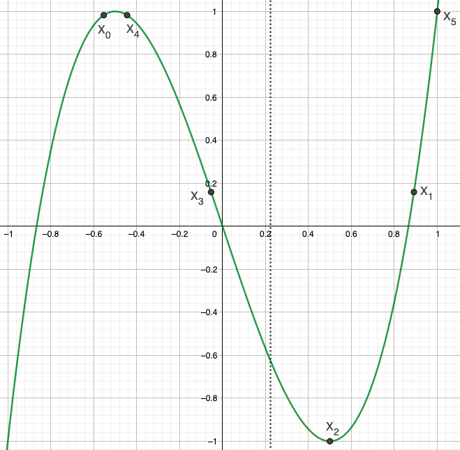
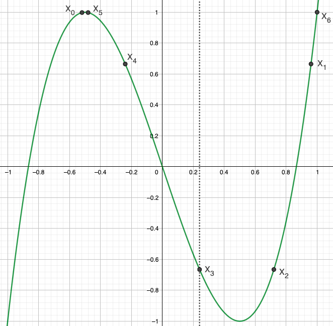
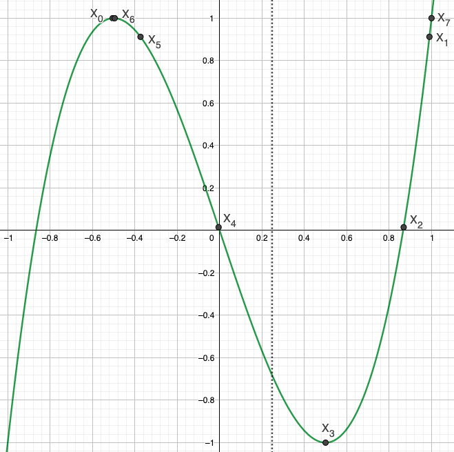
Figure 5. $\kappa=3$. $T_{\kappa=3}(x)$. $\mathcal{G}_{n}$ of Propositions 9.1 and 9.2. Left to right : $\mathcal{G}_{1}\simeq 0.10819$ ; $\mathcal{G}_{2}\simeq 0.27129$ ; $\mathcal{G}_{3}\simeq 0.382291$ ; $\mathcal{G}_{4}\simeq 0.446704$ ; $\mathcal{G}_{5}\simeq 0.480492$ ; $\mathcal{G}_{6}\simeq 0.495054$.

To justify $\mathcal{G}_{n}\in(\cos(\pi/\kappa)+\cos(2\pi/\kappa),1+\cos(2\pi/\kappa))$ for $n$ even, we know that we want $X_{n/2+1}\in(\cos(2\pi/\kappa),\cos(\pi/\kappa))$, and since $X_{n/2}=\cos(\pi/\kappa)$ and $X_{n/2+1}$ is the symmetric of $X_{n/2}$ wrt. $\mathcal{G}_{n}/2$, it must be that $\mathcal{G}_{n}-X_{n/2}=\mathcal{G}_{n}-\cos(\pi/\kappa)\in(\cos(2\pi/\kappa),\cos(\pi/\kappa))$, i.e. $\cos(2\pi/\kappa)+\cos(\pi/\kappa)\leq\mathcal{G}_{n}\leq 2\cos(\pi/\kappa)$. For the upper bound, we know that $X_{0}+X_{n+1}=X_{0}+1=\mathcal{G}_{n}$ and $X_{0}<\cos(2\pi/\kappa)$, so $\mathcal{G}_{n}<1+\cos(2\pi/\kappa)$. For $n$ odd we probably can get the range by using the interlacing property.

Proposition 9.3.

Fix $\kappa\geq 3$. The odd and even energy solutions $\mathcal{G}_{n}$ of Propositions 9.1 and 9.2 interlace and are a strictly increasing sequence : $\mathcal{G}_{n}<\mathcal{G}_{n+1}<\mathcal{G}_{n+2}$, $\forall n\in\mathbb{N}^{*}$. Also, $\mathcal{G}_{n}\nearrow\inf J_{3}:=1+\cos(2\pi/\kappa)$ as $n\to\infty$.

10. A generalization of section 7 : a sequence $\mathcal{E}_{n}\searrow 2\cos(j\pi/\kappa)$

The construction used to get a sequence in the right-most well of $T_{\kappa}(x)$ in section 7 is not specific to the right-most well. One can build a similar sequence in other wells.

10.1. Decreasing sequence in upright well, $j$ odd

Figure 6 illustrates a decreasing sequence $\mathcal{E}_{n}\searrow 2\cos(3\pi/\kappa)$, for $\kappa=8$, $j=3$. Note that the dotted line $x=\mathcal{E}_{n}/2$ is to the right of the minimum $x=\cos(3\pi/\kappa)$ but converges to it.

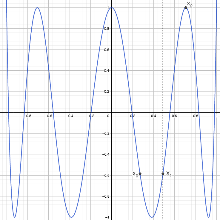
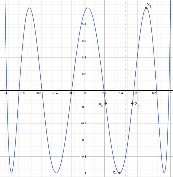
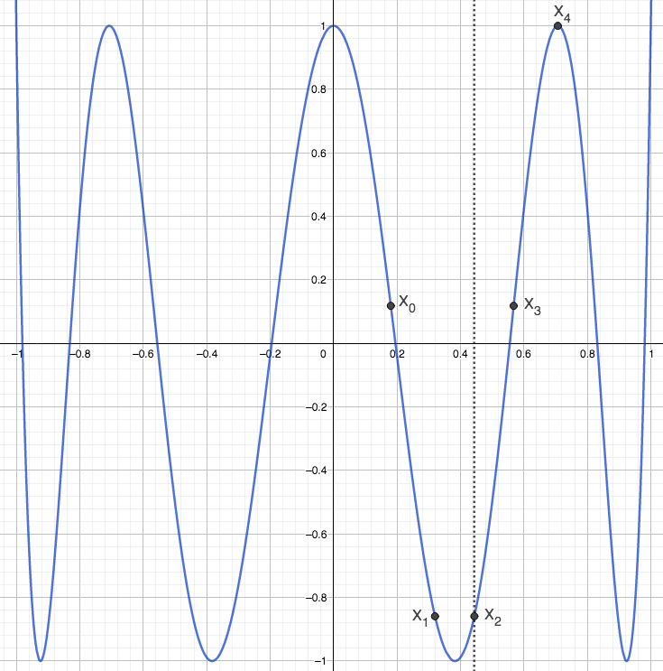
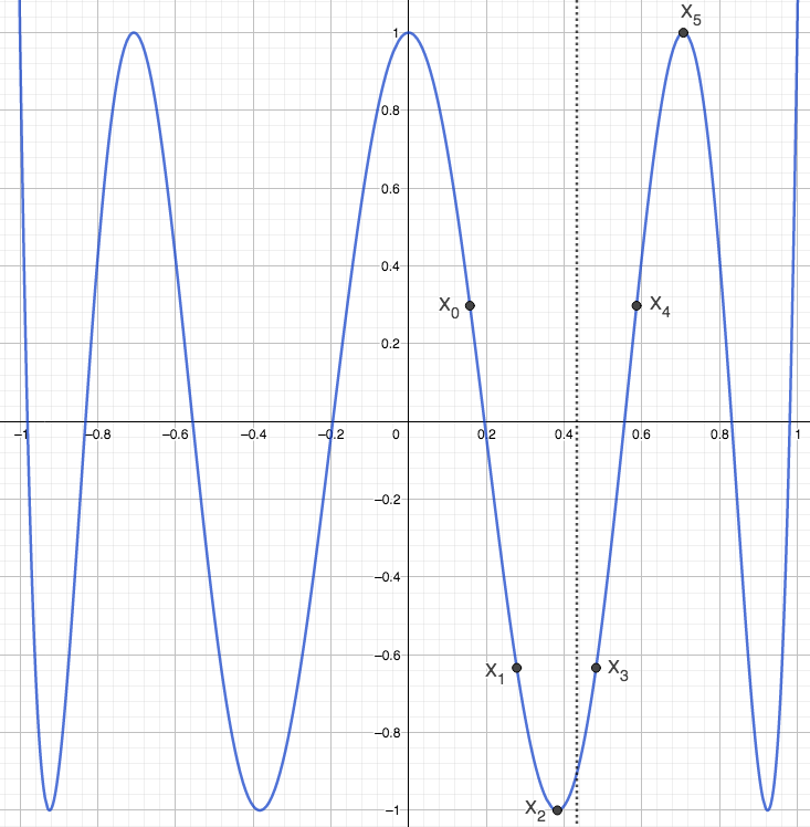
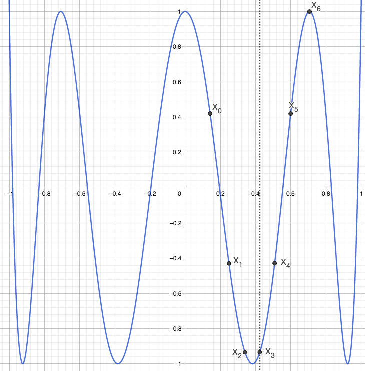
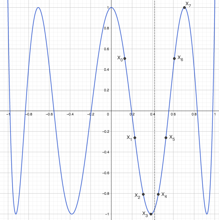
Figure 6. $T_{\kappa=8}(x)$. Solutions $\mathcal{E}_{n}$. Left to right : $\mathcal{E}_{1}\simeq 0.9781$, $\mathcal{E}_{2}\simeq 0.9216$, $\mathcal{E}_{3}\simeq 0.8877$, $\mathcal{E}_{4}\simeq 0.8650$, $\mathcal{E}_{5}\simeq 0.8488$, $\mathcal{E}_{6}\simeq 0.8368$.

Thus, we propose a generalization of Theorem 1.7 :

Theorem 10.1.

Fix $\kappa\geq 2$. Fix $1\leq j\leq\left\lfloor\kappa/2\right\rfloor$, $j$ odd. There is a sequence $\{\mathcal{E}_{n}\}_{n=1}^{\infty}$, which depends on $\kappa$, s.t. $\{\mathcal{E}_{n}\}\subset(2\cos(j\pi/\kappa),\cos((j-1)\pi/\kappa)+\cos((j+1)\pi/\kappa))\cap\bm{\Theta}_{\kappa}(\Delta)$, and $\mathcal{E}_{n+2}<\mathcal{E}_{n+1}<\mathcal{E}_{n}$, $\forall n\in\mathbb{N}^{*}$. Also, $\mathcal{E}_{2n-1}$, $\mathcal{E}_{2n}\in\bm{\Theta}_{n,\kappa}(\Delta)$, $\forall n\geq 1$, and

(10.1) $$\mathcal{E}_{n}-\cos((j-1)\pi/\kappa)=X_{0}<X_{1}<...<X_{n}<X_{n+1}:=\cos((j-1)\pi/\kappa).$$

10.2. Decreasing sequence in upside down well, $j$ even

For $j$ even, the well is upside down. Figure 7 illustrates a decreasing sequence $\mathcal{E}_{n}\searrow 2\cos(2\pi/\kappa)$, for $\kappa=8$, $j=2$. Note that the dotted line $x=\mathcal{E}_{n}/2$ is to the right of the maximum $x=\cos(2\pi/\kappa)$ but converges to it.

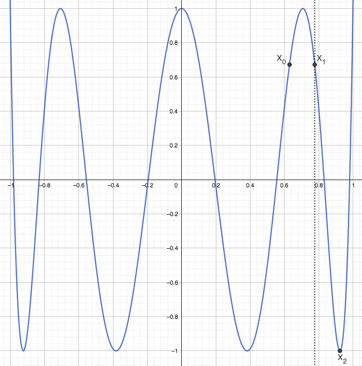
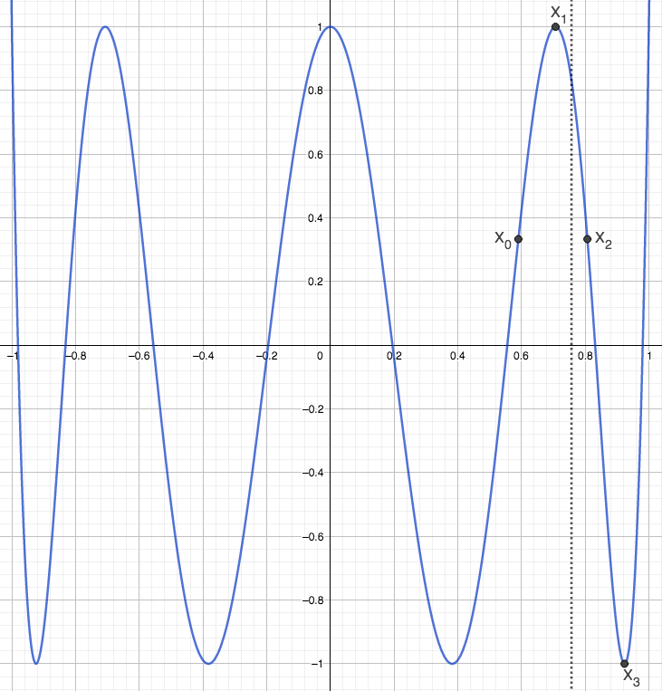
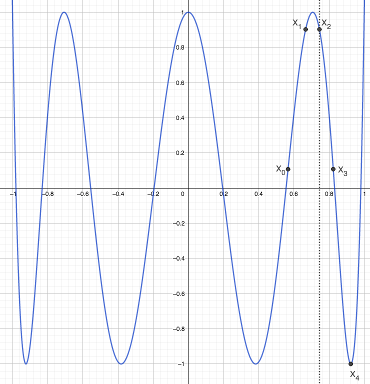
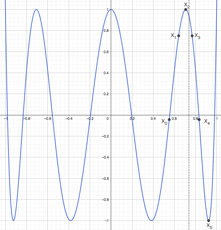
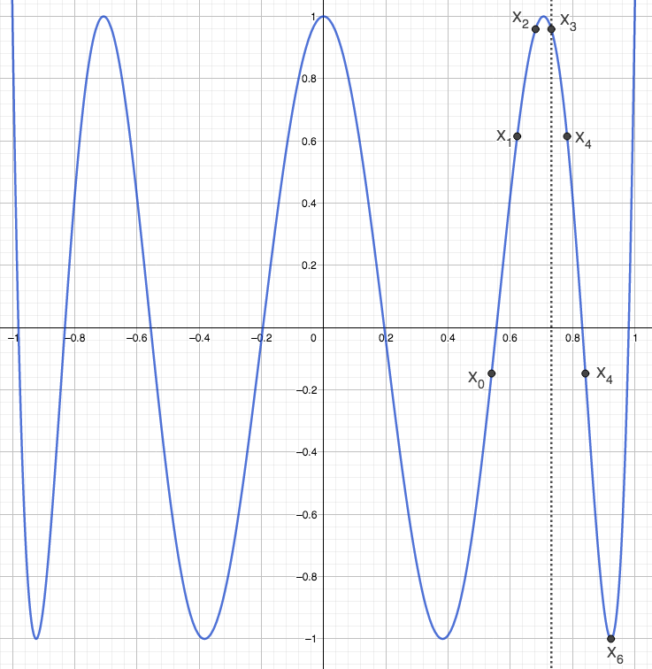
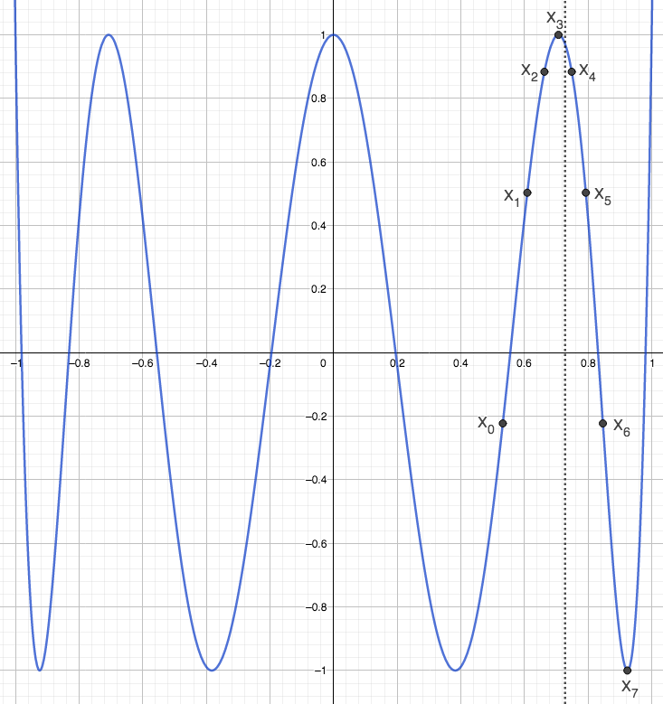
Figure 7. $T_{\kappa=8}(x)$. Solutions $\mathcal{E}_{n}$. Left to right : $\mathcal{E}_{1}\simeq 1.5536$, $\mathcal{E}_{2}\simeq 1.5142$, $\mathcal{E}_{3}\simeq 1.4906$, $\mathcal{E}_{4}\simeq 1.4750$, $\mathcal{E}_{5}\simeq 1.4640$, $\mathcal{E}_{6}\simeq 1.4559$.

Thus, we propose a generalization of Theorem 1.7 :

Theorem 10.2.

Fix $\kappa\geq 2$. Fix $2\leq j\leq\left\lfloor\kappa/2\right\rfloor$, $j$ even. There is a sequence $\{\mathcal{E}_{n}\}_{n=1}^{\infty}$, which depends on $\kappa$, s.t. $\{\mathcal{E}_{n}\}\subset(2\cos(j\pi/\kappa),\cos((j-1)\pi/\kappa)+\cos((j+1)\pi/\kappa))\cap\bm{\Theta}_{\kappa}(\Delta)$, and $\mathcal{E}_{n+2}<\mathcal{E}_{n+1}<\mathcal{E}_{n}$, $\forall n\in\mathbb{N}^{*}$. Also, $\mathcal{E}_{2n-1}$, $\mathcal{E}_{2n}\in\bm{\Theta}_{n,\kappa}(\Delta)$, $\forall n\geq 1$, and

(10.2) $$\mathcal{E}_{n}-\cos((j-1)\pi/\kappa)=X_{0}<X_{1}<...<X_{n}<X_{n+1}:=\cos((j-1)\pi/\kappa).$$

10.3. A comment on the proofs of these Theorems and a Conjecture on the limit

To prove the Theorems 10.1 and 10.2 one needs to adapt the proofs of Propositions 7.1, 7.2 and 7.3. The adaptation of these Propositions is straightforward. As for the limit we conjecture :

Conjecture 10.3.

Let $\{\mathcal{E}_{n}\}$ be the sequence in Theorems 10.1 and 10.2. Then $\mathcal{E}_{n}\searrow 2\cos(j\pi/\kappa)$.

To prove this conjecture we tried adapting the proofs of Proposition 7.4 and Lemma 7.6 but to no avail. To adapt the Lemma however, we do conjecture :

Conjecture 10.4.

Let $\kappa\geq 2$. Fix $1\leq j\leq\left\lfloor\kappa/2\right\rfloor$. If $\cos((j+1)\pi/\kappa)<a<\cos(j\pi/\kappa)<b<\cos((j-1)\pi/\kappa)$ are such that $T_{\kappa}(a)=T_{\kappa}(b)$, then

(10.3) $$\cos(j\pi/\kappa)-a>b-\cos(j\pi/\kappa).$$

We don’t know how to adapt the proof of Lemma 7.6 to prove Conjecture 10.4. We would want to prove that the function $S_{\kappa}(x):=T_{\kappa}(x)-T_{\kappa}(2\cos(j\pi/\kappa)-x)$ is positive for $x\in\left(\cos(j\pi/\kappa),\cos((j-1)\pi/\kappa)\right)$, for $j=1,2,..,\left\lfloor\kappa/2\right\rfloor$. We speculate this statement is true for $j=1,2,..,\left\lfloor\kappa/2\right\rfloor$. However the statement that $S_{\kappa}^{\prime}(x)\geq 0$ appears to be true only for $j=1$.

11. A generalization of section 8 : a sequence $\mathcal{F}_{n}\nearrow\cos((j-1)\pi/\kappa)+\cos((j+1)\pi/\kappa)$

Again, the construction used to get a sequence in the right-most well of $T_{\kappa}(x)$ in section 8 is not specific to the right-most well. One can build a similar sequence in other wells. In this section we get an increasing sequence $\mathcal{F}_{n}$. At first, it may be tempting to think that $\mathcal{F}_{n}\nearrow 2\cos(j\pi/\kappa)$, but this is not the case because $\cos((j-1)\pi/\kappa)+\cos((j+1)\pi/\kappa)<2\cos(j\pi/\kappa)$. Instead, we have $\mathcal{F}_{n}\nearrow\cos((j-1)\pi/\kappa)+\cos((j+1)\pi/\kappa)$.

11.1. Increasing sequence in upright well, $j$ odd

Figure 8 illustrates an increasing sequence $\mathcal{F}_{n}\nearrow\cos(4\pi/\kappa)+\cos(2\pi/\kappa)$, for $\kappa=8$, $j=3$. Note that the dotted line $x=\mathcal{F}_{n}/2$ is to the left of the minimum $x=\cos(3\pi/\kappa)$, approaches it, but converges before.

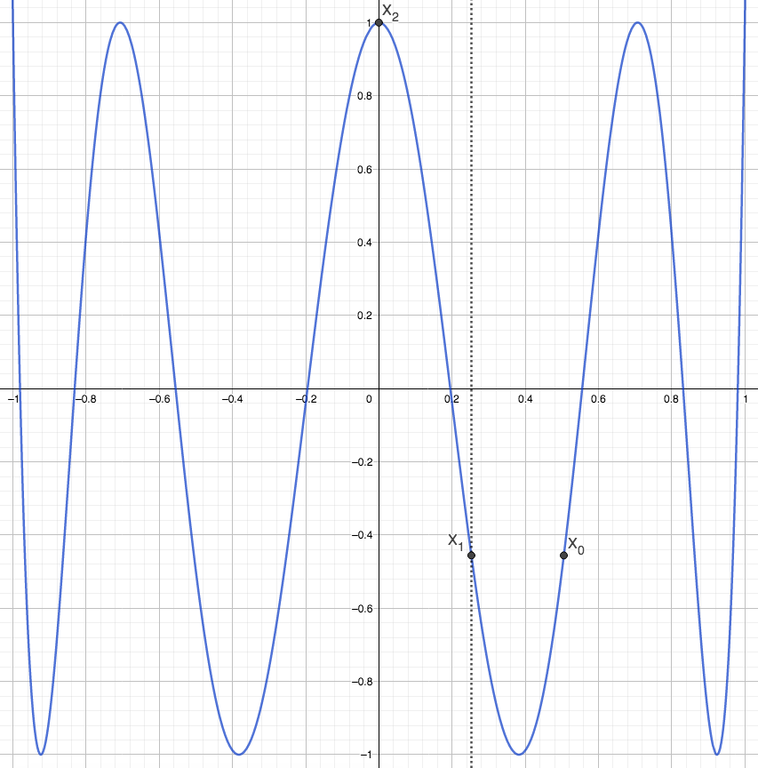
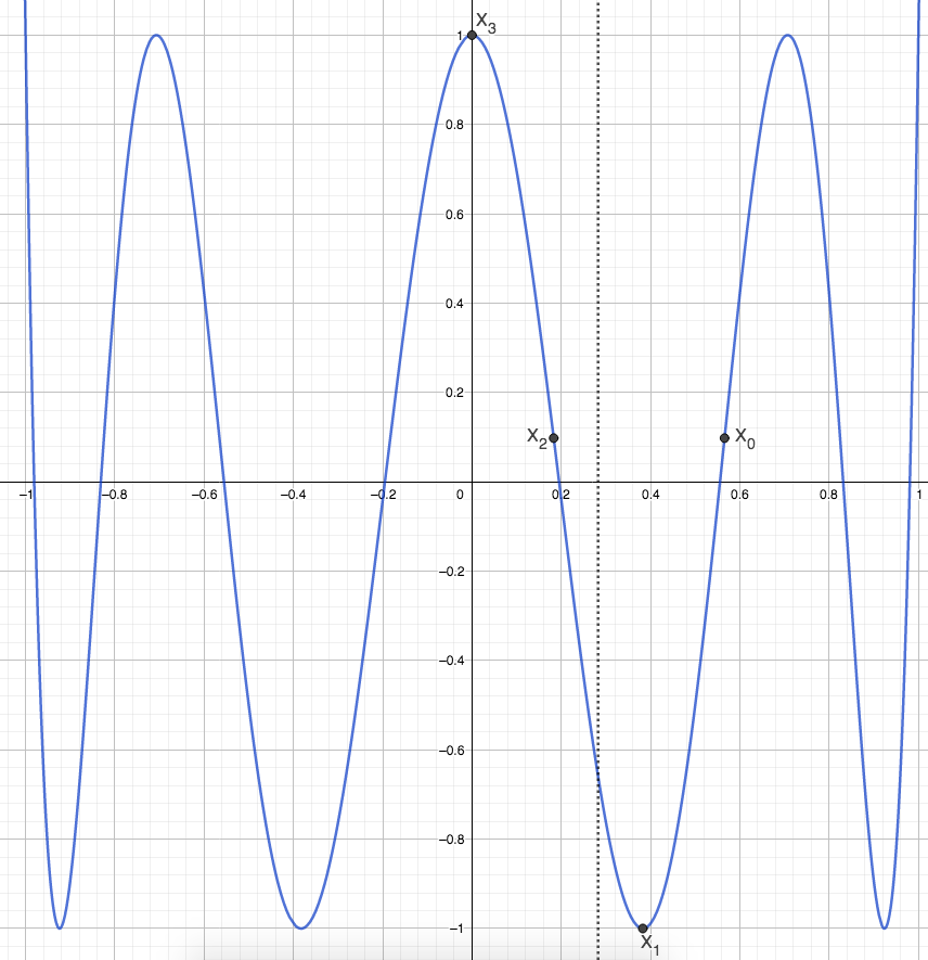
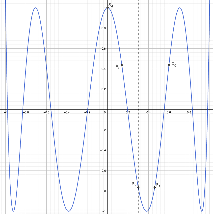
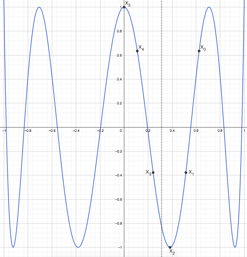
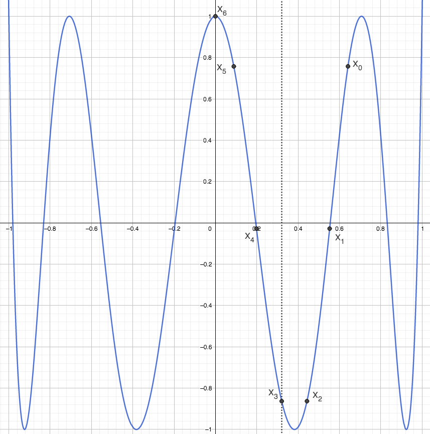
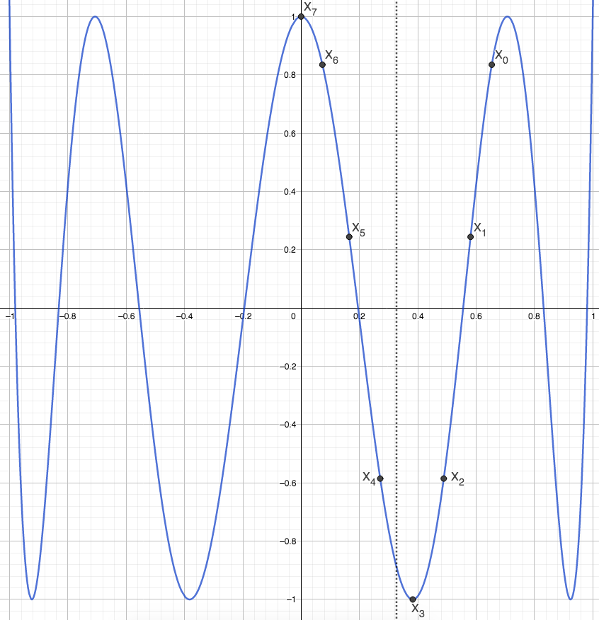
Figure 8. $T_{\kappa=8}(x)$. Solutions $\mathcal{F}_{n}$. Left to right : $\mathcal{F}_{1}\simeq 0.5054$, $\mathcal{F}_{2}\simeq 0.5657$, $\mathcal{F}_{3}\simeq 0.6014$, $\mathcal{F}_{4}\simeq 0.6249$, $\mathcal{F}_{5}\simeq 0.6415$, $\mathcal{F}_{6}\simeq 0.6537$.

Thus, we propose a generalization :

Theorem 11.1.

Fix $\kappa\geq 2$. Fix $1\leq j\leq\left\lfloor\kappa/2\right\rfloor$, $j$ odd. There is a sequence $\{\mathcal{F}_{n}\}_{n=1}^{\infty}$, which depends on $\kappa$, s.t. $\{\mathcal{F}_{n}\}\subset(2\cos((j+1)\pi/\kappa),\cos((j-1)\pi/\kappa)+\cos((j+1)\pi/\kappa))\cap\bm{\Theta}_{\kappa}(\Delta)$, and $\mathcal{F}_{n}<\mathcal{F}_{n+1}<\mathcal{F}_{n+2}$, $\forall n\in\mathbb{N}^{*}$. Also, $\mathcal{F}_{2n-1}$, $\mathcal{F}_{2n}\in\bm{\Theta}_{n,\kappa}(\Delta)$, $\forall n\geq 1$, and

(11.1) $$\cos((j+1)\pi/\kappa)=:X_{n+1}<X_{n}<...<X_{1}<X_{0}<\cos((j-1)\pi/\kappa).$$

11.2. Increasing sequence in upside down well, $j$ even

For $j$ even, the well is upside down. Figure 9 illustrates an increasing sequence $\mathcal{F}_{n}\nearrow\cos(3\pi/\kappa)+\cos(\pi/\kappa)$, for $\kappa=8$, $j=2$. Note that the dotted line $x=\mathcal{F}_{n}/2$ is to the left of the maximum $x=\cos(2\pi/\kappa)$, approaches it, but converges before.

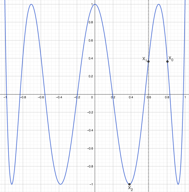
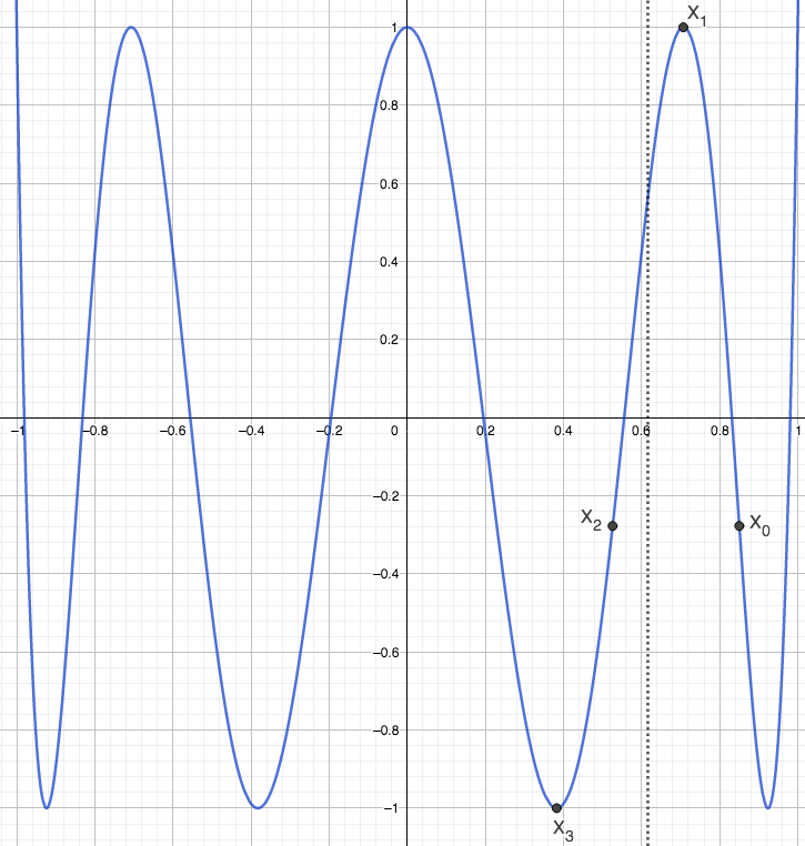
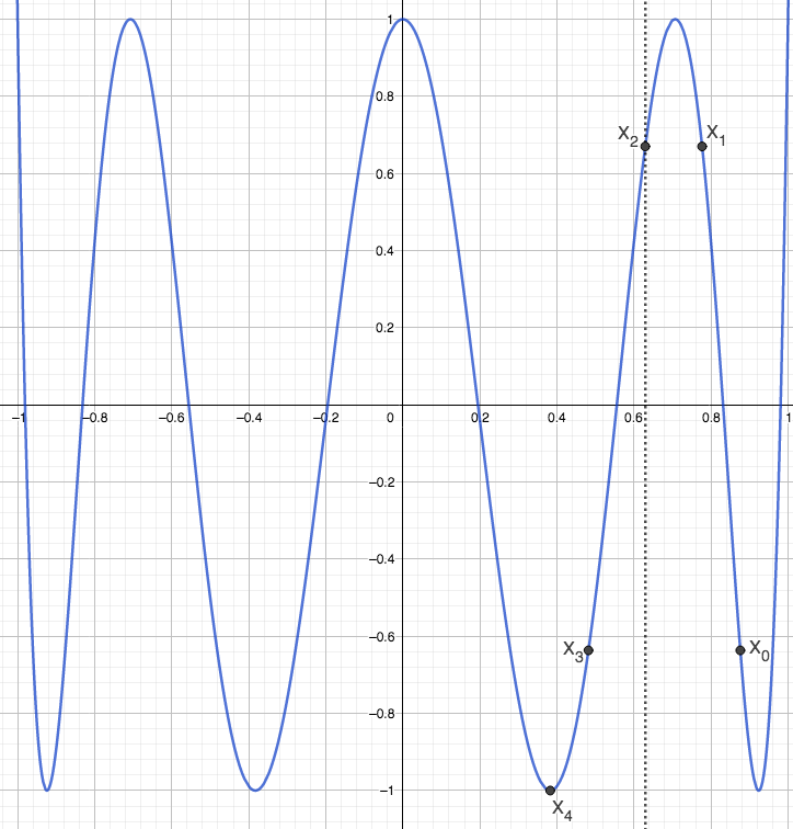
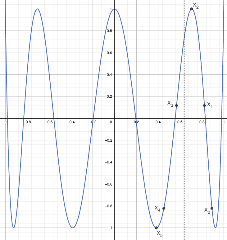
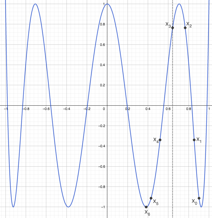
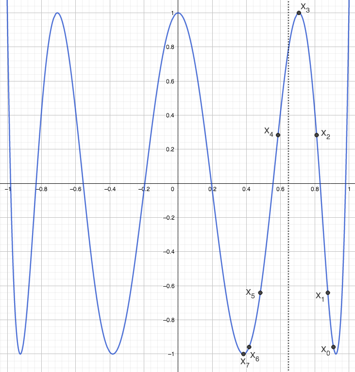
Figure 9. $T_{\kappa=8}(x)$. Solutions $\mathcal{F}_{n}$. Left to right : $\mathcal{F}_{1}\simeq 1.1874$, $\mathcal{F}_{2}\simeq 1.2331$, $\mathcal{F}_{3}\simeq 1.2589$, $\mathcal{F}_{4}\simeq 1.2749$, $\mathcal{F}_{5}\simeq 1.2853$, $\mathcal{F}_{6}\simeq 1.2922$.

Thus, we propose a generalization :

Theorem 11.2.

Fix $\kappa\geq 2$. Fix $1\leq j\leq\left\lfloor\kappa/2\right\rfloor$, $j$ even. There is a sequence $\{\mathcal{F}_{n}\}_{n=1}^{\infty}$, which depends on $\kappa$, s.t. $\{\mathcal{F}_{n}\}\subset(2\cos((j+1)\pi/\kappa),\cos((j-1)\pi/\kappa)+\cos((j+1)\pi/\kappa))\cap\bm{\Theta}_{\kappa}(\Delta)$, and $\mathcal{F}_{n}<\mathcal{F}_{n+1}<\mathcal{F}_{n+2}$, $\forall n\in\mathbb{N}^{*}$. Also, $\mathcal{F}_{2n-1}$, $\mathcal{F}_{2n}\in\bm{\Theta}_{n,\kappa}(\Delta)$, $\forall n\geq 1$, and

(11.2) $$\cos((j+1)\pi/\kappa)=:X_{n+1}<X_{n}<...<X_{1}<X_{0}<\cos((j-1)\pi/\kappa).$$

11.3. Conjecture on the limit

We conjecture :

Conjecture 11.3.

Let $\{\mathcal{F}_{n}\}$ be the sequence in Theorems 11.1 and 11.2. Then

$$\mathcal{F}_{n}\nearrow\cos((j-1)\pi/\kappa)+\cos((j+1)\pi/\kappa).$$

12. Description of the polynomial interpolation in dimension 2

This entire section is in dimension 2. In this section we adapt the linear system (LABEL:interpol_intro) to the interval $J_{2}(\kappa):=(2\cos(\frac{\pi}{\kappa}),1+\cos(\frac{\pi}{\kappa}))$. This will setup our framework behind Conjecture 1.11. In sections 13 and 14 we numerically implement the equations of this section.

Fix $\kappa\geq 2$, $n\in\mathbb{N}^{*}$. First, let $\mathcal{E}_{n},X_{0,n},...,X_{n+1,n}$ be the solutions of Propositions 7.1 and 7.2 (also Theorem 1.7). Our aim is to find the coefficients $\rho_{j_{q}\kappa}$ of $\mathbb{A}(n)=\sum_{q=1}^{N(n)}\rho_{j_{q}\kappa}(n)A_{j_{q}\kappa}$ so that a strict Mourre estimate holds on the interval $(\mathcal{E}_{n},\mathcal{E}_{n-1})$. For $n$ odd, the linear system (LABEL:interpol_intro) becomes (using notation (3.3) and (3.4) instead) :

(12.1) $$\begin{cases}G_{\kappa}^{\mathcal{E}_{n}}(X_{q,n})=0&q=0,...,(n-1)/2\\ \frac{d}{dx}G_{\kappa}^{\mathcal{E}_{n}}(X_{q,n})=0&q=1,...,(n-1)/2\\ G_{\kappa}^{\mathcal{E}_{n-1}}(X_{q,n-1})=0&q=0,...,(n-3)/2\\ \frac{d}{dx}G_{\kappa}^{\mathcal{E}_{n-1}}(X_{q,n-1})=0&q=1,...,(n-3)/2+1.\\ \end{cases}$$

This system of $2n-1$ equations has at most rank $2n-1$, but part of our conjecture is that it always has rank $2n-1$ and so one solves for $2n-1$ unknown coefficients $\rho_{j\kappa}$. For $n$ even, the linear system (LABEL:interpol_intro) becomes (using notation (3.3) and (3.4) instead) :

(12.2) $$\begin{cases}G_{\kappa}^{\mathcal{E}_{n}}(X_{q,n})=0&q=0,...,n/2-1\\ \frac{d}{dx}G_{\kappa}^{\mathcal{E}_{n}}(X_{q,n})=0&q=1,...,n/2\\ G_{\kappa}^{\mathcal{E}_{n-1}}(X_{q,n-1})=0&q=0,...,n/2-1\\ \frac{d}{dx}G_{\kappa}^{\mathcal{E}_{n-1}}(X_{q,n-1})=0&q=1,...,n/2-1.\\ \end{cases}$$

Again, this system of $2n-1$ equations has at most rank $2n-1$, but part of our conjecture is that it always has rank $2n-1$.

For the coefficients $\rho_{j_{q}\kappa}$ we will assume $\Sigma=\{\rho_{j_{1}\kappa},\rho_{j_{2}\kappa},...,\rho_{j_{2n}\kappa}\}$ and further always take the convention that $j_{1}=1$ and $\rho_{j_{1}\kappa}=\rho_{\kappa}=1$. Thus we have a system of $2n-1$ unknowns and $2n-1$ equations.

Remark 12.1.

Fix $n$ odd. By the second equation in (5.1) $g_{j\kappa}^{\mathcal{E}_{n}}(X_{1+q})=g_{j\kappa}^{\mathcal{E}_{n}}(X_{n-q})$ for $q=0,1,...,(n-1)/2$. So $G_{\kappa}^{\mathcal{E}_{n}}(X_{1+q})=G_{\kappa}^{\mathcal{E}_{n}}(X_{n-q})$ for any choice of coefficients $\rho_{j\kappa}$. And by (5.5), $G_{\kappa}^{\mathcal{E}_{n}}(X_{(n+1)/2})=\sum_{q=0}^{(n-1)/2}\omega_{q}G_{\kappa}^{\mathcal{E}_{n}}(X_{q})$. So to avoid obvious linear dependencies, we require the first line of system (12.1) only for $q=0,...,(n-1)/2$. Also a direct computation of $\frac{d}{dx}G_{\kappa}^{\mathcal{E}_{n}}(x)$ shows that $\frac{d}{dx}G_{\kappa}^{\mathcal{E}_{n}}(X_{1+q})=\frac{d}{dx}G_{\kappa}^{\mathcal{E}_{n}}(X_{n-q})$ for $q=0,1,...,(n-1)/2$ and any choice of coefficients $\rho_{j\kappa}$. And by Lemma 3.4, $\frac{d}{dx}G_{\kappa}^{\mathcal{E}_{n}}(X_{(n+1)/2})=0$ always holds. So to avoid obvious linear dependencies, we require the second line of system (12.1) only for $q=1,...,(n-1)/2$ (we don’t include $q=0$ either but that is for a separate reason based only on numerical and graphical evidence).

Remark 12.2.

Analogous remark to 12.1 holds for $n$ even.

13. Application of Polynomial Interpolation to the case $\kappa=2$ in dimension 2

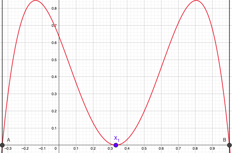
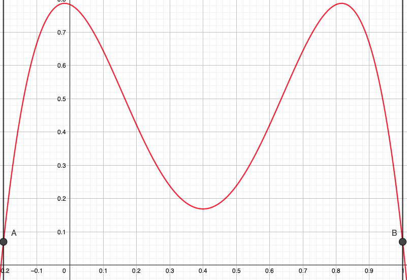
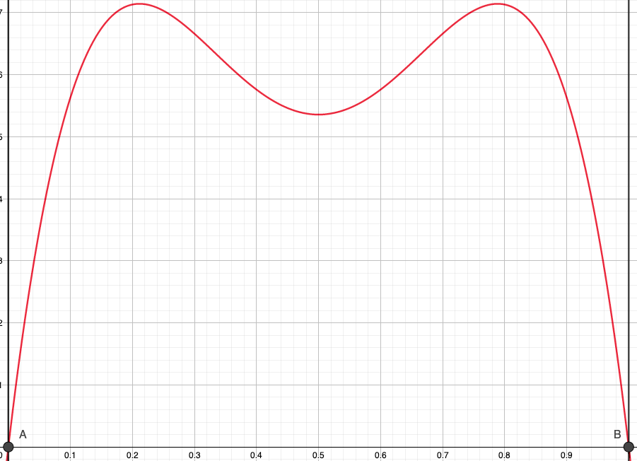
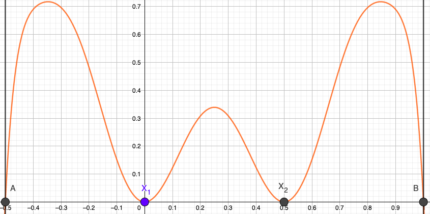
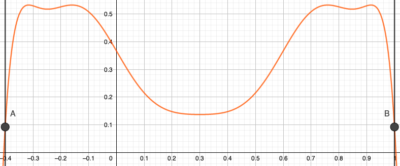
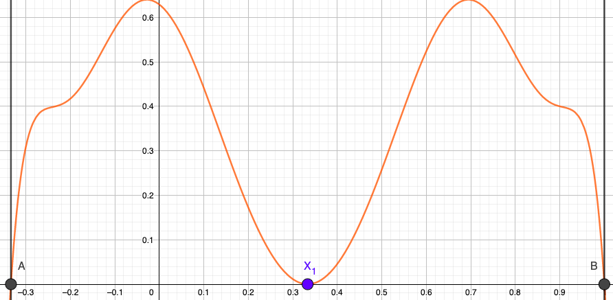
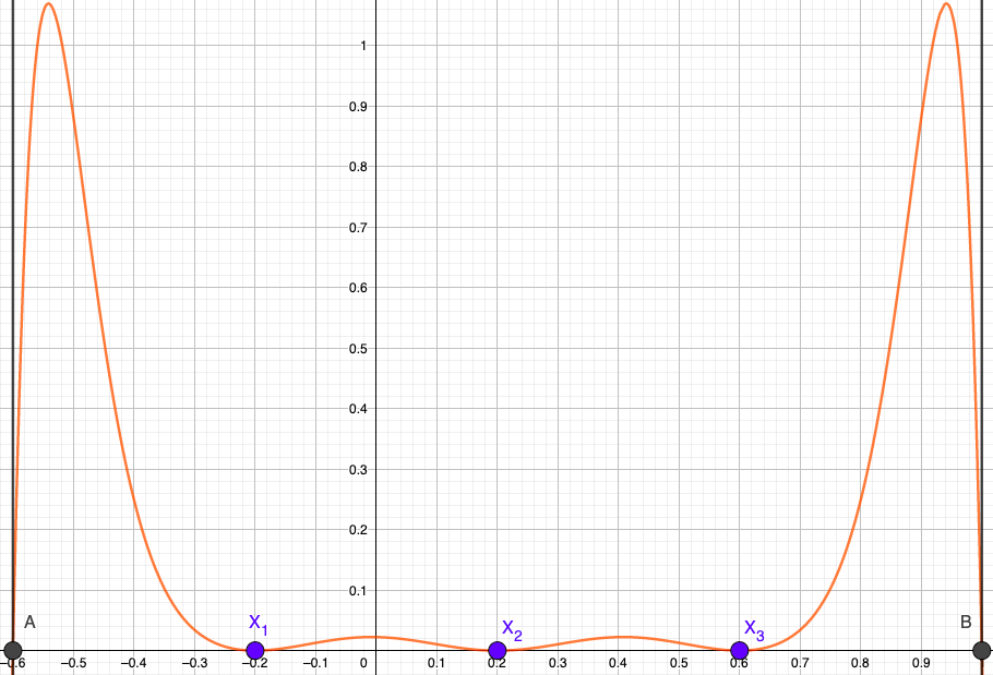
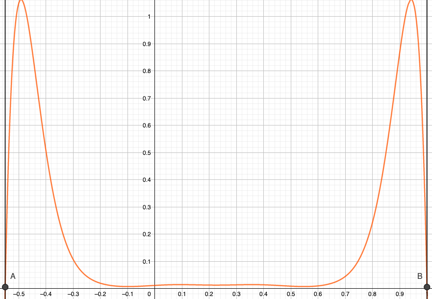
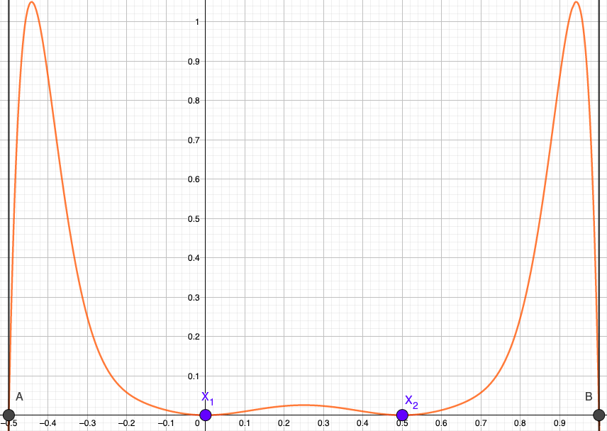
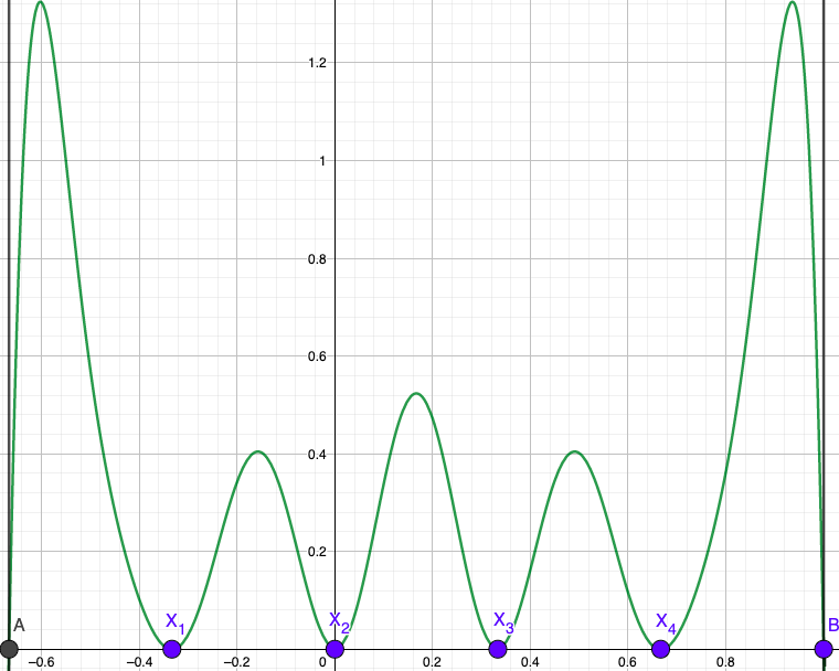
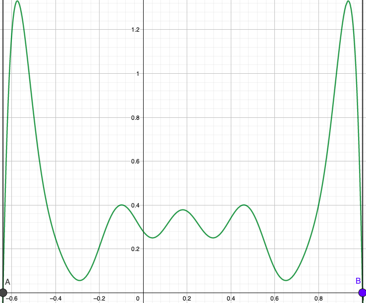
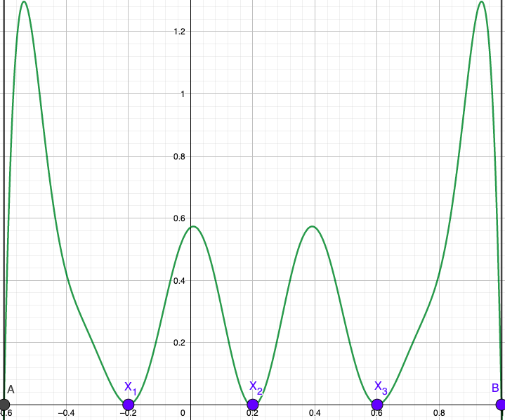
Figure 10. Plots of $G_{\kappa=2}^{E}(x)$, $x\in[E-1,1]$. Rows correspond to $n=1,2,3,4$. Left column : $E=\mathcal{E}_{n}$. Middle : some $E\in(\mathcal{E}_{n},\mathcal{E}_{n-1})$. Right column : $E=\mathcal{E}_{n-1}$.

In this section we prove Theorem 1.10 and give some graphical illustrations to justify our Conjecture 1.11 for $n=1,2,3,4$ and $\kappa=2$. See the plots of $G_{\kappa=2}^{E}(x)$ in Figure 10. In this Figure, note that in the left and right-most columns, $G_{\kappa=2}^{E}\geq 0$, whereas in the middle column, $G_{\kappa=2}^{E}(x)>0$, $\forall x\in[E-1,1]$. Throughout this section the sequence $\mathcal{E}_{n}$ referred to is that of Theorem 1.7 and Propositions 7.1 and 7.2. In the middle column of Figure 10 the values of $E$ used to illustrate $G_{\kappa=2}^{E}$ are, from to top to bottom, $E=0.8,0.6,0.45,0.36$. Subsections 13.2, 13.3, 13.4 and 13.5 detail the calculations underlying Figure 10.

Proof of Theorem 1.10.

Fix $d=\kappa=2$. It is enough to prove that $G_{\kappa}^{E}(x)=g_{2}^{E}(x)+9/14g_{4}^{E}(x)$ is such that $G_{\kappa}^{E}(x)>0$ for $E\in(2/3,1)$ and $x\in[E-1,1]$. Thanks to the computer, $G_{\kappa}^{E}(x)=-(180E/7)(x^{2}-Ex+r_{-}r_{+})(x^{2}-Ex+s_{-}s_{+})$ where

$$r_{\pm}=\frac{1}{2}\left(E\pm\frac{\sqrt{20-15E^{2}-2\sqrt{5}\sqrt{16-20E^{2}+9E^{4}}}}{\sqrt{15}}\right),\ \ s_{\pm}=\frac{1}{2}\left(E\pm\frac{\sqrt{20-15E^{2}+2\sqrt{5}\sqrt{16-20E^{2}+9E^{4}}}}{\sqrt{15}}\right),$$

which satisfy $r_{-}+r_{+}=s_{-}+s_{+}=E$ and

$$r_{-}r_{+}=\left(15E^{2}-\sqrt{5}\sqrt{16-20E^{2}+9E^{4}}-10\right)/30,\quad s_{-}s_{+}=\left(15E^{2}+\sqrt{5}\sqrt{16-20E^{2}+9E^{4}}-10\right)/30.$$

The parabola $x^{2}-Ex+r_{-}r_{+}$ has real roots iff $E\in[-2/3,2/3]$. Thus for $E\in(2/3,1)$, this parabola is strictly positive. On the other hand, the parabola $x^{2}-Ex+s_{-}s_{+}$ is strictly negative if and only if $x\in(s_{-},s_{+})$ (one checks that $s_{-},s_{+}$ are real numbers if and only if $E\in[-2,2]$). For a fixed value of $E$, we want $G_{\kappa}^{E}(x)>0$ for all $x\in[E-1,1]$. Thus we are led to solve $s_{-}\leq E-1\leq 1\leq s_{+}$ which has solutions $E\in[2/3,1]\cup[4/3,2]$. This implies the result. Note also $G_{\kappa}^{E}(x)=0$ for $E=2/3$, $x=-1/3,1/3,1$ and $E=1$, $x=0,1$, as expected. ∎

13.1. A specificity of the polynomial interpolation problem for $\kappa=2$

We have a remark that is specific to the case $\kappa=2$. Recall the definitions of $g_{j\kappa}$ and $G_{\kappa}$ given by (1.8) and (1.9) respectively. For $\kappa=2$, note that the linear span of $\{U_{j\kappa-1}(x):j\geq 1\}$ equals the linear span of $\{x^{2j-1}:j\geq 1\}$. So we can interpret the polynomial interpolation problem of finding coefficients $\rho_{j\kappa}$ such that $G_{\kappa}(\vec{x})>0$, instead as, we are looking for an odd function $f_{-}$ such that $G_{\kappa=2}(\vec{x})=\sum_{1\leq i\leq d}(1-x_{i}^{2})f_{-}(x_{i})>0$ for all $\vec{x}\in S_{E}$. We don’t know if this remark is helpful but we found it still interesting enough to mention.

Table 3 gives the inputs we need to feed linear systems (12.1) and (12.1) into the computer.

$n$	Left endpoint	Right endpoint	$\Sigma=$
1	$\mathcal{E}_{1}=\frac{2}{3}$, $X_{1}=\mathcal{E}_{1}/2=\frac{1}{3}$	$\mathcal{E}_{0}=1$	{2,4}
2	$\mathcal{E}_{2}=\frac{1}{2}$, $X_{1}=0$, $X_{2}=\frac{1}{2}$	$\mathcal{E}_{1}=\frac{2}{3}$, $X_{1}=\frac{1}{3}$	$\{2,4,6,10\}$
3	$\mathcal{E}_{3}=\frac{2}{5}$, $X_{1}=-\frac{1}{5}$, $X_{2}=\frac{1}{5}$, $X_{3}=\frac{3}{5}$	$\mathcal{E}_{2}=\frac{1}{2}$, $X_{1}=0$, $X_{2}=\frac{1}{2}$	$\{2,4,6,8,10,12\}$
4	$\mathcal{E}_{4}=\frac{1}{3}$, $X_{1}=-\frac{1}{3}$, $X_{2}=0$, $X_{3}=\frac{1}{3}$, $X_{4}=\frac{2}{3}$	$\mathcal{E}_{3}=\frac{2}{5}$, $X_{1}=-\frac{1}{5}$, $X_{2}=\frac{1}{5}$, $X_{3}=\frac{3}{5}$	$\{2,4,6,8,10,12,14,20\}$

Table 3. Data to setup polynomial interpolation on $(\mathcal{E}_{n},\mathcal{E}_{n-1})$. $\kappa=2$. $d=2$.

13.2. $1st$ band ($n=1$)

By Lemma 1.4, $\mathcal{E}_{0}\in\bm{\Theta}_{0,\kappa}(\Delta)$ and $G_{\kappa}^{\mathcal{E}_{0}}(\mathcal{E}_{0}-1)=0$ is always true. By Lemma 3.4, $\frac{d}{dx}G_{\kappa}^{\mathcal{E}_{1}}(X_{1})=0$ is always true. So these are fake constraints. Then we compute

$$M=\begin{bmatrix}g_{2}^{\mathcal{E}_{1}}(\mathcal{E}_{1}-1)&g_{4}^{\mathcal{E}_{1}}(\mathcal{E}_{1}-1)\end{bmatrix}=\begin{bmatrix}-\frac{16}{27}&\frac{224}{243}\end{bmatrix},\quad\rho=\begin{bmatrix}1,&\rho_{4}\end{bmatrix}^{T}.\quad M\rho=0\Rightarrow\rho_{4}=9/14.$$

13.3. $2nd$ band ($n=2$)

Matrix $M$ equals

$$\begin{bmatrix}g_{2}^{\mathcal{E}_{2}}(\mathcal{E}_{2}-1)&g_{4}^{\mathcal{E}_{2}}(\mathcal{E}_{2}-1)&g_{6}^{\mathcal{E}_{2}}(\mathcal{E}_{2}-1)&g_{10}^{\mathcal{E}_{2}}(\mathcal{E}_{2}-1)\\[5.0pt] \frac{d}{dx}g_{2}^{\mathcal{E}_{2}}(X_{1})&\frac{d}{dx}g_{4}^{\mathcal{E}_{2}}(X_{1})&\frac{d}{dx}g_{6}^{\mathcal{E}_{2}}(X_{1})&\frac{d}{dx}g_{10}^{\mathcal{E}_{2}}(X_{1})\\[5.0pt] g_{2}^{\mathcal{E}_{1}}(\mathcal{E}_{1}-1)&g_{4}^{\mathcal{E}_{1}}(\mathcal{E}_{1}-1)&g_{6}^{\mathcal{E}_{1}}(\mathcal{E}_{1}-1)&g_{10}^{\mathcal{E}_{1}}(\mathcal{E}_{1}-1)\\[5.0pt] \end{bmatrix}=\begin{bmatrix}-3/4&3/4&0&3/4\\[5.0pt] 3/2&-13/2&12&9/2\\[5.0pt] -\frac{16}{27}&\frac{224}{243}&-\frac{1840}{2187}&\frac{42416}{177147}\\[5.0pt] \end{bmatrix}.$$

$$M\rho=0\Rightarrow\rho=[1,\rho_{4},\rho_{6},\rho_{10}]^{T}=[1,598/787,464/2361,189/787]^{T}\simeq[1,0.7598,0.1965,0.2401]^{T}.$$

13.4. $3rd$ band ($n=3$)

Matrix $M$ equals

$$\begin{bmatrix}g_{2}^{\mathcal{E}_{3}}(\mathcal{E}_{3}-1)&...&g_{12}^{\mathcal{E}_{3}}(\mathcal{E}_{3}-1)\\[5.0pt] g_{2}^{\mathcal{E}_{3}}(X_{1})&...&g_{12}^{\mathcal{E}_{3}}(X_{1})\\[5.0pt] \frac{d}{dx}g_{2}^{\mathcal{E}_{3}}(X_{1})&...&\frac{d}{dx}g_{12}^{\mathcal{E}_{3}}(X_{1})\\[5.0pt] g_{2}^{\mathcal{E}_{2}}(\mathcal{E}_{2}-1)&...&g_{12}^{\mathcal{E}_{2}}(\mathcal{E}_{2}-1)\\[5.0pt] \frac{d}{dx}g_{2}^{\mathcal{E}_{2}}(X_{1})&...&\frac{d}{dx}g_{12}^{\mathcal{E}_{2}}(X_{1})\end{bmatrix}=\begin{bmatrix}-\frac{96}{125}&\frac{1344}{3125}&\frac{41184}{78125}&-\frac{1416576}{1953125}&-\frac{5907936}{48828125}&\frac{968071104}{1220703125}\\[5.0pt] \frac{48}{125}&\frac{864}{3125}&-\frac{112752}{78125}&\frac{3328704}{1953125}&-\frac{37319952}{48828125}&-\frac{174668256}{1220703125}\\[5.0pt] \frac{48}{25}&-\frac{32}{5}&\frac{93072}{15625}&\frac{357824}{78125}&-\frac{139067664}{9765625}&\frac{485868192}{48828125}\\[5.0pt] -3/4&3/4&0&-3/4&3/4&0\\[5.0pt] 3/2&-13/2&12&-23/2&9/2&0\end{bmatrix}.$$

The system $M\rho=0$ has the solution $\rho=[\rho_{2},\rho_{4},\rho_{6},\rho_{8},\rho_{10},\rho_{12}]^{T}$ equals

$$\bigg{[}1,\frac{879159}{627154},\frac{368515}{313577},\frac{419505}{627154},\frac{83750}{313577},\frac{1146875}{14424542}\bigg{]}^{T}\simeq[1,1.4018,1.1751,0.6689,0.2670,0.0795]^{T}.$$

$M$ has rank 5, which is the number of unknown parameters in $\rho$.

13.5. $4th$ band $(n=4)$

Matrix $M$ is too large to write out. $M\rho=0\Rightarrow[\rho_{2},\rho_{4},\rho_{6},\rho_{8},\rho_{10},\rho_{12},\rho_{14},\rho_{20}]^{T}=$

$$\Big{[}1,\frac{91312852394687883497633}{60342582799484620292280},\frac{2214634471921172327027}{1508564569987115507307},\frac{7972149322756114102612}{7542822849935577536535},\frac{1480399911203653752057}{2514274283311859178845},$$

$$\quad\frac{305875819949113732527}{1149382529513992767472},\frac{6549161566940548875}{71836408094624547967},-\frac{16094965193651953125}{8045677706597949372304}\Big{]}^{T}$$

$$\simeq[1,1.5132,1.4680,1.0569,0.5887,0.2661,0.0911,-0.0020]^{T}.$$

$M$ has rank 7, which corresponds to the number of unknown parameters in $\rho$.

Remark 13.1.

We check the linear dependencies between the rows of $M$ using linear regression (Python’s statsmodels for example) and assess based on the $R^{2}$ among various statistics.

14. Application of Polynomial Interpolation for $\kappa=3$ in dimension 2

In this section we give graphical illustrations to justify our Conjecture 1.11 for $n=1,2,3,4$ and $\kappa=3$. See the plots of $G_{\kappa=3}^{E}(x)$ in Figure 11. In this Figure, note that in the left and right-most columns, $G_{\kappa=3}^{E}\geq 0$, whereas in the middle column, $G_{\kappa=3}^{E}(x)>0$, $\forall x\in[E-1,1]$. Throughout this section the sequence $\mathcal{E}_{n}$ referred to is that of Theorem 1.7 and Propositions 7.1 and 7.2. In the middle column of Figure 11 the values of $E$ used to illustrate $G_{\kappa=3}^{E}$ are, from to top to bottom, $E=1.4,1.26,1.2,1.15$. Subsections 13.2, 13.3, 13.4 and 13.5 detail the calculations underlying Figure 11.

Table 4 gives the inputs we need to feed linear systems (12.1) and (12.1) into the computer.

$n$	Left endpoint	Right endpoint	$\Sigma=$
1	$\mathcal{E}_{1}=\frac{5+3\sqrt{2}}{7}\simeq 1.3203$, $X_{1}=\frac{5+3\sqrt{2}}{14}$	$\mathcal{E}_{0}=1+\cos(\frac{\pi}{3})=\frac{3}{2}$	$\{3,6\}$
2	$\mathcal{E}_{2}=(9+\sqrt{33})/12\simeq 1.2287$, $X_{1}=1/2$, $X_{2}=(3+\sqrt{33})/12$	$=$ left endpt data of $n=1$	$\{3,6,9,18\}$
3	$\mathcal{E}_{3}\simeq 1.1737$, $X_{1}\simeq 0.4077$, $X_{2}=\mathcal{E}_{3}/2$, $X_{3}=\mathcal{E}_{3}-X_{1}$.	$=$ left endpt data of $n=2$	$\{3,6,9,12,15,18\}$
4	$\mathcal{E}_{4}\simeq 1.1375$, $X_{1}\simeq 0.3484$, $X_{2}=1/2$, $X_{3}=\mathcal{E}_{4}-X_{2}$, $X_{4}=\mathcal{E}_{4}-X_{1}$	$=$ left endpt data of $n=3$	$\{3,6,9,12,15,18,21,36\}$

Table 4. Data to setup polynomial interpolation on $(\mathcal{E}_{n},\mathcal{E}_{n-1})$. $\kappa=3$. $d=2$.

14.1. $1st$ band $(n=1)$

$M\rho=0\Rightarrow\rho=[\rho_{3},\rho_{6}]^{T}=[1,\frac{170-81\sqrt{2}}{92}]^{T}\simeq[1,0.6027]^{T}$.

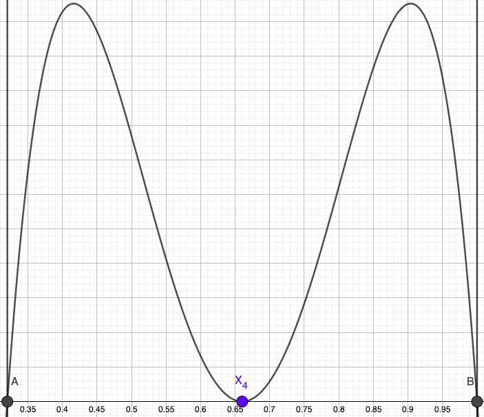
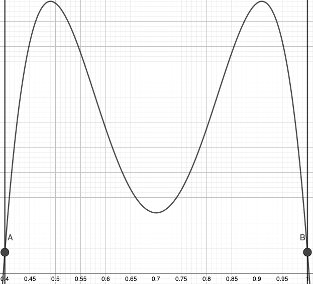
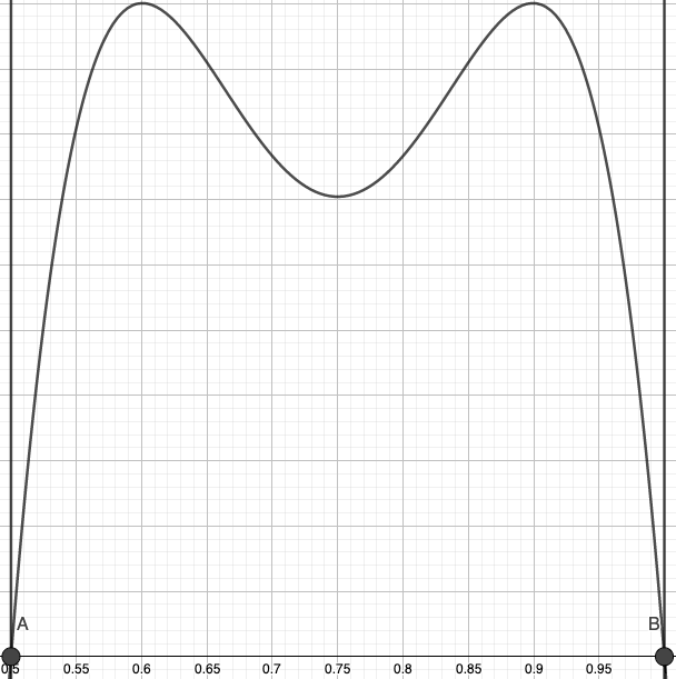
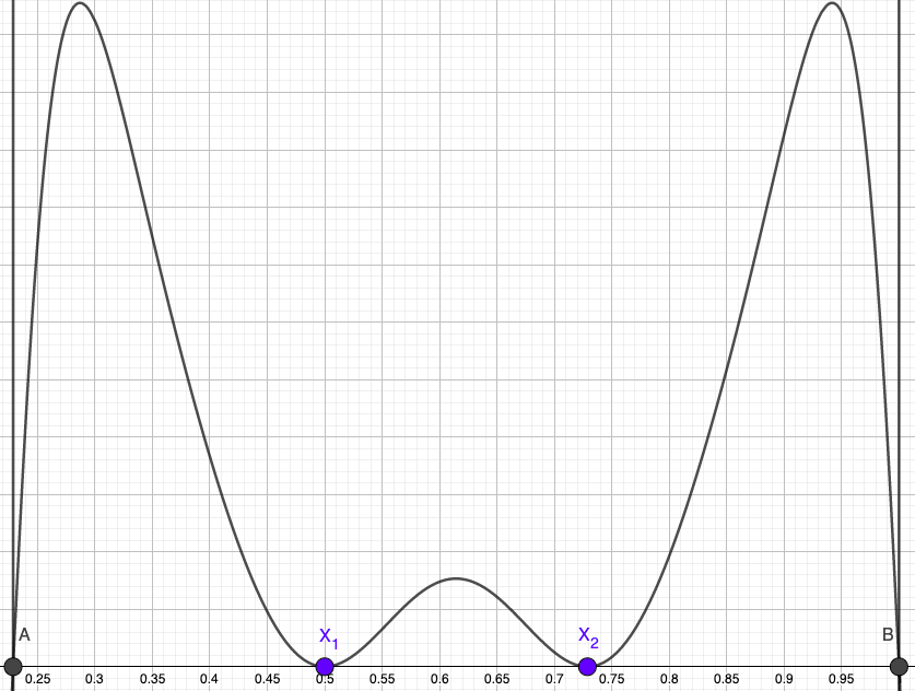
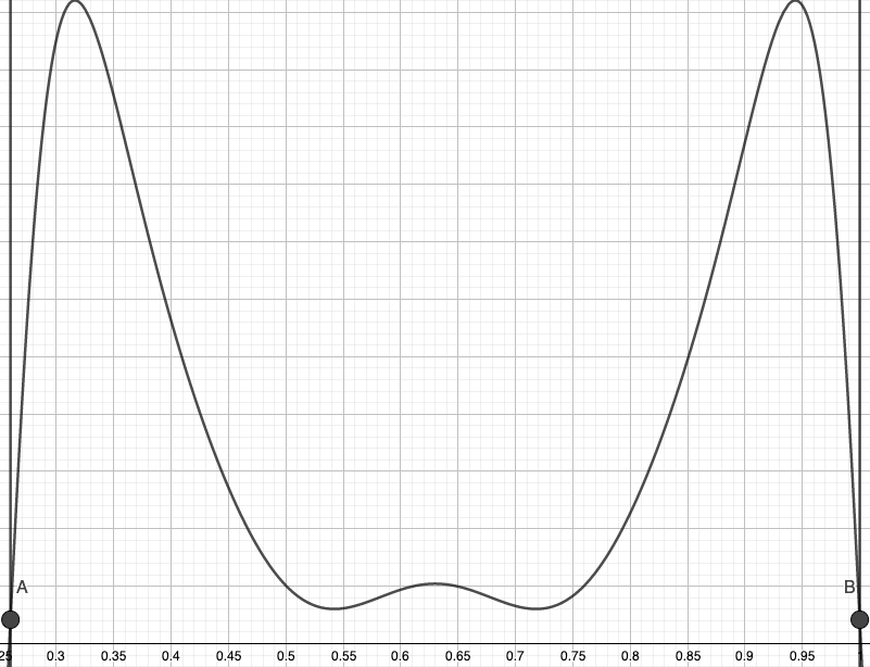
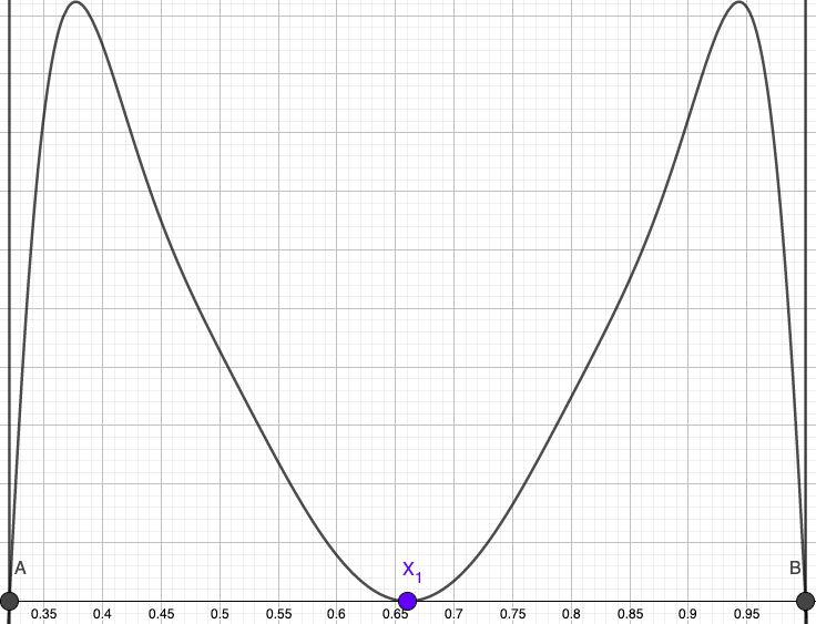
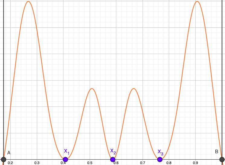
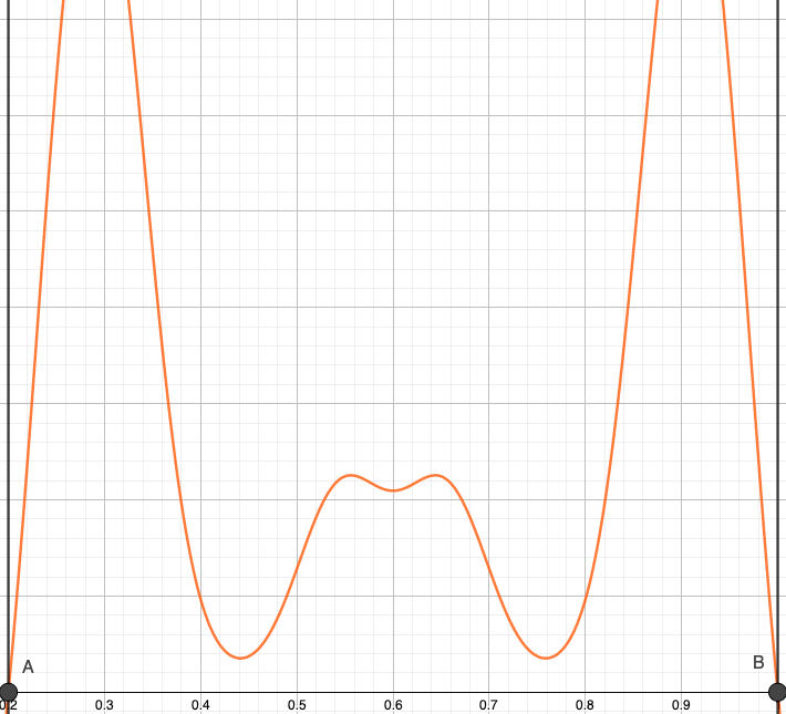
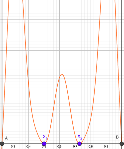
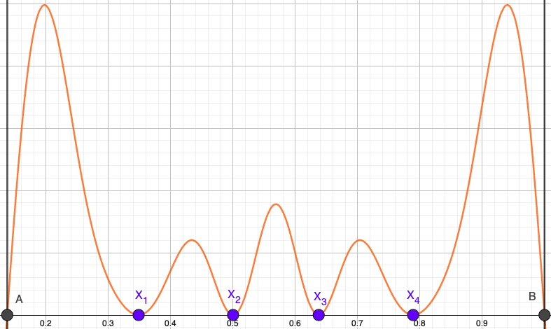
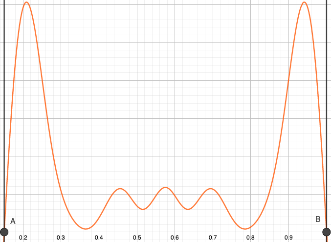
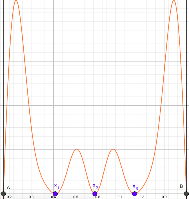
Figure 11. Plots of $G_{\kappa=3}^{E}(x)$, $x\in[E-1,1]$. Rows correspond to $n=1,2,3,4$. Left column : $E=\mathcal{E}_{n}$. Middle : some $E\in(\mathcal{E}_{n},\mathcal{E}_{n-1})$. Right column : $E=\mathcal{E}_{n-1}$.

14.2. $2nd$ band ($n=2$)

$M\rho=0\Rightarrow\rho=[\rho_{3},\rho_{6},\rho_{9},\rho_{18}]^{T}\simeq[1,0.8854,0.2861,-0.0452]^{T}.$

14.3. $3rd$ band $(n=3)$

$X_{2}=\mathcal{E}_{3}/2$ and $T_{3}(\mathcal{E}_{3}-1)=T_{3}(\mathcal{E}_{3}-X_{1})$, $T_{3}(X_{1})=T_{3}(\mathcal{E}_{3}/2)$. Applying (2.2) leads to

$$\begin{cases}4\left((\mathcal{E}_{3}-1)^{2}+(\mathcal{E}_{3}-1)(\mathcal{E}_{3}-X_{1})+(\mathcal{E}_{3}-X_{1})^{2}\right)=3\\ 4\left(X_{1}^{2}+X_{1}\mathcal{E}_{3}/2+\mathcal{E}_{3}^{2}/4\right)=3.\end{cases}$$

Subtract the equations to get $X_{1}=(3\mathcal{E}_{3}-11\mathcal{E}_{3}^{2}/4-1)(1-7\mathcal{E}_{3}/2)^{-1}$. This leads to

(14.1) $$\mathcal{E}_{3}=\frac{199}{494}+\frac{\sqrt{49149+247t+2223s}}{494\sqrt{3}}+\frac{1}{2}\sqrt{\frac{32766}{61009}-\frac{t}{741}-\frac{3s}{247}+\frac{4340412\sqrt{3}}{61009\sqrt{49149+247t+2223s}}},$$

where $t=\sqrt[3]{2625129-139968\sqrt{327}}$ and $s=\sqrt[3]{3601+192\sqrt{327}}$. So $\mathcal{E}_{3}\simeq 1.1737$. On the other hand, $\mathcal{E}_{3}=(X_{1}-11X_{1}^{2}+37/4)(3+9X_{1})^{-1}$. So

$$X_{1}=-\frac{73}{494}+\frac{\sqrt{2129040+247q+17784r}}{1976\sqrt{3}}-\frac{1}{2}\sqrt{\frac{88710}{61009}-\frac{q}{11856}-\frac{3r}{494}+\frac{5651424}{61009}\frac{\sqrt{3}}{\sqrt{2129040+247q+17784r}}}.$$

$q=\sqrt[3]{569651470848-1240676352\sqrt{327}}$, and $r=\sqrt[3]{1526201+3324\sqrt{327}}$. So $X_{1}\simeq 0.4077$. The minimal polynomials of $\mathcal{E}_{3}$ is

$$mp(E)=247E^{4}-398E^{3}+141E^{2}-20E+4,$$

Also, $X_{3}=-(\mathcal{E}_{3}-1)/2+\sqrt{3}\sqrt{1-(\mathcal{E}_{3}-1)^{2}}/2\simeq 0.76598$. Next we suppose $\Sigma=[3,6,9,12,15,18]$. Python says the solution to $M\rho=0$ is
$\rho=[\rho_{3},\rho_{6},\rho_{9},\rho_{12},\rho_{15},\rho_{18}]^{T}\simeq[1,1.38266,1.09831,0.56967,0.18700,0.03160]^{T}.$

14.4. $4th$ band ($n=4$)

$X_{2}=1/2$, and $T_{3}(\mathcal{E}_{4}-1)=T_{3}(\mathcal{E}_{4}-X_{1})$ and $T_{3}(X_{1})=T_{3}(\mathcal{E}_{4}-1/2)$. Thus :

$$\begin{cases}(\mathcal{E}_{4}-1)^{2}+(\mathcal{E}_{4}-1)(\mathcal{E}_{4}-X_{1})+(\mathcal{E}_{4}-X_{1})^{2}=\frac{3}{4}&\\ X_{1}^{2}+X_{1}(\mathcal{E}_{4}-\frac{1}{2})+(\mathcal{E}_{4}-\frac{1}{2})^{2}=\frac{3}{4}&\end{cases}\Leftrightarrow\begin{cases}X_{1}^{2}+X_{1}(\mathcal{E}_{4}-\frac{1}{2})+(\mathcal{E}_{4}-\frac{1}{2})^{2}=\frac{3}{4}&\\ X_{1}=\frac{8\mathcal{E}_{4}^{2}-8\mathcal{E}_{4}+3}{16\mathcal{E}_{4}-6}.&\end{cases}$$

Technically speaking there are 4 solutions for $\mathcal{E}_{4}\simeq 0,0.23,0.44,1.13$. Given the context we infer

(14.2) $$\mathcal{E}_{4}=\frac{17}{28}+\frac{\sqrt{58}}{14}\cos\left(\frac{1}{3}\arctan\left(\frac{21\sqrt{687}}{691}\right)\right)\simeq 1.1375.$$

The minimal polynomial of $\mathcal{E}_{4}$ is $mp(E)=224E^{3}-408E^{2}+198E-27.$ To solve for $X_{1}$, eliminate the $\mathcal{E}_{4}^{2}$ in the system. One gets $\mathcal{E}_{4}=(-8X_{1}^{2}+10X_{1}+7)/(24X_{1})$. Technically there are 4 possibilities for $X_{1}\simeq-0.70,-0.5,0.34,0.89$. Given the context we infer

(14.3) $$X_{1} =\frac{5}{28}-\frac{\sqrt{43}}{14}\left(\sqrt{3}\sin(\beta)-\cos(\beta)\right)\simeq 0.3484.$$

where $\beta=\frac{1}{3}\arctan\left(\frac{147\sqrt{687}}{2347}\right)$. The minimal polynomial of $X_{1}$ is $mp(X)=224X^{3}-120X^{2}-126X+49$. The minimal polynomial of $X_{3}=\mathcal{E}_{4}-X_{2}\simeq 0.6375$ is $mp(X)=112X^{3}-36X^{2}-21X-1$. Determining the minimal polynomial of $X_{4}=\mathcal{E}_{4}-X_{1}\simeq 0.7890$ didn’t seem worth the effort. Next we suppose $\Sigma=[3,6,9,12,15,18,21,36]$. We fill the matrix $M$ with floats (exact numbers are getting complicated). Python says the solution to $M\rho=0$ is $[\rho_{3},\rho_{6},\rho_{9},\rho_{12},\rho_{15},\rho_{18},\rho_{21},\rho_{36}]^{T}\simeq[1,1.48690,1.34705,0.86282,0.39635,0.12308,0.02043,-0.00012]^{T}.$ On the other hand it seems $\Sigma=[3,6,9,12,15,18,21,3j]$ is not valid for $j=8,9,10,11$.

15. How to choose the correct indices $\Sigma=\{j_{1}\kappa,j_{2}\kappa,...,j_{2n}\kappa\}$ ?

This section is in dimension 2. In this section our message is : certainly not any $2n$-linear combination of the form (1.6) works on the interval $J_{2}(\kappa):=(2\cos(\pi/\kappa),1+\cos(\pi/\kappa))$, but many do work.

$\bullet$ For $\kappa=2$, $n=2$ : let us assume instead $\Sigma=\{2,4,8,16\}$. Then we find coefficients

$$\rho=[\rho_{2},\rho_{4},\rho_{8},\rho_{16}]^{T}=\bigg{[}1,\frac{3975779}{5332320},-\frac{2837741}{10664640},-\frac{13851}{1184960}\bigg{]}^{T}\simeq[1,0.7456,-0.2660,-0.0116]^{T}.$$

This gives a valid combination. We have additionally checked that the combinations $\Sigma=\{2,4,8,2j\}$ are also valid, for $j=5,6,8$, whereas $\Sigma=\{2,4,6,8\}$, $\{4,6,8,10\}$ and $\{2,6,8,10\}$ are not valid. Figure 12 has 2 examples of valid solutions and 2 examples of invalid solutions, on the interval $(\mathcal{E}_{2},\mathcal{E}_{1})=(1/2,2/3)$.

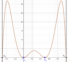
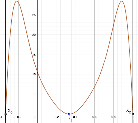
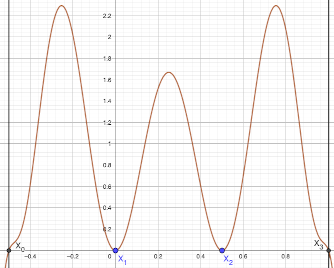
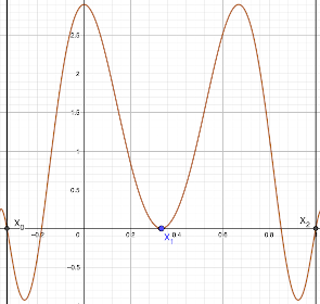
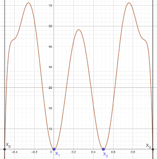
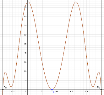
Figure 12. Plot of $G_{\kappa=2}^{E}(x)$, $x\in[E-1,1]$. Top row : $\Sigma=\{2,4,6,8\}$ for first 2 graphs and $\Sigma=\{2,4,6,12\}$ for last 2 graphs. Bottom row : $\Sigma=\{2,6,8,10\}$ for first 2 graphs and $\Sigma=\{2,4,10,14\}$ for last 2 graphs. In all cases, Left : $E=\mathcal{E}_{2}(\kappa=2)=1/2$. Right : $E=\mathcal{E}_{1}(\kappa=2)=2/3$.

$\bullet$ For $\kappa=3$, $n=2$ : other combinations of $\Sigma$’s are valid. For instance $\Sigma=\{3,6,9,21\}$ is also valid, yielding positivity on the same band, but $\Sigma=\{3,6,9,12\}$ and $\{3,6,9,15\}$ are not valid.

16. Conjecture for the interval $J_{3}(\kappa):=(1+\cos(2\pi/\kappa),2\cos(\pi/\kappa))$

In this section we give evidence for Conjecture 1.12. We only do $\kappa=3,4$.

$\kappa$	$\beta,\beta^{\prime}$	proved in [GM2]	Conjecture based on Table 6 (improvement)
3	$\beta=\frac{1}{2}(\frac{1}{2}(5-\sqrt{7}))^{1/2}\simeq 0.5425$	$(\beta,1)\subset\bm{\mu}_{\kappa}(\Delta)$	$J_{3}=(1/2,1)\subset\bm{\mu}_{\kappa}(\Delta)$
4	$\beta^{\prime}=(\frac{3}{2}-\frac{1}{\sqrt{5}})^{1/2}\simeq 1.0261$	$(\beta^{\prime},\sqrt{2})\subset\bm{\mu}_{\kappa}(\Delta)$	$J_{3}=(1,\sqrt{2})\subset\bm{\mu}_{\kappa}(\Delta)$

Table 5. Sets $\subset\bm{\mu}_{\kappa}(\Delta)$. $d=2$. Proved in [GM2] vs. conjectured

Intervals $\subset\bm{\mu}_{\kappa}(\Delta)$. $\kappa=3$	Intervals $\subset\bm{\mu}_{\kappa}(\Delta)$. $\kappa=4$
$(0.518,0.64):\rho=(1,0.6)$	$(1.00209,1.049):\rho=(1,0,0,0.8331)$
$(0.5082,0.54):\rho=(1,1,0.8)$	$(1.0011,1.096):\rho=(1,0.3,0,-0.1,0,0.465)$
$(0.5037,0.5087):\rho=(1,0.926,0.5,2.5)$
Union of intervals : $(0.5037,0.64)$	Union of intervals : $(1.0011,1.096)$

Table 6. Sets $\subset\bm{\mu}_{\kappa}(\Delta)$. $d=2$. $\rho$ of the form : $\rho=(\rho_{\kappa},\rho_{2\kappa},\rho_{3\kappa},....)$

The coefficients $\rho=(\rho_{j\kappa})$ in Table 6 were found just by fiddling around with the coefficients and the graphs (we don’t know how to cast this problem into polynomial interpolation).

17. $\left(9-\sqrt{33})/12,2/7\right)$ is a band of a.c. spectrum for $\kappa=3$ in dimension 2 : evidence

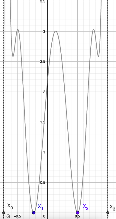
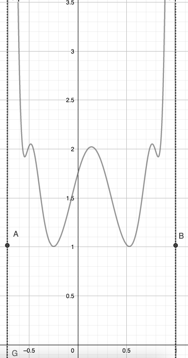
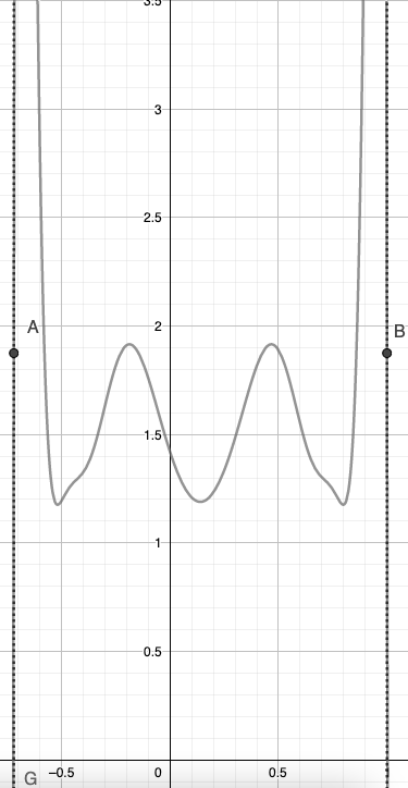
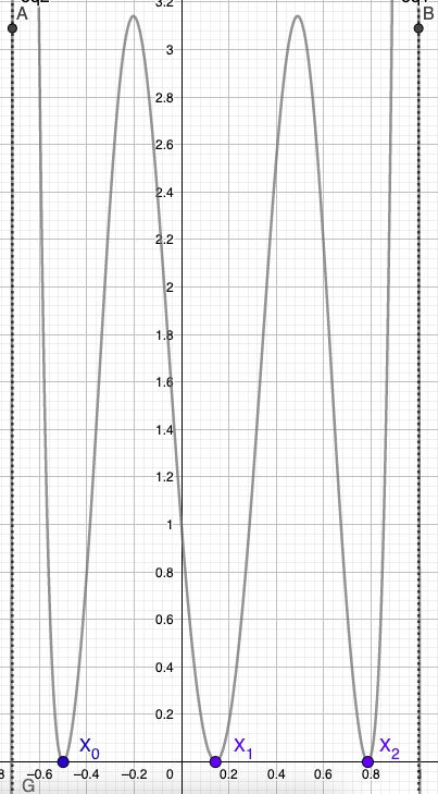
Figure 13. $G_{\kappa=3}^{E}(x)$, $x\in[E-1,1]$. From left to right: $E=(9-\sqrt{33})/12\simeq 0.2713$, $E=0.276$, $E=0.28$, $E=2/7\simeq 0.2857$. $G_{\kappa=3}^{E}(x)>0$ in the 2 middle pictures, but not in the other two.

The 2 energies $(9-\sqrt{33})/12$ and $2/7$ belong to $\bm{\Theta}_{1,\kappa=3}(\Delta)$ as per Table 2. Python says the solution to $M\rho=0$ is $[\rho_{3},\rho_{6},\rho_{9},\rho_{12},\rho_{15}]^{T}\simeq[-2.1648\cdot t,-7.2577\cdot t,22.5984\cdot t,3.3111\cdot t,t]^{T},\ t\in\mathbb{R}$. $G_{\kappa=3}^{E}(x)$ is plotted in Figure 13 for $t=1$.

18. Numerical evidence for a band of a.c. spectrum for $\kappa=8$ in dimension 2

Fix $\kappa=8$, $d=2$. We see from Table 7 that $(0,1+\cos(\frac{3\pi}{8}))$ was identified as a gap in our prior work. Can we find a linear combination of conjugate operators that gives positivity on an interval to reduce this gap ? We look for a band that is adjacent and to the left of $\mathcal{H}_{0}:=1+\cos(\frac{3\pi}{8})$. Our numerical calculations suggest that $\exists\mathcal{H}_{1}$ such that $(\mathcal{H}_{1},\mathcal{H}_{0})\subset\bm{\mu}_{\kappa=8}(\Delta)$, but the point is that the system of linear equations (LABEL:interpol_intro) is underspecified.

To determine the nearest threshold to the right of $\mathcal{H}_{0}$, let’s call it $\mathcal{H}_{1}$. We assume $\mathcal{H}_{1}\in\bm{\Theta}_{1,\kappa}(\Delta)$. So $\omega_{0}g_{j\kappa}^{\mathcal{H}_{1}}(X_{1})=g_{j\kappa}^{\mathcal{H}_{1}}(X_{0})$, $\forall j\in\mathbb{N}^{*}$. To solve this equation, we follow the path of Ansatz (1) in the context of (4.4) : we make the assumption that $X_{0}=\mathcal{H}_{1}-1$ and $T_{8}(X_{0})=T_{8}(X_{1})=T_{8}(\mathcal{H}_{1}-X_{1})$. Thus we have a system of 3 equations, 3 unknowns ($\mathcal{H}_{1}$, $X_{0}$, $X_{1}$). There are many solutions to this system; we will focus on the one where

$$\mathcal{H}_{1}=\frac{1}{2}\left(\sqrt{2}+2\sqrt{\sqrt{2}-1}\right)\simeq 1.3507,\quad X_{1}=\frac{2}{5}+\frac{1}{5}\mathcal{H}_{1}+\frac{2}{5}\mathcal{H}_{1}^{2}-\frac{2}{5}\mathcal{H}_{1}^{3}\simeq 0.4142.$$

We then compute $\omega_{0}=g_{\kappa}^{\mathcal{H}_{1}}(X_{0})/g_{\kappa}^{\mathcal{H}_{1}}(X_{1})\simeq-0.7427<0$, which means that $\mathcal{H}_{1}\in\bm{\Theta}_{1,8}(\Delta)$. Next, we assume a linear combination of the form $\mathbb{A}=A_{8}+\rho_{16}A_{16}+\rho_{24}A_{24}$. So $G_{8}^{E}(x)=g_{8}^{E}(x)+\rho_{16}g_{16}^{E}(x)+\rho_{24}g_{24}^{E}(x)$. To determine $\rho_{16}$ and $\rho_{24}$ we perform polynomial interpolation with the following only constraint : $G_{8}^{\mathcal{H}_{1}}(X_{0})=0$. Note that by construction this constraint is equivalent to $G_{8}^{\mathcal{H}_{1}}(X_{1})=0$ and $G_{8}^{\mathcal{H}_{1}}(\mathcal{H}_{1}-X_{1})=0$. Also, by Lemma 1.4, $G_{8}^{\mathcal{H}_{0}}(\mathcal{H}_{0}-1)=0$ always holds. The interesting difference here is that we also have $[g_{8j_{1}}^{\mathcal{H}_{1}}(X_{0}),\frac{d}{dx}g_{8j_{2}}^{\mathcal{H}_{1}}(X_{1})]=0$ for all $j_{1},j_{2}\in\mathbb{N}^{*}$ (expand and use the fact $T_{8}(X_{0})=T_{8}(X_{1})=T_{8}(\mathcal{H}_{1}-X_{1})$ and $(x^{2}-1)\frac{d}{dx}U_{j\kappa-1}(x)=j\kappa T_{j\kappa}(x)-xU_{j\kappa-1}(x)$). It is not clear to us if this means that $\exists\lambda$ such that $g_{8j}^{\mathcal{H}_{1}}(X_{0})=\lambda\frac{d}{dx}g_{8j}^{\mathcal{H}_{1}}(X_{1})$ for all $j\in\mathbb{N}^{*}$. It seems that the constraint $\frac{d}{dx}G_{8}^{\mathcal{H}_{1}}(X_{1})=0$ is redundant. One also checks that $\frac{d}{dx}G_{8}^{\mathcal{H}_{1}}(X_{2})=0$. Coming back to our interpolation problem, $G_{8}^{\mathcal{H}_{1}}(X_{0})=0$ leads to

$$\rho_{16}=-\left(g_{8}^{\mathcal{H}_{1}}(X_{0})+\rho_{24}g_{24}^{\mathcal{H}_{1}}(X_{0})\right)/g_{16}^{\mathcal{H}_{1}}(X_{0})=-\left(U_{7}(\mathcal{H}_{1}-1)+\rho_{24}U_{23}(\mathcal{H}_{1}-1)\right)/U_{15}(\mathcal{H}_{1}-1).$$

The point is that here we have 1 degree of freedom, namely $\rho_{24}$. Numerically, $\rho_{16}\simeq 0.51952+1.40530\rho_{24}$. Graphically, it appears that $G_{8}^{E}(x)>0$ for $E\in(\mathcal{H}_{1},\mathcal{H}_{0})$ and $\rho_{24}$ roughly in $(-0.36,-0.51)$.

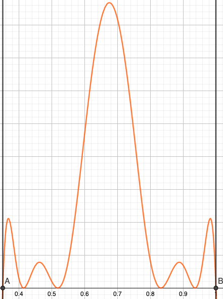
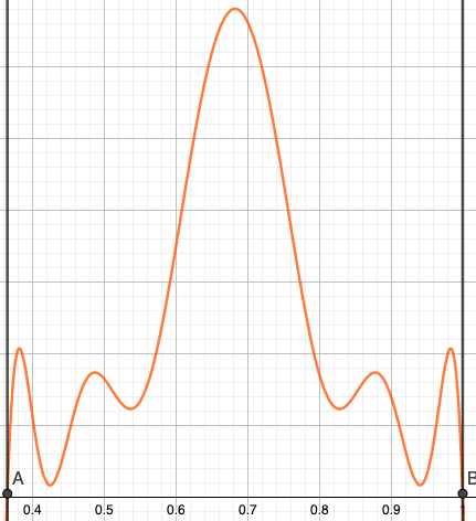
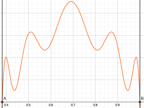
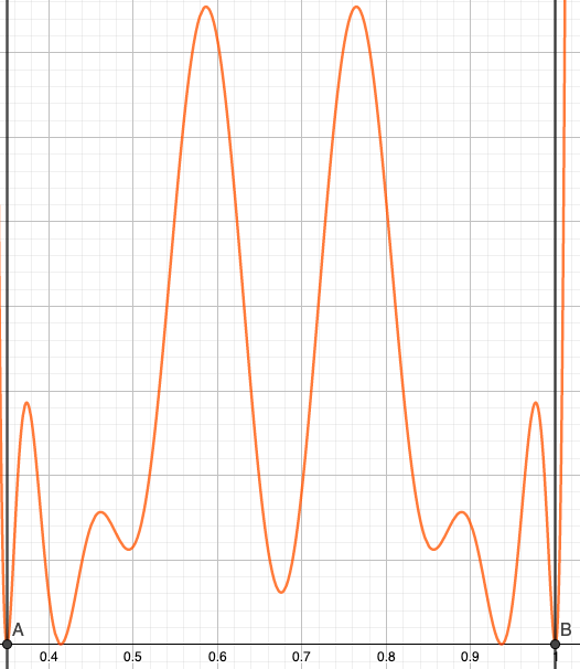
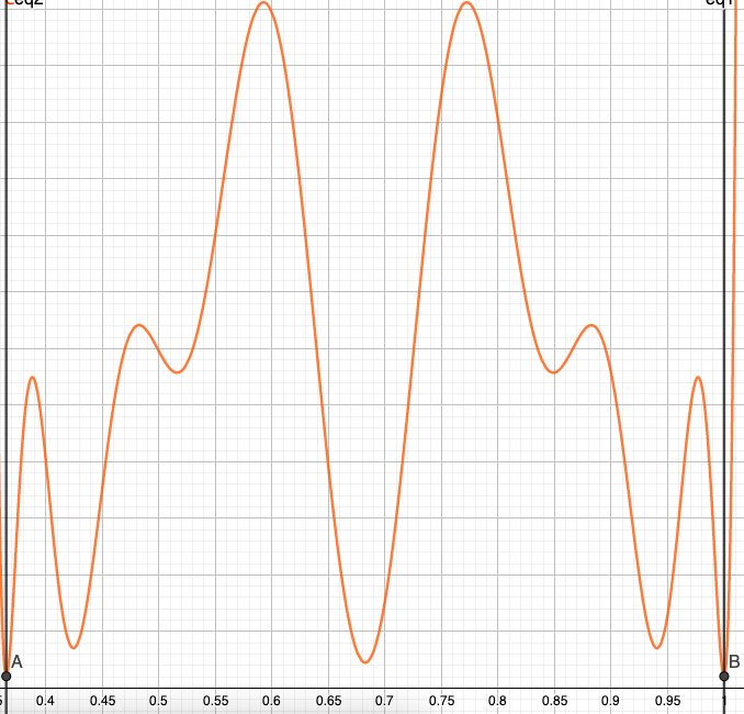
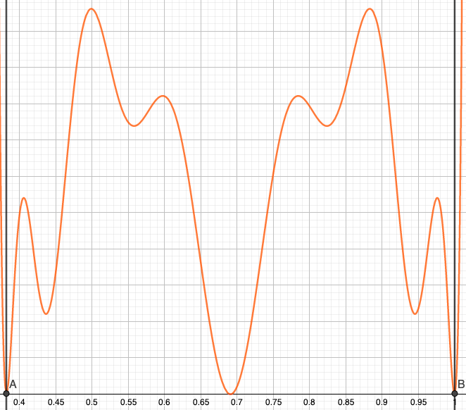
Figure 14. $G_{\kappa=8}^{E}(x)$, $x\in[E-1,1]$. Top : $\rho_{24}=-0.05$, bottom : $\rho_{24}=-0.36$. From left to right: $E=\mathcal{H}_{1}$, $E=1.365$, $E=\mathcal{H}_{0}$. $G_{\kappa=8}^{E}(x)>0$ in middle picture, but not in the other two.

19. The case of $\kappa=2$ in dimension 3

We illustrate the situation for $\kappa=2$, and the $4^{th}$ band, namely $(1+\mathcal{E}_{4},1+\mathcal{E}_{3})=(4/3,7/5)$. We use the linear combination $\sum_{j}\rho_{j\kappa}A_{j\kappa}$ where the coefficients $\rho_{j\kappa}$ are the same as in dimension 2, i.e. the ones found in Subsection 13.5.

Figure 15 shows the function $G_{\kappa=2}^{E}(x,y)$ at $E=1+\mathcal{E}_{4}=4/3$ and certain values of $y$. We observe a curious phenomenon. While the pattern observed is the same as the one occurring in dimension 2, the novelty is that it is now occurring simultaneously all for the same energy. In other words the pattern observed in dimension 3 for the $n^{th}$ band is the collection of the patterns observed for bands $1,2,...n$ in dimension 2. The graph of $G_{\kappa=2}^{E}(x,y)$ at $y=-2/3$ is not plotted because it is basically non-existant ($x=z=1$ is forced and so the graph is only defined at $x=1$, and $G_{\kappa=2}^{E=4/3}(1,-2/3)=0$). For $y\in[E-2,1]\setminus\{-2/3,-1/3,0,1/3,2/3,1\}$ $G_{\kappa=2}^{E}(x,y)$ appears to be strictly positive but that is irrelevant.

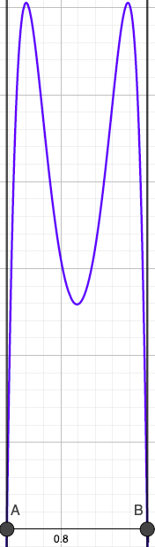
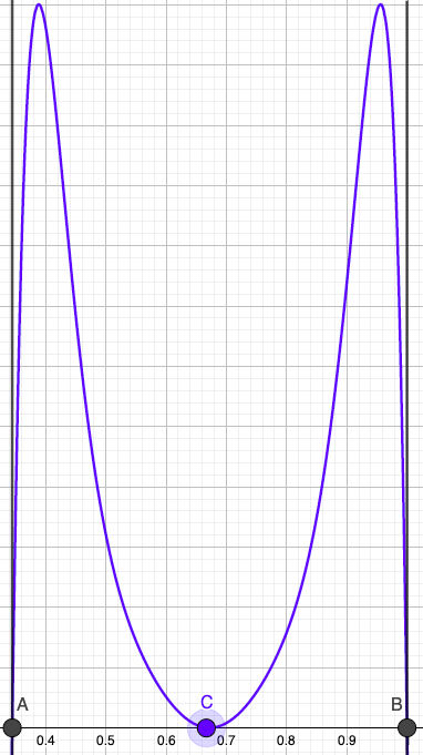
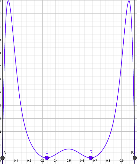
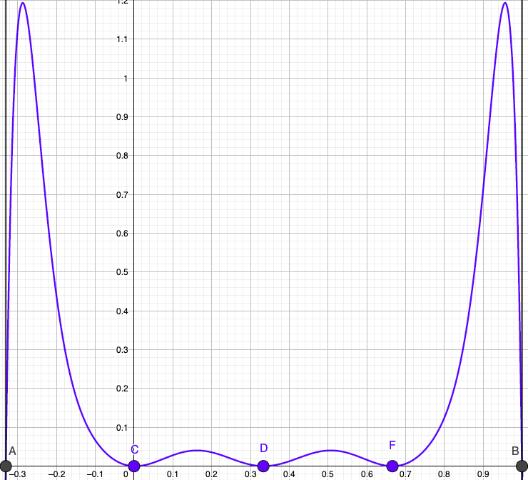
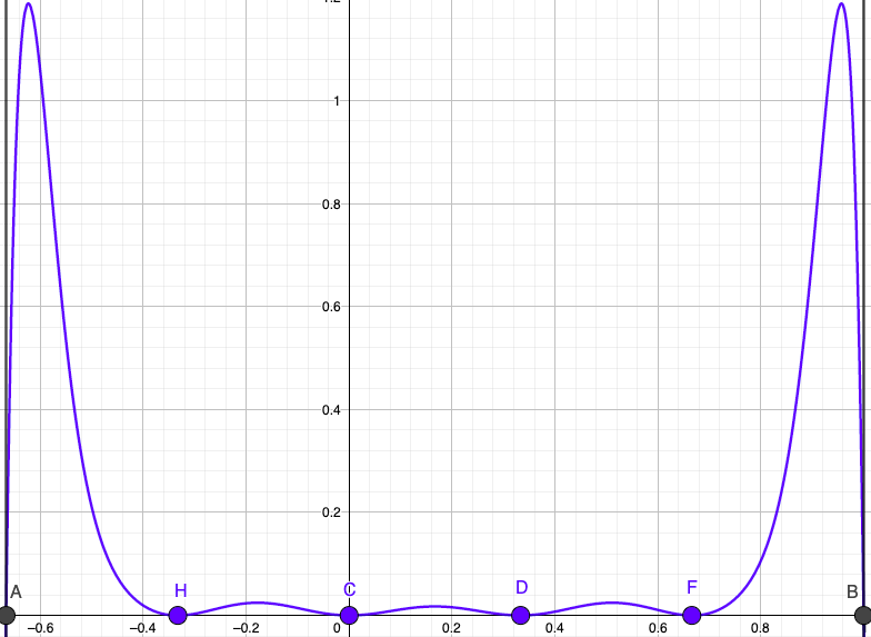
Figure 15. $G_{\kappa=2}^{E}(x,y)$. $E=1+\mathcal{E}_{4}=4/3$, $x\in[E-y-1,1]$. From left to right: $y=-1/3,0,1/3,2/3,1$.

Figure 16 shows the function $G_{\kappa=2}^{E}(x,y)$ at $E=1+\mathcal{E}_{3}=7/5$ and certain values of $y$.

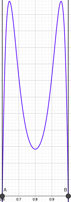
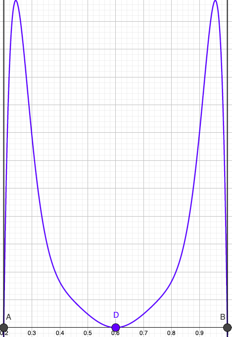
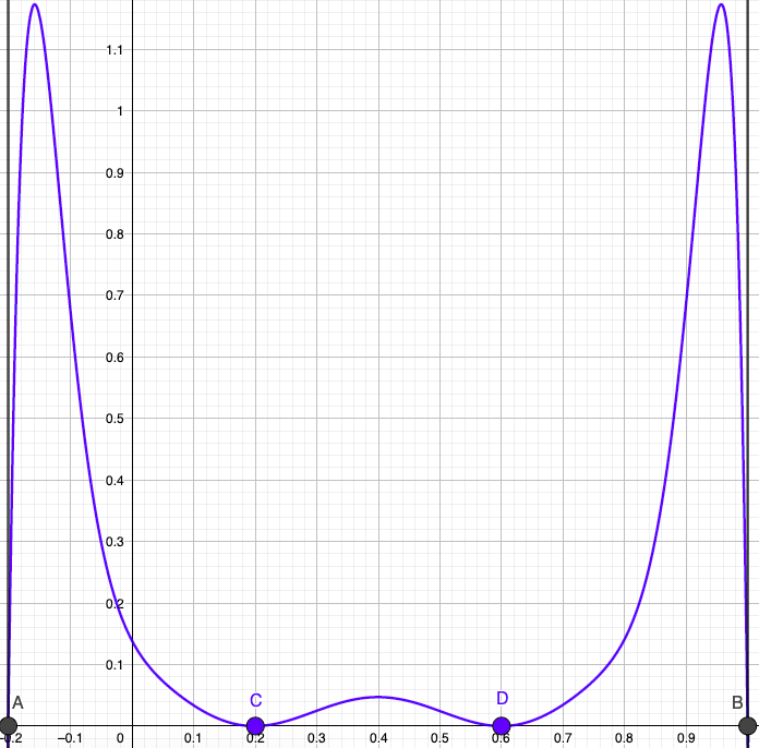
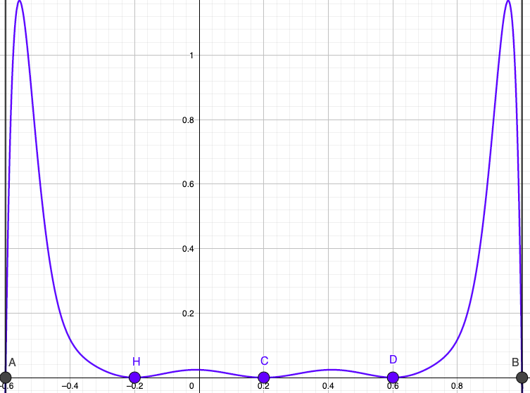
Figure 16. $G_{\kappa=2}^{E}(x,y)$. $E=1+\mathcal{E}_{3}=7/5$, $x\in[E-y-1,1]$. From left to right: $y=-1/5,1/5,3/5,1$.

20. A threshold in dimension 3 : An example to support Conjecture 1.18

We find a threshold for $\kappa=3$ in dimension 3. The example justifies our Conjecture 1.18 :

Example 20.1.

First we prove $E=\frac{3}{2\sqrt{7}}\in\bm{\Theta}_{1,\kappa=3}(\Delta[d=3])$. Note $\frac{3}{2\sqrt{7}}\simeq 0.56695$. To do this we follow the procedure in section 4.2, adpated to $d=3$. $E\in\bm{\Theta}_{1,\kappa}(\Delta[d=3])$ iff $\exists E\in[0,3]$, $Y_{i}\in[\max(E-2,-1),\min(E+2,1)]$, and $X_{i}\in[\max(E-Y_{i}-1,-1),\min(E-Y_{i}+1,1)]$, $i=0,1$, and $\omega_{0}<0$ such that

(20.1) $$\omega_{0}=\frac{g_{j\kappa}^{E}(X_{0},Y_{0})}{g_{j\kappa}^{E}(X_{1},Y_{1})}=\frac{g_{l\kappa}^{E}(X_{0},Y_{0})}{g_{l\kappa}^{E}(X_{1},Y_{1})},\quad\forall j,l\in\mathbb{N}^{*}.$$

Note $g_{j\kappa}^{E}(\cdot,\cdot)$ is given by (3.6). Thus we want to solve $[g_{j\kappa}^{E}(X_{0},Y_{0}),g_{l\kappa}^{E}(X_{1},Y_{1})]=0$. We make the simplifying assumption that $X_{0}=Y_{0}=E/3\neq\pm 1$. Thus, the latter commutator equation reduces to :

(20.2) $$m(X_{1})[U_{j\kappa-1}(E/3),U_{l\kappa-1}(X_{1})]+m(Y_{1})[U_{j\kappa-1}(E/3),U_{l\kappa-1}(Y_{1})]$$

$$\quad+m(E-X_{1}-Y_{1})[U_{j\kappa-1}(E/3),U_{l\kappa-1}(E-X_{1}-Y_{1})]=0.$$

By virtue of Corollary 2.4, this equation is satisfied if we further assume :

$$T_{\kappa=3}(E/3)=T_{\kappa=3}(X_{1})=T_{\kappa=3}(Y_{1})=T_{\kappa=3}(E-X_{1}-Y_{1}).$$

This is 3 equations, 3 unknowns ($E,X_{1},Y_{1}$). According to Python, a solution is $E=\frac{3}{2\sqrt{7}}$, $X_{1}=Y_{1}=2/\sqrt{7}$. We then check numerically that $\omega_{0}$ given by (20.1) is $<0$, and it is because $\omega_{0}=-1.8$. We therefore have $E\in\bm{\Theta}_{1,\kappa=3}(\Delta[d=3])$.

From our discussion in section 4.2, and notably the results in Table 2, we are inclined to believe that $\frac{3}{2\sqrt{7}}-\{\cos(l\pi/\kappa):0\leq l\leq\kappa\}\not\in\bm{\Theta}_{1,\kappa=3}(\Delta[d=2])$. Of course, our example is not a hard proof because we don’t know exactly what all the energies in $\bm{\Theta}_{1,\kappa=3}(\Delta[d=2])$ are. In any case, we also conjecture that $\frac{3}{2\sqrt{7}}-\{\cos(l\pi/\kappa):0\leq l\leq\kappa\}\not\in\bm{\Theta}_{\kappa=3}(\Delta[d=2])$.

21. Appendix : Recap of prior results ([GM2])

Table 7 are the bands $\subset\bm{\mu}_{\kappa}(\Delta)$ identified in [GM2]. These were obtained using the linear combination of conjugate operators (1.6) with $\rho_{j\kappa}=1$ if $j=1$, 0 otherwise.

$\kappa$	Intervals $\subset\bm{\mu}_{\kappa}(\Delta)$. $d=2$.	Intervals $\subset\bm{\mu}_{\kappa}(\Delta)$. $d=3$.
$1$	$(0,2)$	$[0,1)\cup(1,3)$
$2$	$(1,2)$	$(2,3)$
$3$	$(0.542477,1.000000)\cup(1.500000,2)$	$(2.5,3)$
$4$	$(1.026054,1.414214)\cup(1.707107,2)$	$(2.072,2.121)\cup(2.707,3)$
$5$	$(1.326098,1.618034)\cup(1.809017,2)$	$(2.353,2.427)\cup(2.809,3)$
$6$	$(1.511990,1.732051)\cup(1.866026,2)$	$(2.529,2.598)\cup(2.866,3)$
$7$	$(1.222521,1.246980)\cup(1.632351,1.801938)\cup(1.900969,2)$	$(2.645,2.703)\cup(2.901,3)$
$8$	$(1.382684,1.414214)\cup(1.713916,1.847760)\cup(1.923880,2)$	$(2.724,2.771)\cup(2.924,3)$

Table 7. Sets $\subset\bm{\mu}_{\kappa}(\Delta)\cap[0,d]$ found using the trivial linear combination ([GM2])

In [GM2] we conjectured exact formulas for the most of the band endpoints. In dimension 2 :

$$\begin{cases}\text{Interval}\ =\left(\ \_\_\ ,2\cos(\pi/\kappa)\right)\cup\left(1+\cos(\pi/\kappa),2\right),&\kappa=3-6,\\ \text{Interval}\ =\left(1+\cos(3\pi/\kappa),2\cos(2\pi/\kappa)\right)\cup\left(\ \_\_\ ,2\cos(\pi/\kappa)\right)\cup\left(1+\cos(\pi/\kappa),2\right),&\kappa=7,8.\end{cases}$$

And in dimension 3 :

$$\text{Interval}\ =\left(\ \_\_\ ,3\cos(\pi/\kappa)\right)\cup\left(2+\cos(\pi/\kappa),3\right),\quad\kappa=4-8.$$

22. Appendix : Algorithm details

The following simple algorithms were used to visually assess the positivity of $G_{\kappa}^{E}$.

When $\Delta$ in dimension $2$, we used the simple algorithm :

• For all $E\in[-2,2]$ :

  • let $y=E-x$

  • check if the function $x\mapsto G_{\kappa}^{E}(x)$ has same sign on the interval $x\in[\max(E-1,-1),\min(E+1,1)]$.

When $\Delta$ in dimension $3$, we used the simple algorithm :

• For all $E\in[0,3]$ :

• For all $y\in[\max(E-2,-1),\min(E+2,1)]$ :

  • let $z=E-x-y$

  • check if the function $x\mapsto G_{\kappa}^{E}(x,y)$ has same sign on the interval $x\in[\max(E-y-1,-1),\min(E-y+1,1)]$.

23. Appendix : The conjugate operator as a Fourier sine series

Let $A_{j\kappa}$ be given in (1.6), $\mathcal{F}=$ (3.1). $\mathcal{F}A_{j\kappa}\mathcal{F}^{-1}=(2\mathrm{i})^{-1}\sum_{i=1}^{d}[\sin(j\kappa\xi_{i})\frac{\partial}{\partial\xi_{i}}+\frac{\partial}{\partial\xi_{i}}\sin(j\kappa\xi_{i})]$. Let $f:[-\pi,\pi]\to\mathbb{R}$ be a $C^{1}$ function. Let $f=f_{+}+f_{-}$ be the decomposition of $f$ into an even $f_{+}$ and odd $f_{-}$ function. Consider conjugate operators of the form

(23.1) $$\mathbf{a}:=\frac{\mathrm{i}}{2}\sum_{i=1}^{d}f(\xi_{i})\frac{\partial}{\partial\xi_{i}}+\frac{\partial}{\partial\xi_{i}}f(\xi_{i}),\quad\mathbf{a}_{\pm}:=\frac{\mathrm{i}}{2}\sum_{i=1}^{d}f_{\pm}(\xi_{i})\frac{\partial}{\partial\xi_{i}}+\frac{\partial}{\partial\xi_{i}}f_{\pm}(\xi_{i}).$$

One has

$$\mathcal{F}[\Delta,\mathrm{i}\mathbf{a}]_{\circ}\mathcal{F}^{-1}=\sum_{i=1}^{d}\sin(\xi_{i})f(\xi_{i}),\quad\mathcal{F}[\Delta,\mathrm{i}\mathbf{a}_{\pm}]_{\circ}\mathcal{F}^{-1}=\sum_{i=1}^{d}\sin(\xi_{i})f_{\pm}(\xi_{i}).$$

Lemma 23.1.

If there is a continuous function $f$ such that the strict Mourre estimate (1.4) holds for $\Delta$ wrt. $\mathbf{a}$ in a neighborhood of $E$ then it holds for $\Delta$ wrt. $\mathbf{a}_{-}$ in a neighborhood of $E$.

Proof. Note that $(\xi_{1},...,\xi_{d})\in S_{E}\Leftrightarrow(-\xi_{1},...,-\xi_{d})\in S_{E}$. If the strict Mourre estimate holds for $\Delta$ wrt. $\mathbf{a}$ in a neighborhood of $E$, then $\exists t>0$ such that

(23.2) $$\chi_{\{E\}}\left(\sum_{i}\cos(\xi_{i})\right)\sum_{i=1}^{d}\sin(\xi_{i})(f_{+}(\xi_{i})+f_{-}(\xi_{i})) \geq t\cdot\chi_{\{E\}}\left(\sum_{i}\cos(\xi_{i})\right),\quad and$$

$$\chi_{\{E\}}\left(\sum_{i}\cos(-\xi_{i})\right)\sum_{i=1}^{d}\sin(-\xi_{i})(f_{+}(-\xi_{i})+f_{-}(-\xi_{i})) \geq t\cdot\chi_{\{E\}}\left(\sum_{i}\cos(-\xi_{i})\right).$$

Adding the 2 inequalities gives $\chi_{\{E\}}\left(\sum\cos(\xi_{i})\right)\sum_{i=1}^{d}\sin(\xi_{i})f_{-}(\xi_{i})\geq t\chi_{\{E\}}\left(\sum\cos(\xi_{i})\right)$, which means that the strict Mourre estimate holds for $\Delta$ wrt. $\mathbf{a}_{-}$ in a neighborhood of $E$. ∎ This Lemma means that if we assume a conjugate operator of the form (23.1), it is enough to restrict our attention to odd functions. Furthermore, odd $C^{1}$ functions can be expressed via a Fourier sine series. Thus a conjugate operator of the form (1.6) is in line with this observation, but also takes into account the $\kappa$–periodic specificity of the potential $V$.

24. $\kappa=10$ : thresholds in 1-1 correspondence with the nodes of a binary tree

Figure 17 illustrates a sequence of thresholds $\searrow 0$. To construct this sequence, the first point we place is $(0,T_{\kappa}(0))=(0,-1)$. Then we place pairs of points satisfying first the symmetry condition and then the level condition 2.3. Finally the last point is placed such that it satisfies the symmetry condition wrt. the last point constructed, as well as equals $(\cos(2\pi/\kappa),T_{\kappa}(\cos(2\pi/\kappa)))=(\cos(2\pi/\kappa),1)$ or $(\cos(4\pi/\kappa),T_{\kappa}(\cos(4\pi/\kappa)))=(\cos(4\pi/\kappa),1)$. This sequence is in 1-to-1 correspondence with the nodes of an infinite binary tree, because at every time we want to fulfill the level condition 2.3, i.e.  place $(X_{r},T_{\kappa}(X_{r}))$ such that $T_{\kappa}(X_{r})=T_{\kappa}(X_{q})$ and $T^{\prime}_{\kappa}(X_{r})\cdot T^{\prime}_{\kappa}(X_{q})<0$, we give ourselves the option of choosing from 2 different branches of $T_{\kappa}(\cdot)$ (we could choose many more branches !).

Figure 17. $T_{\kappa=10}(x)$. A sequence of threshold solutions $\searrow 0$.

References

- [ABG] W.O. Amrein, A. Boutet de Monvel, and V. Georgescu: -groups, commutator methods and spectral theory of -body hamiltonians, Birkhäuser, (1996).
- [BSa] A. Boutet de Monvel, J. Sahbani: On the spectral properties of discrete Schrödinger operators: the multi-dimensional case, Rev. in Math. Phys. 11, No. 9, p. 1061–1078, (1999).
- [FH] R. Froese, I. Herbst: Exponential bounds and absence of positive eigenvalues for N-body Schrödinger operators., Comm. Math. Phys. 87, no. 3, p. 429–447, (1982/83).
- [GM1] S. Golénia, M. Mandich : Limiting absorption principle for discrete Schrödinger operators with a Wigner-von Neumann potential and a slowly decaying potential, Ann. Henri Poincaré 22, 83–120, (2021).
- [GM2] S. Golénia, M. Mandich : Bands of absolutely continuous spectrum for lattice Schrödinger operators with a more general long range condition, J. Math. Phys., Vol. 62, Issue 9, (2021).
- [GM4] S. Golénia, M. Mandich : Additional numerical and graphical evidence to support some Conjectures on discrete Schrödinger operators with a more general long range condition, preprint on arxiv (not intended for publication).
- [IJ] K. Ito, A. Jensen : Branching form of the resolvent at thresholds for multi-dimensional discrete Laplacians, J. Funct. Anal., 277, No. 4, 965–993, (2019).
- [Ki] A. Kiselev: Imbedded singular continuous spectrum for Schrödinger operators, J. of the AMS, Vol. 18, Num. 3, (2005), 571–603.
- [Li1] W. Liu : Absence of singular continuous spectrum for perturbed discrete Schrödinger operators, J. of Math. Anal. and Appl., Vol. 472, Issue 2, 1420–1429, (2019).
- [Li2] W. Liu : Criteria for embedded eigenvalues for discrete Schrödinger Operators, International Mathematics Research Notices, rnz262, https://doi.org/10.1093/imrn/rnz262, (2019).
- [Mo1] E. Mourre: Absence of singular continuous spectrum for certain self-adjoint operators, Comm. Math. Phys., 78, p. 391–408, (1981).
- [Mo2] E. Mourre: Opérateurs conjugués et propriétés de propagation, Comm. Math. Phys., 91, p. 279–300, (1983).
- [Ma] M. Mandich : Sub-exponential decay of eigenfunctions for some discrete Schrödinger operators, J. Spectr. Theory 9, 21–77, (2019).
- [NoTa] Y. Nomura, K. Taira : Some properties of threshold eigenstates and resonant states of discrete Schrödinger operators, Ann. Henri Poincaré 21, 2009–2030, (2020).