Small-Signal Stability Analysis of Numerical Integration Methods

Abstract

The paper provides a novel framework to study the accuracy and stability of numerical integration schemes when employed for the time domain simulation of power systems. A matrix pencil-based approach is adopted to evaluate the error between the dynamic modes of the power system and the modes of the approximated discrete-time system arising from the application of the numerical method. The proposed approach can provide meaningful insights on how different methods compare to each other when applied to a power system, while being general enough to be systematically utilized for, in principle, any numerical method. The framework is illustrated for a handful of well-known explicit and implicit methods, while simulation results are presented based on the WSCC $9$-bus system, as well as on a $1,479$-bus dynamic model of the All-Island Irish Transmission System.

I Introduction

I-A Motivation

Time domain simulations are an essential component of power system dynamic analysis and security assessment. In general, a time domain simulation consists in integrating the dynamic power system model for a set of initial conditions and through a proper numerical method. The need for the application of a numerical method leads to an approximated representation of the original system’s behavior, with the deviation between exact and obtained solution being dependent upon the method’s properties and parameters, as well as on the structure of the modeled dynamics. The goal of this work is to provide a novel and systematic approach to study the approximation induced to the dynamic modes of power systems by numerical Time Domain Integration (TDI) methods.

I-B Literature Review

A dynamic power system model is conventionally described by a set of non-linear and stiff Differential Algebraic Equations (DAEs) [1]. The TDI of a power system often relies on the implementation of an implicit numerical method, since explicit schemes – such as the Forward Euler Method (FEM) – perform poorly for stiff problems. The implicit method most commonly utilized in power system dynamic simulations is arguably the Implicit Trapezoidal Method (ITM), yet a number of schemes have been proposed to achieve the best compromise between accuracy and efficiency of simulation, see [2, 1, 3, 4, 5, 6, 7, 8]. For example, some studies propose to combine or substitute the ITM with a hyperstable scheme, such as the Backward Euler Method (BEM), with a scope to improve the handling of discontinuities and avoid undamped numerical oscillations under large time steps [3, 7].

The precision of a TDI is typically assessed on the basis of certain metrics, such as the local and global truncation errors of the numerical scheme employed. Truncation errors provide a good measure of the deviation between exact and numerically computed trajectories and are the standard criterion used for the implementation of automatic step size and order control techniques [4, 5]. However, the ability of a TDI method to prevent the exponential growth of truncation errors cannot be predicted with the truncation errors. Information on the latter is given instead from the characterization of TDI methods according to their properties of numerical stability. As a matter of fact, the major advantage of implicit over explicit methods is that they outperform in terms of numerical stability. For example, the ITM is symmetrically A-stable, i.e. it converges for stable and diverges for unstable trajectories, whereas the FEM is unstable, i.e. it always diverges for sufficiently large time steps.

The classical approach to stability characterization of a TDI method is to check its response when applied to a linear test equation. Consequently, the main limitation of this approach is that it is only qualitative, since it does not involve the dynamics of the specific model to be integrated, and it is thus not suitable for accuracy assessment. On the contrary, this work is concerned with the problem of providing a unified framework, based on Small-Signal Stability Analysis (SSSA), to study the accuracy and stability of numerical methods applied for the TDI of power systems. This problem is tackled by introducing a generic model of numerical method that admits as special cases the most important families of methods, the behavior of which is then analyzed by studying the associated matrix pencils [9]. The proposed formulation allows quantifying the spurious distortion that a TDI method introduces to the dynamic modes of the power system model to which it is applied, as well as systematically realizing relevant analysis tools already available in the literature. In this vein we cite [10], which presents a tool to assess the numerical approximation of the motion of simple linear networks by means of distortion maps.

I-C Contributions

The specific contributions of the paper are as follows.

• A general numerical stability analysis framework based on matrix pencils that, in principle, is applicable to any numerical TDI scheme.

• The proposed framework is utilized to evaluate the numerical distortion introduced by TDI methods to the dynamic modes of power system models.

• For certain Runge-Kutta (RK) methods, it is also shown that the pencil to be studied emerges as an extension of the method’s growth function.

• A discussion on how the proposed approach can be employed to estimate useful upper time step bounds that satisfy certain accuracy criteria, as well as to provide fair computational-burden comparisons of different methods.

It is important to note that one cannot “compare” the proposed framework to a specific integration method. Rather, one can use the proposed approach to define the numerical stability properties of such an integration method.

I-D Organization

The remainder of the paper is organized as follows. Section II describes the dynamic power system model and provides preliminaries on the numerical TDI. The proposed framework to study the stability and accuracy of power system TDI is presented in Section III. The case studies are discussed in Section IV based on the well-known WSCC system and a dynamic model of the All-Island Irish Transmission System (AIITS). Finally, conclusions are drawn in Section V.

II Integration of Power System Model

II-A Power System Model

The mathematical model that describes the dynamics of a power system can be formulated as follows:

$$\boldsymbol{\rm E}\,{\mbox{$\boldsymbol{\rm x}$}}^{\prime}(t) =\boldsymbol{\phi}(\mbox{$\boldsymbol{\rm x}$}(t))\,,$$ (1)

where $\boldsymbol{\rm E}\in\mathbb{R}^{r\times r}$; $\mbox{$\boldsymbol{\rm x}$}:[0,\infty)\rightarrow\mathbb{R}^{r}$ is the column vector of the system’s variables and ${\mbox{$\boldsymbol{\rm x}$}}^{\prime}$ denotes the time derivative of $\boldsymbol{\rm x}$; $\boldsymbol{\rm\phi}:\mathbb{R}^{r}\rightarrow\mathbb{R}^{r}$ is a set of non-linear functions that defines the equations of the system. Discrete variables in (1) are modeled implicitly, i.e., each discontinuous change in the system leads to a jump from (1) to a new continuous set of equations in the same form. A relevant special case is when (1) is formulated as a set of explicit Differential Algebraic Equations, i.e.:

$$\boldsymbol{\rm E}=\begin{bmatrix}\boldsymbol{I}_{m_{x}}&\boldsymbol{0}_{m_{x},m_{y}}\\ \boldsymbol{0}_{m_{y},m_{x}}&\boldsymbol{0}_{m_{y},m_{y}}\\ \end{bmatrix},\,\boldsymbol{\phi}(\mbox{$\boldsymbol{\rm x}$}(t))=\begin{bmatrix}\boldsymbol{f}(\boldsymbol{x}(t),\boldsymbol{y}(t))\\ \boldsymbol{g}(\boldsymbol{x}(t),\boldsymbol{y}(t))\\ \end{bmatrix}\,,$$ (2)

and $\mbox{$\boldsymbol{\rm x}$}(t)=[\boldsymbol{x}^{\scriptscriptstyle\rm T}(t)\ \boldsymbol{y}^{\scriptscriptstyle\rm T}(t)]^{\scriptscriptstyle\rm T}$, where $\boldsymbol{x}:[0,\infty)\rightarrow\mathbb{R}^{m_{x}}$ and $\boldsymbol{y}:[0,\infty)\rightarrow\mathbb{R}^{m_{y}}$ are the state and algebraic variables; and $\boldsymbol{f}:\mathbb{R}^{m_{x}+m_{y}}\rightarrow\mathbb{R}^{m_{x}}$, $\boldsymbol{g}:\mathbb{R}^{m_{x}+m_{y}}\rightarrow\mathbb{R}^{m_{y}}$, are non-linear functions that define the differential and algebraic equations, respectively; $\boldsymbol{I}_{m_{x}}$ denotes the $m_{x}\times m_{x}$ identity matrix and $\boldsymbol{0}_{m_{x},m_{y}}$ the $m_{x}\times m_{y}$ zero matrix. Equivalently, one has:

$${\boldsymbol{x}}^{\prime}(t) =\boldsymbol{f}(\boldsymbol{x}(t),\boldsymbol{y}(t))\,,$$ (3)

$$\boldsymbol{0}_{m_{y},1} =\boldsymbol{g}(\boldsymbol{x}(t),\boldsymbol{y}(t))\,.$$

Formulation (3) is the standard model employed in the literature for transient and voltage stability studies [11]. Yet, the main results of this work hold also for the more general model (1) and, thus, (1) is the starting point considered in this paper.

II-B Numerical Integration

A TDI method for power systems is a discrete-time approximation employed to solve system (1) for a defined time period and set of initial conditions. We propose the following generic model to describe a TDI method.

Definition 1.

In an implicit form, a TDI method applied to system (1) can be described by a discrete-time system, as follows:

$$\boldsymbol{0}_{r,1}=\boldsymbol{\eta}(\mbox{$\boldsymbol{\rm x}$}_{t},\mbox{$\boldsymbol{\rm x}$}_{t-h},\mbox{$\boldsymbol{\rm x}$}_{t-a_{1}h},\mbox{$\boldsymbol{\rm x}$}_{t-a_{2}h},\ldots,\mbox{$\boldsymbol{\rm x}$}_{t-a_{\rho}h})\,,$$ (4)

where $h$ is the integration time step size, which can be constant or varying; $r=m_{x}+m_{y}$; $\boldsymbol{\eta}:\mathbb{R}^{(\rho+2)r}\rightarrow\mathbb{R}^{r}$ is a vector of non-linear functions; $\mbox{$\boldsymbol{\rm x}$}_{t}:\mathbb{N}^{*}h\rightarrow\mathbb{R}^{r}$; and $a_{i}>0$, $a_{i}\neq 1$, $i=1,2,\ldots,\rho$.

The discrete-time system (4) covers most elements of the two largest and most important families of TDI methods, namely RK and linear multistep methods. We clarify here that (4) is expressed in an implicit form but this should not be confused with the method being implicit or not. In fact, both explicit and implicit methods can be represented in the form of (4). With this regard, we propose the following definition of explicit numerical methods applied to system (1).

Definition 2.

If, without resorting to further approximations, system (4) can be equivalently rewritten in the form:

$$\boldsymbol{\rm E}\,\mbox{$\boldsymbol{\rm x}$}_{t}=\boldsymbol{\theta}(\mbox{$\boldsymbol{\rm x}$}_{t-h},\mbox{$\boldsymbol{\rm x}$}_{t-a_{1}h},\mbox{$\boldsymbol{\rm x}$}_{t-a_{2}h},\ldots,\mbox{$\boldsymbol{\rm x}$}_{t-a_{\rho}h})\,,$$ (5)

where $\boldsymbol{\rm E}$ is given by (2); and $\boldsymbol{\theta}:\mathbb{R}^{(\rho+2)r}\rightarrow\mathbb{R}^{r}$; then it describes an explicit numerical method. Otherwise, the method is implicit.

Implicit methods involve an extra computation compared to explicit methods, i.e. they require the solution of system (4) for $\mbox{$\boldsymbol{\rm x}$}_{t}$. This computation is done iteratively at every step of the integration. For instance, the $i$-th iteration of Newton’s method when applied to (4) is:

$$\mbox{$\boldsymbol{\rm x}$}^{(i)}_{t}=\mbox{$\boldsymbol{\rm x}$}^{(i-1)}_{t}-\left[\frac{\partial\boldsymbol{\eta}^{(i-1)}}{\partial\mbox{$\boldsymbol{\rm x}$}^{(i-1)}_{t}}\right]^{-1}\boldsymbol{\eta}^{(i-1)}\,,$$ (6)

where ${\partial\boldsymbol{\eta}}/{\partial\mbox{$\boldsymbol{\rm x}$}_{t}}$ denotes the Jacobian matrix of (4). The fact that such computational step is not required by explicit methods is the reason why the latter are still the option preferred by some software tools. We cite, for example, the use of the explicit modified Euler method in [12]. Hence, for completeness, this paper discusses both explicit and implicit methods.

II-C Problem Stiffness and Small-Signal Model

The TDI of a power system constitutes a stiff problem, i.e., the time constants that define the differential equations of the model span multiple time scales. A measure of stiffness is given by the stiffness ratio of the corresponding small-signal model. Let $\mbox{$\boldsymbol{\rm x}$}_{o}$ be an equilibrium point of (1). Then, linearization around $\mbox{$\boldsymbol{\rm x}$}_{o}$ gives:

$$\boldsymbol{\rm E}\,\Delta\mbox{$\boldsymbol{\rm x}$}^{\prime}(t)=\boldsymbol{\rm A}\,\Delta\mbox{$\boldsymbol{\rm x}$}(t)\,,$$ (7)

where $\boldsymbol{\rm A}=\partial\boldsymbol{\phi}/\partial\mbox{$\boldsymbol{\rm x}$}$ and $\Delta\mbox{$\boldsymbol{\rm x}$}(t)=\mbox{$\boldsymbol{\rm x}$}-\mbox{$\boldsymbol{\rm x}$}_{o}$. The eigenvalues of (7) are the solutions of the characteristic equation:

$${\rm det}(s\boldsymbol{\rm E}-\boldsymbol{\rm A})=0\,,$$ (8)

where the family of matrices $s\boldsymbol{\rm E}-\boldsymbol{\rm A}$ parameterized by $s\in\mathbb{C}$ is called the matrix pencil of system (7) [9]. In total, the pencil $s\boldsymbol{\rm E}-\boldsymbol{\rm A}$ has $\upnu={\rm rank}(s\boldsymbol{\rm E}-\boldsymbol{\rm A})$ finite eigenvalues plus the infinite eigenvalue with multiplicity $r-\upnu$. Moreover, (7) is asymptotically stable if and only if the real parts of all finite eigenvalues $s^{*}$ of $s\boldsymbol{\rm E}-\boldsymbol{\rm A}$ satisfy ${\rm Re}(s^{*})<0$. In practice, the eigenvalues of $s\boldsymbol{\rm E}-\boldsymbol{\rm A}$ are computed numerically, see [13]. We finally provide the following definition.

Definition 3.

Assume that (7) is asymptotically stable and let $s_{i}=\alpha_{i}+\jmath\beta_{i}$, $i=1,2,\ldots,\upnu$, be the $i$-th finite eigenvalue of $s\boldsymbol{\rm E}-\boldsymbol{\rm A}$. Let also $\sigma_{\max}=\max\{|\alpha_{i}|\}$, $\sigma_{\min}=\min\{|\alpha_{i}|\}$ denote the maximum, minimum exponential decay rates of the system, respectively. Then, the stiffness ratio of (7) is [14]:

$$\mathcal{S}=\frac{\sigma_{\max}}{\sigma_{\min}}\,.$$ (9)

It is relevant to note that the definition of stiffness is not unique. For example, an alternative definition may also take into account the effect of the imaginary parts $\beta_{i}$, e.g. by defining as measure of stiffness the ratio of the finite eigenvalues with largest and smallest magnitude.

Apart from its presence in (9), the maximum exponential decay rate $\sigma_{\max}$ is an index commonly employed by software tools to make an heuristic estimation of the maximum admissible integration time step based on empirical rules, to prevent either that the fastest dynamics of the system are filtered out, or, in the case of an explicit method, that convergence is compromised [16]. On the contrary, in this paper we systematically evaluate the error of the TDI method in approximating the dynamic modes of the system which allows extracting upper time step bounds with higher accuracy.

II-D Classical Stability Analysis

This section briefly recalls the classical approach to stability analysis of numerical TDI methods. The stability of a numerical method for ordinary differential equations is traditionally tested and classified by applying the method to Dahlquist’s test equation:

$$\xi^{\prime}(t)=\lambda\;\xi(t)\,,$$ (10)

where $\lambda\in\mathbb{C}$. Let apply an integration method to (10) so that:

$$\xi_{t}=\mathcal{R}(\lambda h)\;\xi_{t-h}\,,$$ (11)

where $\mathcal{R}(\lambda h)$ is the method’s growth or stability function. Then, the stability region of the method is defined by the set:

$$\{\lambda\in\mathbb{C}\,:\ |\mathcal{R}(\lambda h)|<1\}\,.$$ (12)

As an example, consider the application of the ITM to (10):

$$\xi_{t}=\xi_{t-h}+0.5h\lambda\xi_{t-h}+0.5h\lambda\xi_{t}\,,$$ (13)

which can be equivalently written in the form of (11), where:

$$\mathcal{R}(\lambda h)=\frac{1+0.5\lambda h}{1-0.5\lambda h}\,.$$ (14)

From (12), (14), we have that the stability region of the ITM is the left half of the $S$-plane.

For RK methods, the growth function can be written as [17]:

$$\mathcal{R}(\lambda h)=\frac{{\rm det}(\boldsymbol{I}_{\rho}-\lambda h\boldsymbol{\rm Q}+\lambda h\boldsymbol{\rm e}_{\rho}\boldsymbol{\rm r})}{{\rm det}(\boldsymbol{I}_{\rho}-\lambda h\boldsymbol{\rm Q})}\,,$$ (15)

where $\rho$ is the method’s number of stages; $\boldsymbol{\rm e}_{\rho}$ is the $\rho\times 1$ vector of ones; and $[\boldsymbol{\rm Q}^{\scriptscriptstyle\rm T}\ \boldsymbol{\rm r}^{\scriptscriptstyle\rm T}]^{\scriptscriptstyle\rm T}$, is the method’s generating matrix, $\boldsymbol{\rm Q}\in\mathbb{R}^{\rho\times\rho}$, $\boldsymbol{\rm r}\in\mathbb{R}^{1\times\rho}$. Note that explicit RK methods have ${\rm det}(\boldsymbol{I}_{\rho}-h\lambda\boldsymbol{\rm Q})=1$, and thus their growth function is a polynomial of $\lambda h$. On the other hand, the growth function of an implicit RK method is a quotient of two polynomials of $\lambda h$.

III Matrix Pencil-based Numerical Analysis

III-A Proposed Approach

In this section we provide a general approach to study the numerical distortion caused by TDI methods to the dynamic modes of system (1). First, we prove that the approximation introduced by any numerical method applied to a system in the form of (1) can be studied through a linear matrix pencil. Consider the discrete-time system (4) and assume for simplicity but without loss of generality that $h$ is constant. Then, linearization of the system around the equilibrium $\mbox{$\boldsymbol{\rm x}$}_{o}$ of (1), which is also a fixed point of (4), gives:

$$\boldsymbol{0}_{r,1}= \frac{\partial\boldsymbol{\eta}}{\partial\mbox{$\boldsymbol{\rm x}$}_{t}}\Delta\mbox{$\boldsymbol{\rm x}$}_{t}+\frac{\partial\boldsymbol{\eta}}{\partial\mbox{$\boldsymbol{\rm x}$}_{t-h}}\Delta\mbox{$\boldsymbol{\rm x}$}_{t-h}+\frac{\partial\boldsymbol{\eta}}{\partial\mbox{$\boldsymbol{\rm x}$}_{t-a_{1}h}}\Delta\mbox{$\boldsymbol{\rm x}$}_{t-a_{1}h}$$

$$+\frac{\partial\boldsymbol{\eta}}{\partial\mbox{$\boldsymbol{\rm x}$}_{t-a_{2}h}}\Delta\mbox{$\boldsymbol{\rm x}$}_{t-a_{2}h}+\ldots+\frac{\partial\boldsymbol{\eta}}{\partial\mbox{$\boldsymbol{\rm x}$}_{t-a_{\rho}h}}\Delta\mbox{$\boldsymbol{\rm x}$}_{t-a_{\rho}h}\,.$$ (16)

We provide the following proposition.

Proposition 1.

The stability properties of system (16) can be assessed by studying the stability of a linear discrete-time system in the form:

$$\tilde{\boldsymbol{\rm E}}\,\mbox{$\boldsymbol{\rm y}$}_{t}=\tilde{\boldsymbol{\rm A}}\,\mbox{$\boldsymbol{\rm y}$}_{t-h}\,.$$ (17)

The proof of Proposition 1 is provided in the Appendix. Then, the stability of (17) can be seen through the eigenvalues of the matrix pencil $\tilde{z}\tilde{\boldsymbol{\rm E}}-\tilde{\boldsymbol{\rm A}}$. In particular, (17) is asymptotically stable if and only if all finite eigenvalues $\tilde{z}^{*}$ of its pencil $\tilde{z}\tilde{\boldsymbol{\rm E}}-\tilde{\boldsymbol{\rm A}}$ lie within the open unit disc, or equivalently, $|\tilde{z}^{*}|<1$.

The eigenvalues of $\tilde{z}\,\tilde{\boldsymbol{\rm E}}-\tilde{\boldsymbol{\rm A}}$ represent, in the $Z$-plane, the small-disturbance dynamic modes of (1) as approximated by the numerical method (4). Let $\tilde{z}_{k}$ be an eigenvalue of $\tilde{z}\,\tilde{\boldsymbol{\rm E}}-\tilde{\boldsymbol{\rm A}}$ approximating the $k$-th dynamic mode of the power system model, which is represented by the finite eigenvalue $s_{k}=\alpha+\jmath\beta$ of $s\boldsymbol{\rm E}-\boldsymbol{\rm A}$. Then, the two eigenvalues become directly comparable by mapping the one to the domain of the other. Mapping $\tilde{z}_{k}$ from the $Z$-plane to the $S$-plane, we get:

$$\tilde{s}_{k}=\frac{1}{h}{\rm log}(\tilde{z}_{k})=\tilde{\alpha}+\jmath\tilde{\beta}\,,$$ (18)

where ${\rm log}(\cdot)$ denotes the complex logarithm. Then, the numerical distortion caused to the $k$-th mode by the TDI method is:

$${d}_{s,k}=\tilde{s}_{k}-s_{k}\,.$$ (19)

The distortion caused to the damping of the $k$-th mode is:

$${d}_{\zeta,k}=\tilde{\zeta}_{k}-\zeta_{k}\,,$$ (20)

where $\zeta_{k}=-{\alpha}/({\alpha^{2}+\beta^{2}})$. Positive (negative) values of ${d}_{\zeta,k}$ indicate that the mode is overdamped (underdamped).

III-B Illustrative Examples

This section discusses the matrix pencils that characterize the stability and accuracy of some well-known integration TDI methods. In particular, six methods are considered, namely (i) FEM, (ii) Runge-Kutta 4 (RK4), (iii) BEM, (iv) ITM, (v) 2-Stage Diagonally Implicit Runge-Kutta (2S-DIRK) and (vi) 2-step Backward Differentiation Formula (BDF2). These methods are also employed for the case studies of Section IV.

Forward Euler Method (FEM)

The FEM is the simplest among all integration schemes. When applied to system (1), the FEM reads:

$$\boldsymbol{\rm E}\mbox{$\boldsymbol{\rm x}$}_{t}=\boldsymbol{\rm E}\mbox{$\boldsymbol{\rm x}$}_{t-h}+h\boldsymbol{\phi}(\mbox{$\boldsymbol{\rm x}$}_{t-h})\,,$$ (21)

where $\mbox{$\boldsymbol{\rm x}$}^{\prime}(t)$ is approximated with the finite difference formula $(\mbox{$\boldsymbol{\rm x}$}_{t}-\mbox{$\boldsymbol{\rm x}$}_{t-h})/h$. Linearization of (21) around $\mbox{$\boldsymbol{\rm x}$}_{o}$ gives:

$$\boldsymbol{\rm E}\Delta\mbox{$\boldsymbol{\rm x}$}_{t}=\boldsymbol{\rm E}\Delta\mbox{$\boldsymbol{\rm x}$}_{t-h}+h\boldsymbol{\rm A}\Delta\mbox{$\boldsymbol{\rm x}$}_{t-h}\,.$$ (22)

Equivalently, (22) can be rewritten as a discrete-time system in the form of (17) with pencil $\tilde{z}\tilde{\boldsymbol{\rm E}}-\tilde{\boldsymbol{\rm A}}$, where $\mbox{$\boldsymbol{\rm y}$}_{t}\equiv\Delta\mbox{$\boldsymbol{\rm x}$}_{t}$ and:

$$\tilde{\boldsymbol{\rm E}} ={\boldsymbol{\rm E}}\,,\quad\tilde{\boldsymbol{\rm A}}={\boldsymbol{\rm E}}+h{\boldsymbol{\rm A}}\,.$$ (23)

Runge-Kutta 4 (RK4)

The classical RK4 is a fourth-order method and is the most well-known explicit RK method. Applied to (1), the RK4 method reads:

$$\boldsymbol{\rm E}\,\mbox{$\boldsymbol{\rm x}$}_{t} =\boldsymbol{\rm E}\,\mbox{$\boldsymbol{\rm x}$}_{t-h}+\frac{h}{6}(\boldsymbol{k}_{1}+2\boldsymbol{k}_{2}+2\boldsymbol{k}_{3}+\boldsymbol{k}_{4})\,,$$ (24)

$$\boldsymbol{k}_{1} =\boldsymbol{\phi}(\mbox{$\boldsymbol{\rm x}$}_{t-h})\,,\hskip 49.79231pt\boldsymbol{k}_{2}=\boldsymbol{\phi}(\mbox{$\boldsymbol{\rm x}$}_{t-h}+0.5h\boldsymbol{k}_{1})\,,$$

$$\boldsymbol{k}_{3} =\boldsymbol{\phi}(\mbox{$\boldsymbol{\rm x}$}_{t-h}+0.5h\boldsymbol{k}_{2})\,,\quad\boldsymbol{k}_{4}=\boldsymbol{\phi}(\mbox{$\boldsymbol{\rm x}$}_{t-h}+h\boldsymbol{k}_{3})\,.$$

Linearization of (24) yields the following expressions:

$$\boldsymbol{k}_{1} =\boldsymbol{\rm A}\Delta\mbox{$\boldsymbol{\rm x}$}_{t-h}\,,\hskip 56.9055pt\boldsymbol{k}_{2}=\boldsymbol{\rm A}(\Delta\mbox{$\boldsymbol{\rm x}$}_{t-h}+0.5h\boldsymbol{k}_{1})\,,$$ (25)

$$\boldsymbol{k}_{3} =\boldsymbol{\rm A}(\Delta\mbox{$\boldsymbol{\rm x}$}_{t-h}+0.5h\boldsymbol{k}_{2})\,,\quad\boldsymbol{k}_{4}=\boldsymbol{\rm A}(\Delta\mbox{$\boldsymbol{\rm x}$}_{t-h}+h\boldsymbol{k}_{3})\,.$$

Equivalently, the linearized method can be written in the form of (17) with matrix pencil $\tilde{z}\tilde{\boldsymbol{\rm E}}-\tilde{\boldsymbol{\rm A}}$, where $\mbox{$\boldsymbol{\rm y}$}_{t}\equiv\Delta\mbox{$\boldsymbol{\rm x}$}_{t}$ and:

$$\tilde{\boldsymbol{\rm E}} ={\boldsymbol{\rm E}}\,,$$ (26)

$$\tilde{\boldsymbol{\rm A}} ={\boldsymbol{\rm E}}+h{\boldsymbol{\rm A}}+\frac{(h{\boldsymbol{\rm A}})^{2}}{2}+\frac{(h{\boldsymbol{\rm A}})^{3}}{6}+\frac{(h{\boldsymbol{\rm A}})^{4}}{24}\,.$$

Backward Euler Method (BEM)

The BEM is the implicit variant of the FEM and is a hyperstable method with stability region the part of the $S$-plane that is outside the unit disk centered at 1. When applied to system (1), the BEM reads:

$$\boldsymbol{\rm E}\mbox{$\boldsymbol{\rm x}$}_{t}=\boldsymbol{\rm E}\mbox{$\boldsymbol{\rm x}$}_{t-h}+h\boldsymbol{\phi}(\mbox{$\boldsymbol{\rm x}$}_{t})\,.$$ (27)

Linearization of (27) leads to a discrete-time system in the form of (17), where $\mbox{$\boldsymbol{\rm y}$}_{t}\equiv\Delta\mbox{$\boldsymbol{\rm x}$}_{t}$ and:

$$\tilde{\boldsymbol{\rm E}} ={\boldsymbol{\rm E}}-h{\boldsymbol{\rm A}}\,,\quad\tilde{\boldsymbol{\rm A}}={\boldsymbol{\rm E}}\,.$$ (28)

Implicit Trapezoidal Method (ITM)

The ITM can be interpreted as the weighted sum of the FEM and BEM with equal weights for the two methods. Applied to system (1), the ITM reads:

$$\boldsymbol{\rm E}\mbox{$\boldsymbol{\rm x}$}_{t}=\boldsymbol{\rm E}\mbox{$\boldsymbol{\rm x}$}_{t-h}+0.5h\boldsymbol{\phi}(\mbox{$\boldsymbol{\rm x}$}_{t-h})+0.5h\boldsymbol{\phi}(\mbox{$\boldsymbol{\rm x}$}_{t})\,.$$ (29)

Linearization of (29) leads to a system in the form of (17), where $\mbox{$\boldsymbol{\rm y}$}_{t}\equiv\Delta\mbox{$\boldsymbol{\rm x}$}_{t}$ and:

$$\tilde{\boldsymbol{\rm E}} ={\boldsymbol{\rm E}}-0.5h{\boldsymbol{\rm A}}\,,\quad\tilde{\boldsymbol{\rm A}}={\boldsymbol{\rm E}}+0.5h{\boldsymbol{\rm A}}\,.$$ (30)

Note that permitting for unequal weights in (29) leads to a generalized version of the ITM commonly referred to as the Theta method [5]. As a byproduct of the adopted pencil-based approach, we can show that the FEM, BEM, ITM, as well as all elements of the Theta method belong to the wider family of methods whose pencils arise from the application of a linear spectral transform to $s\boldsymbol{\rm E}-\boldsymbol{\rm A}$. Most importantly, studying such generalized family of pencils allows revealing the elements possessing certain qualitative properties, such as a certain class of numerical stability. As an example, in this paper we obtain conditions under which an element of the family is symmetrically A-stable. The relevant propositions and their proofs are provided in the Appendix.

2-Stage Diagonally Implicit Runge-Kutta (2S-DIRK)

Diagonally implicit RK methods is a family of methods suitable for the solution of stiff initial value problems. In this paper, we consider the 2S-DIRK method proposed in [6] for the simulation of electromagnetic transients. The method reads:

$$\boldsymbol{\rm E}\,\mbox{$\boldsymbol{\rm x}$}_{t+(\alpha-1)h} =\,\boldsymbol{\rm E}\mbox{$\boldsymbol{\rm x}$}_{t-h}+\alpha h\,\boldsymbol{\phi}(\mbox{$\boldsymbol{\rm x}$}_{t+(\alpha-1)h})\,,$$ (31)

$$\boldsymbol{\rm u}_{t-h} =\beta\mbox{$\boldsymbol{\rm x}$}_{t-h}+\gamma\,\mbox{$\boldsymbol{\rm x}$}_{t+(\alpha-1)h}\,,$$

$$\boldsymbol{\rm E}\,\mbox{$\boldsymbol{\rm x}$}_{t} =\boldsymbol{\rm E}\,\boldsymbol{\rm u}_{t-h}+\alpha h\,\boldsymbol{\phi}(\mbox{$\boldsymbol{\rm x}$}_{t})\,,$$

with $\alpha=1-1/\sqrt{2}$, $\beta=-\sqrt{2}$, $\gamma=1+\sqrt{2}$. Linearizing (31):

$$\boldsymbol{\rm E}\Delta\mbox{$\boldsymbol{\rm x}$}_{t+(\alpha-1)h} =\boldsymbol{\rm E}\Delta\mbox{$\boldsymbol{\rm x}$}_{t-h}+\alpha h\boldsymbol{\rm A}\Delta\mbox{$\boldsymbol{\rm x}$}_{t+(\alpha-1)h}\,,$$ (32)

$$\Delta\boldsymbol{\rm u}_{t-h} =\beta\Delta\mbox{$\boldsymbol{\rm x}$}_{t-h}+\gamma\,\Delta\boldsymbol{\rm x}_{t+(\alpha-1)h}\,,$$

$$\boldsymbol{\rm E}\Delta\mbox{$\boldsymbol{\rm x}$}_{t} =\boldsymbol{\rm E}\Delta\boldsymbol{\rm u}_{t-h}+\alpha h\boldsymbol{\rm A}\Delta\mbox{$\boldsymbol{\rm x}$}_{t}\,.$$

By eliminating $\Delta\boldsymbol{\rm u}_{t-h}$, one can rewrite (32) as follows:

$$\boldsymbol{\rm E}\mbox{$\boldsymbol{\rm x}$}_{t+(\alpha-1)h} =\boldsymbol{\rm E}\Delta\mbox{$\boldsymbol{\rm x}$}_{t-h}+\alpha h\,\boldsymbol{\rm A}\Delta\mbox{$\boldsymbol{\rm x}$}_{t+(\alpha-1)h}\,,$$ (33)

$$\boldsymbol{\rm E}\Delta\mbox{$\boldsymbol{\rm x}$}_{t} =\beta\boldsymbol{\rm E}\Delta\mbox{$\boldsymbol{\rm x}$}_{t-h}+\gamma\boldsymbol{\rm E}\Delta\boldsymbol{\rm x}_{t+(\alpha-1)h}+\alpha h\boldsymbol{\rm A}\Delta\mbox{$\boldsymbol{\rm x}$}_{t}\,,$$

or equivalently:

$$(\boldsymbol{\rm E}-\alpha h\boldsymbol{\rm A}) \Delta\mbox{$\boldsymbol{\rm x}$}_{t+(\alpha-1)h}=\boldsymbol{\rm E}\Delta\mbox{$\boldsymbol{\rm x}$}_{t-h}\,,$$ (34)

$$(\boldsymbol{\rm E}-\alpha h\boldsymbol{\rm A}) \Delta\mbox{$\boldsymbol{\rm x}$}_{t}=(\boldsymbol{\rm E}-\alpha\beta h\boldsymbol{\rm A})\Delta\mbox{$\boldsymbol{\rm x}$}_{t+(\alpha-1)h}\,,$$ (35)

where we have replaced $\beta+\gamma=1$. Substituting (34) to (35) leads to a system in the form of (17), where $\mbox{$\boldsymbol{\rm y}$}_{t}\equiv\Delta\mbox{$\boldsymbol{\rm x}$}_{t}$ and:

$$\tilde{\boldsymbol{\rm E}} =\boldsymbol{\rm E}-\alpha h\boldsymbol{\rm A}\,,$$ (36)

$$\tilde{\boldsymbol{\rm A}} =(\boldsymbol{\rm E}-\alpha\beta h\boldsymbol{\rm A})(\boldsymbol{\rm E}-\alpha h\boldsymbol{\rm A})^{-1}\boldsymbol{\rm E}\,.$$

2-step Backward Differentiation Formula (BDF2)

The backward differentiation formulas is a family of implicit, linear multistep methods. In this paper, we consider the BDF2 which, when applied to (1), reads:

$$\boldsymbol{0}_{r,1}=\boldsymbol{\rm E}\mbox{$\boldsymbol{\rm x}$}_{t}-\frac{4}{3}\boldsymbol{\rm E}\mbox{$\boldsymbol{\rm x}$}_{t-h}+\frac{1}{3}\boldsymbol{\rm E}\mbox{$\boldsymbol{\rm x}$}_{t-2h}-\frac{2}{3}h\boldsymbol{\phi}(\mbox{$\boldsymbol{\rm x}$}_{t})\,.$$ (37)

Linearization of (37) gives:

$$(\boldsymbol{\rm E}-\frac{2}{3}h\boldsymbol{\rm A})\Delta\mbox{$\boldsymbol{\rm x}$}_{t}=\frac{4}{3}\boldsymbol{\rm E}\Delta\mbox{$\boldsymbol{\rm x}$}_{t-h}-\frac{1}{3}\boldsymbol{\rm E}\Delta\mbox{$\boldsymbol{\rm x}$}_{t-2h}\,.$$ (38)

Adopting the notation:

$$\boldsymbol{\rm y}_{t}=\begin{bmatrix}\Delta\mbox{$\boldsymbol{\rm x}$}_{t-h}\\ \Delta\mbox{$\boldsymbol{\rm x}$}_{t}\\ \end{bmatrix},\ \boldsymbol{\rm y}_{t-h}=\begin{bmatrix}\Delta\mbox{$\boldsymbol{\rm x}$}_{t-2h}\\ \Delta\mbox{$\boldsymbol{\rm x}$}_{t-h}\\ \end{bmatrix},\,$$

the system can be written in the form of (17), where:

$$\tilde{\boldsymbol{\rm E}}=\begin{bmatrix}\boldsymbol{I}_{r}&\boldsymbol{0}_{r,r}\\ \boldsymbol{0}_{r,r}&\boldsymbol{\rm E}-\frac{2}{3}h\boldsymbol{\rm A}\\ \end{bmatrix},\ \tilde{\boldsymbol{\rm A}}=\begin{bmatrix}\boldsymbol{0}_{r,r}&\boldsymbol{I}_{r}\\ -\frac{1}{3}\boldsymbol{\rm E}&\frac{4}{3}\boldsymbol{\rm E}\\ \end{bmatrix}.$$

III-C Link to Growth Function

In this section, we discuss the link between the growth function of a RK method and the corresponding matrix pencil $\tilde{z}\tilde{\boldsymbol{\rm E}}-\tilde{\boldsymbol{\rm A}}$ that arises if the method is applied for the TDI of (1). First, consider the test equation (10) and write $\lambda$ as a ratio of two values, i.e., $\lambda=\mu_{1}/\mu_{2}$. Then, (15) can be rewritten as the ratio of two functions of $\mu_{1}$, $\mu_{2}$ and $h$, as follows:

$$\mathcal{R}(\lambda h):=\mathcal{F}(\mu_{1},\mu_{2},h)=\frac{\mathcal{N}(\mu_{1},\mu_{2},h)}{\mathcal{D}(\mu_{1},\mu_{2},h)}\,,$$ (39)

where

$${\mathcal{N}}(\mu_{1},\mu_{2},h) ={\rm det}(\mu_{2}\boldsymbol{I}_{\rho}-h\mu_{1}\boldsymbol{\rm Q}+h\mu_{1}\boldsymbol{\rm e}_{\rho}\boldsymbol{\rm b}^{\scriptscriptstyle\rm T})\,,$$ (40)

$${\mathcal{D}}(\mu_{1},\mu_{2},h) ={\rm det}(\mu_{2}\boldsymbol{I}_{\rho}-h\mu_{1}\boldsymbol{\rm Q})\,.$$

Using (39), (11) becomes:

$$\mathcal{D}(\mu_{1},\mu_{2},h)x_{t}=\mathcal{N}(\mu_{1},\mu_{2},h)x_{t-h}\,,$$ (41)

and hence, the numerical stability of the method can be equivalently seen through the pencil $\tilde{z}\mathcal{D}(\mu_{1},\mu_{2},h)-\mathcal{N}(\mu_{1},\mu_{2},h)$.

For explicit RK methods, as well as for certain implicit methods, including the BEM and ITM, the discussion above can be extended for system (7) integrated through (17). Observing that matrices $\tilde{\boldsymbol{\rm A}}$, $\tilde{\boldsymbol{\rm E}}$, are functions of $\boldsymbol{\rm A}$, $\boldsymbol{\rm E}$ and $h$, and extending the scalar functions $\mathcal{N}$, $\mathcal{D}$ to the corresponding matrix functions $\boldsymbol{\mathcal{N}}$, $\boldsymbol{\mathcal{D}}$, we find that:

$$\tilde{\boldsymbol{\rm E}} =\boldsymbol{\mathcal{D}}(\boldsymbol{\rm A},\boldsymbol{\rm E},h)\,,\quad\tilde{\boldsymbol{\rm A}}=\boldsymbol{\mathcal{N}}(\boldsymbol{\rm A},\boldsymbol{\rm E},h)\,.$$ (42)

As a consequence of (42), the pencils associated with the RK methods can be readily obtained by extending known results about their growth functions. For example, setting $\lambda=\mu_{1}/\mu_{2}$ in (13), one obtains that the growth function of the ITM is given by (39), where:

$${\mathcal{D}(\mu_{1},\mu_{2},h)} ={\mu_{2}-0.5\mu_{1}h}\,,$$

$$\mathcal{N}(\mu_{1},\mu_{2},h) ={\mu_{2}+0.5\mu_{1}h}\,,$$

and hence, consistently with Section III-B, one obtains that:

$$\tilde{\boldsymbol{\rm E}} =\boldsymbol{\mathcal{D}}(\boldsymbol{\rm A},\boldsymbol{\rm E},h)=\boldsymbol{\rm E}-0.5h\boldsymbol{\rm A}\,,$$

$$\tilde{\boldsymbol{\rm A}} =\boldsymbol{\mathcal{N}}(\boldsymbol{\rm A},\boldsymbol{\rm E},h)=\boldsymbol{\rm E}+0.5h\boldsymbol{\rm A}\,.$$

III-D Validity of SSSA

The paper relies upon the linearization of systems (1) and (4) at a steady state solution $\mbox{$\boldsymbol{\rm x}$}_{o}$. Strictly speaking, thus, the proposed approach is valid only around $\mbox{$\boldsymbol{\rm x}$}_{o}$. With this regard, the following remarks are relevant.

In the neighborhood of $\mbox{$\boldsymbol{\rm x}$}_{o}$, (19) and (20) provide precise measures of the modes’ numerical approximation given a time step or, the other way around, provide the required step size to achieve a certain accuracy. A method that does not fulfill the user’s requirements in view of these measures can be discarded without the need for further calculations. Thus, the proposed tool can be very useful when comparing between different methods or testing potential new numerical schemes on their suitability for TDI of a given power system model. Last but not least, the proposed tool requires only the calculation of the associated matrix pencils and thus it allows testing methods whose full implementation in the time domain routine may be an involved procedure.

The structure of the dynamic modes and the stiffness of a power system model are features that do not change dramatically by varying the operating point, and thus we stress that the proposed measures are also rough yet accurate estimates of the amount of approximation introduced by TDI methods under varying operating conditions, also owing to the qualitative properties of the methods which remain unchanged, such as their class of numerical stability. Therefore, the analysis does not need to be repeated often. Other works that have faced a similar problem yet for different application are e.g. [18, 19, 20].

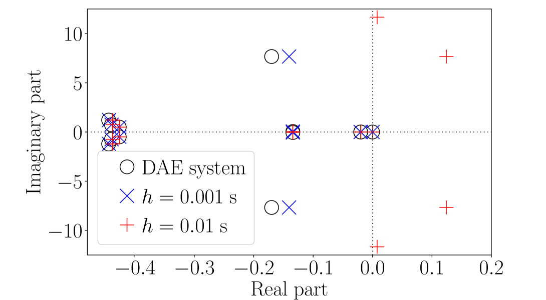
(a) FEM.

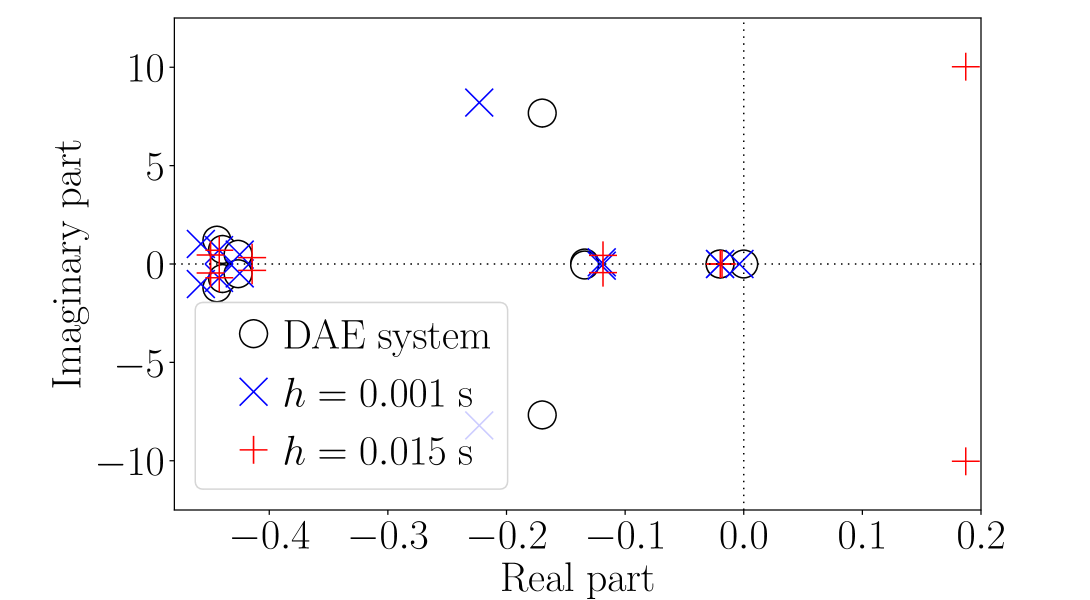
(b) RK4.

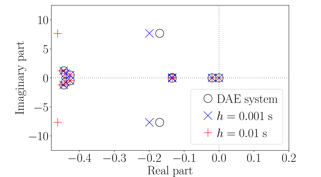
(c) BEM.

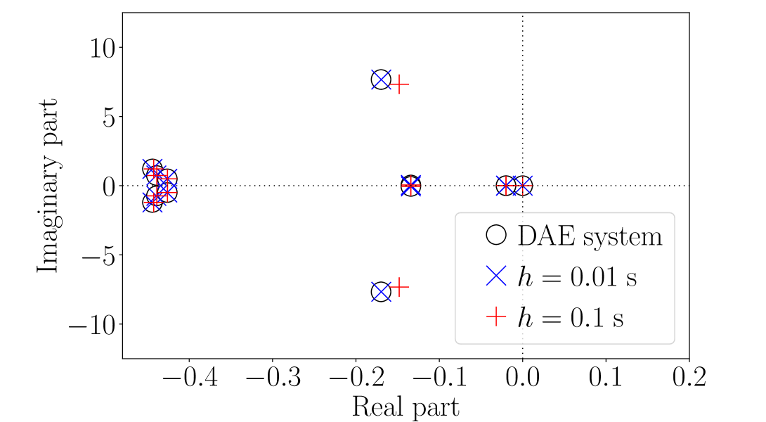
(d) ITM.

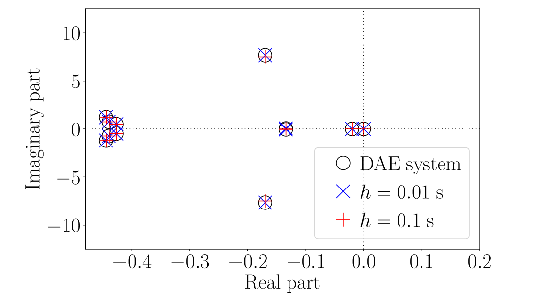
(e) 2S-DIRK.

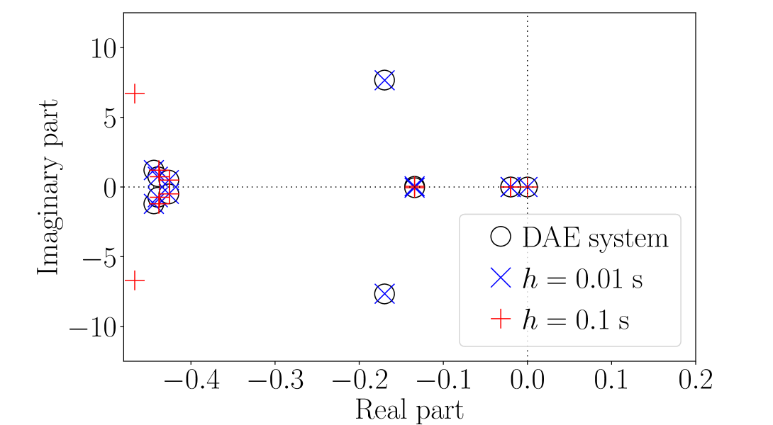
(f) BDF2.

Figure 1: WSCC system: Eigenvalue analysis of numerical TDI methods.

IV Case Studies

The simulation results provided in this section illustrate important features of the proposed framework to study the stability and accuracy of numerical methods applied for the TDI of power systems. The case study in Section IV-A is based on the well-known WSCC $9$-bus system [21], whereas Section IV-B considers a realistic model of the AIITS.

Simulations are carried out using Dome [22]. The version of Dome employed in this paper depends on ATLAS 3.10.3 for dense vector/matrix operations; CVXOPT 1.2.5 for sparse matrix operations; and KLU 1.3.9 for sparse matrix factorizations. The eigenvalues of matrix pencils are calculated using LAPACK [23]. All simulations are executed on a 64-bit Linux operating system running on 2 quad-core Intel Xeon 3.5 GHz CPUs, and 12 GB of RAM.

IV-A WSCC 9-Bus System

This section presents simulation results based on the WSCC $9$-bus system. The system comprises 6 transmission lines and 3 medium voltage/high voltage transformers; 3 Synchronous Generators represented by fourth-order, two-axis models and equipped with Turbine Governors and Automatic Voltage Regulators. In transient conditions, loads are modeled as constant admittances. In total, the system’s DAE model includes $39$ state and $57$ algebraic variables.

The small-disturbance dynamics of the system are represented by the eigenvalues of the pencil $s\boldsymbol{\rm E}-\boldsymbol{\rm A}$. Eigenvalue analysis shows that the system is stable when subjected to small disturbances, with the fastest and slowest dynamics represented by the real eigenvalues $-1000$ and $-0.02$, respectively, which gives a stiffness ratio $\mathcal{S}=5\cdot 10^{4}$.

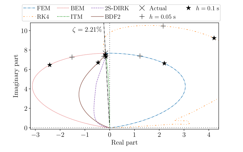
(a) Root locus.

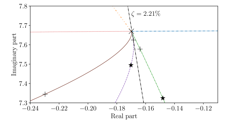
(b) Root locus (close-up).

Figure 2: WSCC system dominant mode: Root locus of numerical approximation as the time step is increased.

We consider the six numerical methods discussed in Section III-B. For each method, we calculate the associated pencil $\tilde{z}\,\tilde{\boldsymbol{\rm E}}-\tilde{\boldsymbol{\rm A}}$ and its eigenvalues, which are then mapped to the $S$-plane according to (18) and compared to the eigenvalues of $s\boldsymbol{\rm E}-\boldsymbol{\rm A}$. The comparison results for different time step sizes are presented in Fig. 1. As expected, for a sufficiently large $h$ the explicit methods are destabilized. Varying $h$ allows determining the maximum time step before numerical stability is lost. In particular, the time step margin of the FEM and the RK4 for the WSCC system are obtained as $0.005$ s and $0.011$ s, respectively. For larger time steps, there is at least one dynamic mode for which $\alpha<0$ and $\tilde{\alpha}>0$ in (19) and thus any TDI executed with such step values is guaranteed to diverge. The figure also shows that both the BEM and the BDF2 overdamp the dynamics of the system, which is again as expected. In addition, varying $h$ allows estimating the upper time step bound for which the overdamping is less than a certain prescribed degree. For instance, if it is required that the overdamping of all dynamic modes of the system is less than $d_{\zeta}=1$% (see also eq. (20)), then the upper bounds of $h$ for the BEM and BDF2 are $0.002$ s and $0.051$ s, respectively. Finally, among all methods considered, the 2S-DIRK shows the highest accuracy, while the ITM also shows very good accuracy for time steps smaller than $10^{-1}$ s. We focus on the dominant dynamic mode of the system, i.e. the local electromechanical oscillation of the SG connected to bus 2. In the eigenvalue analysis, this mode is represented by the complex pair $-0.1699\pm\jmath 7.6696$ with damping ratio $2.21$%. The root loci in Fig. 2 illustrate the accuracy of the TDI methods in approximating the mode as $h$ increases. The figure shows the route of explicit methods towards instability as well as of hyperstable methods to overdamped regions. From the close-up shown in Fig. 2(b), it is seen that, interestingly, the RK4 introduces a slight overdamping for small enough step sizes. Comparing the ITM with the 2S-DIRK, which are both symmetrically A-stable, we see that under the same step the 2S-DIRK is more accurate. In addition, for steps smaller than $0.05$ s, the 2S-DIRK follows precisely the mode’s damping, whereas for larger steps, it introduces a slight overdamping. On the other hand, the ITM underdamps the mode, which for a large enough $h$ leads to sustained numerical oscillations. For the sake of example, Table I gives the damping distortion $d_{\zeta}$ introduced by all methods for $h=0.05$ s. Finally, as $h$ increases, the distorted eigenvalue approaches zero for all methods. This is consistent with (18), whereby substituting the limit case $h\rightarrow\infty$, one has $\tilde{s}_{k}\rightarrow 0$.

TABLE I: WSCC system dominant mode: Damping distortion for $h=0.05$ s; and time step leading to $|d_{s}|=0.1$.

	FEM	RK4	BEM	ITM	2S-DIRK	BDF2
$d_{\zeta}$ [%]	-18.5	-22.4	18.2	-0.052	-0.005	0.9
($h=0.05$ s)
$h$ [s]	0.003	0.0002	0.003	0.052	0.075	0.026
($|d_{s}|=0.1$)

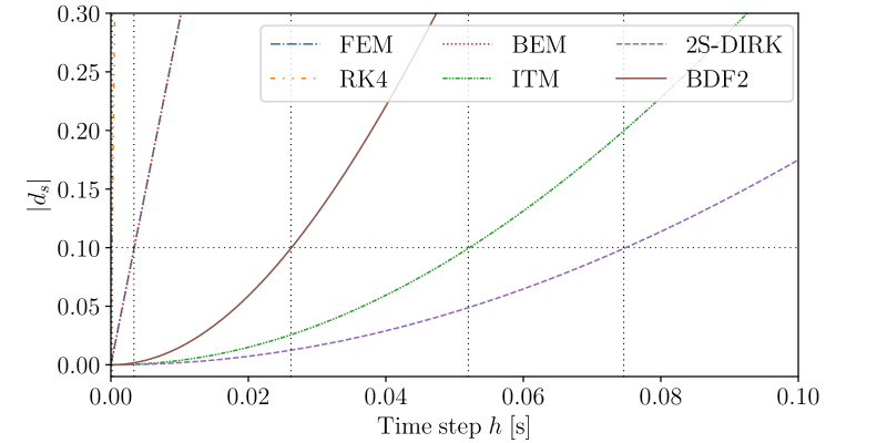
Figure 3: Dominant mode of WSCC system: Magnitude of numerical distortion.

For the same mode, the magnitude of numerical distortion as a function of $h$ is depicted in Fig. 3. The BEM and the FEM, being the former the implicit version of the latter, cause practically the same amount of distortion for every $h$, yet in opposite directions, with the BEM leading to overdamping and the FEM to instability (see Fig. 2(a)). Figure 3 allows determining the time step that introduces a certain amount of numerical distortion to the mode. For example, the time step of each method leading to $|d_{s}|=0.1$ is given in Table I.

In the remainder of this section, we focus exclusively on implicit methods, i.e. further simulation results are provided for the BEM, ITM, 2S-DIRK and BDF2. We carry out a non-linear time domain simulation considering a three-phase short-circuit at bus 5. The fault occurs at $t=1$ s and is cleared after $80$ ms by tripping the line that connects buses 5 and 7. The system is integrated using $h=0.05$ s. The response of the rotor speed of the SG at bus 2 ($\omega_{{\rm r},2}$), i.e., of the variable mostly participating to the dominant system mode, is shown in Fig. 4. For comparison, we have included a reference trajectory which represents an accurate integration of the system. The trajectories in Fig. 4 are consistent with the results of Table I, confirming that the small-disturbance analysis results provide a rough yet accurate estimation of the damping distortion introduced by TDI methods during the simulation. Considering the same disturbance, we simulate the system with the values of $h$ that correspond to $|d_{s}|=0.1$ of the dominant mode, as obtained in Table I. The response of the rotor speed of the SG at bus 2 in this case is shown in Fig. 5. As expected, integrating the system under a certain magnitude of numerical distortion leads to similar trajectories for all methods. Yet, the trajectories present some differences, since the distortion of each method is not in the same direction with the others (see e.g. Fig. 2). For example, the oscillation obtained with the BEM appears to be the most suppressed since the direction of its distortion introduces the largest overdamping.

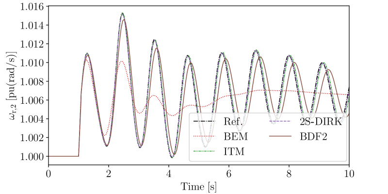
Figure 4: WSCC system: $\omega_{{\rm r},2}$ after the fault at bus 5, $h=0.05$ s.

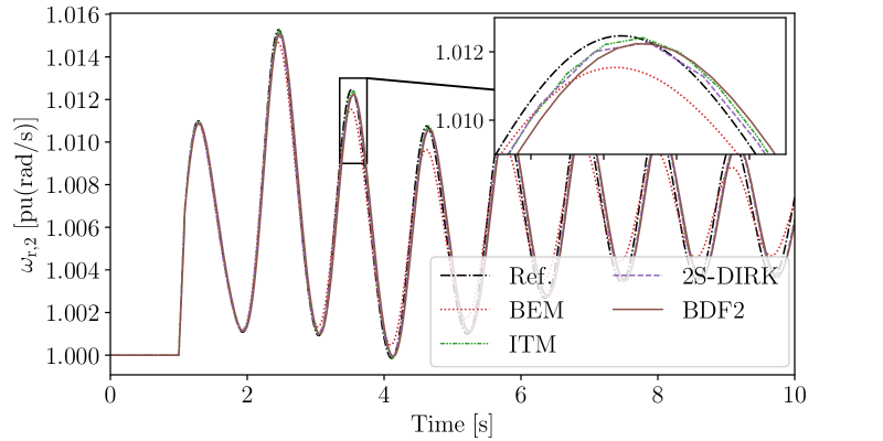
Figure 5: WSCC system: $\omega_{{\rm r},2}$ after the fault at bus 5, $|d_{s}|=0.1$.

IV-B All-Island Irish Transmission System

This section provides simulation results on a $1,479$-bus model of the AIITS. The topology and steady-state operation data of the system have been provided by the Irish transmission system operator, EirGrid Group. Dynamic data have been determined based on current knowledge about the technology of generators and controllers. The system comprises $796$ lines, $1,055$ transformers, $245$ loads, $22$ SGs, with AVRs and TGs, $6$ power system stabilizers and $176$ wind generators. The model has $1,443$ state and $7,197$ algebraic variables.

TABLE II: AIITS: Cumulative $\omega_{{\rm r},2}$ trajectory mismatches introduced by TDI methods, $h=0.1$ s.

Oper. point	Disturbance	BEM	ITM	2S-DIRK	BDF2
Base case	SG outage	$1.8\cdot 10^{-2}$	$4.3\cdot 10^{-4}$	$2.0\cdot 10^{-4}$	$8.8\cdot 10^{-3}$
	Load trip	$6.4\cdot 10^{-3}$	$2.2\cdot 10^{-3}$	$1.2\cdot 10^{-4}$	$2.2\cdot 10^{-3}$
	3-phase fault	$8.7\cdot 10^{-3}$	$2.7\cdot 10^{-3}$	$1.3\cdot 10^{-3}$	$9.0\cdot 10^{-3}$
	EWIC trip	$2.5\cdot 10^{-2}$	$1.1\cdot 10^{-3}$	$5.4\cdot 10^{-4}$	$1.2\cdot 10^{-2}$
$+5$% load	SG outage	$5.4\cdot 10^{-1}$	$5.6\cdot 10^{-2}$	$5.5\cdot 10^{-2}$	$7.3\cdot 10^{-2}$
	Load trip	$1.0\cdot 10^{-1}$	$1.7\cdot 10^{-2}$	$8.2\cdot 10^{-3}$	$4.3\cdot 10^{-2}$
	3-phase fault	$3.2\cdot 10^{-1}$	$4.4\cdot 10^{-2}$	$3.3\cdot 10^{-2}$	$1.8\cdot 10^{-1}$
	EWIC trip	$4.6\cdot 10^{-2}$	$1.2\cdot 10^{-2}$	$6.0\cdot 10^{-3}$	$3.9\cdot 10^{-2}$
$-5$% load	SG outage	$1.8\cdot 10^{-2}$	$6.7\cdot 10^{-4}$	$3.1\cdot 10^{-4}$	$9.0\cdot 10^{-3}$
	Load trip	$5.5\cdot 10^{-3}$	$2.0\cdot 10^{-3}$	$1.1\cdot 10^{-4}$	$2.0\cdot 10^{-3}$
	3-phase fault	$4.2\cdot 10^{-2}$	$1.3\cdot 10^{-2}$	$6.4\cdot 10^{-3}$	$4.3\cdot 10^{-2}$
	EWIC trip	$1.2\cdot 10^{-1}$	$5.7\cdot 10^{-3}$	$3.7\cdot 10^{-3}$	$5.9\cdot 10^{-2}$

Eigenvalue analysis shows that the system is stable around the examined equilibrium point. The fastest and slowest dynamic modes have exponential decay rates $-99,900.1$ and $-0.077$, respectively, and thus the stiffness ratio of the model is $\mathcal{S}=1.3\cdot 10^{6}$. We consider the most poorly damped electromechanical mode of the system, i.e., the local oscillation of the SG connected to bus $507$. In the eigenvalue analysis results, this mode is represented by the complex pair $-0.3042\pm\jmath 4.1426$ with damping ratio $7.32$%. Hereafter, we will refer to this mode as MCEM (Most Critical Electromechanical Mode). The magnitude of numerical distortion of the damping of the MCEM as a function of $h$ for the BEM, ITM, 2S-DIRK and BDF2 is shown in Fig. 6.

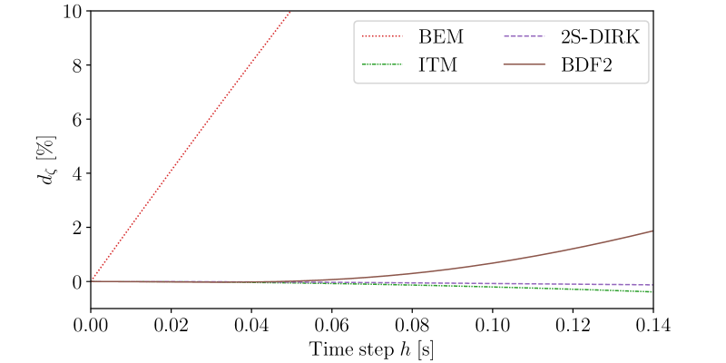
Figure 6: AIITS: Damping distortion $d_{\zeta}$, MCEM.

TABLE III: AIITS: Time step for $|d_{s}|=0.1$, MCEM.

	BEM	ITM	2S-DIRK	BDF2
$h$ [s]	0.011	0.131	0.189	0.066

The time steps that correspond to $|d_{s}|=0.1$ for the MCEM are given in Table III. Using these time step values we provide a comparison of the four implicit numerical methods by executing a non-linear TDI, assuming the loss of the SG connected to bus 684 at $t=1$ s. The response of the rotor speed of the SG at bus 507 following the disturbance is shown in Fig. 7. As expected, all methods provide a similar response and a small deviation from the reference trajectory. The trajectory obtained with the BEM appears to be more damped than the others, which was also to be expected (see Section IV-A).

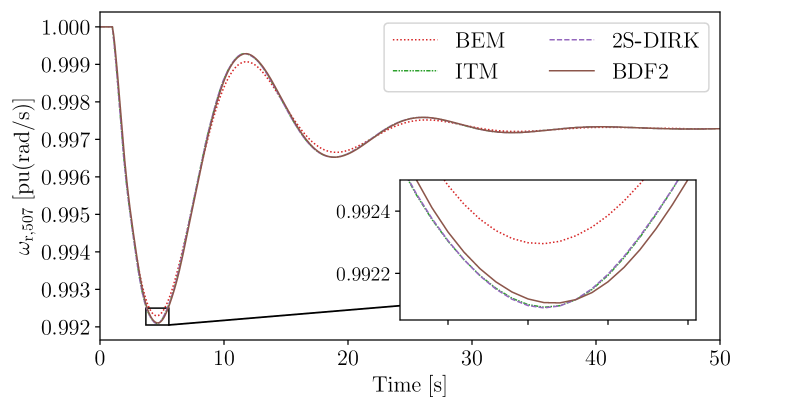
Figure 7: AIITS: $\omega_{{\rm r},2}$ after SG outage, $|d_{s}|=0.1$ (MCEM).

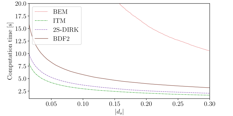
Figure 8: AIITS: $|d_{s}|$ of MCEM vs TDI total computation time.

A relevant remark is that evaluating different methods under the same amount of numerical distortion can be employed as a means for their fair computational comparison. As an example, for each implicit TDI method we vary $|d_{s}|$ for the MCEM and for every value we calculate the corresponding time step $h$. Using this step value we integrate the system and compute the computational time required to complete the simulation.

The results shown in Fig. 7 indicate that, for the examined scenario, the ITM is the method that takes the lowest total computational time. Yet, as $|d_{s}|$ increases, the relative difference of the ITM with respect to the other methods decreases. For large time steps, in fact, the ITM shows large sustained numerical oscillations which in turn lead to an increased number of required iterations per step, while the opposite is true for the methods that introduce overdamping, i.e., they require less iterations.

We note that considering a single dynamic mode is assumed in Figs. 3 and 6 for the sake of simplicity, but this is not a limitation of the proposed approach, since the analysis can be extended to take into account a group of critical modes, or even all system modes.

Finally, in addition to the operating condition assumed so far in this example (base case), we consider two more. The new operating conditions are obtained through a $137$ MW load increase/decrease (corresponding to $5$% increase/decrease of the system’s total power consumption). For each operating condition, we consider four different disturbances, (i) outage of $90$ MW synchronous generation at bus 684, (ii) loss of a total of $101.4$ MW power consumption connected to buses 1-5, (iii) three-phase fault at bus 1238, cleared by tripping a transmission line connected to the faulted bus after $100$ ms. (iv) loss of the VSC-HVDC link East-West Inter-connector (EWIC) that connects the AIITS to Great Britain’s transmission system.

The system is integrated with the BEM, the ITM, the 2S-DIRK, and the BDF2, for $15$ s and using $h=0.1$ s. In every simulation, the disturbance is applied at $t=1$ s. Table II shows, for each method and scenario, the magnitude of the error of the rotor speed $\omega_{{\rm r},2}$ with respect to the reference trajectory, cumulated for the simulation period. Moreover, the values of $|d_{s}|$ for the mode to which $\omega_{{\rm r},2}$ mostly participates in, i.e. the MCEM, are given in Table IV. The values in Table IV are determined considering the base case operating condition. Results further confirm the suitability of the proposed approach in providing indicative and useful, yet not absolute measures of the numerical distortion introduced by TDI methods. Of course, repeating the SSSA when the operating condition is varied, would allow a further improvement of the precision of the measures derived.

TABLE IV: AIITS: $|d_{s}|$ for $h=0.1$ s, MCEM.

	BEM	ITM	2S-DIRK	BDF2
$|d_{s}|$	0.810	0.058	0.029	0.208

Overall, results support the validity of the proposed approach in providing indicative accuracy measures for the non-linear system model.

V Conclusions

The paper provides a framework based on SSSA to study the numerical distortion introduced by explicit and implicit integration schemes when applied for the simulation of power system dynamics. The proposed framework is implemented using a general formulation which covers the most important families of integration methods, including RK and linear multistep methods. Results indicate that adopting the proposed approach, one is able to provide useful upper time step bounds to satisfy certain accuracy criteria, as well as to compare different methods in a fair way.

Future work will exploit the proposed framework to provide new insights on the accuracy of multirate methods, e.g. see [24, 25, 26], as well as to evaluate the ability and limitations of common integration schemes to accurately cope with time delays and stochastic processes.

Appendix A Proofs of Propositions

A-A Proof of Proposition 1

We consider (16) and for simplicity we use the notation $\frac{\partial\boldsymbol{\eta}}{\partial\mbox{$\boldsymbol{\rm x}$}_{t}}=\boldsymbol{\rm A}_{0}$, $\frac{\partial\boldsymbol{\eta}}{\partial\mbox{$\boldsymbol{\rm x}$}_{t-h}}\boldsymbol{\rm A}_{h}$, $\frac{\partial\boldsymbol{\eta}}{\partial\mbox{$\boldsymbol{\rm x}$}_{t-a_{1}h}}=\boldsymbol{\rm A}_{a_{1}h}$, $\frac{\partial\boldsymbol{\eta}}{\partial\mbox{$\boldsymbol{\rm x}$}_{t-a_{2}h}}=\boldsymbol{\rm A}_{a_{2}h}$, $\ldots$, $\frac{\partial\boldsymbol{\eta}}{\partial\mbox{$\boldsymbol{\rm x}$}_{t-a_{\rho}h}}=\boldsymbol{\rm A}_{a_{\rho}h}.$ Let also $\epsilon>0$, so that $a_{i}=c_{i}\epsilon$, $c_{i}\in\mathbb{N}^{*}$. We set:

$$\boldsymbol{y}_{t}^{[0]} =\Delta\mbox{$\boldsymbol{\rm x}$}_{t}$$

$$\boldsymbol{y}_{t}^{[h]} =\Delta\mbox{$\boldsymbol{\rm x}$}_{t-h}$$

$$\vdots$$

$$\boldsymbol{y}_{t}^{[a_{1}h]} =\Delta\mbox{$\boldsymbol{\rm x}$}_{t-a_{1}h}$$

$$\boldsymbol{y}_{t}^{[(a_{1}+\epsilon)h]} =\Delta\mbox{$\boldsymbol{\rm x}$}_{t-(a_{1}+\epsilon)h}$$

$$\boldsymbol{y}_{t}^{[(a_{1}+2\epsilon)h]} =\Delta\mbox{$\boldsymbol{\rm x}$}_{t-(a_{1}+2\epsilon)h}$$

$$\vdots$$

$$\boldsymbol{y}_{t}^{[a_{2}h]} =\Delta\mbox{$\boldsymbol{\rm x}$}_{t-a_{2}h}$$

$$\boldsymbol{y}_{t}^{[(a_{2}+\epsilon)h]} =\Delta\mbox{$\boldsymbol{\rm x}$}_{t-(a_{2}+\epsilon)h}$$

$$\vdots$$

$$\boldsymbol{y}_{t}^{[a_{\rho-1}h]} =\Delta\mbox{$\boldsymbol{\rm x}$}_{t-a_{\rho-1}h}\,.$$

and

$$\boldsymbol{y}_{t-h}^{[0]} =\Delta\mbox{$\boldsymbol{\rm x}$}_{t-h}=\boldsymbol{y}_{t}^{[h]}$$

$$\boldsymbol{y}_{t-h}^{[h]} =\Delta\mbox{$\boldsymbol{\rm x}$}_{t-2h}=\boldsymbol{y}_{t}^{[2h]}$$

$$\boldsymbol{y}_{t-h}^{[2h]} =\Delta\mbox{$\boldsymbol{\rm x}$}_{t-3h}=\boldsymbol{y}_{t}^{[3h]}$$

$$\vdots$$

$$\boldsymbol{y}_{t-h}^{[a_{1}h]} =\Delta\mbox{$\boldsymbol{\rm x}$}_{t-(a_{1}+\epsilon)h}=\boldsymbol{y}_{t}^{[(a_{1}+\epsilon)h]}$$

$$\boldsymbol{y}_{t-h}^{(a_{1}+\epsilon)h} =\Delta\mbox{$\boldsymbol{\rm x}$}_{t-(a_{1}+2\epsilon)h}=\boldsymbol{y}_{t}^{[(a_{1}+2\epsilon)h]}$$

$$\vdots$$

$$\boldsymbol{y}_{t-h}^{[a_{2}h]} =\Delta\mbox{$\boldsymbol{\rm x}$}_{t-(a_{2}+\epsilon)h}=\boldsymbol{y}_{t}^{[(a_{2}+\epsilon)h]}$$

$$\boldsymbol{y}_{t-h}^{[(a_{2}+\epsilon)h]} =\Delta\mbox{$\boldsymbol{\rm x}$}_{t-(a_{2}+2\epsilon)h}=\boldsymbol{y}_{t}^{[(a_{1}+2\epsilon)h]}$$

$$\vdots$$

$$\boldsymbol{\rm A}_{a_{\rho}h}\boldsymbol{y}_{t-h}^{[a_{\rho-1}h]} =\boldsymbol{\rm A}_{a_{\rho}h}\Delta\mbox{$\boldsymbol{\rm x}$}_{t-a_{\rho}h}\,.$$

The last matrix equation can be written as:

$$\boldsymbol{\rm A}_{a_{\rho}h}\boldsymbol{y}_{t-h}^{[a_{\rho-1}h]}= -\boldsymbol{\rm A}_{0}\Delta\mbox{$\boldsymbol{\rm x}$}_{t}-\boldsymbol{\rm A}_{h}\Delta\mbox{$\boldsymbol{\rm x}$}_{t-h}-\boldsymbol{\rm A}_{a_{1}h}\Delta\mbox{$\boldsymbol{\rm x}$}_{t-a_{1}h}$$

$$-\ldots-\boldsymbol{\rm A}_{a_{\rho-1}h}\Delta\mbox{$\boldsymbol{\rm x}$}_{t-a_{\rho-1}h}\,.$$ (43)

or, equivalently,

$$\boldsymbol{\rm A}_{a_{\rho}h}\boldsymbol{y}_{t-h}^{[a_{\rho-1}h]}= -\boldsymbol{\rm A}_{0}\boldsymbol{y}_{t}^{[0]}-\boldsymbol{\rm A}_{h}\boldsymbol{y}_{t}^{[h]}-\boldsymbol{\rm A}_{a_{1}h}\boldsymbol{y}_{t}^{[a_{1}h]}$$

$$-\ldots-\boldsymbol{\rm A}_{a_{\rho-1}h}\boldsymbol{y}_{t}^{[a_{\rho-1}h]}\,.$$ (44)

Using the above matrix equations we arrive to system (17) which is equivalent to (16), where:

$$\tilde{\boldsymbol{\rm E}}=\left[\begin{array}[]{cc}\boldsymbol{\rm I}&\boldsymbol{\rm 0}\\ \boldsymbol{\rm 0}&\boldsymbol{\rm A}_{a_{\rho}h}\end{array}\right]\,,$$ (47)

$$\tilde{\boldsymbol{\rm A}}=\left[\begin{array}[]{cc}\boldsymbol{\rm 0}&\boldsymbol{\rm I}\\ -\boldsymbol{\rm A}_{0}&\boldsymbol{\rm A}^{\dagger}\end{array}\right]\,,$$ (50)

and:

$$\boldsymbol{\rm A}^{\dagger}=\left[\begin{array}[]{cccccccc}-\boldsymbol{\rm A}_{h}&\boldsymbol{\rm 0}&\dots-\boldsymbol{\rm A}_{a_{1}h}&\boldsymbol{\rm 0}&\dots&-\boldsymbol{\rm A}_{a_{\rho-1}h}&\boldsymbol{\rm 0}\end{array}\right]\,,$$

where $\boldsymbol{\rm 0}$, $\boldsymbol{\rm I}$ are the zero and identity matrix with proper dimensions.

$$\boldsymbol{\rm y}_{t}^{\scriptscriptstyle\rm T}= [(\boldsymbol{y}_{t}^{[0]})^{\scriptscriptstyle\rm T}\ \ \ (\boldsymbol{y}_{t}^{[h]})^{\scriptscriptstyle\rm T}\ \ \ (\boldsymbol{y}_{t}^{[2h]})^{\scriptscriptstyle\rm T}\ \ \dots\ \ (\boldsymbol{y}_{t}^{[a_{1}h]})^{\scriptscriptstyle\rm T}$$ (51)

$$(\boldsymbol{y}_{t}^{[(a_{1}+\epsilon)h]})^{\scriptscriptstyle\rm T}\ \ \dots\ \ (\boldsymbol{y}_{t}^{[a_{2}h]})^{\scriptscriptstyle\rm T}\ \ \ (\boldsymbol{y}_{t}^{[(a_{2}+\epsilon)h]})^{\scriptscriptstyle\rm T}$$

$$\ \ \dots\ \ (\boldsymbol{y}_{t}^{[a_{\rho-1}h]})^{\scriptscriptstyle\rm T}]\,.$$

Then, we have that the pencils $s^{a_{\rho}h}\boldsymbol{\rm A}_{a_{\rho}h}+\ldots+s^{a_{2}h}\boldsymbol{\rm A}_{a_{2}h}+s^{a_{1}h}\boldsymbol{\rm A}_{a_{1}h}+s^{h}\boldsymbol{\rm A}_{h}+\boldsymbol{\rm A}_{0}$, $s\tilde{\boldsymbol{\rm E}}-\tilde{\boldsymbol{\rm A}}$ of systems (16), (17) respectively, have exactly the same finite eigenvalues, see [9]. The proof is completed.

A-B Propositions 53 and 56

Proposition 2.

Recall the general form of the Möbius transformation [27]:

$$s=\frac{az+b}{cz+d}\,,\quad a,b,c,d\in\mathbb{C},\quad ad-bc\neq 0\,.$$ (52)

If (52) is applied to the matrix pencil $s\boldsymbol{\rm E}-\boldsymbol{\rm A}$, it leads to the family of pencils:

$$z(a\boldsymbol{\rm E}-c\boldsymbol{\rm A})-(d\boldsymbol{\rm A}-b\boldsymbol{\rm E})\,.$$ (53)

Proof.

First, the restriction $ad-bc\neq 0$ in (52) is necessary since, if $ad=bc$ then $s$ is constant, which is not possible. Then, recall that the eigenvalues of the pencil of (7) are the solutions of (8), whereby applying (52) we get:

$${\rm det}\Big{(}\frac{az+b}{cz+d}\boldsymbol{\rm E}-\boldsymbol{\rm A}\Big{)}=0\,,$$

or, equivalently, by using determinant properties:

$${\rm det}((a\boldsymbol{\rm E}-c\boldsymbol{\rm A})z-(d\boldsymbol{\rm A}-b\boldsymbol{\rm E}))=0\,,$$

i.e. the characteristic equation of a linear system with pencil:

$$z(a\boldsymbol{\rm E}-c\boldsymbol{\rm A})-(d\boldsymbol{\rm A}-b\boldsymbol{\rm E})\,.$$ (54)

The proof is completed. Then, we may obtain as special cases the matrix pencils of the FEM, for $a=1$, $b=-1$, $c=0$, $d=h$; the BEM, for $a=1$, $b=-1$, $c=h$, $d=0$; the ITM, for $a=1$, $b=-1$, $c=0.5h$, $d=0.5h$.

Note that the family of pencils (53) corresponds to a family of linear discrete-time systems in the form:

$$(a\boldsymbol{\rm E}-c\boldsymbol{\rm A})\Delta\mbox{$\boldsymbol{\rm x}$}_{t}=(d\boldsymbol{\rm E}-b\boldsymbol{\rm A})\Delta\mbox{$\boldsymbol{\rm x}$}_{t-h}\,.$$ (55)

Proposition 3.

Consider system (7) with $ad-bc\neq 0$. If one of the following conditions holds:

$$a=b\ \text{and}\ c=-d\,,\quad\text{or}\quad a=-b\ \text{and}\ c=d\,,$$ (56)

then for a stable equilibrium state of (7), the magnitude of the spectral radius of the matrix pencil of each discrete-time system in the form of (55) is $<1$.

Proof.

For a stable equilibrium state of (7), we have ${\rm Re}(s)<0$, for every finite eigenvalue $s\in\mathbb{C}$ and hence $s+\bar{s}<0$, where $\bar{s}$ is the complex conjugate of $s$. Substituting $s={(az+b)}/({cz+d})$ we get:

$$\frac{az+b}{cz+d}+\frac{a\bar{z}+b}{c\bar{z}+d}<0\,,$$

or, equivalently:

$$(c\bar{z}+d)(az+b)+(a\bar{z}+b)(cz+d)<0\,,$$

or, equivalently, by taking into account that $\bar{z}z=|z|^{2}$:

$$2ac|z|^{2}+2bd+(ad+bc)(\bar{z}+z)<0\,,$$

This means that the set $\{{\rm Re}(s)<0,\ \forall s\in\mathbb{C}\}$ maps to the set $\{ac|z|^{2}+bd+(ad+bc){\rm Re}(z)<0,\ \forall z\in\mathbb{C}\}$. If we apply conditions (56), we have $ac+bd=0$ and $ad+bc=0$ which is equal to ${bd}/{ac}=-1$. Hence, the above relation takes the form:

$$2ac|z|^{2}<-2bd\,,$$

and consequently $|z|<1$. Thus, through (7) and under the conditions (56), the set $\{{\rm Re}(s)<0,\ \forall s\in\mathbb{C}\}$ maps to the set $\{|z|<1,\ \forall z\in\mathbb{C}\}$ and consequently the stability of this continuous time system can be studied through the stability of the discrete-time system (55). Hence for a stable equilibrium state of (7), we obtain that the magnitude of the spectral radius of the pencil of each discrete-time system in the form of (55) is $<1$. The proof is completed.

Georgios Tzounas (M’21) received the Diploma (M.E.) degree in Electrical and Computer Engineering from the National Technical Univ. of Athens, Greece, in 2017, and the Ph.D. degree in Electrical Engineering from Univ. College Dublin (UCD), Ireland, in 2021. From Jan. to Apr. 2020, he was a Visiting Researcher at Northeastern Univ., Boston, MA. He is currently a Senior Power Systems Researcher at UCD, working on the EU H2020 project “EdgeFLEX”. His research interests include modelling, stability analysis and control of power systems.

Ioannis Dassios received his Ph.D. in Applied Mathematics from the Dpt of Mathematics, Univ. of Athens, Greece, in 2013. He worked as a Postdoctoral Research and Teaching Fellow in Optimization at the School of Mathematics, Univ. of Edinburgh, UK. He also worked as a Research Associate at the Modelling and Simulation Centre, University of Manchester, UK, and as a Research Fellow at MACSI, Univ. of Limerick, Ireland. He is currently a UCD Research Fellow at UCD, Ireland.

Federico Milano (F’16) received from the University of Genoa, Italy, the ME and Ph.D. in Electrical Engineering in 1999 and 2003, respectively. From 2001 to 2002, he was with the Univ. of Waterloo, Canada. From 2003 to 2013, he was with the Univ. of Castilla-La Mancha, Spain. In 2013, he joined the Univ. College Dublin, Ireland, where he is currently Professor of Power Systems Control and Protections and Head of Electrical Engineering. His research interests include power systems modeling, control and stability analysis.

References

- [1] B. Stott, “Power system dynamic response calculations,” Proceedings of the IEEE, vol. 67, no. 2, pp. 219–241, Feb. 1979.
- [2] H. W. Dommel and N. Sato, “Fast transient stability solutions,” IEEE Transactions on Power Apparatus and Systems, vol. PAS-91, no. 4, pp. 1643–1650, 1972.
- [3] J. Marti and J. Lin, “Suppression of numerical oscillations in the EMTP power systems,” IEEE Transactions on Power Systems, vol. 4, no. 2, pp. 739–747, 1989.
- [4] J. Astic, A. Bihain, and M. Jerosolimski, “The mixed Adams-BDF variable step size algorithm to simulate transient and long term phenomena in power systems,” IEEE Transactions on Power Systems, vol. 9, no. 2, pp. 929–935, 1994.
- [5] J. Sanchez-Gasca, R. D’Aquila, W. Price, and J. Paserba, “Variable time step, implicit integration for extended-term power system dynamic simulation,” in Proceedings of Power Industry Computer Applications Conference, 1995, pp. 183–189.
- [6] T. Noda, K. Takenaka, and T. Inoue, “Numerical integration by the 2-stage diagonally implicit Runge-Kutta method for electromagnetic transient simulations,” IEEE Transactions on Power Delivery, vol. 24, no. 1, pp. 390–399, 2009.
- [7] D. Fabozzi and T. Van Cutsem, “Simplified time-domain simulation of detailed long-term dynamic models,” in Proceedings of the IEEE PES General Meeting, 2009, pp. 1–8.
- [8] C. Fu, J. D. McCalley, and J. Tong, “A numerical solver design for extended-term time-domain simulation,” IEEE Transactions on Power Systems, vol. 28, no. 4, pp. 4926–4935, 2013.
- [9] F. Milano, I. Dassios, M. Liu, and G. Tzounas, Eigenvalue Problems in Power Systems. CRC Press, Taylor & Francis Group, 2020.
- [10] M. Borodulin, “An approach to evaluating accuracy of numerical simulation of linear network transients,” in Proceedings of the Power Systems Computation Conference, Jun. 2002.
- [11] P. Kundur, Power System Stability and Control. New York: Mc-Grall Hill, 1994.
- [12] PSS/E 33.0, Program Application Guide Volume 2. Siemens, 2011.
- [13] G. Tzounas, I. Dassios, M. Liu, and F. Milano, “Comparison of numerical methods and open-source libraries for eigenvalue analysis of large-scale power systems,” Applied Sciences, vol. 10, no. 21, 2020.
- [14] J. D. Lambert et al., Numerical methods for ordinary differential systems. Wiley New York, 1991, vol. 146.
- [15] F. Bizzarri, A. Brambilla, and F. Milano, “The probe-insertion technique for the detection of limit cycles in power systems,” IEEE Transactions on Circuits and Systems I: Regular Papers, vol. 63, no. 2, pp. 312–321, 2016.
- [16] F. de Mello, J. Feltes, T. Laskowski, and L. Oppel, “Simulating fast and slow dynamic effects in power systems,” IEEE Computer Applications in Power, vol. 5, no. 3, pp. 33–38, 1992.
- [17] R. Scherer, “A necessary condition for B-stability,” BIT Numerical Mathematics, vol. 19, no. 1, pp. 111–115, 1979.
- [18] G. C. Verghese, I. J. Pérez-Arriaga, and F. C. Schweppe, “Selective modal analysis with applications to electric power systems, part ii: the dynamic stability problem,” IEEE Transactions on Power Apparatus and Systems, vol. PAS-101, no. 9, pp. 3126–3134, Sep. 1982.
- [19] J. H. Chow, Power System Coherency and Model Reduction, ser. Power Electronics and Power Systems 94. New York: Springer-Verlag, 2013.
- [20] G. Tzounas and F. Milano, “Delay-based decoupling of power system models for transient stability analysis,” IEEE Transactions on Power Systems, vol. 36, no. 1, pp. 464–473, 2021.
- [21] P. Sauer and M. Pai, Power System Dynamics and Stability. Prentice Hall, 1998.
- [22] F. Milano, “A Python-based software tool for power system analysis,” in Proceedings of the IEEE PES General Meeting, Jul. 2013.
- [23] E. Angerson, Z. Bai, J. Dongarra, A. Greenbaum, A. McKenney, J. D. Croz, S. Hammarling, J. Demmel, C. Bischof, and D. Sorensen, “LAPACK: A portable linear algebra library for high-performance computers,” in Proceedings of the ACM/IEEE Conference on Supercomputing, Nov. 1990, pp. 2–11.
- [24] D. Shu, X. Xie, Q. Jiang, G. Guo, and K. Wang, “A multirate EMT co-simulation of large AC and MMC-based MTDC systems,” IEEE Transactions on Power Systems, vol. 33, no. 2, pp. 1252–1263, 2017.
- [25] J. Chen and M. L. Crow, “A variable partitioning strategy for the multirate method in power systems,” IEEE Transactions on Power Systems, vol. 23, no. 2, pp. 259–266, 2008.
- [26] F. Moreira, J. Marti, L. Zanetta, and L. Linares, “Multirate simulations with simultaneous-solution using direct integration methods in a partitioned network environment,” IEEE Transactions on Circuits and Systems I: Regular Papers, vol. 53, no. 12, pp. 2765–2778, 2006.
- [27] I. Dassios, G. Tzounas, and F. Milano, “The Möbius transform effect in singular systems of differential equations,” Applied Mathematics and Computation, vol. 361, pp. 338–353, 2019.