Supporting Information: Quantum reality with negative-mass particles

Abstract

Quantum Physics, Weak Values, Quantum Paradoxes, Time-Symmetry, Quantum Measurement

I Strong and Weak Measurement

We begin with a review of the quantum measurement theory which gives rise to both the ABL rule in the limit of strong projective measurement, and the weak value in the limit of weak measurements. As we will see, the weak value becomes encoded into the pointer wavefunction of a measurement device when the translation induced by the coupling Hamiltonian is so small relative to the width of the pointer wavefunction that the different terms interfere — a weak measurement — and the ensemble is both pre- and post-selected.

We can model a general measurement by considering the position wavefunction of the pointer system as it is moved along some ruler by the measurement interaction. Let us consider the case that the pointer wavefunction is a Gaussian of width $\varepsilon$, and the ruler tick marks that indicate orthogonal states of the measured system are a distance $d$ apart. The usual case of a strong projective measurement is the case that $\varepsilon\ll d$, which means that the pointer has a very narrow peak, always centered on a tick mark of the ruler. The other extreme case where $\varepsilon\gg d$ is the regime of weak measurements, in which case each Gaussian is broadly spread around its ruler mark, and may overlap and interfere with Gaussian terms centered on other marks. If we consider a pre- and post-selected ensemble of weak measurements, this interference results in a Gaussian that is centered at the weak value (to first order in $d/\varepsilon$).

As an example, let us consider a measurement of a single spin-1/2 particle using a continuous Gaussian pointer. The impulsive coupling Hamiltonian between the spin and the pointer is given by,

$$\hat{H}=g(t)\sigma_{z}\hat{P}_{p},$$ (1)

where $\sigma_{z}=|0\rangle\langle 0|-|1\rangle\langle 1|$ is the Pauli operator of the qubit, $\hat{P}_{p}$ is the momentum operator of the pointer system, and $g(t)$ is the coupling strength. We will assume that the interaction lasts for only a very brief period $\tau$, and that during this time, we can neglect the systems’ other unitary evolution. This $g_{o}=\int_{0}^{\tau}g(t)dt$ is the relevant coupling parameter. The general initial state of the qubit is,

$$|\varphi_{0}\rangle=a|0\rangle+b|1\rangle,$$ (2)

which is expressed in the $\sigma_{z}$ basis, with $|a|^{2}+|b|^{2}=1$, and the initial wavefunction of the pointer is

$$\psi(x)=(\varepsilon^{2}\pi)^{-1/4}e^{-x^{2}/2\varepsilon^{2}}$$ (3)

The system and pointer begin in the product state,

$$|\Psi_{0}\rangle=|\varphi_{0}\rangle\int_{-\infty}^{\infty}\psi(x)|x\rangle dx.$$ (4)

After the interaction, the two systems are in the entangled state,

$$|\Psi\rangle=e^{-ig_{0}\sigma_{z}P_{p}/\hbar}|\Psi_{0}\rangle$$ (5)

$$=\left(a|0\rangle e^{-ig_{0}P_{p}/2}+b|1\rangle e^{ig_{0}P_{p}/2}\right)\int_{-\infty}^{\infty}\psi(x)|x\rangle dx$$

$$=\int_{-\infty}^{\infty}dx|x\rangle[a|0\rangle\psi(x-d)+b|1\rangle\psi(x+d)],$$

with $d=g_{0}$, which sets the scale of the ruler.

Now, suppose we project the qubit onto a general normalized state $|\varphi_{f}\rangle=\alpha|0\rangle+\beta|1\rangle$ (the post-selection).

First we consider the strong measurement limit $\varepsilon\rightarrow 0$, where $\psi(x)\rightarrow\sqrt{\delta(x)}$, and the renormalized wavefunction is,

$$\psi_{f}^{s}(x)=\big{(}\alpha^{*}a\sqrt{\delta(x-d)}+\beta^{*}b\sqrt{\delta(x+d)}\big{)}/\sqrt{|\alpha a|^{2}+|\beta b|^{2}}.$$ (6)

Taking the probability to find the pointer at positions $x=\pm d$, we obtain the ABL probability rule for finding eigenstate $|j\rangle$ ($j\in\{0,1\}$) when an intermediate strong projective measurement of $\sigma_{z}$ is made,

$$P_{\textrm{ABL}}(|j\rangle\langle j|=1\;|\;\varphi_{f},\varphi_{0},\sigma_{z})=\frac{|\langle\varphi_{f}|j\rangle\langle j|\varphi_{0}\rangle|^{2}}{\sum_{k\in\{0,1\}}|\langle\varphi_{f}|k\rangle\langle k|\varphi_{0}\rangle|^{2}}.$$ (7)

For a large PPS ensemble, the conditional expectation value of the intermediate measurement of $\sigma_{z}$,

$$\langle\hat{\sigma_{z}}\rangle_{ABL}=\sum_{j}\lambda_{j}P_{\textrm{ABL}}(|j\rangle\langle j|=1\;|\;\varphi_{f},\varphi_{0},\sigma_{z})$$ (8)

$$=P_{\textrm{ABL}}(|0\rangle\langle 0|=1\;|\;\varphi_{f},\varphi_{0},\sigma_{z})-P_{\textrm{ABL}}(|1\rangle\langle 1|=1\;|\;\varphi_{f},\varphi_{0},\sigma_{z})$$

$$=\frac{|\alpha a|^{2}-|\beta b|^{2}}{|\alpha a|^{2}+|\beta b|^{2}},$$

where $\lambda_{j}$ is the eigenvalue corresponding to eigenstate $|j\rangle$.

Next we consider the weak measurement regime where $\varepsilon\gg d$, the two $\psi$ terms explicitly interfere, and the renormalized pointer wavefunction is,

$$\psi_{f}^{w}(x)=\big{(}\alpha^{*}a\psi(x-d)+\beta^{*}b\psi(x+d)\big{)}/\langle\varphi_{f}|\varphi_{0}\rangle$$ (9)

$$=(\varepsilon^{2}\pi)^{-1/4}(\alpha^{*}ae^{-(x-d)^{2}/2\varepsilon^{2}}+\beta^{*}be^{-(x+d)^{2}/2\varepsilon^{2}})/\langle\varphi_{f}|\varphi_{0}\rangle$$

$$\approx(\varepsilon^{2}\pi)^{-1/4}e^{-(x^{2}+d^{2})/2\varepsilon^{2}}\bigg{(}\frac{\alpha^{*}a(1+xd/\varepsilon^{2})+\beta^{*}b(1-xd/\varepsilon^{2})}{\alpha^{*}a+\beta^{*}b}\bigg{)}$$

$$=(\varepsilon^{2}\pi)^{-1/4}e^{-(x^{2}+d^{2})/2\varepsilon^{2}}\left(1+\frac{\alpha^{*}a-\beta^{*}b}{\alpha^{*}a+\beta^{*}b}(xd/\varepsilon^{2})\right)$$

$$\approx(\varepsilon^{2}\pi)^{-1/4}\exp{\left(-\frac{1}{2\varepsilon^{2}}\left(x-d\left[\frac{\alpha^{*}a-\beta^{*}b}{\alpha^{*}a+\beta^{*}b}\right]\right)^{2}\right)}$$

$$=\psi(x-d(\sigma_{z})_{w}),$$

where,

$$(\sigma_{z})_{w}\equiv\frac{\langle\varphi_{f}|\sigma_{z}|\varphi_{0}\rangle}{\langle\varphi_{f}|\varphi_{0}\rangle}=\frac{\alpha^{*}a-\beta^{*}b}{\alpha^{*}a+\beta^{*}b},$$ (10)

is the weak value of $\sigma_{z}$ given the pre-selection $|\varphi_{0}\rangle$ and the post-selection $\langle\varphi_{f}|$. Note that the weak value has emerged from the interference of two Gaussian terms with complex coefficients coming from both the pre- and post-selection.

Let us contrast the two limits: In the strong case, the final pointer function is a superposition of two delta functions at $x=\pm d$, meaning one obtains a definite eigenvalue shot-by-shot, and the mean value $d\langle\hat{\sigma_{z}}\rangle_{ABL}$ emerges from a PPS ensemble. In the weak case, the final pointer function is a broad Gaussian, meaning one effectively obtains only noise shot-by-shot, and the mean value $d(\sigma_{z})_{w}$ emerges from a PPS ensemble.

As we have seen, the weak value emerges due to interference of the pointer, mediated (or steered) by entanglement with the measured system. Now, the initial pointer state had $\langle x\rangle_{0}=0$ and $\langle p\rangle_{0}=0$, and it is straightforward to check that the final pointer state has $\langle x\rangle_{f}=d\textrm{Re}[(\sigma_{z})_{w}]$ and $\langle p\rangle_{f}\approx d\hbar\textrm{Im}[(\sigma_{z})_{w})]/\varepsilon^{2}$, and thus we see that the real part of the weak value is proportional to the shift in the pointer position, while the imaginary part is proportional to the shift in the pointer momentum (to first order). This gives us a physical interpretation of the complex weak value.

The derivation above can be naturally generalized to measure any observable $\hat{A}$ on any physical system using the same pointer, and the Hamiltonian, $\hat{H}=g(t)\hat{A}\hat{P}_{p}$ to measure the weak value, $A_{w}$.

In the limit that $\varepsilon\gg d$, the weak value is the dominant effect on the pointer wavefunction, and as one takes the limit that $d/\varepsilon\rightarrow 0$, the weak value is always encoded in the pointer wavefunction, right down to the limit that there is no interaction at all. The premise of the weak value interpretation is that all of these weak values are physically existent properties of the system, whether or not we choose to weakly measure them. This is reminiscent of how the electric field is defined at each location by considering the limit that the magnitude of a test charge placed at that location goes to zero, whether or not we actually measure the force the field exerts on a charge at that location. In this picture, it is the weak values which describe how nature behaves when we are not looking, and the usual eigenvalues which describe how it behaves when we are.

II Resolving Paradoxes

Here we explore a number of PPS-scenarios and PPS-paradoxes and construct the relevant weak values. We then work out the top-down counterparticle description in the weak reality, and discuss the resolution of the corresponding paradoxes (if any) in the ABL interpretation.

II.1 The Disappearing and Reappearing Particle Paradox

The 3-box paradox can be generalized to a time-dependent case in an interesting way aharonov2017case . Suppose that a particle is pre-selected in the state $|\psi\rangle=(|1\rangle+\sqrt{2}|2\rangle)/\sqrt{3}$ at time $t=0$, and post-selected in the state $|\varphi\rangle=(|1\rangle-i\sqrt{2}|3\rangle)/\sqrt{3}$ at $t=2$. Boxes 2 and 3 share a wall that allows tunneling, while box 1 is isolated from both of them. Due to the tunneling, the amplitude of the wavefunction will oscillate back and forth between between the two boxes according to the unitary evolution matrix,

$$U(\Delta t)=\left(\begin{array}[]{ccc}1&0&0\\ 0&\cos(\pi\Delta t/4)&i\sin(\pi\Delta t/4)\\ 0&i\sin(\pi\Delta t/4)&\cos(\pi\Delta t/4)\\ \end{array}\right).$$ (11)

Using this expression we can propagate $|\psi\rangle$ forward and $|\varphi\rangle$ backward to an intermediate time $t$. This gives $|\psi_{t}\rangle=(|1\rangle+\sqrt{2}\cos(\pi t/4)|2\rangle+i\sqrt{2}\sin(\pi t/4)|3\rangle)/\sqrt{3}$ and $|\varphi_{t}\rangle=(|1\rangle+\sqrt{2}\sin(\pi t/4)|2\rangle-i\sqrt{2}\cos(\pi t/4)|3\rangle)/\sqrt{3}$, where we call $|\varphi_{t}\rangle$ the destiny vector. With these we can compute the weak value of each projector at time $t$ as, $|1_{t}|_{w}=1$, $|2_{t}|_{w}=\sin(\pi t/2)$, and $|3_{t}|_{w}=-\sin(\pi t/2)$.

Consider the weak value $|\Pi^{23}_{t}|_{w}=|2_{t}|_{w}+|3_{t}|_{w}=0$. According to the ABL interpretation, this should mean that there is never a particle in either of boxes 2 or 3, and thus the particle must be in box 1 at all times. However, at $t=1$, we have $|\Pi^{13}_{1}|_{w}=|1_{1}|_{w}+|3_{1}|_{w}=0$, meaning the particle must be in box 2, at $t=3$ we have $|\Pi^{12}_{3}|_{w}=|1_{3}|_{w}+|2_{3}|_{w}=0$, meaning the particle must be in box 3. At these two times, we have recovered exactly the original 3-box paradox. The added subtlety is that the particle seems to definitely be in box 1 at all times, but then at $t=1$ it seems paradoxically to also be in box 2, even though there is no tunneling between boxes 1 and 2, and likewise it seems to also be in box 3 at $t=3$.

The counterparticle ontology has a single positive particle in box 1 with probability 1, however the situation in boxes 2 and 3 is more complicated. At $t=0$ there probability 1/2 to find a positive particle in box 2 and a negative one in box 2, and also probability 1/2 to find them reversed - leading to weak value of 0. As time evolves, each of these starting configurations of counterparticles has some probability to flip due to tunneling, such that the total probability of finding the first configuration is $P_{+-}=[1-\sin(\pi t/2)]/2$ and the total probability to find the second is $P_{-+}=[1+\sin(\pi t/2)]/2$.

As this happens, the negative real particles can mask the positive real particles so that sometimes it looks as though a given box is empty, and in time it looks as though the positive-real particle in boxes 2 or 3 gradually disappears and then gradually reappears as a negative-real particle, only to reverse course, vanishing and reappearing as a positive particle before the entire process repeats.

Note that the total probability to find a negative particle in boxes 2 or 3 is always 1, as is the probability find a positive particle in boxes 2 or 3. Note also, that provided the pre-selected state at $t=0$ is $|\psi\rangle$, we can choose the post-selection $|\varphi_{t}\rangle$ at any time $t$ and the ontology is the same.

II.2 The Case of the Hollow Atoms

In the following thought experiment we will analyze another case of the 3-box paradox using tripartite system composed of two protons (hereby denoted by $p_{1}$,$p_{2}$) and one electron ($e$) superposed over 3 boxes. The electron is assumed to bind to either proton if they are left in the same box, thus forming a hydrogen atom. As we shall see, upon a particular choice of pre- and post-selected states, the weak reality will tell us a peculiar story.

The system is prepared in the state

$$|\psi\rangle=|1^{p_{1}}\rangle|1^{e}\rangle|3^{p_{2}}\rangle+|2^{p_{1}}\rangle|2^{e}\rangle|3^{p_{2}}\rangle+|2^{p_{1}}\rangle|3^{e}\rangle|3^{p_{2}}\rangle,$$ (12)

and post-selected in the state:

$$|\varphi\rangle=|1^{p_{1}}\rangle|1^{e}\rangle|3^{p_{2}}\rangle+|2^{p_{1}}\rangle|2^{e}\rangle|3^{p_{2}}\rangle-|2^{p_{1}}\rangle|3^{e}\rangle|3^{p_{2}}\rangle,$$ (13)

Both the pre- and post-selected states therefore represent the case where there is a hydrogen atom superposed over the three boxes and there is always a “spectator” proton, which is sometimes the separable proton in the third box and sometimes is the entangled proton in the second box.

The nonzero weak values of the rank-1 projectors are,

$|1^{p_{1}}1^{e}|_{w}=1$, $|2^{p_{1}}2^{e}|_{w}=1$, $|2^{p_{1}}3^{e}|_{w}=-1$ $|3^{p_{2}}|_{w}=1$, and the rank-2 projector weak values for $p_{1}$ are, $|1^{p_{1}}|_{w}=|1^{p_{1}}2^{e}|_{w}=1$, $|2^{p_{1}}|_{w}=|2^{p_{1}}2^{e}|_{w}+|2^{p_{1}}3^{e}|_{w}=0$, and for $e$ they are $|1^{e}|_{w}=|1^{p_{1}}1^{e}|_{w}=1$, $|2^{e}|_{w}=|2^{p_{1}}2^{e}|_{w}=1$, and $|3^{e}|_{w}=|2^{p_{1}}3^{e}|_{w}=-1$.

In terms of single-particle weak values, the second term in the pre- and post-selected states indicates the effective presence of a positive electron and a positive proton within the second box. However, the third term implies the effective presence of a proton counter-particle (i.e. the weak value of the corresponding projector is equal to $-1$). Therefore, in the weak reality, the proton particle and counter-particle effectively cancel and we seem to have in total just one electron within the second box. However, the two-particle weak value of the projector onto an electron-proton pair (henceforth an “atom”) within the second box is $|2^{p_{1}}2^{e}|_{w}=1$. We can thus interpret the ABL paradox here as implying that the electron in box 2 is bound to an empty nucleus, thus forming a ‘Hollow Atom.’

The top-down 2-structures and counterparticles of the weak value ontology of this case has a positive 2-structure with a $p_{1}$ and an $e$ in box 1, a positive 2-structure with a $p_{1}$ and an $e$ both in box 2, a negative 2-structure with a $p_{1}$ in box 2 and an $e$ in box 3, and single positive $p_{2}$ in box 3. This explains the weak values, and there is no paradox.

Remarkably, the ABL paradox here may suggest novel atomic structures in the weak value ontology composed of counterparticles and $N$-structures.

II.3 The 4-Box Paradox

The 4-box paradox is much less discussed, so we formally introduce it here before moving on to several better-known examples. The projector weak values in the 4-box paradox are $(1,1,1,-1)/2$, or $(\Pi_{1})_{w}=(\Pi_{2})_{w}=(\Pi_{3})_{w}=1/2$, and $(\Pi_{4})_{w}=-1/2$. To see the paradox, we must consider the three coarse-grained dichotomic bases $\mathcal{B}_{1}=\big{(}\Pi_{1}+\Pi_{2},\Pi_{3}+\Pi_{4}\big{)}$, $\mathcal{B}_{2}=\big{(}\Pi_{1}+\Pi_{3},\Pi_{2}+\Pi_{4}\big{)}$, and $\mathcal{B}_{3}=\big{(}\Pi_{2}+\Pi_{3},\Pi_{1}+\Pi_{4}\big{)}$, which all have weak values 0 and 1. These three bases tell us that in the ABL interpretation, the particle must be in boxes (1 or 2), and also (1 or 3), and also (2 or 3), giving us a logical contradiction.

II.4 The (Original) Quantum Cheshire Cat Paradox

The quantum Cheshire Cat paradox aharonov2013quantum ; denkmayr2014observation is given by a composite 4-level system composed of the spin and path degrees of freedom of a neutron in a Mach-Zehnder interferometer. The pre-selected entangled state inside the interferometer is,

$$|\psi\rangle=(|\uparrow\rangle|L\rangle+|\uparrow\rangle|R\rangle+|\downarrow\rangle|L\rangle-|\downarrow\rangle|R\rangle)/2,$$ (14)

and the post-selected product state is,

$$|\varphi\rangle=(|\uparrow\rangle|L\rangle+|\uparrow\rangle|R\rangle+|\downarrow\rangle|L\rangle+|\downarrow\rangle|R\rangle)/2.$$ (15)

Using compact notation, the weak values of the projectors onto these four basis states are,
$|\uparrow L|_{w}=|\uparrow R|_{w}=|\downarrow L|_{w}=1/2$, and $|\downarrow R|_{w}=-1/2$, from which we see that this a 4-box paradox. We also find the weak values of the six rank-2 projectors projectors,

$$|\uparrow|_{w}=|\uparrow L|_{w}+|\uparrow R|_{w}=1,$$ (16)

$$|\downarrow|_{w}=|\downarrow L|_{w}+|\downarrow R|_{w}=0,$$ (17)

$$|L|_{w}=|\uparrow L|_{w}+|\downarrow L|_{w}=1,$$ (18)

$$|R|_{w}=|\uparrow R|_{w}+|\downarrow R|_{w}=0,$$ (19)

$$|\circlearrowleft|_{w}=|\downarrow L|_{w}+|\uparrow R|_{w}=1,$$ (20)

$$|\circlearrowright|_{w}=|\uparrow L|_{w}+|\downarrow R|_{w}=0,$$ (21)

which pair up into complete dichotomic measurement bases.

Following the ABL-weak-value correspondence rule, the paradox here is that $|\uparrow|_{w}=1$ implies that the particle has spin up, and $|L|_{w}=1$ implies that it is in the left arm of the interferometer, and $|\circlearrowleft|_{w}=1$ implies that a spin up particle must take the right arm, while a spin down particle must take the left arm, and these three statements are mutually contradictory.

A fantastical interpretation of this contradiction is that the neutron’s spin becomes disembodied from its mass, allowing the up spin to travel the right arm, while the spinless mass travels the left aharonov2015current . Indeed, experiments seem to show that in the left arm there will be evidence of massive particles where no spin is detected, and in the right arm there is no evidence of massive particles where a spin is detected. This disembodiment effect is called the Quantum Cheshire Cat in reference to a disembodied grin without a cat from Alice in Wonderland.

The simplest resolution of this paradox in the weak value ontology has a probability 1/2 for a single spin-up particle on the left path, and a probability 1/2 to have a spin-up on the right path along with a negative spin-down, and positive spin-down on the right. Thus a mass detector always finds something on the left, and finds an average of zero on the left since the particle is negative half the time. And a spin detector finds an average of zero on the left, since the spin is up and down with equal probability, while on the right a spin up is always detected, since a negative spin-down couples in the same way as a positive spin-up due to its opposite charge.

This ontology provides a clear explanation for the experimental observations related to the Quantum Cheshire Cat, without the paradoxical spatial separation of the neutron’s spin and mass.

As an aside, we can think of these rank-1 projectors as 2-structures, but since the spin is an internal property of the particle, it is a single localized object.

II.5 The Quantum Pigeonhole Paradox

The quantum pigeonhole paradox aharonov2016quantum ; waegell2018contextuality ; waegell2017confined uses three 2-level systems (pigeons in of two boxes) all pre-selected in the state $|\psi\rangle=(|L\rangle+|R\rangle)/\sqrt{2}$ and post-selected in the state $|\varphi\rangle=(|L\rangle+i|R\rangle)/\sqrt{2}$, where $|L\rangle$ and $|R\rangle$ are two boxes (pigeonholes). For each pigeon, the weak value of the projector into the left box is $|L|_{w}=(1+i)/2$, and for the right box it is $|R|_{w}=(1-i)/2$. Because these are independent systems we know that the weak value of the tensor product is also the product of the individual weak values. This allows us to deduce that for any two of the three pigeons, $|LL|_{w}=i/2$, $|LR|_{w}=1/2$, $|RL|_{w}=1/2$, $|RR|_{w}=-i/2$, and from these we can construct the weak values $|S|_{w}=|LL|_{w}+|RR|_{w}=0$ for the projector onto both pigeons being in the same box, and $|O|_{w}=|LR|_{w}+|RL|_{w}=1$ for the two pigeons being in opposite boxes.

Following the ABL-weak-value-correspondence rule, the paradox is that $|O|_{w}^{12}=1$ implies that pigeons 1 and 2 are in opposite boxes, $|O|_{w}^{13}=1$ implies that pigeons 1 and 3 are in opposite boxes, and $|O|_{w}^{23}=1$ implies that pigeons 2 and 3 are in opposite boxes, and these three statements are mutually contradictory. In fact, they violate the pigeonhole principle which states that if three (classical) pigeons are placed into two boxes, then one of the boxes must have two or more pigeons in it.

The 4-box paradox is also the key to the Quantum Pigeonhole Effect. To see this we must consider the projectors onto states of all three particles, $|LLL|_{w}=(-1+i)/4$, $|LLR|_{w}=(1+i)/4$, $|LRL|_{w}=(1+i)/4$, $|LRR|_{w}=(1-i)/4$, $|RLL|_{w}=(1+i)/4$, $|RLR|_{w}=(1-i)/4$, $|RRL|_{w}=(1-i)/4$, $|RRR|_{w}=(-1-i)/4$. Then we construct the coarse-grained projector weak values, $|LLL|_{w}+|RRR|_{w}=-1/2$ and $|LLR|_{w}+|RRL|_{w}=|LRL|_{w}+|RLR|_{w}=|RLL|_{w}+|LRR|_{w}=1/2$, which gives us the 4-box paradox.

This paradox can also be seen from the conditional correlations that appear between each pair of pigeons, even though they never interact in this PPS. The conditional correlation is defined using the conditional expectation value formula of Eq. 8, $\langle\hat{\sigma}_{z}\rangle_{ABL}=0$ for each pigeon and $\langle\hat{\sigma}^{1}_{z}\hat{\sigma}^{2}_{z}\rangle_{ABL}=-1$ for each pair of pigeons, with $\hat{\sigma}_{z}\equiv|L\rangle\langle L|-|R\rangle\langle R|$. As a result, the conditional covariance $\textrm{cov}_{ABL}(\hat{\sigma}^{1}_{z},\hat{\sigma}^{2}_{z})=\langle\hat{\sigma}^{1}_{z}\hat{\sigma}^{2}_{z}\rangle_{ABL}-\langle\hat{\sigma}^{1}_{z}\rangle_{ABL}\langle\hat{\sigma}^{2}_{z}\rangle_{ABL}=-1$, which suggests that two causally disconnected systems are strongly reproducibly correlated, which is a logical contradiction.

In the weak value interpretation, each pigeon appears in the left box or right box with probability 1/2, and independently there is an imaginary positive-negative pair that appears with probability 1/2, with the positive imaginary particle on the left, and the negative on on the right. The products then arise as the products of three such independent distributions, and explain all of the weak values - without any paradoxical correlations between the three independent systems.

II.6 The All-or-Nothing Paradox

Next we explore the All-or-Nothing paradox on $N$ 3-level systems (see also aharonov2018completely ). Ignoring normalization, the pre-selection is $|\psi\rangle=\bigotimes^{N}_{i=1}(|1\rangle-|2\rangle)+\bigotimes^{N}_{i=1}|3\rangle$, and the post-selection is $|\varphi\rangle=\bigotimes^{N}_{i=1}(|1\rangle+|2\rangle)+\bigotimes^{N}_{i=1}|3\rangle$.

For example, let $N=2$. There are nine projectors in the joint product basis of the two systems, with weak values, $|11|_{w}=|22|_{w}=|33|_{w}=1$, $|12|_{w}=|21|_{w}=-1$, and $|13|_{w}=|23|_{w}=|31|_{w}=|32|_{w}=0$.

This can be seen as an extended 3-box paradox, where a +1, a -1, and four 0 weak values have been added to the set, and the paradox obtains in more combinations. The All-or-Nothing paradox is based on another observation about this set, which starts with constructing the coarse-grained projector weak values of the individual systems,

$$|1^{1}|_{w}=|11|_{w}+|12|_{w}+|13|_{w}=0,$$ (22)

$$|2^{1}|_{w}=|21|_{w}+|22|_{w}+|23|_{w}=0,$$ (23)

$$|3^{1}|_{w}=|31|_{w}+|32|_{w}+|33|_{w}=1,$$ (24)

$$|1^{2}|_{w}=|11|_{w}+|21|_{w}+|31|_{w}=0,$$ (25)

$$|2^{2}|_{w}=|12|_{w}+|22|_{w}+|32|_{w}=0,$$ (26)

and

$$|3^{2}|_{w}=|13|_{w}+|23|_{w}+|33|_{w}=1.$$ (27)

In the ABL interpretation, these weak values show that neither system can be in states $\Pi_{1}$ or $\Pi_{2}$, and thus they must always be in $\Pi_{3}$. But this contradicts the nonzero weak values $|11|_{w}=|22|_{w}=1$ which both appear in dichotomic coarse-grained bases, and indicate that the system must also always be in orthogonal states $\Pi_{1}$ and $\Pi_{2}$. This is the All-or-Nothing paradox for boxes 1 and 2 – only joint weak values of $\Pi_{1}$ or $\Pi_{2}$ for all $N$ systems can have nonzero weak values, whereas any joint weak value of $\Pi_{1}$ or $\Pi_{2}$ for $N-1$ or fewer systems has zero weak value. Specifically, if a strong projective measurement is made in the product basis $\{|i,j\rangle\}$ during the interval between the pre- and post-selection, then the ABL formula gives a probability of 1/5 to find the system in any of the states, |11|,|12|, |21|, |22|, or |33|, whereas if a projective measurement is made on only one of the two systems, then the ABL probability is 1 to find the system in |3|. Thus, if one hides the third box, it seems very literally that boxes 1 and 2 are either both empty, or contain all $N$ systems.

In the weak value ontology, there are three positive 2-structures with both particles in the same box, for boxes 1, 2 and 3, and for there are 2-negative 2-structures, each with one particle in box 1 and the other in box 2. This means that in box 1 there are a total of two positive particles and 2 negative particles, which hide each other, and likewise in box 2. The four 2-structures for boxes 1 and 2 produces nonzero values for joint measurements. This explain all of the weak values for this scenario, without any paradoxes.

It is easy to check that for larger values of $N$ the results are similar, with zero weak value for any rank-1 projector that includes box 3, and so the All-or-Nothing property is general for all $N$.

II.7 The Hermit Particle

The Hermit Particle is not actually a logical PPS paradox. Instead, it is a case where the logic of the ABL interpretation is plausible, but results in a very counterintuitive situation. Consider the set of projector weak values $(\Pi_{1})_{w}=\delta$, $(\Pi_{2})_{w}=-1+\delta$, $(\Pi_{3})_{w}=1-\delta$, $(\Pi_{4})_{w}=1-\delta$, with real positive $\delta\ll 1$. In the ABL interpretation the particle is always found in the first state, no matter how small $\delta$ is made. To see this, consider the two coarse-grained dichotomic bases with weak values 0 and 1, $\mathcal{B}_{1}=(\Pi_{1}+\Pi_{3},\Pi_{2}+\Pi_{4})$ and $\mathcal{B}_{2}=(\Pi_{1}+\Pi_{4},\Pi_{2}+\Pi_{3})$. This shows that the system must be in states ($\Pi_{1}$ or $\Pi_{3}$) and ($\Pi_{1}$ or $\Pi_{4}$), from which we logically conclude it must be in state $\Pi_{1}$. However, if we perform a projective measurement of the dichotomic basis $\mathcal{B}_{3}=(\Pi_{1},\Pi_{2}+\Pi_{3}+\Pi_{4})$ during the interval between the pre- and post-selection, then the ABL formula give a probability on the order of $\delta^{2}\ll 1$. Thus according to the ABL interpretation, the particle is always located where it is least likely to be found – and thus a hermit.

The Hermit Particle can be generalized to a $d$-level system ($d>4$) by adding additional projector weak values $(\Pi_{i})_{w}=1-\delta$, and resetting $(\Pi_{2})_{w}=(-1+\delta)(d-3)$. In the limit $\delta\rightarrow 0$, the case of the Hermit Particle reduces to the extended 3-box paradox.

In the weak value interpretation, the there is a particle in box 1 with probability $\delta$, and with probability $1-\delta$ there is a negative particle in box 2, and a positive particle in box 3 along with another in box 4.

II.8 The Energy Teleportation Paradox

The Energy Teleportation Paradox is not a logical PPS paradox. Instead the paradox is that energy seems to be transferred from one system to another without ever passing through the space between them – thus teleported elouard2019spooky ; waegell2020energy . This case is closely related to Hardy’s paradox and interaction free measurement elitzur1993quantum .

A particle with average energy $E_{p}$ is sent through a Mach-Zehnder interferometer (MZ), where it may strike a quantum object in one of the arms. If the particle strikes the object, it is always absorbed or deflected, and does not reach the second beam splitter of the MZ. The object starts in a low energy eigenstate, $|0^{o}\rangle=(|\textrm{in}\rangle+|\textrm{out}\rangle)/\sqrt{2}$ of its confining potential with energy eigenvalue $E_{0}$, which is a superposition of being inside and outside arm I of the MZ. The energy eigenstate $|1^{o}\rangle=(|\textrm{in}\rangle-|\textrm{out}\rangle)/\sqrt{2}$ has energy eigenvalue $E_{1}>E_{0}$.

Once the particle inside the MZ has reached the object, the two enter an entangled state because of the nonzero probability for the particle to scatter off of the object. We will make this state our (unnormalized) pre-selection, $|\psi\rangle=|\textrm{I}^{p}\rangle|\textrm{out}^{o}\rangle+|\textrm{II}^{p}\rangle|\textrm{in}^{o}\rangle+|\textrm{II}^{p}\rangle|\textrm{out}^{o}\rangle$.

Evolving this through the second beam splitter, we obtain $|\psi^{\prime}\rangle=2|\textrm{br}^{p}\rangle|\textrm{out}^{o}\rangle+|\textrm{br}^{p}\rangle|\textrm{in}^{o}\rangle-|\textrm{dk}^{p}\rangle|\textrm{in}^{o}\rangle$, where ‘br’ is the bright port, and ‘dk’ is the dark port of the MZ. From $|\psi^{\prime}\rangle$ we can see that projecting the particle onto the dark port also projects the object inside the MZ. Thus we have detected that the object is inside arm I of the MZ, but the particle must have taken taken arm II, since the object in arm I would have scattered it out of the MZ and it would never have reached the dark port. Because the particle detects the object without ever going near it, we have an interaction-free measurement. Furthermore, the object has been left in the state $|\textrm{in}^{o}\rangle$, which is superposition of energy eigenstates with average energy $(E_{0}+E_{1})/2$. This means that on average, the particle has delivered $\Delta E=(E_{1}-E_{0})/2$ to the object, without ever going near it, and thus the energy appears to have been teleported.

We now take the post-selection $|\varphi^{\prime}\rangle=|\textrm{dk}^{p}\rangle|\textrm{in}^{o}\rangle$, which we can retropropagate back through the second beam splitter to obtain $|\varphi\rangle=\big{(}|\textrm{I}^{p}-|\textrm{II}^{p}\big{)}\rangle|\textrm{in}^{o}\rangle/\sqrt{2}$. Now, with the unprimed PPS, we consider the weak values, $|\textrm{I}^{p}0^{o}|_{w}=-1/2$, $|\textrm{I}^{p}1^{o}|_{w}=1/2$, $|\textrm{II}^{p}0^{o}|_{w}=1$, and $|\textrm{II}^{p}1^{o}|_{w}=0$. Considering the coarse-grained dichotomic basis, $\mathcal{B}=(|\textrm{I}^{p}0^{o}|+|\textrm{I}^{p}1^{o}|,|\textrm{II}^{p}0^{o}|+|\textrm{II}^{p}1^{o}|)$, we see that in the ABL interpretation, the particle definitely takes path II of the MZ.

The projector weak values of the energy eigenstates of the object are $|0^{o}|_{w}=|\textrm{I}^{p}0^{o}|_{w}+|\textrm{II}^{p}0^{o}|_{w}=1/2$ and $|1^{o}|_{w}=|\textrm{I}^{p}1^{o}|_{w}+|\textrm{II}^{p}1^{o}|_{w}=1/2$, and thus the weak value of the object’s energy is $(E_{0}+E_{1})/2$. The extra energy $\Delta E$ was delivered by the particle due to an energy-conserving local interaction Hamiltonian in arm I.

In the weak value interpretation, there is a positive 2-structure with a particle on arm II with average energy $E_{p}$ and an object in the ground state of energy $E_{0}$ with probability 1. This 2-structure corresponds to zero energy transfer between the particle and object. Furthermore, with probability 1/2 there is a positive-negative pair of 2-structures; a positive 2-structure with a particle on arm I with energy $E_{p}-(E_{1}-E_{0})$ and an object in the excited state of energy $E_{1}$, and a negative 2-structure with a particle on arm I with energy $-E_{p}$ and the object in the ground state of energy $-E_{0}$. Then the average energy of the particle is $\bar{E}_{p}=E_{p}+[E_{p}-E_{1}+E_{0}-E_{p}]/2=E_{p}-(E_{1}-E_{0})/2$, and the average energy of the object is $\bar{E}_{o}=E_{0}+[E_{1}-E_{0}]/2=(E_{0}+E_{1})/2$. And of particular interest, on arm II there is no exchange between the particle and object, while on arm I the average energy of the particle and object are $\bar{E}_{p,I}=[E_{p}-E_{1}+E_{0}-E_{p}]/2=-\Delta E$, and $\bar{E}_{o}=\Delta E$, respectively, and so the particle effectively gains this energy while emitting a packet of negative energy which is absorbed into the particle during post-selection.

If we insist that all counterparticles must exist during the entire interval between the pre-selection before the MZ to the post-selection at the dark port, then we see that the positive and negative particle in arm I were already present before the interaction with the object, and this is where their total energies became different from zero.

Thus, the counterparticle model gives us a satisfying resolution to the Energy Teleportation Paradox, where instead of a nonlocal transfer, the object gets the energy from a local interaction with a particle in arm I. In order for this effect to obtain, the incident particle must have an energy uncertainty $\sigma\gg\Delta E$, so that the particle can deliver the energy without significantly reducing the visibility of interference at the second beam splitter.

II.9 Three entangled 2-position systems

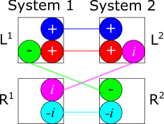
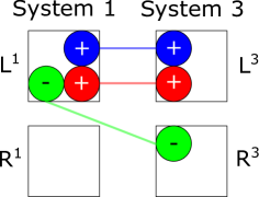
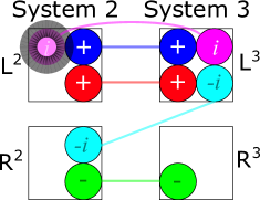
Figure 1: The subpairs and corresponding 2-structures for of the 3-party system. All of the edges of the corresponding 3-structure can be read off of these three diagrams.

Consider three 2-position quantum systems, each with an eigenbasis $(|L\rangle,|R\rangle)$ which are prepared (pre-selected) in the entangled state,

$$|\psi\rangle=\big{(}2|LLL\rangle-|LRR\rangle+i|RLL\rangle-i|RRL\rangle\big{)}/\sqrt{7},$$ (28)

and post-selected in the product state

$$|\varphi\rangle=\big{(}|L\rangle+|R\rangle\big{)}\big{(}|L\rangle+|R\rangle\big{)}\big{(}|L\rangle+|R\rangle\big{)}/\sqrt{8}.$$ (29)

The weak values of the eight rank-1 projector are $|LLL|_{w}=2$, $|LRR|_{w}=-1$, $|RLL|_{w}=i$, $|RRL|_{w}=-i$, and $|LLR|_{w}=|LRL|_{w}=|RLR|_{w}=|RRR|_{w}=0$, which correspond to five (nonzero) 3-structures.

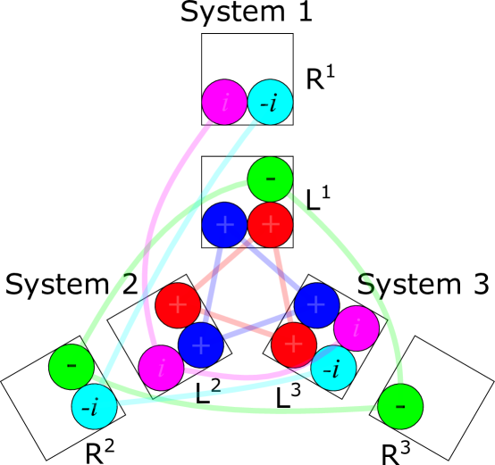
Figure 2: The five 3-structures, each a different color, for the entangled pre-selection $|\psi\rangle=\big{(}2|LLL\rangle-|LRR\rangle+i|RLL\rangle-i|RRL\rangle\big{)}/\sqrt{7}$ and post-selection $|\varphi\rangle=\big{(}|L\rangle+|R\rangle\big{)}\big{(}|L\rangle+|R\rangle\big{)}\big{(}|L\rangle+|R\rangle\big{)}/\sqrt{8}$, and their corresponding counterparticles, with each web assigned a different color. The 2-structures for any 2 subsystems are just the subgraphs of the graphs shown here, which can be verified by considering Fig. 1 - and the 1-structures are just the counterparticles themselves.

To find the edges of these 3-structures we will need to consider the 2-structures corresponding to each pair of fundamental subsystems. Summing over system 3 we find the weak values for the product projectors onto systems 1 and 2,

$$|L^{1}L^{2}|_{w}=|LLL|_{w}+|LLR|_{w}=2,$$ (30)

$$|L^{1}R^{2}|_{w}=|LRL|_{w}+|LRR|_{w}=-1,$$ (31)

$$|R^{1}L^{2}|_{w}=|RLL|_{w}+|RLR|_{w}=i,$$ (32)

$$|R^{1}R^{2}|_{w}=|RRL|_{w}+|RRR|_{w}=-i,$$ (33)

summing over system 2 we find the weak values for the product projectors onto systems 1 and 3,

$$|L^{1}L^{3}|_{w}=|LLL|_{w}+|LRL|_{w}=2,$$ (34)

$$|L^{1}R^{3}|_{w}=|LLR|_{w}+|LRR|_{w}=-1,$$ (35)

$$|R^{1}L^{3}|_{w}=|RLL|_{w}+|RRL|_{w}=0,$$ (36)

$$|R^{1}R^{3}|_{w}=|RLR|_{w}+|RRR|_{w}=0,$$ (37)

and summing over system 1 we find the weak values for the product projectors onto systems 2 and 3,

$$|L^{2}L^{3}|_{w}=|LLL|_{w}+|RLL|_{w}=2+i,$$ (38)

$$|L^{2}R^{3}|_{w}=|LLR|_{w}+|RLR|_{w}=0,$$ (39)

$$|R^{2}L^{3}|_{w}=|LRL|_{w}+|RRL|_{w}=-i,$$ (40)

$$|R^{2}R^{3}|_{w}=|LRR|_{w}+|RRR|_{w}=-1.$$ (41)

The configurations of 2-structures for these subpairs are shown in Fig 1.

The five 3-structures for this PPS are shown in Fig. 2. Note that for this example the three real 3-structures are fully connected, while the two imaginary 3-structures are not.

This example also allows us to consider measurements of lower-rank projectors of an entangled system. To measure an $N$-structure, the pointer must be somehow coupled to the rank-1 projector, which is a product of the values of all $N$ systems at $N$ particular locations, and thus the pointer must somehow interact at all $N$ locations during the PPS interval. In all cases, the end result is that the pointer has received a quasi-classical impulsive shift corresponding to the weak value. For projectors corresponding to $n<N$ systems and locations, the pointer only needs to couple to the $n$ sites, and the shift is determined using the $n$-structure subgraph of the $N$-structure corresponding to those systems. Note that a physical weak measurement inherently disturbs both systems, and so there is always some mixture of the purely impulsive shift due to the counterparticles and higher-order entanglement effects, which are negligible in the weak regime.

III Discussion

III.1 The Counterparticle Representation of All Observables

All of the cases we have examine so far considered a single fine-grained basis for a given PPS, along with various coarse-grainings of that same basis, since this is where the PPS paradoxes originate, but the weak values are defined for every observable of the system, and the counterparticle model should provide a single consistent description of all of these weak values. We show that this can be done by choosing a cardinal set of observables, and rather than a counterparticle being in just one state of the system, it is simultaneously in one eigenstate of each cardinal observable.

For a single cardinal direction $n$, we have a set of distributions of counterparticle configurations $\{C_{ni}\}$, each of which occurs with probability $P_{ni}$. Each $C_{ni}$ is a vector with the same dimension as the Hilbert space of the system, and each component is a complex integer corresponding to a definite set of real and/or imaginary counterparticles. The general distribution is obtained by taking the Cartesian product of all such cardinal sets, multiplying the corresponding probabilities, and the corresponding counterparticle sets. Note that each quasi-classical 2-level particle is in a definite state of all three observables, even though none of them commute. The weak value of just one of the cardinal projectors is obtained by summing over all values of the projectors belonging to other cardinal observables.

It will be useful to introduce a pseudo-density matrix for the PPS which we call the upsidedown state, $\breve{\rho}\equiv|\psi\rangle\langle\varphi|/\langle\varphi|\psi\rangle$, which satisfies $\breve{\rho}^{2}=\breve{\rho}$ and Tr$\breve{\rho}=1$, but is clearly non-Hermitian. The utility of the upsidedown state is that we now have $A_{w}=$Tr$\breve{\rho}A$, in analogy to the usual expectation value $\langle A\rangle=$Tr$\rho A$.

Now, in a 2-level system, the cardinal set is $(\sigma_{x},\sigma_{y},\sigma_{z})$, which we can see by decomposing the upside-down state for a general PPS as,

$$\breve{\rho}\equiv\frac{|\psi\rangle\langle\varphi|}{\langle\varphi|\psi\rangle}=\big{(}I+(\sigma_{x})_{w}\sigma_{x}+(\sigma_{y})_{w}\sigma_{y}+(\sigma_{z})_{w}\sigma_{z}\big{)}/2=(I+\vec{w}\cdot\vec{\sigma})/2,$$ (42)

where $\vec{w}$ is the vector of cardinal weak values. The weak value of an observable $A$ is then,

$$A_{w}=\textrm{Tr}(\breve{\rho}A)=\big{[}\textrm{Tr}(A)+(\sigma_{x})_{w}\textrm{Tr}(\sigma_{x}A)+(\sigma_{y})_{w}\textrm{Tr}(\sigma_{y}A)+(\sigma_{z})_{w}\textrm{Tr}(\sigma_{z}A)\big{]}/2=A_{0}+\vec{w}\cdot\vec{A},$$ (43)

where $\vec{A}$ is the vector of normalized expectation values $A_{x}=\textrm{Tr}(\sigma_{x}A)/2$, $A_{y}=\textrm{Tr}(\sigma_{y}A)/2$, $A_{z}=\textrm{Tr}(\sigma_{z}A)/2$, and $A_{0}=\textrm{Tr}(A)/2$. For the case of a the Pauli observable in the direction of unit vector $\hat{n}$, this reduces to the simple form,

$$(\sigma_{\hat{n}})_{w}=\vec{w}\cdot\hat{n}.$$ (44)

Thus we can obtain the weak values along any direction $\hat{n}$ simply by knowing the cardinal weak values, and we can still use the same set of particles and counterparticles in their combined eigenstates to obtain the weak value in any direction.

Of course, we could rotate the coordinate system and find a new representation in terms of counterparticles for the new cardinal observables. This is yet another symmetry of the counterparticle model, since the descriptions of the same physical system may call for a completely different counterparticle representation in the different coordinate system.

As a simple example, consider a single pigeon from the quantum pigeonhole paradox, with pre-selection $|\psi\rangle=|L\rangle+|R\rangle$ and post-selection $|\varphi\rangle=|L\rangle+i|R\rangle$ for each 2-level system. Recalling that $\sigma_{z}=|L\rangle\langle L|-|R\rangle\langle R|$, we also have $\sigma_{x}|\psi\rangle=|\psi\rangle$, and $\sigma_{y}|\varphi\rangle=|\varphi\rangle$, we can see that the weak vector is $\vec{w}=(1,1,i)$. We thus have upside-down state $\breve{\rho}=(I+\sigma_{x}+\sigma_{y}+i\sigma_{z})/2$. For $x$ and $y$ the simplest configurations both have a single positive particle in $\Pi_{+x}$ and $\Pi_{+y}$ ($C_{x1}=[1,0]$, and $C_{y1}=[1,0]$), respectively, with probability 1. For $z$, the simplest case we can use has, with probability $P_{z1}=1/2$, a single positive particle in $\Pi_{+z}$ ($C_{z1}=[1,0])$, and with probability $P_{z2}=1/2$ there is a positive imaginary particle in $\Pi_{+z}$ and positive real particle plus a negative imaginary particle in $\Pi_{-z}$ ($C_{z2}=[1+i,i]$). The Cartesian product of these three distributions has, with probability $P_{1}=1/2$, a positive counterparticle in joint state $\Pi_{+x,+y,+z}$ ($C_{1}=[1,0,0,0,0,0,0,0,0]$), and with probability $P_{2}=1/2$ a positive imaginary particle in $\Pi_{+x,+y,+z}$ and positive real particle plus a negative imaginary particle in $\Pi_{+x,+y,-z}$ ($C_{2}=[i,1-i,0,0,0,0,0,0,0]$), where the configurations $C_{j}$ now include counterparticles of all eight joint types in canonical order.

To make the situation slightly more interesting, we rotate the coordinate system so that the direction of the post-selection changes from $\hat{y}$ to $(\hat{y}+\hat{z})/\sqrt{2}$ on the Bloch sphere, which is still in the plane perpendicular to the direction of the pre-selection $\hat{x}$. Formally, we have $|\varphi^{\prime}\rangle=\cos(\pi/8)|L\rangle+i\sin(\pi/8)|R\rangle$ and $|\psi^{\prime}\rangle=|\psi\rangle$, which results in the cardinal weak vector $\vec{w}=\big{(}1,(1-i)/\sqrt{2},(1+i)/\sqrt{2}\big{)}$. The same upside down state is now represented as $\breve{\rho}=\Big{(}I+\sigma_{x}+\frac{1-i}{\sqrt{2}}\sigma_{y}+\frac{1+i}{\sqrt{2}}\sigma_{z}\Big{)}/2$ in the new coordinates, from which we obtain $(\Pi^{\pm}_{y})_{w}=(1\pm(1-i)/\sqrt{2})$ and $(\Pi^{\pm}_{z})_{w}=(1\pm(1+i)/\sqrt{2})$.

As before we have $\Pi_{+x}$ with probability 1, but for the $y$ direction we now have $P_{y1}=\frac{1}{2\sqrt{2}}$, $P_{y2}=\frac{1}{2}$, and $P_{y3}=\frac{1}{2}-\frac{1}{2\sqrt{2}}$, with corresponding configurations $C_{y1}=[1-i,i]$, $C_{y2}=[1,0]$, and $C_{y3}=[0,1]$, and for the $z$ direction we have $P_{z1}=\frac{1}{2\sqrt{2}}$, $P_{z2}=\frac{1}{2}$, and $P_{z3}=\frac{1}{2}-\frac{1}{2\sqrt{2}}$, with corresponding configurations $C_{z1}=[1+i,-i]$, $C_{z2}=[1,0]$, and $C_{z3}=[0,1]$.

The joint distribution then has nine configurations, each with a probability and a set of counterparticles obtained by taking the products of the three individual sets. For example, the probability to obtain the first configuration is $P_{1}=(1)(\frac{1}{2\sqrt{2}})(\frac{1}{2\sqrt{2}})=\frac{1}{8}$, and the set of counterparticles in the joint state $\Pi_{+x,+y,+z}$ in that configuration is $(1)(1-i)(1+i)=2$. The full set of probabilities and configurations is given in Fig. 3

Figure 3: The probabilities and simplified counterparticle representation of the PPS with upside-down state $\breve{\rho}=\Big{(}I+\sigma_{x}+\frac{1-i}{\sqrt{2}}\sigma_{y}+\frac{1+i}{\sqrt{2}}\sigma_{z}\Big{)}/2$. The marginal weak value of $\Pi^{\pm}_{i}$ is given by summing over the corresponding columns.

$P$	$(\Pi_{x}^{+},\Pi_{y}^{+},\Pi_{z}^{+})$	$(\Pi_{x}^{+},\Pi_{y}^{+},\Pi_{z}^{-})$	$(\Pi_{x}^{+},\Pi_{y}^{-},\Pi_{z}^{+})$	$(\Pi_{x}^{+},\Pi_{y}^{-},\Pi_{z}^{-})$	$(\Pi_{x}^{-},\Pi_{y}^{+},\Pi_{z}^{+})$	$(\Pi_{x}^{-},\Pi_{y}^{+},\Pi_{z}^{-})$	$(\Pi_{x}^{-},\Pi_{y}^{-},\Pi_{z}^{+})$	$(\Pi_{x}^{-},\Pi_{y}^{-},\Pi_{z}^{-})$
$\frac{1}{8}$	$2$	$-1-i$	$-1+i$	$1$	$0$	$0$	$0$	$0$
$\frac{1}{4\sqrt{2}}$	$1-i$	$0$	$i$	$0$	$0$	$0$	$0$	$0$
$\frac{1}{4\sqrt{2}}-\frac{1}{8}$	$0$	$1-i$	$0$	$i$	$0$	$0$	$0$	$0$
$\frac{1}{4\sqrt{2}}$	$1+i$	$-i$	$0$	$0$	$0$	$0$	$0$	$0$
$\frac{1}{4}$	$1$	$0$	$0$	$0$	$0$	$0$	$0$	$0$
$\frac{1}{4}-\frac{1}{4\sqrt{2}}$	$0$	$1$	$0$	$0$	$0$	$0$	$0$	$0$
$\frac{1}{4\sqrt{2}}-\frac{1}{8}$	$0$	$0$	$1+i$	$-i$	$0$	$0$	$0$	$0$
$\frac{1}{4}-\frac{1}{4\sqrt{2}}$	$0$	$0$	$1$	$0$	$0$	$0$	$0$	$0$
$\frac{3}{8}-\frac{1}{2\sqrt{2}}$	$0$	$0$	$0$	$1$	$0$	$0$	$0$	$0$

Now, when the 2-level system is the spin of a particle, it is straighforward to imagine a single particle which somehow simultaneously has the three properties $\sigma_{x}=\sigma_{y}=\sigma_{z}=+1$, but if the system is a spatial superposition, then the interpretation is more subtle. If the $\Pi^{\pm}_{z}$ are orthogonal spatial states, like the arms of an MZ, then $\Pi^{\pm}_{x}$ and $\Pi^{\pm}_{y}$ are spatial superpositions, so how can a particle with a single trajectory be in a simultaneous state of all three? The simplest answer seems to be that the spatial basis is the one that tells us where the particle is actually located, since each projectors can be measured at only one location. The other states are internal properties of the particle, which are only revealed by a measurement which couples to the system at both locations (measurements of say $\sigma_{x}$ or $\sigma_{y}$), similar to measuring $N$-structures.

Finally, this type of cardinal representation can be found in all dimensions by expanding the upside-down state into the set of $d$-dimensional generalized Gell-Mann matrices. This works just as in the $d=2$ case above, because the Gell-Mann matrices are all traceless, as is the product of any two of them, and the trace of their squares are always 2. There are $d^{2}-1$ different Hermitian Gell-Mann matrices, which combined with the identity span the space of all observables of the system (with real coefficients, and the space of all operators with complex coefficients). This means the general expanded form of the upside-down state is,

$$\breve{\rho}=\frac{1}{d}I+\frac{1}{2}\sum_{i=1}^{d^{2}-1}(g_{i})_{w}g_{i}=\frac{1}{d}I+\frac{1}{2}\vec{w}_{d}\cdot\vec{g},$$ (45)

and thus a complete counterparticle representation can always be constructed in this way, with $\vec{g}$ a vector of the $d^{2}-1$ generalized Gell-Mann matrices, and $\vec{w}_{d}$ the vector of their weak values. Likewise a general observable can be said to point in a particular direction $\hat{n}_{d}$ in the $(d^{2}-1)$-dimensional real space of cardinal matrices, and we can expand a general Gell-Mann observable as $g_{\hat{n}_{d}}=\hat{n}_{d}\cdot\vec{g}$, and we again obtain,

$$(g_{\hat{n}_{d}})_{w}=\vec{w}_{d}\cdot\hat{n}_{d},$$ (46)

which shows that this cardinal counterparticle representation defines the weak values of all observables of the system.

Finally for dimensions $d=2^{N}$, a similar expansion can be constructed using the observables of the $N$-qubit Pauli group, which are all tensor products, and so this representation may be more convenient for some applications.

III.2 Intermediate Interaction Strength

The counterparticle model is a good physical approximation only in the limit of weak measurements. The weak limit is the first order approximation for small $d/\varepsilon$. We expect that a more elaborate model can be devised in which higher order terms also have a physical interpretation, and become increasingly relevant as the interaction strength increases. In the projective measurement limit, this would require interpreting an infinite number of terms, and more importantly, this is the limit where the interaction induces a post-selection, and so as the interaction strength is slowly increased from zero, at first there may be higher order objects in the counterparticle model (we have not yet explored this), but then this entire picture starts to give way, to be replaced by a new collapse event. This raises a more fundamental questions about the range of physical situations this model can describe.

In particular, consider a system that undergoes frequent periodic measurement interactions, each of small, but not insignificant strength. This system is unlikely to collapse due to any one measurement, and instead its continuous weak measurement readout will wander back and forth, only eventually collapsing to an eigenvalue after many measurements garcia2017past . Then it will tend to remain there for a little while due to an effect called Zeno pinning, but eventually its Hamiltonian dynamics will set it back to wandering, and then to another random collapse.

Now, consider a long period of wandering during which the system never actually collapses to either eigenvalue, which can be more readily accomplished by alternating kicks in complementary measurement bases garcia2016probing . It has been shown in numerical simulations that due to the random kicks, the state of a system rapidly becomes independent of its previous states, even if it never fully collapses. The simulations also show that the continuous weak measurement readout likewise becomes rapidly independent of the future states of the system. This means that the intermediate (nearly weak) values that are being continuously read out simply do not have a projective pre-selection or a projective post-selection. Instead, the pre- and post-selection occurred gradually, over the course of enough random kicks to screen a small time interval off from both its past and future. To give a rough idea of how this could work, suppose that the measurement events are indexed by $i$, and the state is screen off after $n$ such events. Then the physical readout at event $i$ will be centered on roughly the weak value, using the some function of the physical states at events $i-1$, $i-2$,…, $i-n$, as the pre-selection, and some function of $i+1$, $i+2$,…, $i+n$ as the post-selection. The trouble with this is that we cannot actually know the physical state at each event, as we do in the case of projective measurements, and this seems to be the price we pay for the counterparticle model to apply to physical situations like this. Nevertheless, nature knows the PPS, even when it cannot be experimentally observed.

References

- (1) Aharonov Y, Cohen E, Landau A, Elitzur AC (2017) The case of the disappearing (and re-appearing) particle. Scientific reports 7(1):531.
- (2) Aharonov Y, Popescu S, Rohrlich D, Skrzypczyk P (2013) Quantum cheshire cats. New Journal of Physics 15(11):113015.
- (3) Denkmayr T, et al. (2014) Observation of a quantum cheshire cat in a matter-wave interferometer experiment. Nature communications 5:4492.
- (4) Aharonov Y, Cohen E, Popescu S (2015) A current of the cheshire cat’s smile: Dynamical analysis of weak values. arXiv preprint arXiv:1510.03087.
- (5) Aharonov Y, et al. (2016) Quantum violation of the pigeonhole principle and the nature of quantum correlations. PNAS 113(3):532–535.
- (6) Waegell M, Tollaksen J (2018) Contextuality, pigeonholes, cheshire cats, mean kings, and weak values. Quantum Studies: Mathematics and Foundations 5(2):325–349.
- (7) Waegell M, et al. (2017) Confined contextuality in neutron interferometry: Observing the quantum pigeonhole effect. Physical Review A 96(5):052131.
- (8) Aharonov Y, Cohen E, Tollaksen J (2018) Completely top–down hierarchical structure in quantum mechanics. Proceedings of the National Academy of Sciences 115(46):11730–11735.
- (9) Elouard C, Waegell M, Huard B, Jordan AN (2019) Spooky work at a distance: an interaction-free quantum measurement-driven engine. arXiv preprint arXiv:1904.09289.
- (10) Waegell M, Elouard C, Jordan AN (2020) Energy-based weak measurement. Quantum Studies: Mathematics and Foundations pp. 1–6.
- (11) Elitzur AC, Vaidman L (1993) Quantum mechanical interaction-free measurements. Foundations of Physics 23(7):987–997.
- (12) García-Pintos LP, Dressel J (2017) Past observable dynamics of a continuously monitored qubit. Physical Review A 96(6):062110.
- (13) García-Pintos LP, Dressel J (2016) Probing quantumness with joint continuous measurements of noncommuting qubit observables. Physical Review A 94(6):062119.