Non-Hermitian Absorption Spectroscopy

Abstract

While non-Hermitian Hamiltonians have been experimentally realized in cold atom systems, it remains an outstanding open question of how to experimentally measure their complex energy spectra in momentum space for a realistic system with boundaries. The existence of non-Hermitian skin effects may make the question even more difficult to address given the fact that energy spectra for a system with open boundaries are dramatically different from those in momentum space; the fact may even lead to the notion that momentum-space band structures are not experimentally accessible for a system with open boundaries. Here, we generalize the widely used radio-frequency spectroscopy to measure both real and imaginary parts of complex energy spectra of a non-Hermitian quantum system for either bosonic or fermionic atoms. By weakly coupling the energy levels of a non-Hermitian system to auxiliary energy levels, we theoretically derive a formula showing that the decay of atoms on the auxiliary energy levels reflects the real and imaginary parts of energy spectra in momentum space. We further prove that measurement outcomes are independent of boundary conditions in the thermodynamic limit, providing strong evidence that the energy spectrum in momentum space is experimentally measurable. We finally apply our non-Hermitian absorption spectroscopy protocol to the Hatano-Nelson model and non-Hermitian Weyl semimetals to demonstrate its feasibility.

Measurements based on spectroscopy providing band structure information play a key role in identifying various topological phases in condensed matter and cold atom systems Torma2016Review ; Ding2019NRP ; Takagi2020JCMP ; NHLinearResponse ; Shen2021RMP ; Zwierlein2021NP . In the past few years, non-Hermitian topological physics has seen a rapid advance ChristodoulidesNPReview ; XuReview ; ZhuReview ; UedaReview ; BergholtzReview . Such systems usually exhibit complex band structures with exceptional points or rings Zhen2015nat ; Xu2017PRL ; Nori2017PRL ; Kozii2017 ; Zyuzin2018PRB ; Zhou2018 ; Cerjan2018PRB ; Yoshida2018PRB ; Zhao2018PRB ; Carlstrom2018PRA ; HuPRB2019 ; Wang2019PRB ; Yoshida2019PRB ; Ozdemir2019 ; Cerjan2019nat ; Kawabata2019PRL ; Zhang2019PRL ; Zhang2020PRL ; Chuanwei2020PRL ; Yang2020PRL ; Wang2021PRL ; Nagai2020PRL ; Nori2021PRL ; Yuliang2021 ; An2022PRB . In cold atom systems, non-Hermitian Hamiltonians have been experimentally realized by introducing atom loss LuoNC2018 ; JoarXiv2021 ; Gadway2019NJP ; Yan2020PRL ; Takahashi2020PTEP ; Esslinger2021arxiv ; Esslinger2021PRX . The parity-time ($\mathcal{PT}$) symmetry breaking has been observed by measuring the population of an evolving state of a system through quench dynamics LuoNC2018 ; JoarXiv2021 ; WeiZhang2021PRL . However, such a method is very hard to generalize to a generic case without $\mathcal{PT}$ symmetry. In fact, while there are practical proposals on how to realize non-Hermitian topological phases in cold atom systems Xu2017PRL ; Yang2021 ; Cui2021 ; Lang2022 , such as non-Hermitian Weyl semimetals, it remains an outstanding open question of how to experimentally measure both the real and imaginary parts of energy spectra in a non-Hermitian cold atom system. Moreover, one of the most important phenomena in non-Hermitian systems is the non-Hermitian skin effects (NHSEs); with such effects, band structures under open boundary conditions (OBCs) are dramatically different from those under periodic boundary conditions (PBCs) Yao2018PRL1 ; TonyLee ; Xiong2018JPC ; Torres2018PRB ; Kunst2018PRL ; Qibo2020 ; Lang2019PRB ; Okuma2020PRL ; Slager2020PRL ; ChenFang2020PRL . The difference naturally leads to a question of whether the existence of NHSEs makes it impossible to measure the energy spectra in momentum space for a system with open boundaries. The question is important in light of the fact that most experiments are performed in a geometry with boundaries.

Figure 1: (a) Schematics of non-Hermitian absorption spectroscopy where a non-Hermitian system is coupled to auxiliary energy levels by a microwave field or a laser beam. Atoms are initially prepared on the auxiliary levels, and their occupancy on the auxiliary levels is finally measured after a period of time. (b) A typical example of the measured occupancy as a function of the detuning $\delta$ with an occupancy dip at $\delta=\delta_{0}$. The center and the width of the dip are related to the real and the imaginary part of an eigenenergy of a non-Hermitian system, respectively.

A widely used spectroscopy in cold atom systems is the radio-frequency (RF) spectroscopy Torma2016Review ; Zwierlein2021NP . There, auxiliary energy levels are weakly coupled to system energy levels so that atoms will either be driven from occupied auxiliary levels to empty system levels or from occupied system levels to empty auxiliary levels, when the frequency of radio waves or microwaves match the energy difference. By imaging the transmitted atoms, such a spectroscopy allows us to map out the energy band dispersion, similar to angle resolved photoemission spectroscopy (ARPES) in solid-state materials. In the paper, we generalize the RF spectroscopy to a non-Hermitian system to allow for measurements of both the real and imaginary parts of a complex energy spectrum in cold atom systems (see Fig. 1). For a non-Hermitian system in cold atoms, there always exists a total loss of atoms on the system levels, making it impossible to image any atoms on the system levels after a long period of time. We thus consider initial preparations of atoms on the auxiliary levels followed by measurements of atoms on these levels instead of system levels. Using linear response theory, we derive a formula describing the population of auxiliary levels, based on which one can extract not only real parts of the system’s band structure in momentum space but also its imaginary parts. We further prove that measurement results are independent of boundary conditions in the thermodynamic limit despite the existence of NHSEs; this is in stark contrast to the results in Ref. Sato2021PRL showing that ARPES might be sensitive to skin effects. Finally, we utilize the Hatano-Nelson (HN) model and a non-Hermitian Weyl semimetal to demonstrate the feasibility of the spectroscopy.

Momentum-resolved non-Hermitian Absorption spectroscopy.—We start by considering a generic translation-invariant non-Hermitian system described by a Hamiltonian $\hat{\mathcal{H}}_{\text{s}}=\sum_{i\alpha,j\beta}[H_{\text{s}}]_{i\alpha,j\beta}\hat{c}_{i\alpha}^{\dagger}\hat{c}_{j\beta}$ with $\hat{c}_{i\alpha}^{\dagger}$ ($\hat{c}_{i\alpha}$) being either the fermionic or bosonic creation (annihilation) operator acting on the $\alpha$th degree of freedom of the $i$th unit cell. We assume that the non-Hermitian Hamiltonian $\hat{\mathcal{H}}_{\text{s}}$ is purely dissipative, i.e. $\text{Im}(\lambda)<0$ for any eigenvalue $\lambda$ of $H_{\text{s}}$. To measure the system’s complex energy spectra, we couple the first degree of freedom of each unit cell to an auxiliary energy level by a microwave field such that the full Hamiltonian under rotating wave approximations becomes ($\hbar=1$)

$$\hat{\mathcal{H}}=\hat{\mathcal{H}}_{\text{s}}+\hat{\mathcal{H}}_{\text{a}}+({\Omega}/{2})\sum\nolimits_{j}(\hat{c}_{j1}^{\dagger}\hat{a}_{j}+\hat{a}_{j}^{\dagger}\hat{c}_{j1})$$ (1)

with $\hat{\mathcal{H}}_{\text{a}}=\sum_{j}\big{[}J(\hat{a}_{j}^{\dagger}\hat{a}_{j+1}+\hat{a}_{j+1}^{\dagger}\hat{a}_{j})-(\omega-\omega_{\text{a}})\hat{a}_{j}^{\dagger}\hat{a}_{j}\big{]}$ describing the auxiliary levels, where $\hat{a}_{j}^{\dagger}$ ($\hat{a}_{j}$) is the creation (annihilation) operator acting on the $j$th auxiliary level, $J$ is the hopping strength between nearest-neighbor auxiliary levels, $\omega_{\text{a}}$ is the energy of the auxiliary level of an atom measured relative to the first system energy level of the atom, and $\omega$ is the frequency of the microwave field ($\delta=\omega-\omega_{\text{a}}$ is the detuning). The final term depicts the coupling between system and auxiliary levels with $\Omega$ being the Rabi frequency of the microwave field. Note that $J$, $\omega$, $\omega_{a}$ and $\Omega$ are all real numbers.

To measure the energy spectrum of the system, we first prepare a cloud of fermionic atoms on the first band of auxiliary levels described by the many-body state $|\psi_{0}^{(M)}\rangle=\prod_{k}\hat{a}_{k}^{\dagger}|0\rangle$ with $|0\rangle$ being the vacuum state at a low temperature. For bosonic atoms, we consider a finite temperature ensemble (see Supplemental Material S-1 B for detailed discussions). We then switch on the coupling between system and auxiliary levels by shining a microwave field on the atoms. After a long period of time, we perform the time-of-flight measurement to obtain the atom population on the auxiliary levels at each momentum $k$. While the dynamics of a dissipative cold atom system is usually described by the master equation, in Supplemental Material S-1, we have proved that the atom number on auxiliary levels at momentum $k$ is given by $N_{\text{a},k}=\text{Tr}[\rho(t)\hat{a}_{k}^{\dagger}\hat{a}_{k}]=N_{\text{0},k}\langle 0|\hat{a}_{k}e^{\text{i}\hat{\mathcal{H}}^{\dagger}t}\hat{a}_{k}^{\dagger}\hat{a}_{k}e^{-\text{i}\hat{\mathcal{H}}t}\hat{a}_{k}^{\dagger}|0\rangle$, where $N_{\text{0},k}=\text{Tr}[\rho(0)\hat{a}_{k}^{\dagger}\hat{a}_{k}]$. Here $\rho(t)$ is the density matrix evolving from either the initial state $\rho(0)=|\psi_{0}^{(M)}\rangle\langle\psi_{0}^{(M)}|$ for fermions ($N_{\text{0},k}=1$ in this case) or a finite temperature ensemble for bosons. The result indicates that the dynamics is completely determined by the non-Hermitian Hamiltonian $\hat{\mathcal{H}}$. This allows us to use a single-particle state $|\psi_{\text{a}}^{k}\rangle=\hat{a}_{k}^{\dagger}|0\rangle$ ($|\psi_{\text{a}}^{k}\rangle$ is an eigenstate of $\hat{\mathcal{H}}_{\text{a}}$ with eigenenergy $E_{k}=-\delta+2J\cos k$) on auxiliary levels as an initial state to derive the protocol.

With an initial state prepared as $|\psi_{\text{a}}^{k}\rangle$ on auxiliary levels, we use the linear response theory TormaBook to derive the population of auxiliary levels at time $t$ under PBCs as Supplementary

$$N_{\text{a}}(t)=N_{\text{a}}(0)\exp(-\kappa t)$$ (2)

with $\kappa=-\frac{\Omega^{2}}{2}\sum_{m}\frac{a_{km}^{(1)}\gamma_{km}-b_{km}^{(1)}\Delta_{km}}{\Delta_{km}^{2}+\gamma_{km}^{2}}$ and $N_{\text{a}}(0)$ being the initial occupancy of the single-particle state of the auxiliary levels at momentum $k$. The result holds for both bosons and fermions. For simplicity, we will consider $N_{\text{a}}(0)=1$ henceforth. Here, $\Delta_{km}=E_{k}-\varepsilon_{km}$ with $\varepsilon_{km}$ ($-\gamma_{km}$) denoting the real (imaginary) part of eigenenergies of ${\mathcal{H}}_{\text{s}}$, which are labeled by the momentum $k$ and the band index $m$; $a_{km}^{(1)}=\mathrm{Re}[c_{km}^{(1)}]$ and $b_{km}^{(1)}=\mathrm{Im}[c_{km}^{(1)}]$ where $c_{km}^{(\alpha)}=\langle\psi_{\text{s}}^{k\alpha}|u_{\text{R}}^{km}\rangle\langle u_{\text{L}}^{km}|\psi_{\text{s}}^{k\alpha}\rangle$ with $|\psi_{\text{s}}^{k\alpha}\rangle=\hat{c}_{k\alpha}^{\dagger}|0\rangle=\frac{1}{\sqrt{N}}\sum_{j}e^{\text{i}kj}\hat{c}_{j\alpha}^{\dagger}|0\rangle$, $|u_{\text{R}}^{km}\rangle$ being the right eigenstate of the system Hamiltonian, i.e., $\hat{\mathcal{H}}_{\text{s}}|u_{\text{R}}^{km}\rangle=(\varepsilon_{km}-\text{i}\gamma_{km})|u_{\text{R}}^{km}\rangle$, and $\langle u_{\text{L}}^{km}|$ being the corresponding left one. In the derivation, we have assumed that $\Omega$ is sufficiently small compared with the decay rates of system states and $t\gg 1/\gamma_{km}$. One can also see the similarity between $-4\ln[N_{\text{a}}(t)]/(\Omega^{2}t)$ given by Eq. (2) and the ${\mathcal{H}}_{\text{s}}$’s spectral function, $A(k,\omega)=-2\text{Im}\,\text{Tr}[(\omega-{\mathcal{H}}_{\text{s}})^{-1}]=\sum_{m}{2\gamma_{km}}/{[(\omega-\varepsilon_{km})^{2}+\gamma_{km}^{2}]}$ given the fact that $\sum_{\alpha}c_{km}^{(\alpha)}=1$.

We now briefly summarize the derivation of Eq. (2) (the details can be found in Supplemental Material S-2). We first write the full Hamiltonian (1) as $\hat{\mathcal{H}}=\hat{\mathcal{H}}_{\text{0}}+\hat{\mathcal{V}}$ with $\hat{\mathcal{H}}_{\text{0}}=\hat{\mathcal{H}}_{\text{s}}+\hat{\mathcal{H}}_{\text{a}}$. In the interaction picture, the state at time $t$ is given by $|\psi^{I}(t)\rangle=\hat{U}^{I}(t,0)|\psi_{\text{a}}^{k}\rangle$ where $\hat{U}^{I}(t,t_{0})=1-\text{i}\int_{t_{0}}^{t}dt^{\prime}\hat{\mathcal{V}}^{I}(t^{\prime})+\mathcal{O}(\Omega^{2})$ is the time evolution operator. Through careful derivations, we find that $\dot{N}_{\text{a}}(t)=\langle\psi^{I}(t)|\hat{\dot{N}}_{\text{a}}^{I}(t)|\psi^{I}(t)\rangle=-\kappa$. Considering the fact that $N_{\text{a}}(t)$ decreases with time, we obtain $\dot{N}_{\text{a}}(t)=-\kappa N_{\text{a}}(t)$, which yields Eq. (2) after integration. The result has also been numerically confirmed. We note that different from Refs. NHLinearResponse ; Zhai2021PRL where a non-Hermitian perturbation is added in a Hermitian system, we here include a Hermitian perturbation to measure a non-Hermitian system’s properties.

Based on Eq. (2), we see that the spectral line of $-\ln[N_{\text{a}}(t)]$ as a function of $-\delta$ consists of multiple peaks centered at $-\delta=\varepsilon_{km}-2J\cos k$ with half widths approximated by $2\gamma_{km}$. In fact, Eq. (2) allows us to obtain both $\varepsilon_{km}$ and $\gamma_{km}$ (as well as the quantities $a_{km}$ and $b_{km}$) by fitting the spectral line using this formula.

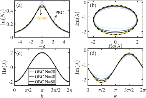
Figure 2: (a) The spectral lines of the HN model at $k=\pi/2$ with the yellow line obtained from Eq. (4) and the dashed black and solid blue lines numerically computed for a system under PBCs and OBCs, respectively. Energy spectra in the complex energy plane (b), real (c) and imaginary parts (d) of energies with respect to $k$, where $k$ denotes the Bloch momentum as we consider a Bloch state as an initial state. The energies are extracted by fitting the numerically calculated spectral lines under PBCs (dashed black lines) and OBCs (solid blue lines) based on Eq. (4) in comparison with the theoretical result, $\varepsilon_{k}=2J_{s}\cos k+2\text{i}g\sin k-2\text{i}\gamma$ (the yellow lines). Here, $J_{s}=-1$, $J=-0.02$, $g=-0.5$, $\gamma=0.6$, $\Omega=0.1$ and $t=200$.

Before applying our method to several paradigmatic models, we wish to prove that our conclusion is independent of boundary conditions in the thermodynamic limit, although we derive the results under PBCs. Here we briefly summarize the proof; the detailed one can be found in Supplemental Material S-3. We first prove that $D=\langle k\alpha|e^{-\text{i}\hat{\mathcal{H}}_{\text{o}}t}-e^{-\text{i}\hat{\mathcal{H}}_{\text{p}}t}|k^{\prime}\alpha^{\prime}\rangle\propto 1/N$ where $|k\alpha\rangle$ is the k-space basis vector, and letters ‘o’ (‘p’) are used to denote quantities under OBCs (PBCs). Assuming the hopping range is finite, we obtain $\langle k\alpha|\hat{B}|k^{\prime}\alpha^{\prime}\rangle=f_{\alpha\alpha^{\prime}}(k,k^{\prime})/N$ where $\hat{B}=\hat{\mathcal{H}}_{\text{p}}-\hat{\mathcal{H}}_{\text{o}}$ and $f_{\alpha\alpha^{\prime}}(k,k^{\prime})$ is independent of $N$. We then prove that each term in $D_{n}=\langle k\alpha|(\hat{\mathcal{H}}_{\text{p}}-\hat{B})^{n}-(\hat{\mathcal{H}}_{\text{p}})^{n}|k^{\prime}\alpha^{\prime}\rangle$ is proportional to $1/N$ and thus conclude that $D=\sum_{n=1}^{\infty}\frac{(-\text{i}t)^{n}}{n!}D_{n}\propto 1/N$. Since $\dot{N}_{\text{a}}^{\text{b}}(t)=(\Omega^{2}/4)\int_{0}^{t}dt^{\prime}\Gamma^{\text{b}}(t,t^{\prime})+\text{H.c.}$ and $\Gamma^{\text{b}}(t,t^{\prime})=-\sum_{q\tilde{q}}\langle\psi_{\text{a}}^{k}|e^{\text{i}\hat{\mathcal{H}}_{\text{a}}^{\text{b}}t}|\psi_{\text{a}}^{q}\rangle\langle\psi_{\text{s}}^{q1}|e^{-\text{i}\hat{\mathcal{H}}_{\text{s}}^{\text{b}}(t-t^{\prime})}|\psi_{\text{s}}^{\tilde{q}1}\rangle\langle\psi_{\text{a}}^{\tilde{q}}|e^{-\text{i}\hat{\mathcal{H}}_{\text{a}}^{\text{b}}t^{\prime}}|\psi_{\text{a}}^{k}\rangle$ ($\text{b}=\text{o},\text{p}$), we derive that $(\Gamma^{\text{o}}-\Gamma^{\text{p}})(t,t^{\prime})\propto 1/N$, yielding $\dot{N}_{\text{a}}^{\text{o}}(t)-\dot{N}_{\text{a}}^{\text{p}}(t)\propto 1/N$. Taking the infinite size limit, we obtain $N_{\text{a}}^{\text{o}}(t)=N_{\text{a}}^{\text{p}}(t)$, implying that the result is independent of boundary conditions in the thermodynamic limit.

Hatano-Nelson model.—To demonstrate the feasibility of our spectroscopy protocol, we apply it to the HN model HN1996PRL (the simplest model that supports NHSEs):

$$\hat{\mathcal{H}}_{\text{s}}^{\text{HN}}=\sum\nolimits_{j}[(J_{s}+g)\hat{c}_{j}^{\dagger}\hat{c}_{j+1}+(J_{s}-g)\hat{c}_{j+1}^{\dagger}\hat{c}_{j}-2\text{i}\gamma\hat{c}_{j}^{\dagger}\hat{c}_{j}],$$ (3)

where $J_{s}$ and $g$ are real parameters describing the hopping strength between nearest-neighbor sites. When $g\neq 0$, the NHSE occurs due to the asymmetric hopping. Here we add an onsite dissipation term $-2\text{i}\gamma\sum_{j}\hat{c}_{j}^{\dagger}\hat{c}_{j}$ with $\gamma>|g|$ to ensure that $\hat{\mathcal{H}}_{\text{s}}^{\text{HN}}$ is purely dissipative. The full Hamiltonian with each system site coupled to an auxiliary level is given by $\hat{\mathcal{H}}^{\text{HN}}=\hat{\mathcal{H}}_{\text{s}}^{\text{HN}}+\sum_{j}[J(\hat{a}_{j}^{\dagger}\hat{a}_{j+1}+\hat{a}_{j+1}^{\dagger}\hat{a}_{j})-\delta\hat{a}_{j}^{\dagger}\hat{a}_{j}+({\Omega}/{2})(\hat{c}_{j}^{\dagger}\hat{a}_{j}+\hat{a}_{j}^{\dagger}\hat{c}_{j})]$. Since $|u_{\text{R}}^{k}\rangle=|u_{\text{L}}^{k}\rangle=|\psi_{\text{s}}^{k}\rangle$ for the HN model, we obtain $a_{k}=1$, $b_{k}=0$ and thus

$$-\ln[N_{\text{a}}(t)]=\frac{\Omega^{2}t}{2}\frac{\gamma_{k}}{(-\delta+2J\cos k-\varepsilon_{k})^{2}+\gamma_{k}^{2}},$$ (4)

which is exactly the spectral function $A(k,\omega)$ up to a constant factor.

To verify our theory, we numerically calculate $N_{\text{a}}(t)$ with respect to $\delta$ and find that the results under PBCs agree very well with Eq. (4) [see Fig. 2(a)]. For open boundaries, while the numerical results slightly deviate from the theoretical ones, the deviation becomes smaller as the system size increases, which is in agreement with our proof that $N_{\text{a}}(t)$ under OBCs approaches the result under PBCs as we increase the system size even when the system exhibits NHSEs.

With each $N_{\text{a}}(t)$ as a function of $\delta$, one can extract the energy information by fitting the function based on Eq. (4). Figure 2(b-d) illustrates the extracted energy spectra under PBCs and OBCs in comparison with the momentum space energy spectra of the system Hamiltonian $\hat{\mathcal{H}}_{\text{s}}^{\text{HN}}$. We see that the results under PBCs agree perfectly well with the system’s complex energy spectra. For open boundaries, while the extracted energy spectra are slightly different from the theoretical results, the discrepancy becomes smaller as the system size becomes larger. We thus conclude that non-Hermitian absorption spectroscopy allows us to extract both real and imaginary parts of complex energy spectra of a non-Hermitian system in momentum space even when the non-Hermitian system has open boundaries and NHSEs.

To further confirm that the spectroscopy measures the energy spectra in momentum space, we study the non-Hermitian Rice-Mele model NHRM2020PRL with NHSEs induced by onsite dissipations in Supplemental Material S-4, which is more relevant to cold atom experiments (also see the proposals in Refs. Yang2021 ; Cui2021 ). We show that the boundary effects can always be significantly reduced by increasing system sizes.

Non-Hermitian Weyl semimetal.—Next, we study a three-dimensional Weyl semimetal with onsite dissipations Xu2017PRL :

$$\hat{\mathcal{H}}_{\text{s}}^{\text{NHWS}}=\sum\nolimits_{\bm{k}}\hat{c}_{\bm{k}}^{\dagger}h_{\bm{k}}\hat{c}_{\bm{k}},$$ (5)

where $\hat{c}_{\bm{k}}^{\dagger}=(\hat{c}_{{\bm{k}}\uparrow}^{\dagger}\ \,\hat{c}_{{\bm{k}}\downarrow}^{\dagger})$ and $h_{\bm{k}}=2t_{\text{SO}}(\sin k_{x}\sigma_{x}+\sin k_{y}\sigma_{y})+[m_{z}-2t_{z}\cos k_{z}-2t_{1}(\cos k_{x}+\cos k_{y})]\sigma_{z}+\text{i}\gamma(\sigma_{z}-\sigma_{0})$ with $t_{\text{SO}}$, $t_{z}$, $t_{1}$ and $m_{z}$ being real system parameters, $\gamma$ depicting the atom loss rate on a hyperfine level Xu2017PRL , and $\{\sigma_{\nu}\}$ ($\nu=x,y,z$) being a set of Pauli matrices. Without onsite dissipations ($\gamma=0$), this model Yong2016PRA ; Yong2019PRB ; Liu2020SB has been experimentally realized in cold atom systems 3DWeylband2021Science . When $\gamma>0$, each Weyl point develops into a Weyl exceptional ring consisting of exceptional points on which $h_{\bm{k}}$ is nondiagonalizable Xu2017PRL . For example, the Weyl point at $(k_{x},k_{y},k_{z})=\{0,0,\arccos[({m_{z}-4t_{1}})/({2t_{z}})]\}$ deforms into a Weyl exceptional ring which can be approximated by $k_{x}^{2}+k_{y}^{2}={\gamma^{2}}/({4t_{\text{SO}}^{2}})$ and $k_{z}=\arccos[({m_{z}-4t_{1}})/({2t_{z}})+{t_{1}\gamma^{2}}/({8t_{z}t_{\text{SO}}^{2}})]$ when $\gamma\ll 2t_{\text{SO}}$.

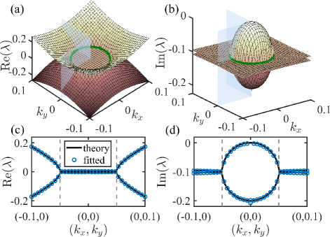
Figure 3: Real (a) and imaginary parts (b) of the extracted eigenenergy of $\hat{\mathcal{H}}_{\text{s}}^{\text{NHWS}}$ in the $(k_{x},k_{y})$ plane obtained by fitting the numerically simulated spectral lines based on Eq. (2). The Weyl exceptional ring is highlighted as a green circle. (c),(d) The sectional view (blue circles) of the fitted energy spectra on the blue planes in (a) and (b), respectively. The black lines refer to the eigenenergies of $h_{\bm{k}}$. The locations of exceptional points are marked out by vertical dashed lines. Without loss of generality, we here set $J=0$ in light of the fact that nonzero $J$ only causes a shift of the spectral line by $2J\sum_{i=x,y,z}\cos k_{i}$. Here, $t_{1}=t_{z}=t_{\text{SO}}=1$, $m_{z}=4$, $\gamma=0.1$ and $k_{z}=\arccos({1}/{800})$.

To measure the Weyl exceptional ring, we couple the spin down degree of freedom of each atom to an auxiliary level. Since the measurement protocol is independent of boundary conditions, we consider the Hamiltonian under PBCs, which reads $\hat{\mathcal{H}}^{\text{NHWS}}=\sum_{\bm{k}}\hat{c}_{\bm{k}}^{\dagger}h_{\bm{k}}\hat{c}_{\bm{k}}+({\Omega}/{2})(\hat{c}_{{\bm{k}}\downarrow}^{\dagger}\hat{a}_{\bm{k}}+\hat{a}_{\bm{k}}^{\dagger}\hat{c}_{{\bm{k}}\downarrow})-\delta\hat{a}_{\bm{k}}^{\dagger}\hat{a}_{\bm{k}}.$ For each initial state $|\psi_{\text{a}}^{\bm{k}}\rangle$, the full Hamiltonian in k-space is a $3\times 3$ matrix in the basis $\beta_{\bm{k}}=\{\hat{c}_{{\bm{k}}\uparrow}^{\dagger}|0\rangle,\hat{c}_{{\bm{k}}\downarrow}^{\dagger}|0\rangle,\hat{a}_{\bm{k}}^{\dagger}|0\rangle\}$.

Figure 3(a) and (b) show the extracted energy spectra in the $(k_{x},k_{y})$ plane by fitting the results of $-\ln N_{\text{a}}(t)$ versus $\delta$, where a Weyl exceptional ring at $k_{x}^{2}+k_{y}^{2}={\gamma^{2}}/{4t_{\text{so}}^{2}}$ is highlighted as a green circle. We see that the eigenenergies are approximately purely real (imaginary) up to a constant $-\text{i}\gamma$ outside (inside) the Weyl exceptional ring. Such features can also be clearly observed in the sectional view [see Fig. 3(c) and (d)] of the fitted energy spectra on the blue planes in Fig. 3(a) and (b). The sectional view further reveals the existence of exceptional points at $k_{x}^{2}+k_{y}^{2}=(0.05)^{2}$, the positions of which are highlighted by vertical dashed lines. The figure illustrates that the fitted (measured) energy spectra are in excellent agreement with the eigenenergies of $h_{\bm{k}}$.

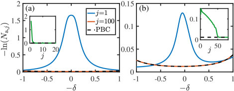
Figure 4: Indicator of amounts of local absorbed atoms, $-\ln(N_{\text{a},j})$ versus $-\delta$ on the $j$th auxiliary level when (a) $J=0$ and (b) $J=-0.05$. The insets plot $-\ln(N_{\text{a},j})$ as a function of site $j$ when $\delta=0$. The dashed black lines and other ones are calculated for a system (with the system size $N=200$) under PBCs and OBCs, respectively. Here, $J_{s}=-1$, $J_{2}=-2.5$, $g=-0.1$ and $\gamma=0.1$.

Site-resolved non-Hermitian absorption spectroscopy.—We have shown that the energy spectra in momentum space can be extracted by performing time-of-flight measurements of atoms on auxiliary levels. In this section, we will demonstrate that topological edge modes, such as zero-energy modes, in non-Hermitian systems can also be measured by probing the local occupancy $N_{\text{a},j}$ after a period of time $t$ footnote1 . We expect that the amount of absorbed atoms at boundaries exhibits a peak near $\delta=0$ for a topological system with zero-energy edge modes.

To demonstrate our method, we consider the non-Hermitian Su-Schrieffer-Heeger (SSH) model TonyLee ; Yao2018PRL1 with two sublattices $A$ and $B$ described by

$$\hat{\mathcal{H}}_{\text{s}}^{\text{NHSSH}}= \sum\nolimits_{j}[(J_{s}+g)\hat{c}_{jA}^{\dagger}\hat{c}_{jB}+(J_{s}-g)\hat{c}_{jB}^{\dagger}\hat{c}_{jA}$$

$$+J_{2}(\hat{c}_{jB}^{\dagger}\hat{c}_{j+1\,A}\!+\!\text{H.c.})-\text{i}\gamma(\hat{c}_{jA}^{\dagger}\hat{c}_{jA}\!+\!\hat{c}_{jB}^{\dagger}\hat{c}_{jB})].$$

We couple the $A$ site of each unit cell to an auxiliary level and calculate the local occupancy $N_{\text{a},j}$ in a nontrivial regime with two topological zero-energy modes localized at both edges. The site-resolved spectrum in Fig. 4 displays an absorption peak around $\delta=0$ at the left boundary, which does not exist in the bulk sites, revealing the existence of zero-energy modes. Such a feature is further illustrated by the amount of local absorbed atoms on each auxiliary level when $\delta=0$ (see the insets), showing that only the left boundary has a significant response (the right edge state can be probed if we couple $B$ sites to the auxiliary levels; see Supplemental Material S-6 B for details). We also find that by turning on $J$, the topological zero modes can be detected in a wider range near the left boundary ($j<50$) as shown in Fig. 4(b). We attribute this to the hopping between boundary sites which balances the particle distribution, while the bulk is unaffected and agrees with the results for periodic boundaries.

In summary, we have generalized the widely used radio-frequency spectroscopy to a non-Hermitian quantum system and demonstrated that it can be employed to measure both real and imaginary parts of complex energy spectra. We theoretically prove and numerically confirm that such measurement results are independent of boundary conditions even when a non-Hermitian quantum system exhibits NHSEs, thereby providing strong evidence that band structures in momentum space are experimentally measurable in a generic non-Hermitian system. In cold atom systems, we may consider either bosonic atoms, such as ⁸⁷Rb atoms, or fermionic atoms, such as ¹⁷³Yb or ⁴⁰K (see Supplemental Material S-1 C for more details). Our methods are in fact not limited to cold atom systems, but can also be used in other quantum systems, such as trapped ions WeiZhang2021PRL or solid-state spin systems Du2018Science ; Deng2021PRL ; Deng2022NC . Such a spectroscopy may also be generalized to a dissipative interacting system (see Supplemental Material S-7 for detailed discussions). Given the similarity between the radio-frequency spectroscopy and ARPES in solid-state materials, our results may also have important implications in condensed matter systems.

Note added.—Recently, we became aware of a related work where topological edge states are experimentally measured in ultracold atoms Yan2022 .

References

- (1) P. Törmä, Phys. Scr. 91, 043006 (2016).
- (2) B. Lv, T. Qian, and H. Ding, Nat. Rev. Phys. 1, 609 (2019).
- (3) C.-L. Lin, N. Kawakami, R. Arafune, E. Minamitani, and N. Takagi, J. Condens. Matter Phys. 32, 243001 (2020).
- (4) L. Pan, X. Chen, Y. Chen, and H. Zhai, Nat. Phys. 16, 767 (2020).
- (5) J. A. Sobota, Y. He, and Z.-X. Shen, Rev. Mod. Phys. 93, 025006 (2021).
- (6) C. J. Vale and M. Zwierlein, Nat. Phys. 17, 1305 (2021).
- (7) R. El-Ganainy, K. G. Makris, M. Khajavikhan, Z. H. Musslimani, S. Rotter, and D. N. Christodoulides, Nat. Phys. 14, 11 (2018).
- (8) Y. Xu, Front. Phys. 14, 43402 (2019).
- (9) D.-W. Zhang, Y.-Q. Zhu, Y. X. Zhao, H. Yan, and S.-L. Zhu, Adv. Phys. 67, 253 (2019).
- (10) Y. Ashida, Z. Gong, and M. Ueda, Adv. Phys. 69, 249 (2020).
- (11) E. J. Bergholtz, J. C. Budich, and F. K. Kunst, Rev. Mod. Phys. 93, 015005 (2021).
- (12) B. Zhen, C. W. Hsu, Y. Igarashi, L. Lu, I. Kaminer, A. Pick, S.-L. Chua, J. D. Joannopoulos, and M. Soljačić, Nature (London) 525, 354 (2015).
- (13) Y. Xu, S.-T. Wang, and L.-M. Duan, Phys. Rev. Lett. 118, 045701 (2017).
- (14) D. Leykam, K. Y. Bliokh, C. Huang, Y. D. Chong, and F. Nori, Phys. Rev. Lett. 118, 040401 (2017).
- (15) V. Kozii and L. Fu, arXiv:1708.05841 (2017).
- (16) A. A. Zyuzin and A. Y. Zyuzin, Phys. Rev. B 97, 041203(R) (2018).
- (17) H. Zhou, C. Peng, Y. Yoon, C. W. Hsu, K. A. Nelson, L. Fu, J. D. Joannopoulos, M. Soljačić, and B. Zhen, Science 359, 1009 (2018).
- (18) A. Cerjan, M. Xiao, L. Yuan, and S. Fan, Phys. Rev. B 97, 075128 (2018).
- (19) T. Yoshida, R. Peters, and N. Kawakami, Phys. Rev. B 98, 035141 (2018).
- (20) P.-L. Zhao, A.-M. Wang, and G.-Z. Liu, Phys. Rev. B 98, 085150 (2018).
- (21) J. Carlström and E. J. Bergholtz, Phys. Rev. A 98, 042114 (2018).
- (22) Z. Yang and J. Hu, Phys. Rev. B 99, 081102(R) (2019).
- (23) H.-Q. Wang, J.-W. Ruan, and H.-J. Zhang, Phys. Rev. B 99, 075130 (2019).
- (24) T. Yoshida, R. Peters, N. Kawakami, and Y. Hatsugai, Phys. Rev. B 99, 121101(R) (2019).
- (25) Ş. K. Özdemir, S. Rotter, F. Nori, and L. Yang, Nat. Mater. 18, 783 (2019).
- (26) A. Cerjan, S. Huang, M. Wang, K. P. Chen, Y. Chong, and M. C. Rechtsman, Nat. Photon. 13, 623 (2019).
- (27) K. Kawabata, T. Bessho, and M. Sato, Phys. Rev. Lett. 123, 066405 (2019).
- (28) X. Zhang, K. Ding, X. Zhou, J. Xu, and D. Jin, Phys. Rev. Lett. 123, 237202 (2019).
- (29) X.-X. Zhang and M. Franz, Phys. Rev. Lett. 124, 046401 (2020).
- (30) J. Hou, Z. Li, X.-W. Luo, Q. Gu, and C. Zhang, Phys. Rev. Lett. 124, 073603 (2020).
- (31) Z. Yang, C.-K. Chiu, C. Fang, and J. Hu, Phys. Rev. Lett. 124, 186402 (2020).
- (32) K. Wang, L. Xiao, J. C. Budich, W. Yi, and P. Xue, Phys. Rev. Lett. 127, 026404 (2021).
- (33) Y. Nagai, Y. Qi, H. Isobe, V. Kozii, and L. Fu, Phys. Rev. Lett. 125, 227204 (2020).
- (34) T. Liu, J. J. He, Z. Yang, and F. Nori, Phys. Rev. Lett. 127, 196801 (2021).
- (35) Y.-L. Tao, T. Qin, and Y. Xu, arXiv:2111.03348 (2021).
- (36) H. Wu and J.-H. An, Phys. Rev. B 105, L121113 (2022).
- (37) J. Li, A. K. Harter, J. Liu, L. de Melo, Y. N. Joglekar, and L. Luo, Nat. Commun. 10, 855 (2019).
- (38) Z. Ren, D. Liu, E. Zhao, C. He, K. K. Pak, J. Li, and G.-B. Jo, Nat. Phys. 18, 385 (2022).
- (39) S. Lapp, J. Ang’ong’a, F. A. An, and B. Gadway, New J. Phys. 21, 045006 (2019).
- (40) W. Gou, T. Chen, D. Xie, T. Xiao, T.-S. Deng, B. Gadway, W. Yi, and B. Yan, Phys. Rev. Lett. 124, 070402 (2020).
- (41) Y. Takasu, T. Yagami, Y. Ashida, R. Hamazaki, Y. Kuno, and Y. Takahashi, Prog. Theor. Exp. Phys. 2020, 12A110 (2020).
- (42) F. Ferri, R. Rosa-Medina, F. Finger, N. Dogra, M. Soriente, O. Zilberberg, T. Donner, and T. Esslinger, Phys. Rev. X 11, 041046 (2021).
- (43) R. Rosa-Medina, F. Ferri, F. Finger, N. Dogra, K. Kroeger, R. Lin, R. Chitra, T. Donner, and T. Esslinger, arXiv:2108.11888 (2021).
- (44) L. Ding, K. Shi, Q. Zhang, D. Shen, X. Zhang, and W. Zhang, Phys. Rev. Lett. 126, 083604 (2021).
- (45) S. Guo, C. Dong, F. Zhang, J. Hu, and Z. Yang, arXiv:2111.04220 (2021).
- (46) L. Zhou, H. Li, W. Yi, and X. Cui, arXiv:2111.04196 (2021).
- (47) Z.-C. Xu, Z. Zhou, E. Cheng, L.-J. Lang, and S.-L. Zhu, arXiv:2201.01216 (2022).
- (48) S. Yao and Z. Wang, Phys. Rev. Lett. 121, 086803 (2018).
- (49) T. E. Lee, Phys. Rev. Lett. 116, 133903 (2016).
- (50) Y. Xiong, J. Phys. Commun. 2, 035043 (2018).
- (51) V. M. Martinez Alvarez, J. E. Barrios Vargas, and L. E. F. Foa Torres Phys. Rev. B 97, 121401(R) (2018).
- (52) F. K. Kunst, E. Edvardsson, J. C. Budich, and E. J. Bergholtz, Phys. Rev. Lett. 121, 026808 (2018).
- (53) Q.-B. Zeng, Y.-B. Yang, and Y. Xu, Phys. Rev. B 101, 020201(R) (2020).
- (54) H. Jiang, L.-J. Lang, C. Yang, S.-L. Zhu, and S. Chen, Phys. Rev. B 100, 054301 (2019).
- (55) N. Okuma, K. Kawabata, K. Shiozaki, and M. Sato, Phys. Rev. Lett. 124, 086801 (2020).
- (56) D. S. Borgnia, A. J. Kruchkov, and R.-J. Slager, Phys. Rev. Lett. 124, 056802, (2020).
- (57) K. Zhang, Z. Yang, and C. Fang, Phys. Rev. Lett. 125, 126402 (2020).
- (58) N. Okuma and M. Sato, Phys. Rev. Lett. 126, 176601 (2021).
- (59) P. Törmä, Spectroscopies—theory, in Quantum Gas Experiments—Exploring Many-Body States, edited by P. Törmä and K. Sengstock (Imperial College Press, London, 2015).
- (60) See Supplemental Material for more details on the proof that the many-body dynamics described by the master equation is determined by the single-particle dynamics governed by the effective non-Hermitian Hamiltonian in Section S-1, the derivation of the population of the auxiliary levels based on linear response theory in Section S-2, the proof that the population is independent of boundary conditions in the thermodynamic limit in Section S-3, the influence of non-Hermitian skin effects (NHSEs) on non-Hermitian absorption spectroscopy based on the non-Hermitian Rice-Mele model in Section S-4, the analysis of the possibility of probing non-Bloch energies for systems that exhibit NHSEs and its problems in Section S-5, more results about the non-Hermitian SSH model in Section S-6, and the application of the absorption spectroscopy in interacting systems in Section S-7, which includes Refs. Prosen2008NJP ; Wang2019PRL ; Ueda2018PRX .
- (61) T. Prosen, New J. Phys. 10, 043026 (2008).
- (62) F. Song, S. Yao, and Z. Wang, Phys. Rev. Lett. 123, 170401 (2019).
- (63) Z. Gong, Y. Ashida, K. Kawabata, K. Takasan, S. Higashikawa, and M. Ueda, Phys. Rev. X 8, 031079 (2018).
- (64) T.-S. Deng, L. Pan, Y. Chen, and H. Zhai, Phys. Rev. Lett. 127, 086801 (2021).
- (65) N. Hatano and D. R. Nelson, Phys. Rev. Lett. 77, 570 (1996).
- (66) Y. Yi and Z. Yang, Phys. Rev. Lett. 125, 186802 (2020).
- (67) Y. Xu and L.-M. Duan, Phys. Rev. A 94, 053619 (2016).
- (68) Y. Xu and Y. Hu, Phys. Rev. B 99, 174309 (2019).
- (69) Y.-H. Lu, B.-Z. Wang, and X.-J. Liu, Sci. Bull. 65, 2080 (2020).
- (70) Z.-Y. Wang, X.-C. Cheng, B.-Z. Wang, J.-Y. Zhang, Y.-H. Lu, C.-R. Yi, S. Niu, Y. Deng, X.-J. Liu, S. Chen, and J.-W. Pan, Science 372, 271 (2021).
- (71) If the non-Hermitian Hamiltonian is quadratic, then we can treat each atom independently so that the local occupancy is given by Supplementary .
- (72) Y. Wu, W. Liu, J. Geng, X. Song, X. Ye, C.-K. Duan, X. Rong, and J. Du, Science 364, 878 (2018).
- (73) W. Zhang, X. Ouyang, X. Huang, X. Wang, H. Zhang, Y. Yu, X. Chang, Y. Liu, D.-L. Deng, and L.-M. Duan, Phys. Rev. Lett. 127, 090501 (2021).
- (74) Y. Yu, L.-W. Yu, W. Zhang, H. Zhang, X. Ouyang, Y. Liu, D.-L. Deng, and L.-M. Duan, arXiv:2112.13785 (2021).
- (75) Q. Liang, D. Xie, Z. Dong, H. Li, H. Li, B. Gadway, W. Yi, and B. Yan, arXiv:2201.09478 (2022).