Sticky diffusions on graphs

Abstract.

We consider diffusion processes on metric graphs with semipermeable sticky membranes in each vertex. We prove that the process is governed by a Feller semigroup and find its asymptotic behavior as diffusion’s speed increases to infinity with the same rate as permeability coefficients decreases to zero.

1. Introduction

Since around 1980 numerous papers have been published on the topic of evolution operators acting on metric graphs – see for example [6, 14], or recent survey [12] and references given there. In this context operators related to the diffusion process are one of the most extensively examined. More specifically, let $\mathcal{G}$ be a finite graph without loops, and assume that there is a Markov process on $\mathcal{G}$, which on each edge behaves like a Brownian motion with given variance. Moreover, suppose that each vertex of the graph is a semipermeable membrane with given permeability coefficients, that is for each vertex there are nonnegative numbers, describing the possibility of a particle passing through the membrane from an edge $\mathsf{e}$ to $\mathsf{f}$. In 2012, A. Bobrowski and K. Morawska [5] considered such diffusion processes on a simple graph to model synaptic depression dynamic. The results were generalized by Bobrowski in [3] to the case of arbitrary graphs. He proved that these processes are governed by strongly continuous semigroups of operators (see, for example, [7] for an introduction to the theory of semigroup of linear operators), and, moreover, that if the diffusion’s speed increases to infinity with the same rate as permeability coefficients decreases to zero (this is an example of a small parameter, or singular perturbation, problem), then there is a limit process, in the sense of Theorem 3.26 in [13], which behaves like a Markov chain on the vertices of the line graph of $\mathcal{G}$, see Figure 1.

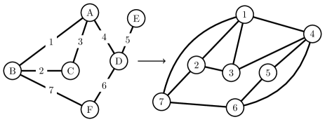
Figure 1. Diffusion on a graph $\mathcal{G}$ becomes a Markov chain on the vertices of the line graph of $\mathcal{G}$.

Because in Bobrowski’s papers the analysis takes place in the space of continuous functions on $\mathcal{G}$, the related semigroups describe dynamics of (weighted) conditional expected values of these processes. It is also worth noting that the communication between edges is based on the Fick law, or, in other words, that boundary conditions at vertices are Robin-type.

In 2014, in order to obtain the dynamics of densities of Bobrowski’s processes distributions, we considered in [9] a “dual” description of the processes with the underlying space being the $L^{1}$-type space of Lebesgue integrable functions on $\mathcal{G}$. One may wish to mimic the argument of the continuous case but this is not fully possible (the reason is that a pointwise evaluation is not a bounded functional in an $L^{1}$-type space), thus a different method is needed.

These results, in the space of continuous functions and in the $L^{1}$-type space, were improved by J. Banasiak et al. [1, 2]. Moreover, if we are interested in generation theorems only, then Banasiak’s results follow from a recent and very general scheme developed by T. Binz and K.J. Engel (in the space of continuous functions), and M. Kramar Fijavž and K.J. Engel (in the $L^{1}$-type space).

In this paper we generalize results of [3] to the case of sticky boundary conditions. We consider the process that on each edge of the underlying graph behaves as a Brownian motion, and in each vertex we put a semipermeable sticky membrane; see Example 3.59 in [13] or Appendix for detailed description of this type of boundary condition. We prove, see Theorem 2.1, that the process is governed by a Feller semigroup and, see Theorem 2.4, find its asymptotic behavior as diffusion’s speed increases to infinity with the same rate as permeability coefficients decreases to zero.

2. Sticky diffusion on a graph

Let $\mathsf{G}=(\mathsf{V},\mathsf{E})$ be a finite graph without loops, where $\mathsf{V}=\{\mathsf{v}_{1},\ldots,\mathsf{v}_{n}\}$ is the set of vertices and and $\mathsf{E}=\{\mathsf{e}_{1},\ldots,\mathsf{e}_{m}\}$ is the set of edges of $\mathsf{G}$. We arbitrarily fix an orientation of $\mathsf{G}$ and introduce the incidence matrix $\mathcal{I}=(\iota_{\mathsf{v},\mathsf{e}})_{\mathsf{v}\in\mathsf{V},\mathsf{e}\in\mathsf{E}}$ defined by

$$\iota_{\mathsf{v},\mathsf{e}}=\begin{cases}-1,&\text{$\mathsf{v}$ is the initial endpoint $\mathsf{e}_{\mathrm{init}}$ of $\mathsf{e}$},\\ +1,&\text{$\mathsf{v}$ is the terminal endpoint $\mathsf{e}_{\mathrm{term}}$ of $\mathsf{e}$},\\ 0,&\text{otherwise}.\end{cases}$$

To define a metric analogue of the discrete object $\mathsf{G}$, we assign to each edge $\mathsf{e}\in\mathsf{E}$ a closed interval, which we normalize to $[0,1]$ for simplicity. We let $\mathcal{G}$ to be the disjoint union of these intervals, that is

$$\mathcal{G}\coloneqq\bigsqcup_{\mathsf{e}\in\mathsf{E}}[0,1],$$

and denote elements of $\mathcal{G}$ by $\mathsf{e}(s)$ for all $\mathsf{e}\in\mathsf{E}$ and $s\in[0,1]$. Notice that there can be many ‘copies’ of a single vertex $\mathsf{v}\in\mathsf{V}$ in $\mathcal{G}$, and that $\mathcal{G}$ does not itself posses a graph structure – there is no information about connections between vertices. From this point of view, if we want to treat $\mathcal{G}$ as a metric graph, we need to refer to adjacency matrix $\mathcal{I}$, for example. If we endow each interval of $\mathcal{G}$ with the standard metric on $[0,1]$, then $\mathcal{G}$ becomes a disconnected compact metric space. With slight abuse of notation, we view $\mathsf{e}$ as an element of $\mathsf{E}$ as well as a connected component of $\mathcal{G}$. We parametrize each component according to the orientation of the related edge $\mathsf{e}$, and call $\mathsf{e}^{-}\coloneqq\mathsf{e}(0)$ and $\mathsf{e}^{+}\coloneqq\mathsf{e}(1)$ the left and right endpoints of (the interval related to) $\mathsf{e}$. By $C(\mathcal{G})$ we denote the space of continuous function on $\mathcal{G}$ with the standard supremum norm. This space is isometrically isomorphic to the Cartesian product $\bigtimes_{\mathsf{e}\in\mathsf{E}}C[0,1]$, where $C[0,1]$ is the space of continuous functions on $[0,1]$. Therefore, we may identify $u\in C(\mathcal{G})$ with $(u_{\mathsf{e}})_{\mathsf{e}\in\mathsf{E}}$, where $u_{\mathsf{e}}$ is a member of $C[0,1]$. Nevertheless, whenever possible, we consider $u\in C(\mathcal{G})$ as a real-valued function on a disconnected space $\mathcal{G}$, and use the edgewise identification $u=(u_{\mathsf{e}})_{\mathsf{e}\in\mathsf{E}}$ when needed. Such approach is convenient, since when we apply the positive maximum principle for Feller semigroups, we have to work in the space of real-valued continuous functions. Note also that it makes sense to speak about differentiable functions on $\mathcal{G}$, and in particular, by $C^{k}(\mathcal{G})$ we denote the space of $k$-times continuously differentiable functions on $\mathcal{G}$.

Fix $\epsilon\in(0,1]$, and for every $\mathsf{e}\in\mathsf{E}$ let $\sigma_{\mathsf{e}}$ be a positive constant. We define $\sigma\in C(\mathcal{G})$ to be the continuous function on $\mathcal{G}$, which on each edge $\mathsf{e}\in\mathsf{E}$ equals $\sigma_{\mathsf{e}}$, and consider the diffusion equation

$$\partial_{t}u(t,x)=\epsilon\sigma(x)\partial_{xx}u(t,x),\qquad t>0,\ x\in\operatorname{int}\mathcal{G},$$

where $\operatorname{int}\mathcal{G}$ is the interior of $\mathcal{G}$, which is the disjoint union of the intervals $(0,1)$, that is

$$\operatorname{int}\mathcal{G}=\bigsqcup_{\mathsf{e}\in\mathsf{E}}(0,1).$$

This means that on the edge $\mathsf{e}$ the related process behaves like a Brownian motion with variance $\epsilon\sigma_{\mathsf{e}}$.

To describe the communication between the edges, we follow [1, 2, 3, 10], and for each $\mathsf{e}\in\mathsf{E}$ we let $l_{\mathsf{e}}$ and $r_{\mathsf{e}}$ be nonnegative real numbers giving the rates at which Brownian particles pass through the membrane from the edge $\mathsf{e}$ to the edges incident in the left and right endpoints, respectively. Also, for $\mathsf{e},\mathsf{f}\in\mathsf{E}$ such that $\mathsf{e}\neq\mathsf{f}$ let $l_{\mathsf{e},\mathsf{f}}$ and $r_{\mathsf{e},\mathsf{f}}$ be nonnegative real numbers satisfying $\sum_{\mathsf{f}\neq\mathsf{e}}l_{\mathsf{e},\mathsf{f}}\leqslant l_{\mathsf{e}}$ and $\sum_{\mathsf{f}\neq\mathsf{e}}r_{\mathsf{e},\mathsf{f}}\leqslant r_{\mathsf{e}}$; the summation here is taken over all $\mathsf{f}\in\mathsf{E}$ such that $\mathsf{f}\neq\mathsf{e}$. These numbers determine the probability that after filtering through the membrane of the edge $\mathsf{e}$ a particle will enter the edge $\mathsf{f}$. More specifically, the probability that a particle after filtering through the membrane at the left endpoint $\mathsf{e}^{-}$ will enter the edge $\mathsf{f}$ equals $l_{\mathsf{e},\mathsf{f}}/l_{\mathsf{e}}$, and, by default, if $\mathsf{f}$ is not incident with the initial endpoint of $\mathsf{e}$ in $\mathsf{G}$, we put $l_{\mathsf{e},\mathsf{f}}=0$. Analogously, $r_{\mathsf{e},\mathsf{f}}/r_{\mathsf{e}}$ is the probability that after filtering through the membrane at $\mathsf{e}^{+}$ the particle will enter the edge $\mathsf{f}$, and $r_{\mathsf{e},\mathsf{f}}=0$, provided that $\mathsf{f}$ is not incident with the terminal endpoint of $\mathsf{e}$ in $\mathsf{G}$. For $\mathsf{e}\neq\mathsf{f}$ we denote by $\mathsf{f}_{\mathsf{e}}^{-}$ and $\mathsf{f}_{\mathsf{e}}^{+}$ the left and right, respectively, endpoint of $\mathsf{e}$ seen as an endpoint of $\mathsf{f}$. In other words,

$$\mathsf{f}_{\mathsf{e}}^{-}=\begin{cases}\mathsf{f}^{-},&\mathsf{f}_{\mathrm{init}}=\mathsf{e}_{\mathrm{init}},\\ \mathsf{f}^{+},&\mathsf{f}_{\mathrm{term}}=\mathsf{e}_{\mathrm{init}},\\ \text{undefined},&\text{$\mathsf{f}$ is not incident to $\mathsf{e}_{\mathrm{init}}$},\end{cases}$$

and similarly for $\mathsf{f}_{\mathsf{e}}^{+}$.

With these notations we impose for each $\mathsf{e}\in\mathsf{E}$ the following sticky transmission conditions (see Appendix for a detailed description) between the edges:

$$p_{\mathsf{e}}\partial_{xx}u(t,\mathsf{e}^{-})-p_{\mathsf{e}}^{*}\partial_{x}u(t,\mathsf{e}^{-})=\sum_{\mathsf{f}\in\mathsf{E}}\epsilon l_{\mathsf{e},\mathsf{f}}u(t,\mathsf{f}_{\mathsf{e}}^{-})-\epsilon l_{\mathsf{e}}u(t,\mathsf{e}^{-}),$$

and

$$q_{\mathsf{e}}\partial_{xx}u(t,\mathsf{e}^{+})+q_{\mathsf{e}}^{*}\partial_{x}u(t,\mathsf{e}^{+})=\sum_{\mathsf{f}\in\mathsf{E}}\epsilon r_{\mathsf{e},\mathsf{f}}u(t,\mathsf{f}_{\mathsf{e}}^{+})-\epsilon r_{\mathsf{e}}u(t,\mathsf{e}^{+}),$$

where $p_{\mathsf{e}},q_{\mathsf{e}}\in[0,1]$, $p_{\mathsf{e}}^{*}\coloneqq 1-p_{\mathsf{e}}$, $q_{\mathsf{e}}\coloneqq 1-q_{\mathsf{e}}$. By convention, if $\mathsf{f}_{\mathsf{e}}^{-}$ or $\mathsf{f}_{\mathsf{e}}^{+}$ is not defined, or, equivalently, $l_{\mathsf{e},\mathsf{f}}=0$ or $r_{\mathsf{e},\mathsf{f}}=0$, we let $l_{\mathsf{e},\mathsf{f}}u(t,\mathsf{f}_{\mathsf{e}}^{-})=0$ or $r_{\mathsf{e},\mathsf{f}}u(t,\mathsf{f}_{\mathsf{e}}^{+})=0$, respectively.

2.1. Generation theorem

We begin by considering the abstract operator related to the diffusion process. To this end, let $\epsilon\in(0,1]$, $\sigma=(\sigma_{\mathsf{e}})_{\mathsf{e}\in\mathsf{E}}$ be a positive continuous function on $\mathcal{G}$ that is constant on each edge, and $p_{\mathsf{e}},q_{\mathsf{e}}\in[0,1]$. We let $A_{\epsilon}$ to be the operator in $C(\mathcal{G})$ given by

$$A_{\epsilon}u\coloneqq\epsilon^{-1}\sigma u^{\prime\prime},\qquad u\in\operatorname{\mathcal{D}}(A_{\epsilon}).$$ (2.1)

Recall that we consider $C(\mathcal{G})$ as the space of real-valued continuous functions on the disconnected space $\mathcal{G}$, hence, $A_{\epsilon}u(x)=\epsilon^{-1}\sigma(x)u^{\prime\prime}(x)$ for all $x\in\mathcal{G}$. We define the domain of $A_{\epsilon}$ as

$$\operatorname{\mathcal{D}}(A_{\epsilon})\coloneqq\{u\in C^{2}(\mathcal{G})\colon Lu=\epsilon\Phi u\},$$ (2.2)

where $L\colon C^{2}(\mathcal{G})\to\mathbb{R}^{2\lvert\mathsf{E}\rvert}$ ($\lvert E\rvert$ is the cardinality of $E$) is given by

$$Lu\coloneqq\big{\lparen}p_{\mathsf{e}}u^{\prime\prime}(\mathsf{e}^{-})-(1-p_{\mathsf{e}})u^{\prime}(\mathsf{e}^{-}),q_{\mathsf{e}}u^{\prime\prime}(\mathsf{e}^{+})+(1-q_{\mathsf{e}})u^{\prime}(\mathsf{e}^{+})\big{\rparen}_{\mathsf{e}\in\mathsf{E}},\qquad u\in C^{2}(\mathcal{G}),$$

and $\Phi\colon C(\mathcal{G})\to\mathbb{R}^{2\lvert\mathsf{E}\rvert}$ is the bounded linear operator

$$\Phi u=(\Phi_{\mathsf{e}}^{-},\Phi_{\mathsf{e}}^{+})_{\mathsf{e}\in\mathsf{E}}\coloneqq\bigg{\lparen}\sum_{\mathsf{f}\in\mathsf{E}}l_{\mathsf{e},\mathsf{f}}u(\mathsf{f}_{\mathsf{e}}^{-})-l_{\mathsf{e}}u(\mathsf{e}^{-}),\sum_{\mathsf{f}\in\mathsf{E}}r_{\mathsf{e},\mathsf{f}}u(\mathsf{f}_{\mathsf{e}}^{+})-r_{\mathsf{e}}u(\mathsf{e}^{+})\bigg{\rparen}_{\mathsf{e}\in\mathsf{E}}$$

for all $u\in C(\mathcal{G})$. We also denote

$$\Phi_{\epsilon}\coloneqq\epsilon\Phi.$$

Theorem 2.1.

The operator $A_{\epsilon}$ given by (2.1)–(2.2) generates a Feller semigroup in $C(\mathcal{G})$. The semigroup is conservative if and only if

$$\sum_{f\in\mathsf{E}}l_{\mathsf{e},\mathsf{f}}=l_{\mathsf{e}}\qquad\text{and}\qquad\sum_{f\in\mathsf{E}}r_{\mathsf{e},\mathsf{f}}=r_{\mathsf{e}}$$ (2.3)

for all $\mathsf{e}\in\mathsf{E}$.

Before we prove Theorem 2.1 we introduce the operator $A_{0}$ as $\epsilon A_{\epsilon}$ with $\Phi=0$, that is $A_{0}u=\sigma u^{\prime\prime}$ for all $u\in\operatorname{\mathcal{D}}(A_{0})$, where

$$\operatorname{\mathcal{D}}(A_{0})\coloneqq\{u\in C^{2}(\mathcal{G})\colon Lu=0\}.$$

In other words, on each edge $\mathsf{e}$, $A_{0}$ is a (rescaled by $\sigma_{\mathsf{e}}$) copy of the generator $G_{p_{\mathsf{e}},q_{\mathsf{e}}}$ of a one-dimensional sticky diffusion on $[0,1]$ – see Appendix.

Proof.

By a well-known characterisation of Feller semigroups, see Theorem 2.2 in [8], the operator $A_{\epsilon}$ is a Feller generator if and only if it is densely defined, satisfies the positive maximum principle, and the range of $\lambda-A_{\epsilon}$ is $C(\mathcal{G})$ for some $\lambda>0$. The fact that the domain $\operatorname{\mathcal{D}}(A_{\epsilon})$ is dense in $C(\mathcal{G})$ follows by Lemma 3.6, and arguing as in [4] p. 17, it is easy to check that $A_{\epsilon}$ satisfies the positive maximum principle. Hence, we are left with proving the range condition. To this end we use Greiner’s idea of perturbing the boundary conditions, see [11, Lemma 1.4].

Let $\Lambda_{\epsilon}$ be the operator in $C(\mathcal{G})$ defined as $A_{\epsilon}$ with domain $C^{2}(\mathcal{G})$, that is $\Lambda_{\epsilon}u\coloneqq\epsilon^{-1}\sigma u^{\prime\prime}$ for all $u\in C^{2}(\mathcal{G})$, and define

$$L_{\lambda,\epsilon}\colon\mathbb{R}^{2\lvert\mathsf{E}\rvert}\to\ker(\lambda-\Lambda_{\epsilon}),\qquad L_{\lambda,\epsilon}\coloneqq(L_{|\ker(\lambda-\Lambda_{\epsilon})})^{-1}.$$

That is, $L_{\lambda,\epsilon}$ is the inverse of $L$ as restricted to $\ker(\lambda-\Lambda_{\epsilon})$. By Lemma 3.2 in Appendix such inverse exists for all $\lambda>0$ and

$$\big{\lparen}L_{\lambda,\epsilon}(a_{\mathsf{f}},b_{\mathsf{f}})_{\mathsf{f}\in\mathsf{E}}\big{\rparen}(\mathsf{e}(s))=u_{\mathsf{e}}(\mathsf{e}(s))\coloneqq c_{\mathsf{e}}\mathrm{e}^{\gamma_{\mathsf{e}}s}+d_{\mathsf{e}}\mathrm{e}^{-\gamma_{\mathsf{e}}s}$$

for all $(a_{\mathsf{f}},b_{\mathsf{f}})_{\mathsf{f}\in\mathsf{E}}\in\mathbb{R}^{2\lvert\mathsf{E}\rvert}$, $\mathsf{e}\in\mathsf{E}$, and $s\in[0,1]$, where $\gamma_{\mathsf{e}}\coloneqq\sqrt{\lambda\epsilon/\sigma_{\mathsf{e}}}$, and $c_{\mathsf{e}}$, $d_{\mathsf{e}}$ is the unique pair of real numbers satisfying (3.3) for

$$\mu\coloneqq\gamma_{\mathsf{e}},\qquad a(\mu)\coloneqq a_{\mathsf{e}}\gamma_{\mathsf{e}}^{-1},\qquad b(\mu)\coloneqq b_{\mathsf{e}}\gamma_{\mathsf{e}}^{-1}.$$

Moreover, by (3.6) there exist $\lambda_{0}>0$ and $M>0$ (that depend merely on $\epsilon$ and $\sigma$) such that

$$\lVert u_{\mathsf{e}}(\mathsf{e}(\cdot))\rVert_{C[0,1]}\leq\frac{M}{\sqrt{\lambda}}(\lvert a_{\mathsf{e}}\rvert+\lvert b_{\mathsf{e}}\rvert),\qquad\mathsf{e}\in\mathsf{E},$$

provided that $\lambda>\lambda_{0}$. This proves that $L_{\lambda,\epsilon}$ is a bounded operator $\mathbb{R}^{2\lvert\mathsf{E}\rvert}\to C(\mathcal{G})$ and its norm satisfies

$$\lVert L_{\lambda,\epsilon}\rVert\leq\frac{M^{\prime}}{\sqrt{\lambda}},\qquad\lambda>\lambda_{0}$$ (2.4)

for some $M^{\prime}>0$ depending on the norm introduced in $\mathbb{R}^{2\lvert\mathsf{E}\rvert}$. Therefore, since $\Phi_{\epsilon}$ is bounded in $C(\mathcal{G})$, there exists $\lambda_{1}>0$ such that the norm of the bounded operator $L_{\lambda,\epsilon}\Phi_{\epsilon}$ in $C(\mathcal{G})$ is less then $1$ for $\lambda>\lambda_{1}$, and consequently the operator $I_{C(\mathcal{G})}-L_{\lambda,\epsilon}\Phi_{\epsilon}$, where $I_{C(\mathcal{G})}$ is the identity operator in $C(\mathcal{G})$, is invertible.

Let $v\in C(\mathcal{G})$, and choose $\lambda>\lambda_{1}$. Set $w\coloneqq(\lambda-A_{0})^{-1}v$, which exists by Theorem 3.1, and define

$$u\coloneqq(I_{C(\mathcal{G})}-L_{\lambda,\epsilon}\Phi_{\epsilon})^{-1}w.$$

We show that $u$ belongs to $\operatorname{\mathcal{D}}(A_{\epsilon})$ and that $(\lambda-A_{\epsilon})u=v$. We have $w\in\operatorname{\mathcal{D}}(A_{0})$, and hence $u=w+L_{\lambda,\epsilon}\Phi_{\epsilon}u$ belongs to $C^{2}(\mathcal{G})$. To check that $u\in D(A_{\epsilon})$, note that

$$Lu=Lw+LL_{\lambda,\epsilon}\Phi_{\epsilon}u=0+\Phi_{\epsilon}u=\Phi_{\epsilon}u.$$

Finally,

$$A_{\epsilon}u =\Lambda_{\epsilon}w+\lambda L_{\lambda,\epsilon}\Phi_{\epsilon}u-(\lambda-\Lambda_{\epsilon})L_{\lambda,\epsilon}\Phi_{\epsilon}u$$

$$=-(\lambda-\Lambda_{\epsilon})w+\lambda w+\lambda L_{\lambda,\epsilon}\Phi_{\epsilon}u=-v+\lambda u,$$

which completes the proof of the generation part.

The semigroup generated by $A_{\epsilon}$ is conservative if and only if the function $1_{\mathcal{G}}$ that equals $1$ for every $x\in\mathcal{G}$ belongs to the domain of $A_{\epsilon}$. Since $L1_{\mathcal{G}}=0$, $1_{\mathcal{G}}\in\operatorname{\mathcal{D}}(A_{\epsilon})$ is equivalent to $\Phi 1_{\mathcal{G}}=0$, which is exactly (2.3). ∎

As a by-product of the proof we obtain the formula for the resolvent $\operatorname{\mathcal{R}}(\lambda,A_{\epsilon})$ of $A_{\epsilon}$ in terms of the resolvent $\operatorname{\mathcal{R}}(\lambda,A_{0})$ of $A_{0}$.

Corollary 2.2.

For sufficiently large $\lambda>0$ we have

$$\operatorname{\mathcal{R}}(\lambda,A_{\epsilon})u=(I_{C(\mathcal{G})}-L_{\lambda,\epsilon}\Phi_{\epsilon})^{-1}\operatorname{\mathcal{R}}(\lambda,A_{0})u,\qquad u\in C(\mathcal{G}),$$

where $L_{\lambda,\epsilon}\coloneqq(L_{|\ker(\lambda-\Lambda_{\epsilon})})^{-1}$ for

$$\Lambda_{\epsilon}u\coloneqq\epsilon^{-1}\sigma u^{\prime\prime},\qquad u\in C^{2}(\mathcal{G}).$$

2.2. Convergence

Here we examine what happens with the semigroup generated by $A_{\epsilon}$, when $\epsilon$ converges to $0^{+}$. To this end we recall (a special case of) the singular convergence theorem due to T. Kurtz (see [8, Corollary 7.7, p. 40] or [4, Theorem 42.2 and Theorem 7.1]).

Theorem 2.3.

Assume that the following conditions hold.

1. For every $\epsilon\in[0,1]$ each operator $\mathcal{A}_{\epsilon}$ is the generator of a strongly continuous semigroup in a Banach space $\mathbb{X}$, and there exists $M>0$ such that $\lVert\mathrm{e}^{t\mathcal{A}_{\epsilon}}\rVert_{\mathcal{L}(\mathbb{X})}\leq M$ for all $\epsilon\in(0,1]$ and $t\geq 0$.

2. For some (hence all) $\lambda>0$ the resolvent $R(\lambda,\epsilon\mathcal{A}_{\epsilon})$ converges strongly to the resolvent $R(\lambda,\mathcal{A}_{0})$ as $\epsilon\to 0^{+}$.

3. For every $x\in\mathbb{X}$ the limit

   $$\mathcal{P}x\coloneqq\lim_{t\to+\infty}\mathrm{e}^{t\mathcal{A}_{0}}x$$

   exists.

4. An operator $\mathcal{Q}$ generates a strongly continuous semigroup in the space

   $$\mathbb{X}_{0}\coloneqq\operatorname{range}\mathcal{P},$$

   and for some (hence all sufficiently large) $\lambda>0$ we have

   $$\lim_{\epsilon\to 0^{+}}R(\lambda,\mathcal{A}_{\epsilon})x=R(\lambda,\mathcal{Q})\mathcal{P}x,\qquad x\in\mathbb{X}.$$

Then

$$\lim_{\epsilon\to 0^{+}}\mathrm{e}^{t\mathcal{A}_{\epsilon}}x=\mathrm{e}^{t\mathcal{Q}}\mathcal{P}x$$

for all $t>0$ and $x\in\mathbb{X}$. The convergence is uniform in $t$ on compact subsets of $(0,+\infty)$, and if $x\in\mathbb{X}_{0}$, then the formula holds also for $t=0$, and the convergence is uniform in $t$ on compact subsets of $[0,+\infty)$.

We apply Kurtz’s theorem in the following setup. Let $\mathbb{X}\coloneqq C(\mathcal{G})$ and $\mathcal{A}_{\epsilon}\coloneqq A_{\epsilon}$ for every $\epsilon\in[0,1]$. Then condition (i) holds by Theorem 2.1. Moreover, by Theorem 3.1, we obtain

$$\lim_{t\to+\infty}\mathrm{e}^{tA_{0}}u=\lim_{\lambda\to 0^{+}}\lambda\operatorname{\mathcal{R}}(\lambda,A_{0})u=Pu,\qquad u\in C(\mathcal{G}),$$ (2.5)

for

$$P\coloneqq(P_{p_{\mathsf{e}},q_{\mathsf{e}}})_{\mathsf{e}\in\mathsf{E}},$$ (2.6)

establishing (iii). Therefore, we are left with choosing appropriate $\mathcal{Q}$ and proving (ii), (iv).

To this end for each $\mathsf{e}\in\mathsf{E}$ we define the operator $Q_{\mathrm{e}}\colon C(\mathcal{G})\to C[0,1]$ in the following way. If $p_{\mathsf{e}}=1$ and $q_{\mathsf{e}}=1$, then

$$Q_{\mathsf{e}}u(x)\coloneqq(1-x)\Phi_{\mathsf{e}}^{-}u+x\Phi_{\mathsf{e}}^{+}u,\qquad u\in C(\mathcal{G}),\ x\in[0,1].$$

On the other, if $p_{\mathsf{e}}\neq 1$ or $q_{\mathsf{e}}\neq 1$, then

$$Q_{\mathsf{e}}u\coloneqq\frac{1}{1-p_{\mathsf{e}}q_{\mathsf{e}}}(q_{\mathsf{e}}^{*}\Phi_{\mathsf{e}}^{-}u+p_{\mathsf{e}}^{*}\Phi_{\mathsf{e}}^{+}u),\qquad u\in C(\mathcal{G}),$$

where the right-hand side is identified with the constant function on $\mathsf{e}$. Now we define the operator $Q\colon C(\mathcal{G})\to C(\mathcal{G})$ by the formula

$$Q\coloneqq\sigma(Q_{\mathsf{e}})_{\mathsf{e}\in\mathsf{E}}=(\sigma_{\mathsf{e}}Q_{\mathsf{e}})_{\mathsf{e}\in\mathsf{E}}.$$ (2.7)

Finally, in order to characterize $\mathbb{X}_{0}=\operatorname{range}P$, note that $\operatorname{range}P_{p_{\mathsf{e}},q_{\mathsf{e}}}=\mathbb{R}$, provided that $p_{\mathsf{e}}q_{\mathsf{e}}\neq 1$, and $\operatorname{range}P_{p_{\mathsf{e}},q_{\mathsf{e}}}=\mathbb{R}^{2}$, provided that $p_{\mathsf{e}}q_{\mathsf{e}}=1$. Hence

$$\operatorname{range}P\eqqcolon C_{0}(\mathcal{G}),$$

where $C_{0}(\mathcal{G})$ is isometrically isomorphic to $\mathbb{R}^{N+N_{1}}$, $N_{1}$ being the number of $\mathsf{e}\in\mathsf{E}$ such that $p_{\mathsf{e}}=q_{\mathsf{e}}=1$. Note that the operator $Q$ is bounded on $C_{0}(\mathcal{G})$. Now we are ready to state the main result.

Theorem 2.4.

Let $A_{\epsilon}$, $\epsilon\in(0,1]$ be defined by (2.1) with domain (2.2). For operators $P$ and $Q$ given by (2.6) and (2.7), respectively, it follows that

$$\lim_{\epsilon\to 0^{+}}\mathrm{e}^{tA_{\epsilon}}u=\mathrm{e}^{tQ}Pu,\qquad t>0,\ u\in C(\mathcal{G})$$

uniformly in $t$ on compact subsets of $(0,+\infty)$. Moreover, if $u\in C_{0}(\mathcal{G})$, then the formula holds also for $t=0$, and the convergence is uniform on compact subsets of $[0,+\infty)$.

To verify conditions (ii) and (iv) and consequently prove Theorem 2.4, we need the following result.

Lemma 2.5.

For sufficiently large $\lambda>0$ and all $u\in C(\mathcal{G})$ we have

$$\lim_{\epsilon\to 0^{+}}\operatorname{\mathcal{R}}(\lambda,\epsilon A_{\epsilon})u=\operatorname{\mathcal{R}}(\lambda,A_{0})u,$$

and

$$\lim_{\epsilon\to 0^{+}}\operatorname{\mathcal{R}}(\lambda,A_{\epsilon})u=\operatorname{\mathcal{R}}(\lambda,Q)Pu.$$

Proof.

We first prove the second equality. Combining Theorem 3.1 and Corollary 2.2, we are left with investigating the (strong) limit of $L_{\lambda,\epsilon}\Phi_{\epsilon}$. Let $u=(u_{\mathsf{e}})_{\mathsf{e}\in\mathsf{E}}\in C(\mathcal{G})$. Then, calculating as in the proof of Theorem 2.1, we have

$$L_{\lambda,\epsilon}\Phi_{\epsilon}u(x)=(v_{\mathsf{e}})_{\mathsf{e}\in\mathsf{E}},$$

where

$$v_{\mathsf{e}}(x)\coloneqq c_{\mathsf{e}}\mathrm{e}^{\gamma_{\mathsf{e}}x}+d_{\mathsf{e}}\mathrm{e}^{-\gamma_{\mathsf{e}}x},\qquad x\in[0,1]$$

for $\gamma_{\mathsf{e}}\coloneqq\sqrt{\lambda\epsilon/\sigma_{\mathsf{e}}}$, and $c_{\mathsf{e}}$, $d_{\mathsf{e}}$ being the unique pair of real numbers satisfying the system of linear equations (3.3) for $z\coloneqq\gamma_{\mathsf{e}}$, and $a\coloneqq\epsilon\gamma_{\mathsf{e}}^{-1}\Phi_{\mathsf{e}}^{-}u$, $b\coloneqq\epsilon\gamma_{\mathsf{e}}^{-1}\Phi_{\mathsf{e}}^{+}u$. Now, for each $\mathsf{e}\in\mathsf{E}$ we consider two cases, depending on whether $p_{\mathsf{e}}=q_{\mathsf{e}}=1$ or not.

Case 1: Assume that $p_{\mathsf{e}}\neq 1$ or $q_{\mathsf{e}}\neq 1$. Then, solving the system explicitly using Lemma 3.2 and taking the limit as $\epsilon\to 0^{+}$, we obtain that both $c_{\mathsf{e}}$ and $d_{\mathsf{e}}$ converges to $\delta_{\mathsf{e}}/2$, where

$$\delta_{\mathsf{e}}\coloneqq\lambda^{-1}\sigma_{\mathsf{e}}\frac{q_{\mathsf{e}}^{*}\Phi_{\mathsf{e}}^{-}u+p_{\mathsf{e}}^{*}\Phi_{\mathsf{e}}^{+}u}{1-p_{\mathsf{e}}q_{\mathsf{e}}}.$$

Consequently $v_{\mathsf{e}}$ converges in $C[0,1]$ to the constant function that equals $\delta_{\mathsf{e}}$ on $[0,1]$.

Case 2: Assume that $p_{\mathsf{e}}=q_{\mathsf{e}}=1$. Then, using Lemma 3.2, we have

$$v_{\mathsf{e}}(x)=\lambda^{-1}\sigma_{\mathsf{e}}\Phi_{\mathsf{e}}^{-}u\frac{\mathrm{e}^{\gamma_{\mathsf{e}}(1-x)}-\mathrm{e}^{-\gamma_{\mathsf{e}}(1-x)}}{\mathrm{e}^{\gamma_{\mathsf{e}}}-\mathrm{e}^{-\gamma_{\mathsf{e}}}}+\lambda^{-1}\sigma_{\mathsf{e}}\Phi_{\mathsf{e}}^{+}u\frac{\mathrm{e}^{\gamma_{\mathsf{e}}x}-\mathrm{e}^{-\gamma_{\mathsf{e}}x}}{\mathrm{e}^{\gamma_{\mathsf{e}}}-\mathrm{e}^{-\gamma_{\mathsf{e}}}},\qquad x\in[0,1],$$

and taking $\epsilon\to 0^{+}$, we see that $v_{\mathsf{e}}$ converges in $C[0,1]$ to the function

$$x\mapsto(1-x)\lambda^{-1}\sigma_{\mathsf{e}}\Phi_{\mathsf{e}}^{-}u+x\lambda^{-1}\sigma_{\mathsf{e}}\Phi_{\mathsf{e}}^{+}u.$$

Combining Case 1 and Case 2 we see that $L_{\lambda,\epsilon}\Phi_{\epsilon}$ converges in $C(\mathcal{G})$ to $\lambda^{-1}Q$ as $\epsilon\to 0^{+}$. Hence (recall that the norm of $L_{\lambda,\epsilon}$ is uniformly bounded in $\epsilon$, see (2.4)), by (2.5) we obtain

$$\lim_{\epsilon\to 0^{+}}\operatorname{\mathcal{R}}(\lambda,A_{\epsilon})u =\lambda^{-1}\lim_{\epsilon\to 0^{+}}(I_{C(\mathcal{G})}-L_{\lambda,\epsilon}\Phi_{\epsilon})^{-1}Pu$$

$$=\lambda^{-1}(I_{C(\mathcal{G})}-\lambda^{-1}Q)^{-1}Pu$$

$$=(\lambda-Q)^{-1}Pu$$

for all $u\in C(\mathcal{G})$, which completes the proof of the second part of the lemma.

The first part follows similarly from the identity (obtained in the same way as Corollary 2.2)

$$\operatorname{\mathcal{R}}(\lambda,\epsilon A_{\epsilon})=\operatorname{\mathcal{R}}(1,L_{\lambda,1}\Phi_{\epsilon})\operatorname{\mathcal{R}}(\lambda,A_{0}),$$

which holds for sufficiently large $\lambda>0$. ∎

3. Appendix: One-dimensional sticky diffusion

Fix $p,q\in[0,1]$ and consider the linear operator $G_{p,q}$ in $C[0,1]$ given by

$$G_{p,q}f\coloneqq f^{\prime\prime},\qquad f\in D(G_{p,q})$$

with domain $D(G_{p,q})$ consisting of functions $f\in C^{2}[0,1]$ satisfying boundary conditions

$$pf^{\prime\prime}(0)-p^{*}f^{\prime}(0)=qf^{\prime\prime}(1)+q^{*}f^{\prime}(1)=0,$$ (3.1)

where

$$p^{*}\coloneqq 1-p,\qquad q^{*}\coloneqq 1-q.$$

We prove that $G_{p,q}$ is the generator of a Feller semigroup in $C[0,1]$. The stochastic process related to $G_{p,q}$, in the sense of Theorem 3.15 in [13], may be described as follows. Inside $(0,1)$ the process behaves like a Brownian motion with variance $1$. When a Brownian particle hits $0$, then the behaviour depends on $p$:

• If $p=0$, then the barrier at $0$ is reflecting, and the particle bounces back to $(0,1)$. The time that this particle spends at $0$ is of measure zero with respect to the Lebesgue measure, however, it has a positive measure with respect to the Lévy local time $t^{+}$, see [5, Section 4] and the references given there.

• If $p=1$, then the barrier at $0$ is absorbing, and the particle stays at $0$ forever.

• If $p\in(0,1)$, then the barrier at $0$ is sticky, and the particle stays at $0$ for some time depending on $p$. In contradistinction to the case $p=0$, the time has positive Lebesgue measure and increases with $p$, see the first displayed formula after (3.42) in [13, p. 128].

We call $p$ a stickiness coefficient at $0$. Similar description is valid for the barrier at $1$ and the stickiness coefficient $q$.

It is also possible to describe the behaviour of the process governed by $G_{p,q}$ as the time increases. To this end we introduce $P_{p,q}$ as the bounded linear operator in $C[0,1]$ defined for $p\neq 1$ and $q\neq 1$ by

$$P_{p,q}f\coloneqq\frac{pq^{*}f(0)+p^{*}qf(1)+p^{*}q^{*}\int_{0}^{1}f}{pq^{*}+p^{*}q+p^{*}q^{*}},\qquad f\in C[0,1];$$

here the right-hand side is identified with the constant function. For $p=q=1$ we additionally set

$$P_{1,1}f(x)\coloneqq(1-x)f(0)+xf(1),\qquad f\in C[0,1],\ x\in[0,1].$$

Note that for all $p,q\in[0,1]$ the operator $P_{p,q}$ is a projection, that is $P_{p,q}^{2}=P_{p,q}$.

The main result concerning one-dimensional diffusion with sticky barriers is as follows.

Theorem 3.1.

The operator $G_{p,q}$ generates a conservative, bounded analytic Feller semigroup in $C[0,1]$ of angle $\pi/2$, and

$$\lim_{t\to+\infty}\mathrm{e}^{tG_{p,q}}f=P_{p,q}f,\qquad f\in C[0,1].$$ (3.2)

Before we prove Theorem 3.1 we first state some auxiliary results. By $\mathbb{C}_{+}$ we denote the right-half of the complex plane, that is

$$\mathbb{C}_{+}\coloneqq\{\lambda\in\mathbb{C}\colon\operatorname{Re}\lambda>0\}.$$

Lemma 3.2.

For every $\mu\in\mathbb{C}_{+}$, $p,q\in[0,1]$ and functions $a,b\colon\mathbb{C}_{+}\to\mathbb{C}$, the linear system

$$\begin{bmatrix}p\mu-p^{*}&p\mu+p^{*}\\ \mathrm{e}^{\mu}\lparen q\mu+q^{*}\rparen&\mathrm{e}^{-\mu}\lparen q\mu-q^{*}\rparen.\end{bmatrix}\begin{bmatrix}c_{\mu}\\ d_{\mu}\end{bmatrix}=\begin{bmatrix}a(\mu)\\ b(\mu)\end{bmatrix}$$ (3.3)

has a unique complex solution $(c_{\mu},d_{\mu})$ given by

$$c_{\mu}=\frac{(p\mu+p^{*})b(\mu)-\mathrm{e}^{-\mu}(q\mu-q^{*})a(\mu)}{\mathrm{e}^{\mu}(p\mu+p^{*})(q\mu+q^{*})-\mathrm{e}^{-\mu}(p\mu-p^{*})(q\mu-q^{*})}$$ (3.4)

and

$$d_{\mu}=\frac{\mathrm{e}^{\mu}(q\mu+q^{*})a(\mu)-(p\mu-p^{*})b(\mu)}{\mathrm{e}^{\mu}(p\mu+p^{*})(q\mu+q^{*})-\mathrm{e}^{-\mu}(p\mu-p^{*})(q\mu-q^{*})}$$ (3.5)

Moreover,

$$c_{\mu}=O(\lvert a(\mu)\rvert\mathrm{e}^{-2\operatorname{Re}\mu}+\lvert b(\mu)\rvert\mathrm{e}^{-\operatorname{Re}\mu}),\qquad d_{\mu}=O(\lvert a(\mu)\rvert+\lvert b(\mu)\rvert\mathrm{e}^{-\operatorname{Re}\mu})$$ (3.6)

as $\operatorname{Re}\mu\to+\infty$.

Proof.

A little bit of algebra shows that the determinant $D_{\mu}$ of the system equals

$$\mathrm{e}^{-\mu}(p\mu+p^{*})(q\mu+q^{*})\big{[}H_{p}(\mu)H_{q}(\mu)-\mathrm{e}^{2\mu}\big{]},$$ (3.7)

where

$$H_{r}(z)\coloneqq\frac{rz-1+r}{rz+1-r},\qquad r\in[0,1],\ z\in\mathbb{C}_{+}.$$

We have

$$\lvert H_{r}(z)\rvert\leq 1,\qquad r\in[0,1],\ z\in\mathbb{C}_{+}.$$

Indeed, this is trivial for $r=0$, and for fixed $r\in(0,1]$ the function $H_{r}$ is (a restriction of) the Möbius transformation that maps $\mathbb{C}_{+}$ onto the open unit ball in $\mathbb{C}$. Therefore, by (3.7) it follows that

$$\lvert D_{\mu}\rvert\geq\mathrm{e}^{-\operatorname{Re}\mu}\lvert p\mu+p^{*}\rvert\lvert q\mu+q^{*}\rvert(\mathrm{e}^{2\operatorname{Re}\mu}-1)>0,$$

where in the last inequality we used the fact that $\operatorname{Re}\mu>0$. Hence the system has a unique solution, and the remaining part of the lemma follows by applying Cramer’s rule. ∎

We are ready to prove that the resolvent of $G_{p,q}$ exists. To this end, for every $\lambda\in\mathbb{C}$ we define the function $\mathrm{e}_{\lambda}$ in $C[0,1]$ by

$$\mathrm{e}_{\lambda}(x)\coloneqq\mathrm{e}^{\lambda x},\qquad x\in[0,1].$$

Moreover, for $\lambda\in\mathbb{C}\setminus\{0\}$ and $f\in C[0,1]$ we introduce $h_{\lambda}=h_{\lambda,f}\in C[0,1]$ by the formula

$$h_{\lambda}(x)\coloneqq\frac{1}{2\lambda}\int_{0}^{1}\mathrm{e}^{-\lambda\lvert x-y\rvert}f(y)\mathop{}\!\mathrm{d}y,\qquad x\in[0,1].$$

Lemma 3.3.

The resolvent set of $G_{p,q}$ contains $\mathbb{C}\setminus(-\infty,0]$ and

$$R(\lambda^{2},G_{p,q})f=c_{\lambda}\mathrm{e}_{\lambda}+d_{\lambda}\mathrm{e}_{-\lambda}+h_{\lambda},\qquad\lambda\in\mathbb{C}_{+},\ f\in C[0,1],\qquad$$ (3.8)

where $c_{\lambda}$ and $d_{\lambda}$ are given by (3.4)-(3.5) with

$$a(\lambda)\coloneqq pf(0)\lambda^{-1}-h_{\lambda}(0)(p\lambda-p^{*}),\qquad b(\lambda)\coloneqq qf(1)\lambda^{-1}-h_{\lambda}(1)(q\lambda-q^{*}).$$ (3.9)

Proof.

Since each complex number in $\mathbb{C}\setminus(-\infty,0]$ has a unique square root with positive real part, to prove that $\rho(G_{p,q})$ contains $\mathbb{C}\setminus(-\infty,0]$ it is enough to show that the resolvent $R(\lambda^{2},G_{p,q})$ exists for all $\lambda\in\mathbb{C}_{+}$. Hence, fix $\lambda\in\mathbb{C}_{+}$ and let $f\in C[0,1]$. Observe that the function $h_{\lambda}$ belongs to $C^{2}[0,1]$ and $\lambda^{2}h_{\lambda}-h_{\lambda}^{\prime\prime}=f$. Therefore, each $g\in C^{2}[0,1]$ satisfying $\lambda^{2}g-g^{\prime\prime}=f$ may be written in the form

$$g=c_{\lambda}\mathrm{e}_{\lambda}+d_{\lambda}\mathrm{e}_{-\lambda}+h_{\lambda}$$

for some $c_{\lambda},d_{\lambda}\in\mathbb{C}$. It follows that $g$ belongs to $D(G_{p,q})$, see (3.1), if and only if (3.3) holds with $a$ and $b$ as in (3.9). Consequently, Lemma 3.2 implies that $g\in D(G_{p,q})$ for the unique pair $(c_{\lambda},d_{\lambda})$ given by (3.4)-(3.5) with $a$ and $b$ as in (3.9). Moreover, there is an $M=M(\lambda)>0$ such that $\lVert g\rVert_{C[0,1]}\leq M\lVert f\rVert_{C[0,1]}$, which proves that $\lambda^{2}$ belongs to the resolvent set of $G_{p,q}$ and $R(\lambda^{2},G_{p,q})=g$. ∎

Using the explicit formula obtained in Lemma 3.3, we calculate the strong limit of the resolvent $R(\lambda,G_{p,q})$ as $\lambda$ converges to $0$.

Proposition 3.4.

We have

$$\lim_{\lambda\to 0}\lambda R(\lambda,G_{p,q})f=P_{p,q}f,\qquad f\in C[0,1],$$

in $C[0,1]$, where the limit is taken over $\lambda\in\mathbb{C}\setminus(-\infty,0]$.

Proof.

By the same reason as in the beginning of the proof of Lemma 3.3, it suffices to find the limit of $\lambda^{2}R(\lambda^{2},G_{p,q})f$ as $\lambda\to 0$ in $\mathbb{C}_{+}$. Furthermore, since $\lambda^{2}h_{\lambda}$ converges to zero as $\lambda\to 0$, by (3.8) we are left with calculating the limit of $\lambda^{2}(c_{\lambda}\mathrm{e}_{\lambda}+d_{\lambda}\mathrm{e}_{-\lambda})$.

We split the proof into two cases depending on whether both barriers are absorbing, that is $p=q=1$, or not.

Case 1: Suppose $p\neq 1$ or $q\neq 1$. We have

$$h_{\lambda}(0)=\frac{1}{2\lambda}\int_{0}^{1}(1+O(\lambda))f(x)\mathop{}\!\mathrm{d}x=\frac{1}{2\lambda}\int_{0}^{1}f+O(1),$$

and similarly

$$h_{\lambda}(1)=\frac{1}{2\lambda}\int_{0}^{1}f+O(1);$$

here, and in what follows in the proof, when we use the big-O notation we always mean “as $\lambda\to 0$ in $\mathbb{C}_{+}$.” Hence, we may rewrite $a(\lambda)$ and $b(\lambda)$ given by (3.9) in the asymptotic form

$$a(\lambda)=\frac{pf(0)}{\lambda}+\frac{p^{*}}{2\lambda}\int_{0}^{1}f+O(1),\qquad b(\lambda)=\frac{qf(1)}{\lambda}+\frac{q^{*}}{2\lambda}\int_{0}^{1}f+O(1).$$

Denoting by $D_{\lambda}$ the determinant of the coefficient matrix in (3.3), we have

$$\lambda c_{\lambda} =\frac{-\mathrm{e}^{-\lambda}pq^{*}f(0)-\mathrm{e}^{-\lambda}\frac{p^{*}q^{*}}{2}\int_{0}^{1}f-p^{*}qf(1)-\frac{p^{*}q^{*}}{2}\int_{0}^{1}f+O(\lambda)}{D_{\lambda}}$$

$$=-\frac{pq^{*}f(0)+p^{*}qf(1)+p^{*}q^{*}\int_{0}^{1}f+O(\lambda)}{D_{\lambda}}.$$

Since

$$D_{\lambda}=(\mathrm{e}^{-\lambda}-\mathrm{e}^{\lambda})p^{*}q^{*}-2\lambda pq^{*}-2\lambda p^{*}q+O(\lambda^{2})=-2\lambda(p^{*}q^{*}+pq^{*}+p^{*}q)+O(\lambda^{2}),$$

this leads to

$$\lambda c_{\lambda}=\frac{1}{2\lambda}P_{p,q}f+O(1).$$

Similarly, the same relation holds with $c_{\lambda}$ replaced by $d_{\lambda}$, and consequently we easily check that

$$\lVert\lambda^{2}(c_{\lambda}\mathrm{e}_{\lambda}+d_{\lambda}\mathrm{e}_{-\lambda})-P_{p,q}f\rVert_{C[0,1]}=O(\lambda).$$

Case 2: Suppose $p=q=1$. Then by Lemma 3.3 it follows that

$$\lambda^{2}c_{\lambda}=\frac{\mathrm{e}^{-\lambda}f(0)-f(1)-\lambda^{2}\mathrm{e}^{-\lambda}h_{\lambda}(0)+\lambda^{2}h_{\lambda}(1)}{\mathrm{e}^{-\lambda}-\mathrm{e}^{\lambda}},$$

and

$$\lambda^{2}d_{\lambda}=\frac{-\mathrm{e}^{\lambda}f(0)+f(1)+\lambda^{2}\mathrm{e}^{\lambda}h_{\lambda}(0)-\lambda^{2}h_{\lambda}(1)}{\mathrm{e}^{-\lambda}-\mathrm{e}^{\lambda}}.$$

Denoting

$$E_{\lambda}(x)\coloneqq\frac{\mathrm{e}^{-\lambda x}-\mathrm{e}^{\lambda x}}{\mathrm{e}^{-\lambda}-\mathrm{e}^{\lambda}},\qquad x\in[0,1],$$

for all $x\in[0,1]$ we have

$$\lambda^{2}[c_{\lambda}\mathrm{e}_{\lambda}(x)+d_{\lambda}\mathrm{e}_{-\lambda}(x)]=[f(0)-\lambda^{2}h_{\lambda}(0)]E_{\lambda}(1-x)+[f(1)-\lambda^{2}h_{\lambda}(1)]E_{\lambda}(x).$$

Since $\sup_{x\in[0,1]}\lvert E_{\lambda}(x)-x\rvert=O(\lambda)$, this leads to

$$\lVert\lambda^{2}(c_{\lambda}\mathrm{e}_{\lambda}(x)+d_{\lambda}\mathrm{e}_{-\lambda})-P_{1,1}f\rVert_{C[0,1]}=O(\lambda),$$

which completes the proof. ∎

Proposition 3.5.

The operator $G_{p,q}$ is sectorial with angle $\pi/2$.

Proof.

By Lemma 3.3 we are left with proving that for each $\delta\in(0,\pi/2)$ there exists $M>0$ such that

$$\lVert R(\lambda,G_{p,q})\rVert_{\mathcal{L}(C[0,1])}\leq\frac{M}{\lvert\lambda\rvert},\qquad\lambda\in\Sigma_{\pi/2+\delta}.$$ (3.10)

Since the resolvent is an analytic function on the resolvent set, see [7, Proposition IV.1.3], by Proposition 3.4 it follows that the function $\lambda\mapsto\lambda\lVert R(\lambda,G_{p,q})\rVert_{\mathcal{L}(C[0,1])}$ is bounded in every bounded subset of $\Sigma_{\pi/2+\delta}$.

We estimate the resolvent “at infinity”. Note that it suffices to prove (3.10) in the sector $\Sigma_{\pi/4+\delta/2}$ with $\lambda$ replaced by $\lambda^{2}$. Let $f\in C[0,1]$ be such that $\lVert f\rVert_{C[0,1]}\leq 1$. Lemma 3.3 implies that

$$\lVert R(\lambda^{2},G_{p,q})f\rVert_{C[0,1]}\leq\lvert c_{\lambda}\rvert\mathrm{e}^{\operatorname{Re}\lambda}+\lvert d_{\lambda}\rvert+\lVert h_{\lambda}\rVert_{C[0,1]},\qquad\lambda\in\mathbb{C}_{+}.$$ (3.11)

For every $\lambda\in\Sigma_{\pi/4+\delta/2}$ we have $\operatorname{Re}\lambda\geq\cos(\pi/4+\delta/2)\lvert\lambda\rvert$, hence

$$\lVert h_{\lambda}\rVert_{C[0,1]}\leq\frac{1}{2\lvert\lambda\rvert}\sup_{x\in[0,1]}\int_{0}^{1}\mathrm{e}^{-\operatorname{Re}\lambda\lvert x-y\rvert}\mathop{}\!\mathrm{d}y=O(\lambda^{-2})$$

uniformly in $f$; here, and in what follows in the proof, when we use the big-O notation we always mean “as $\lvert\lambda\rvert\to+\infty$ in the sector $\Sigma_{\pi/4+\delta/2}$.” This leads to

$$c_{\lambda}=\frac{O(\lambda^{-2})}{\mathrm{e}^{\lambda}+O(1)}=O(\lambda^{-2}\mathrm{e}^{-\lambda}),\qquad d_{\lambda}=\frac{O(\lambda^{-2}\mathrm{e}^{\lambda})}{\mathrm{e}^{\lambda}+O(1)}=O(\lambda^{-2})$$

uniformly in $f$. Using (3.11) we obtain $\lVert R(\lambda^{2},G_{p,q})\rVert_{\mathcal{L}(C[0,1])}=O(\lambda^{-2})$ as desired. ∎

Lemma 3.6.

Let $a_{0}$, $a_{1}$, $b_{0}$ and $b_{1}$ be real numbers. For every $\epsilon>0$ there exists a function $f\in C^{2}[0,1]$ satisfying

$$f^{\prime}(0) =a_{0}, f^{\prime\prime}(0) =b_{0},$$ (3.12)

$$f^{\prime}(1) =a_{1}, f^{\prime\prime}(1) =b_{1},$$ (3.13)

and such that

$$\lVert f\rVert_{C[0,1]}\leq\epsilon.$$

Proof.

Let $f_{\gamma}\in C[0,1]$ be given by

$$f_{\gamma}(x)\coloneqq\alpha_{0}\mathrm{e}^{-\gamma x}+\beta_{0}\mathrm{e}^{-\gamma^{2}x}+\alpha_{1}\mathrm{e}^{-\gamma(1-x)}+\beta_{1}\mathrm{e}^{-\gamma^{2}(1-x)},\qquad x\in[0,1],$$ (3.14)

where $\alpha_{0}$, $\alpha_{1}$, $\beta_{0}$ and $\beta_{1}$ are real numbers. Such $f_{\gamma}$ satisfies (3.12)–(3.13) if and only if

$$\begin{bmatrix}-\gamma&-\gamma^{2}&\gamma\mathrm{e}^{-\gamma}&\gamma^{2}\mathrm{e}^{-\gamma^{2}}\\ \gamma^{2}&\gamma^{4}&\gamma^{2}\mathrm{e}^{-\gamma}&\gamma^{4}\mathrm{e}^{-\gamma^{2}}\\ -\gamma\mathrm{e}^{-\gamma}&-\gamma^{2}\mathrm{e}^{-\gamma^{2}}&\gamma&\gamma^{2}\\ \gamma^{2}\mathrm{e}^{-\gamma}&\gamma^{4}\mathrm{e}^{-\gamma^{2}}&\gamma^{2}&\gamma^{4}\end{bmatrix}\begin{bmatrix}\alpha_{0}\\ \beta_{0}\\ \alpha_{1}\\ \beta_{1}\end{bmatrix}=\begin{bmatrix}a_{0}\\ b_{0}\\ a_{1}\\ b_{1}\end{bmatrix}.$$ (3.15)

For the determinant $D_{\gamma}$ of the coefficients matrix we have

$$D_{\gamma}=-\gamma^{10}+O(\gamma^{8})\qquad\text{as $\gamma\to+\infty$}.$$

Hence, for sufficiently large $\gamma_{0}>0$, it follows that $D_{\gamma}\neq 0$ for $\gamma>\gamma_{0}$. Consequently, for all $\gamma>\gamma_{0}$ we choose $\alpha_{0}$, $\alpha_{1}$, $\beta_{0}$ and $\beta_{1}$ in such a way that $f_{\gamma}$ given by (3.14) satisfies (3.12)–(3.13). Moreover, by (3.15) it follows that

$$\alpha_{0}=\alpha_{1}=O(\gamma^{-1}),\qquad\beta_{0}=\beta_{1}=O(\gamma^{-3})\qquad\text{as $\gamma\to+\infty$.}$$

Therefore, $\lim_{\gamma\to+\infty}\lVert f_{\gamma}\rVert_{C[0,1]}=0$, which completes the proof. ∎

Proof of Theorem 3.1.

By Lemma 3.6 it follows that the operator $G_{p,q}$ is densely defined. Hence, by Proposition 3.5, it generates an analytic semigroup $\{\mathrm{e}^{tG_{p,q}}\}_{t\geq 0}$ in $C[0,1]$. We prove that $G_{p,q}$ is a Feller generator. By a well-known characterization of Feller semigroups, see [8, Theorem 2.2, p. 165], it suffices to check that $G_{p,q}$ satisfies the positive maximum principle, that is: if $f\in D(G_{p,q})$ attains the maximum at $x\in[0,1]$, then $f(x)\geq 0$ implies $G_{p,q}f(x)\leq 0$. This is clear for $x\in(0,1)$, and if $f$ attains the nonnegative maximum at $x=0$ or $x=1$, then $f^{\prime}(0)\leq 0$ or $f^{\prime}(1)\geq 0$, respectively. Thus the claim follows, since $f$ satisfies boundary conditions (3.1). Moreover, the function $1_{[0,1]}$ belongs to the domain of $G_{p,q}$ and $G_{p,q}1_{[0,1]}=0$, hence the semigroup is conservative.

To prove (3.2) note first that the limit on the left-hand side exists, which follows by the sectoriality of the semigroup and Proposition 3.4, see [4, Corollary 32.1]. Let $f\in C[0,1]$, and write

$$f=(f-P_{p,q}f)+P_{p,q}f.$$

By Proposition 3.4 we have $\lambda R(\lambda,G_{p,q})(f-P_{p,q}f)\to P_{p,q}(f-P_{p,q}f)=0$ as $\lambda$ converges to zero in $\mathbb{C}\setminus(-\infty,0]$. However, the resolvent $R(\lambda,G_{p,q})$ is the Laplace transform of the semigroup generated by $G_{p,q}$, hence

$$\lambda R(\lambda,G_{p,q})=\int_{0}^{+\infty}\mathrm{e}^{-t}\mathrm{e}^{\frac{t}{\lambda}G_{p,q}}\mathop{}\!\mathrm{d}t,$$

which implies that $\mathrm{e}^{tG_{p,q}}(f-P_{p,q}f)\to 0$ as $t\to+\infty$. Finally, because $G_{p,q}P_{p,q}f=0$ for all $p,q\in[0,1]$, we have $R(\lambda,G_{p,q})P_{p,q}f=\lambda^{-1}P_{p,q}f$. Therefore, by the Yosida approximation it follows that $\mathrm{e}^{tG_{p,q}}P_{p,q}f=P_{p,q}f$, which completes the proof. ∎

References

[1]
J. Banasiak, A. Falkiewicz, and P. Namayanja, Asymptotic state lumping in
transport and diffusion problems on networks with applications to population
problems, Math. Models Methods Appl. Sci. 26 (2016), no. 2,
215–247.
[2]
by same author, Semigroup approach to diffusion and transport problems on
networks, Semigroup Forum 93 (2016), no. 3, 427–443.
[3]
A. Bobrowski, From diffusions on graphs to Markov chains via asymptotic
state lumping, Ann. Henri Poincaré 13 (2012), no. 6, 1501–1510.
[4]
by same author, Convergence of One-Parameter Operator Semigroups,
Cambridge University Press, Cambridge, 2016.
[5]
A. Bobrowski and K. Morawska, From a PDE model to an ODE model of
dynamics of synaptic depression, Disc. and Cont. Dyn. Systems B 17
(2012), no. 6, 2313–2327.
[6]
K.J. Engel and M. Kramar Fijavž, Waves and diffusion on metric graphs
with general vertex conditions, Evol. Equ. Control Theory 8 (2019),
no. 3, 633–661.
[7]
K.J. Engel and R. Nagel, One-Parameter Semigroups for Linear
Evolution Equations, Springer-Verlag, New York, 2000.
[8]
S.N. Ethier and T.G. Kurtz, Markov Processes. Characterization and
Convergence, Wiley, New York, 1986.
[9]
A. Gregosiewicz, Asymptotic behaviour of diffusion on graphs,
Probability in Action, vol. 1 (T. Banek and E. Kozłowski, eds.), Lublin
University of Technology Press, Lublin, 2014, pp. 83–96.
[10]
by same author, Asymptotic behaviour of fast diffusions on graphs, Semigroup
Forum 101 (2020), no. 3, 619–653.
[11]
G. Greiner, Perturbing the boundary conditions of a generator, Houston
J. Math. 13 (1987), no. 2, 213–229.
[12]
M. Kramar Fijavž and A. Puchalska, Semigroups for dynamical processes
on metric graphs, Philos. Trans. Roy. Soc. A 378 (2020), no. 2185,
619–635.
[13]
T. Liggett, Continuous Time Markov Processes, American
Mathematical Society, Providence, RI, 2010.
[14]
D. Mugnolo, Semigroup Methods for Evolution Equations on
Networks, Springer, Cham, 2014.