2022
These authors contributed equally to this work.
These authors contributed equally to this work.
[1,2,3]\fnmSimon G. J. \surMochrie
[1]\orgdivIntegrated Graduate Program in Physical and Engineering Biology, \orgnameYale University, \orgaddress\streetStreet, \cityNew Haven, \postcode06511, \stateConnecticut, \countryUSA
2]\orgdivDepartment of Applied Physics, \orgnameYale University, \orgaddress\streetStreet, \cityNew Haven, \postcode06511, \stateConnecticut, \countryUSA
3]\orgdivDepartment of Physics, \orgnameYale University, \orgaddress\streetStreet, \cityNew Haven, \postcode06511, \stateConnecticut, \countryUSA
4]\orgdivDepartment of Cell Biology, \orgnameYale University, \orgaddress\streetStreet, \cityNew Haven, \postcode06511, \stateConnecticut, \countryUSA
5]\orgdivDepartment of Biomedical Engineering, \orgnameYale University, \orgaddress\streetStreet, \cityNew Haven, \postcode06511, \stateConnecticut, \countryUSA
6]\orgdivInstitute of Quantitative Biology, Biochemistry and Biotechnology, Center for Synthetic and Systems Biology, School of Biological Sciences, \orgnameUniversity of Edinburgh, \orgaddress\streetStreet, \cityEdinburgh, \postcode06511, \countryUK
Uncovering diffusive states of the yeast membrane protein, Pma1, and how labeling method can change diffusive behavior
Abstract
We present and analyze video-microscopy-based single-particle-tracking measurements of the budding yeast (Saccharomyces cerevisiae) membrane protein, Pma1, fluorescently-labeled either by direct fusion to the switchable fluorescent protein, mEos3.2, or by a novel, light-touch, labeling scheme, in which a 5 amino acid tag is directly fused to the C-terminus of Pma1, which then binds mEos3.2. The diffusivity distributions of these two populations of single particle tracks differ significantly, demonstrating that labeling method can be an important determinant of diffusive behavior. We also applied perturbation expectation maximization (pEMv2) [Physical Review E 94, 052412 (2016)], which sorts trajectories into the statistically-optimum number of diffusive states. For both TRAP-labeled Pma1 and Pma1-mEos3.2, pEMv2 sorts the tracks into two diffusive states: an essentially immobile state and a more mobile state. However, the mobile fraction of Pma1-mEos3.2 tracks is much smaller () than the mobile fraction of TRAP-labeled Pma1 tracks (). In addition, the diffusivity of Pma1-mEos3.2’s mobile state is several times smaller than the diffusivity of TRAP-labeled Pma1’s mobile state. To critically assess pEMv2’s performance, we compare the diffusivity and covariance distributions of the experimental pEMv2-sorted populations to corresponding theoretical distributions, assuming that Pma1 displacements realize a Gaussian random process. The experiment-theory comparisons for both the TRAP-labeled Pma1 and Pma1-mEos3.2 reveal good agreement, bolstering the pEMv2 approach.
keywords:
keyword1, Keyword2, Keyword3, Keyword41 Introduction
The overarching goal of this work is to carefully examine the extent to which the measured diffusive behavior of a protein of interest (POI) in a heterogeneous, biological environment can be convincingly described in terms of a limited number of discrete diffusive states, each with its own diffusive properties. Such diffusive states might correspond to the POI being bound to different binding partners or being located in different local environments. To determine the number of diffusive states, we employ the perturbation expectation maximization (pEMv2) software, an unsupervised, systems-level, machine-learning-based data analysis and classification method that sorts a heterogeneous population of single particle tracks. We then developed a method to validate the number of states found by pEMv2, based on the theoretical displacement covariance distributions. In this paper, we studied the budding yeast (Saccharomyces cerevisiae) membrane protein, Pma1 Albers1967 ; Post1972 ; Goormaghtigh1986 ; Morsomme2000 ; Malinska2003 ; Kuehlbrandt2004 ; Spira2012 ; Mason2013 ; Henderson2014 ; Athanasopoulos2019 ; Heit2021 ; Zhao2021 —in the cell membrane. For Pma1, we find that the observed population of single-molecule trajectories can be well-described in terms of just two diffusive states. One of these states corresponds to simple diffusion. The other is essentially immobile.
Spurred by the resulting two diffusive states we find, our second goal is to quantify the differences between the diffusivities and displacement covariances exhibited by Pma1, labeled in two different ways. The first labeling method —which we refer to as “TRAP labeling” —is a light-touch method in which wild-type Pma1 is replaced with a version of Pma1, in which a 5 amino acid tag is directly fused to the C-terminus of Pma1 Pratt2016 ; Oi2020 ; Hinrichsen2017 ; Oi2020Trap-Peptide ; OiProteinScience2020 . This is done in cells expressing a version of a fluorescent protein engineered to bind the tag, thus labeling Pma1. Second is the commonly used direct-labeling method, which replaces wild-type Pma1 with a Pma1-fluorescent protein (FP) direct-fusion. In many cases, the assumption that the POI’s intrinsic biological function will be unaffected by the direct addition of the FP is surely correct. However, in some cases, adding an FP to a POI can cause the modified protein to mislocalize Huh2003 or misfunction Coutu2013 ; Li2017 ; Toseland2013 ; Jensen2012 . For example, it was recently found that tagging dynamin-related protein 1 with GFP alters oligomerization dynamics, causing impaired oligomerization compared to native protein MontecinosFranjola2020 . In another study, overexpressed, membrane-targeted GFP fusion proteins were found to form organelle aggregates, therefore changing the motion of the protein being studied Lisenbee2003 . Similarly, Pma1 provides an example of a protein that is sensitive to labeling method: Yeast strains expressing direct fusions of Pma1 and the FPs, mCherry or EGFP, both exhibit compromised growth and mislocalization of Pma1-mCherry or Pma1-EGFP, respectively, to the vacuole Hinrichsen2017 . The possibility of mislocalization or misfunction of direct fusion proteins has motivated efforts to develop and deploy alternative in vivo labeling methods that are less disruptive of the protein’s localization or function Pratt2016 ; Oi2020 ; Hinrichsen2017 ; Oi2020Trap-Peptide ; OiProteinScience2020 . The different diffusive behavior of these two differently labeled proteins, (between TRAP-labeled and direct fusion proteins) that we observe, demonstrates that it may be necessary to broadly employ minimally-perturbing labeling schemes in order to fully realize and study intrinsic biological behavior in live cells.
This paper is organized as follows. In Sec. 2, we present necessary background material. Sec. 2.1 briefly summarizes what is known about Pma1. In Sec. 2.2, we review the perturbation Expectation Maximization (pEMv2) algorithm, which determines the number of unique diffusive states within a population of single particle tracks and sorts individual tracks into those states. In Sec. 2.3, we review theoretical results for probability distributions of two-dimensional displacement covariance matrix elements Bailey2021 , which can be compared to the corresponding experimental distributions.
In Sec. 3.1, we describe the yeast strains employed in this study and how samples were prepared. We describe the microscopy setup used to collect the data in Sec. 3.2, and the methods we used for single particle tracking in Sec. 3.3.
Sec. 4 presents and discusses our results. In Sec. 4.1, we present microscopy images of the strains studied. In contrast to cells where Pma1 is expressed as a fusion protein with the fluorescent proteins, mCherry and EGFP, which show defective growth and behavior, we find that cells expressing Pma1-mEos3.2 do not show a growth defect, nor does Pma1-mEos3.2 mislocalize to the vacuole. However, these gross observations do not rule out more subtle differences in behavior between Pma1-mEos3.2 and TRAP-labeled Pma1.
In Sec. 4.2, we present the experimental track length distributions of TRAP-labeled Pma1 and Pma1-mEos3.2. In both cases, we find that the track lifetime distribution decreases approximately single-exponentially in time, indicating that Pma1 is a monomer in the cell membrane, and show that the lifetime of TRAP-labeled Pma1 tracks is shorter than that of Pma1-mEos3.2. We interpret this difference in lifetime in terms of a non-zero TRAP-peptide unbinding rate, which allows us to estimate this rate to be about s-1.
To examine the differences between the diffusive behavior of TRAP-labeled Pma1 and Pma1-mEos3.2, we subjected both of these populations of trajectories to pEMv2 analysis Koo2015 ; Koo2016 ; Rey-Suarez2020 . In Sec. 4.4, we describe the application of pEMv2 to the population of TRAP-labeled Pma1 single particle trajectories. pEMv2 sorts TRAP-labeled Pma1 trajectories into two states. After analyzing the mean squared displacements of the sorted tracks in Sec. 4.5, we test the sorted populations by comparing their covariance and diffusivity distributions to the corresponding theoretical distributions. We find good agreement between pEMv2-sorted covariance distributions and theory (Sec. 4.6), bolstering the pEMv2-based approach. Next, in Sec. 4.7, we analyze the population of Pma1-mEos3.2 direct fusion tracks with pEMv2, and find that it also shows two states. However, in contrast to TRAP-labeled Pma1, where the mobile fraction is about 0.5, the fraction of Pma1-mEos3.2 direct-fusion tracks in the mobile state that is 0.1. In addition to the much reduced mobile fraction in Pma1-mEos3.2 compared to TRAP-labeled Pma1, the diffusivities of the mobile sub-populations alone appear to be different for the two labeling strategies with the mean diffusivity of the mobile sub-population of TRAP-labeled Pma1(m2s-1) being several-fold larger than the mean diffusivity of the mobile state (state 2) of Pma1-mEos3.2 (m2s-1). Direct comparison between the sorted experimental diffusivity and covariance distributions with the theoretical diffusivity and covariance distributions from Refs. Vestergaard2014 ; Bailey2021 reveals good agreement between experiment and theory in this case too. Finally, in Sec. 5, we summarize and conclude.
2 Background
2.1 Pma1
Pma1 is the most abundant protein in the plasma membrane of budding yeast (Saccharomyces cerevisiae). It is a transmembrane protein which pumps protons out of the cell and thus plays a role in regulating the pH of the cytoplasm. Pma1 is also a marker of cell aging because, interestingly, there is less Pma1 in the plasma membranes of newly-budded daughter cells, than in the membranes of their mother cell Henderson2014 . The yeast plasma membrane is laterally organized into several different membrane “compartments” or domains. As the name implies, Pma1 is the majority protein component of the membrane compartment of Pma1 (MCP). Membrane compartments, including MCP, show characteristic linear dimensions of about 0.1 m Malinska2003 ; Spira2012 , and differ from each other in their composition, size, shape, etc. Athanasopoulos2019 – MCPs are enriched in sphingolipids, as well as Pma1, and show non-compact, “network-like” shapes Spira2012 . Pma1 contains 918 amino acids, comprising four domains: a membrane domain which includes ten transmembrane -helices, a phosphorylation domain, a nucleotide-binding domain, and an actuator-domain, which experiences significant rearrangements when Pma1 cycles between the two allosteric states, activated and inhibited, involved in its enzymatic cycle. The change from Pma1’s inhibited to activated state has been proposed to be a consequence of phosphorylation of a specific Ser residue (Ser 899) and the tandem phosphorylation of a Ser/Thr pair (Ser911 and Thr912) Albers1967 ; Post1972 . Recently, two cryoelectron microscopy studies of detergent-extracted, lipid-reconstituted, hexamerically-associated Pma1 (from S. cerevisiae and Neurospora crassa) provided microscopic details of the inhibited and activated molecular structures Zhao2021 ; Heit2021 . Other studies involving in vitro reconstitution into liposomes Goormaghtigh1986 or nanodiscs Justesen2013 report that Pma1 monomers are active in proton pumping. As far as we are aware, no study has yet definitively identified the in vivo association state of Pma1.
2.2 Perturbation expectation maximization
A number of methods have been introduced for addressing particle tracks exhibiting biological heterogeneity Koo2015 ; Koo2016 ; Saxton1997 ; Savin2007 ; Monnier2015 ; Das2009 ; Slator2015 ; Zhao2019 ; Pinholt2021 . In particular, Refs. Koo2015 ; Koo2016 describe perturbation expectation maximization, pEMv2, which simultaneously analyzes a population of particle trajectories and sorts the trajectories into distinct diffusive states, each with its own diffusion properties. pEMv2 is a machine-learning approach that makes no a priori assumptions concerning the character of a diffusive state—e.g. whether it corresponds to simple diffusion or not—but rather determines each state’s diffusive properties directly from the sorted tracks.
Although pEMv2 performs well on simulations, to date it has been applied to relatively few experimental data sets Koo2016 ; Rey-Suarez2020 . To further explore pEMv2’s performance, we apply it to our experimental dataset of Pma1 single particle tracks. In particular, we compare the statistical properties of pEMv2-sorted populations, which pEMv2 asserts are homogeneous, to theoretical expectations for a population of tracks with a single set of diffusion parameters Vestergaard2014 ; Bailey2021 .
pEMv2 is described in detail in Refs. Koo2015 ; Koo2016 . In brief, it is an unsupervised, systems-level, machine-learning-based data analysis and classification method, that takes as input a heterogeneous population of single particle trajectories. It hypothesizes the existence of several different diffusive states within the population; it then determines the most likely diffusive properties of each diffusive state, while sorting each trajectory into the most likely of these diffusive states; it follows this procedure for different numbers of diffusive states, and finally picks the optimum number of diffusive states.
Specifically, for diffusive states and tracks, pEMv2 maximizes the log-likelihood of obtaining the measured tracks:
| (1) |
where is the vector of displacements along for track , is the vector of displacements along for track , is the fraction of tracks in diffusive state , is the displacement covariance matrix of diffusive state (assumed the same for and ), and
| (2) |
is the probability of realizing trajectory , given that trajectory corresponds to diffusive state , with and the determinant and inverse of , respectively, For trajectories comprising displacements in and , each of and is an -component vector and is an symmetric Toeplitz matrix. That is, pEMv2 assumes that particle displacements are multivariate Gaussian random variables. To apply pEMv2 to experimental tracks, we subdivide longer tracks into step tracks. pEMv2 maximizes iteratively by appropriately picking and the matrix elements of for each diffusive state , and by assigning each track to the most likely diffusive state.
Model selection in pEMv2—that is, picking the appropriate value of —is implemented by picking the state with the largest Bayesian Information Criterion (BIC), defined here as
| (3) |
where is the number of data points, and is the number of model parameters, equal to the sum of the number of independent covariance matrix elements, , plus the number of independent population fractions, . The log-likelihood always increases as the number of parameters, and therefore the number of states, increases. Counteracting this behavior, the second term on the right hand side of Eq. 3 penalizes a larger number of parameters, and therefore a larger number of states. Together these two contributions lead to an optimum value of .
2.3 Covariance and diffusivity distributions
According to pEMv2, its sorted populations each correspond to a single diffusive state with well-defined diffusive properties and parameters. Assuming that a given diffusive state’s displacements are a zero-mean Gaussian random variable (Eq. 2), all statistical properties of the displacements are determined solely by the mean covariance matrix. Therefore, to test pEMv2’s performance, we sought to compare the pEMv2-sorted covariance- and diffusivity-distributions to the corresponding theoretical expectations, given the experimental mean covariances.
The development of theoretical predictions for covariance- and diffusivity-distributions is described in detail in Refs. Vestergaard2014 ; Bailey2021 . In brief, for a population of two-dimensional, single-particle trajectories, each of length , and each corresponding to the same diffusive state, the probability density for a track to yield an estimate of the covariance matrix element, steps away from the diagonal, equal to , is:
| (4) |
where and for , where through .
Many experimental systems, including TRAP-labeled Pma1 and Pma1-mEos3.2, show diffusive behavior consistent with simple diffusion with experimental errors, corresponding to a symmetric, tridiagonal covariance matrix, where the only non-zero mean covariance matrix elements are on the diagonal, namely , and one away from the diagonal, namely . Each individual track yields a measurement of and , which are related to a measurement of the diffusivity, , and the static localization noise, , for that track via Vestergaard2014
| (5) |
and
| (6) |
where is the time between camera exposures and is the exposure time. The terms involving the exposure time, , correspond to motion blur, because measurement of the particle position is integrated while the shutter is open. To be clear, , , , and are random variables. Their respective means are , , , and .
Solving Eqs. 5 and 6 for and rewriting in terms of , , and , Vestergaard2014 ; Bailey2021 , we find
| (7) |
Similarly,
| (8) |
It follows that the the probability densities of the diffusivity and the static localization noise can be expressed as
| (9) |
and
| (10) |
respectively. For each of Eq. 4, Eq. 9, and Eq. 10, to provide explicit results, we calculate the determinant in the integrand as a function of and then carry out each integral over numerically.
3 Materials and Methods
3.1 Sample preparation
All measurements described in this paper employed strains of the budding yeast, Saccharomyces cerevisiae. The construction of these strains is described in detail in Hinrichsen2017 ; Hinrichsen2018 . For strains expressing a modified version of Pma1, we replaced the native chromosomal PMA1 gene with a gene encoding modified Pma1. Modified Pma1 was expressed from the endogenous PMA1 promoter, allowing us to study behavior at endogenous expression levels.
For our microscopy experiments, overnight cultures were grown in synthetic defined (SD) media, with sucrose and raffinose. These starter cultures were diluted into fresh media, containing galactose, to obtain a final OD. Growth was then continued at C for a further 8 hrs. Cells from these cultures were then imaged as follows: 1 mg/mL of concanavalin A (conA) was applied to a clean cover slip, and incubated at room temperature for 10 minutes. Then, 0.5-1.0 mL of fresh milli-Q water was used to rinse off the excess conA. Next, the yeast culture, previously vortexed for approximately s to separate any cell clusters, was added to the conA-coated cover slip and incubated at room temperature for an additional 10 minutes. Excess, unbound cells were rinsed from the cover slip, which was then sealed to a microscope slide using a 1:1:1 ratio mixture of Vaseline, lanolin and paraffin wax (VALAP).
3.2 Microscopy
Microscopy measurements to track the motions of individual molecules of TRAP-labeled Pma1 and Pma1-mEos3.2 were carried out using the custom-built microscope, described in Ref. Zhang2017 , which has both total-internal reflection fluorescence (TIRF) and photo-activation localization microscopy (PALM) capabilities. We employed a nm-wavelength laser to switch mEos3.2 into its red state and a nm-wavelength laser for imaging of switched mEos3.2. As noted previously, Pma1 is the most abundant yeast membrane protein. Therefore, switching a subset of the population into mEos3.2’s red fluorescent state ensures sufficiently isolated, and therefore resolvable, individual trajectories for Pma1-mEos3.2, that are suitable for unambiguous single particle tracking. The trajectories reported and analyzed in this paper were collected under conditions of TIRF illumination, which restricted switching and fluorescence excitation to the portion of a cell’s membrane in close proximity to the coverslip. In addition, however, a limited quantity of wide-field PALM data were collected to visually assess the extent to which PALM signal is associated with the cell membrane. The intensity of the nm-wavelength laser was manually adjusted during the experiments to ensure a sufficient signal rate throughout the duration of data acquisition. The fields-of-view imaged were pixels, with square pixels, each spanning nm on a side. Images were collected at a rate of frames per second (fps), corresponding to s. The exposure time was also s. A custom, reflection-based autofocusing system was deployed during data acquisition to maintain the microscope focus.
| TRAP-peptide- | Pma1- | |
| labeled Pma1 | mEos3.2 | |
| Number of | 14 | 20 |
| cells studied | ||
| Number | 59226 | 20253 |
| of tracks | ||
| Number of | 60000 | 60000 |
| movie frames |
3.3 Single particle tracking
Single particle tracking was accomplished using a locally-customized Matlab version (The MathWorks, Inc.) of the software, described in Ref. Crocker1996 , initially resulting in a number of candidate localizations in each movie frame. To achieve our final set of localizations, we manually segmented brightfield images to find cells and excluded any (apparent) localizations outside cells. We also excluded localizations with standard deviations less than 0.5 pixels or more than 3.5 times the mean standard deviation of the population of localizations. Finally, to construct single-particle trajectories, spanning multiple movie frames—i.e. spanning time—we insisted that the maximum number of pixels that a particle can move between successive frames is 2 pixels, and that the maximum number of frames for which a particle can transiently disappear and still be considered part of a specific trajectory is 1 frame.
4 Results and Discussion
4.1 Microscopy
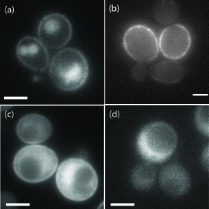
Fig. 1(a) shows wide-field fluorescence microscopy images of cells expressing a Pma1-mCherry direct fusion. Apparent in this image is a bright halo of fluorescence intensity at the cell periphery, corresponding to the localization of Pma1-mCherry to the cell membrane. Also apparent in this image is fluorescence intensity originating from regions inside the cell, corresponding to mislocalization of Pma1-mCherry to vacuoles. Evidently, the fusion of mCherry to Pma1 causes Pma1’s behavior to diverge significantly from it intrinsic behavior, which does not involve localization to vacuoles. Fig. 1(b) shows cells expressing a Pma1-mEos3.2 direct fusion. In this case also, there is a halo of fluorescence intensity at the cells’ periphery, corresponding to the localization of Pma1-mEos3.2 to the cell membrane. However, in this case, there is no mislocalization to vacuoles. Fig. 1(c) shows cells with TRAP-labeled Pma1, i.e. cells expressing both Pma1-MEEVF and TRAP-mEos3.2. In this case too, there is a halo at the cell membrane, indicating the presence of the Pma1-MEEVF-TRAP-mEos3.2 complex localized to the membrane, consistent with strong MEEVF-TRAP binding, for which Ref. Pratt2016 estimated the dissociation constant to be nM. In Fig. 1(c), fluorescence intensity also originates within the cell, corresponding to free TRAP-mEos3.2 in solution. Finally, Fig. 1(d) shows cells expressing TRAP-mEos3.2 but with unmodified Pma1. As expected, there is no longer an intensity halo at the cells’ periphery, because the TRAP-mEos3.2’s MEEVF binding partner is absent from Pma1 or anywhere else.
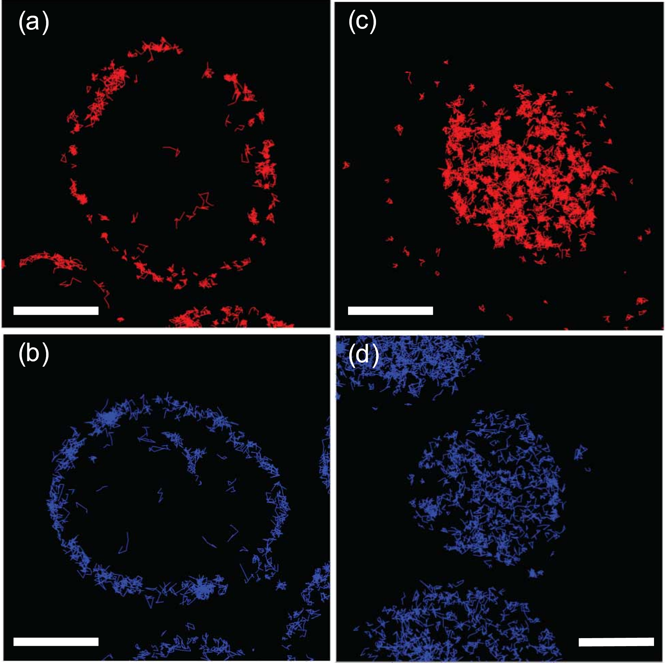
For the images in Fig. 1(b-d), mEos3.2 was visualized through its unswitched green fluorescence. However, mEos3.2 can be switched by exposure to 405 nm wavelength light into a red fluorescent state. Fig. 2(a-b) depicts trajectories of switched, red-emitting proteins containing four or more steps obtained from movies collected under 565-nm-illumination from cells with (a) Pma1-mEos3.2 and (b) TRAP-labeled Pma1. In both cases, the spatial distribution of trajectories clearly outlines the periphery of the cell that intersects the focal plane. There is no obvious difference in the spatial distribution of the tracks obtained for Pma1-mEos3.2, which we expect to be strictly confined to the cell membrane, and tracks obtained for TRAP-labeled Pma1. Initially, it may seem surprising that there are no trajectories corresponding to the cytocellular fluorescence apparent in Fig. 1(c), which depicts the same yeast strain as Fig. 2(b). However, we expect that an unbound TRAP-mEos3.2, freely and rapidly diffusing in the cytosol, would yield either a localization in just a single movie frame or a very short track at most. We infer, therefore, that trajectories with four or more steps in cells with TRAP-peptide labeling overwhelmingly must correspond to labeled Pma1 in the cell membrane, and not to unbound MEEVF-mEos3.2 in the cytosol.
More generally, the observation that unbound TRAP-mEos3.2 may be eliminated from consideration by insisting on sufficiently long tracks suggests a possible general strategy for imaging TRAP-labeled POIs Oi2020 ; Oi2021 , namely to insist that tracks endure for some minimum number of time steps. In this case, the fluorescence from unbound TRAP-FPs may be less of a problem for imaging than it might originally have seemed.
Fig. 2(c-d) shows trajectories also containing four or more steps, obtained from PALM movies collected with TIRF illumination, from cells with (c) Pma1-mEos3.2 and (d) TRAP-labeled Pma1. For both labeling methods, tracks appear largely confined to roughly circular regions. Because the tracks are derived from TIRF data, so that we expect to visualize only tracks close to the cover slide, we identify each roughly-circular region as the area of the cell in contact with the cover slide. Apparent tracks outside these regions were eliminated from further consideration. Because all of these trajectories involve four or more steps and because they were acquired through TIRF, we are confident that overwhelmingly they correspond to TRAP-labeled Pma1 and not freely-diffusing TRAP-mEos3.2. Although wide-field PALM measurements were important for establishing the conditions necessary to examine TRAP-labeled Pma1, in the remainder of the paper, we focus solely on the two-dimensional trajectories collected with TIRF illumination, in order to avoid any ambiguities associated with the sideways view of membrane-based trajectories acquired in wide-field.
4.2 Distribution of track lengths
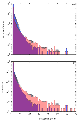
Fig. 3 displays the number of tracks versus track length on linear-logarithmic axes for both TRAP-labeled Pma1 (blue) and Pma1-mEos3.2 (pink). Evidently, for both labeling methods, the number of tracks is a monotonically decreasing function of the number of steps in the track. The track length distribution is equivalent to the distribution of fluorescent state lifetimes, because the product of the number of steps in a track and duration of a step corresponds to the lifetime of the corresponding FP(s). The behavior of the lifetime distribution clearly indicates that each of the observed tracks corresponds to a single FP, i.e., these are monomer tracks. In contrast to the observations, the lifetime distribution for a protein complex, which includes several FPs moving together, is expected to start at zero, then increase to a peak at non-zero time, before decreasing to zero again at large times. This prediction is readily understood in the case of a monomer lifetime distribution given by – a simple exponential with a characteristic rate, . Then, for an -mer comprising independent monomers, the lifetime distribution is readily shown to be . With increasing , this -mer lifetime distribution indeed starts at zero at , then increases to a peak at , before decreasing to zero again at large times, as advertized.
Although the tracks of both TRAP-labeled Pma1 and Pma1-mEos3.2 correspond to monomers, there is nevertheless a clear difference in the track length distribution between the two methods with the direct fusion showing more long tracks than TRAP-labeled Pma1. This observation is consistent with the interpretation that when Pma1 is directly bound to the FP, the lifetime of the signal is limited by photobleaching, whereas when Pma1 is labeled by the TRAP-peptide pair, the lifetime is determined by a combination of photobleaching and the lifetime of TRAP-MEEVF binding. Thus, we expect shorter lifetimes for TRAP-labeled Pma1 than for Pma1-mEos3.2. In fact, the normalized distribution of TRAP-labeled Pma1 track lengths (Fig. 3(b)) falls a factor of below that of Pma1-mEos3.2 for a track length of about 15, suggesting that the mean lifetime of the MEEVF-TRAP bond is about 0.15 s. Equivalently, the MEEVF-TRAP unbinding rate is about 6 s-1.
4.3 Population-averaged diffusivity distributions
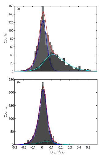
Fig. 4 compares population-averaged, diffusivity distributions, calculated on the basis of Eq. 7, for (a) the population of TRAP-labeled Pma1 tracks and (b) the population of Pma1-mEos3.2 tracks. In the figure, the overall diffusivity distributions of these populations are shown as the light-grey histograms. Although both protein variants’ overall diffusivity distributions are peaked near zero, the Pma1-mEos3.2’s diffusivity distribution is largely confined within m2/s. By contrast, TRAP-labeled Pma1’s diffusivity distribution shows a large diffusivity tail, extending beyond m2/s. Evidently, there is a substantial, qualitative difference between the overall diffusivity distribution of Pma1-mEos3.2 and the diffusivity distribution of TRAP-labeled Pma1. This result shows directly, without any further detailed analysis, that labeling strategy significantly affects the dynamics of membrane-bound Pma1, with unknown consequences to Pma1’s biological roles. Because TRAP-labeling minimally modifies the protein of interest, and direct fusions with other fluorescent proteins causes growth defects and Pma1 mislocalization, our assumption is that TRAP-labeled Pma1 more closely represents the intrinsic biological behavior of wild-type Pma1, than does Pma1-mEos3.2.
4.4 pEMv2 sorts TRAP-labeled Pma1 trajectories into two diffusive states
pEMv2 is most reliable for a large number of long trajectories Koo2016 . By contrast, experimentally, as illustrated in Fig. 3, the number of available tracks decreases rapidly with increasing track length. Therefore, to explore pEMv2’s performance and consistency over the range of available track lengths and numbers of tracks, we chose to partition each dataset into populations of trajectories with track lengths of 5, 6, 7, 8, 9, 10, 11, 12, and 15 steps. For the entire population of tracks, we find that the mean covariances, , are very close to zero for all for all track lengths. Therefore, for simplicity we chose to set these covariances identically equal to zero when running pEMv2. The statement that for is equivalent to the statement that labeled Pma1 undergoes simple diffusion in the presence of experimental errors.
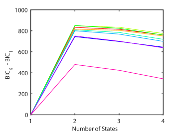
We carried out a pEMv2-analysis for each population of different-length trajectories. Fig. 5 plots the values of BICBIC1 returned by pEMv2 versus the number of diffusive states, , for track lengths of 5, 6, 7, 8, 9, 10, 11, 12 and 15 steps. For each track length, the BIC achieves a maximum for , irrespective of track length, indicating that pEMv2 robustly supports two subpopulations, namely state 1 and state 2 – with distinct diffusive properties.
| Track Length | ||||||||||||||||||
|---|---|---|---|---|---|---|---|---|---|---|---|---|---|---|---|---|---|---|
| 5 | 0.0065 | 5.79 | -0.0032 | 5.10 | 0.0013 | 0.0015 | 0.0032 | 4.27 | 0.0124 | 8.72 | -0.0013 | 8.58 | 0.2462 | 0.0041 | 0.0029 | 6.33 | 0.57 | 0.43 |
| 6 | 0.0061 | 6.52 | -0.0030 | 5.55 | 0.0053 | 0.0016 | 0.0030 | 4.67 | 0.0118 | 9.39 | -0.0017 | 9.10 | 0.2072 | 0.0042 | 0.0031 | 6.83 | 0.53 | 0.47 |
| 7 | 0.0057 | 7.58 | -0.0028 | 6.27 | 0.0023 | 0.0018 | 0.0028 | 5.31 | 0.0110 | 1.04 | -0.0019 | 9.42 | 0.1808 | 0.0044 | 0.0031 | 7.14 | 0.48 | 0.52 |
| 8 | 0.0057 | 8.38 | -0.0027 | 6.64 | 0.0081 | 0.0019 | 0.0027 | 5.64 | 0.0108 | 1.29 | -0.0018 | 1.12 | 0.1784 | 0.0053 | 0.0030 | 8.57 | 0.54 | 0.46 |
| 9 | 0.0055 | 9.51 | -0.0027 | 7.28 | 0.0033 | 0.0020 | 0.0027 | 6.26 | 0.0104 | 1.46 | -0.0020 | 1.23 | 0.1592 | 0.0055 | 0.0031 | 9.66 | 0.54 | 0.46 |
| 10 | 0.0051 | 9.47 | -0.0024 | 7.20 | 0.0071 | 0.0021 | 0.0024 | 6.18 | 0.0102 | 1.62 | -0.0022 | 1.35 | 0.1436 | 0.0062 | 0.0032 | 1.05 | 0.54 | 0.46 |
| 11 | 0.0051 | 1.02 | -0.0024 | 7.49 | 0.0081 | 0.0022 | 0.0024 | 6.47 | 0.0102 | 1.89 | -0.0025 | 1.60 | 0.1304 | 0.0069 | 0.0034 | 1.26 | 0.61 | 0.39 |
| 12 | 0.0050 | 1.06 | -0.0023 | 7.35 | 0.0090 | 0.0021 | 0.0024 | 6.43 | 0.0103 | 2.15 | -0.0027 | 1.71 | 0.1238 | 0.0068 | 0.0035 | 1.39 | 0.63 | 0.37 |
| 15 | 0.0049 | 1.30 | -0.0024 | 8.80 | 0.0036 | 0.0022 | 0.0024 | 7.81 | 0.0090 | 2.68 | -0.0024 | 1.91 | 0.1047 | 0.0079 | 0.0031 | 1.57 | 0.73 | 0.27 |
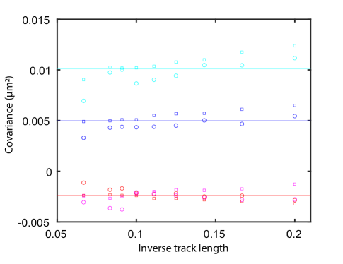
Table 2 reports the mean covariances, and , the mean diffusivity, and the mean localization noise for these two diffusive states, as well as the fraction of the population corresponding to state 1, , the fraction of the population corresponding to state 2, . Evidently, pEMv2 indicates the existence of a relatively low diffusivity state (state 1) with m2s-1 and a relatively high diffusivity state (state 2) with m2s-1, for a track length of 9 steps. Both states have roughly equal representation in the overall population with and .
Table 2 reveals that the diffusivity of state 2, returned by pEMv2, decreases as the track length increases. We hypothesize that this circumstance arises because for increasing track length, high diffusivity tracks have a progressively higher probability to diffuse out of the illuminated volume than lower diffusivity tracks. Thus, a population of longer tracks is preferentially depleted of high-diffusivity tracks, pulling down the population’s mean diffusivity, compared to a population of shorter tracks.
4.5 Mean-square displacements (MSDs) versus delay time of pEMv2-sorted trajectories
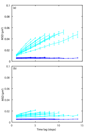
In Sec. 4.4, we used the pEMv2-determined mean covariances to estimate the diffusivity of each diffusive state. Ref. Vestergaard2014 showed that such covariance-based estimators are statistically optimal. However, another widely-used means of characterizing diffusivity is via the slope of the mean-square displacement (MSD) versus time delay, which is a linear function for simple diffusion. Fig. 6(a) plots the mean-square MSDs for TRAP-labeled Pma1 trajectories for each state versus the number of steps. The MSDs for tracks corresponding to state 1 are shown in blue, while the MSDs for tracks corresponding to state 2 are shown in cyan. Evidently, the MSDs for state 1 are conspicuously constant versus time. This observation emphasizes that state 1 really is essentially immobile. By contrast, it is clear that the state-2 MSDs increase approximately linearly versus time, consistent with what is expected for simple diffusion. It is also apparent that the slopes of the state-2 MSDs tend to decrease with increasing track length, corresponding to an apparently decreasing diffusivity with increasing track length, mirroring the behavior observed for the covariance-based estimates of the diffusivity.
4.6 Covariance distributions of pEMv2-sorted TRAP-labeled Pma1 trajectories agree with theory
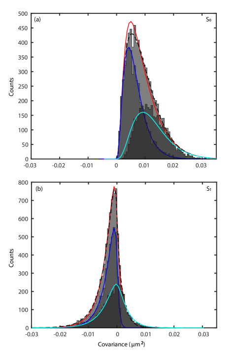
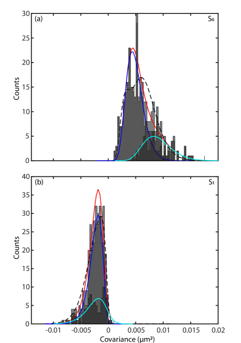
To further assess the performance of pEMv2, we first sought to compare the theoretical covariance distributions for each state, conditioned on their respective experimental mean covariances, and , to the corresponding experimental distributions. Such comparisons are presented in Fig. 7, Fig. 8, and Fig. 9, which plot both experimental and theoretical covariance distributions for 5-step, 9-step, and 15-step trajectories, respectively, sorted into states 1 and 2 and for the overall population of unsorted trajectories. Stepped histograms represent the experimental covariance distributions. Smooth lines are the theoretical covariance distributions with blue and cyan corresponding to the distributions (Eq. 4) for state 1 and state 2, respectively, and red corresponding to the two-component distribution (Eq. 11) for the overall, unsorted population. In all cases,the theory and experiment appear to be in good agreement, despite the fact that no fitting is involved: The only input for the theoretical curves in these figures are the experimental mean values of and . The fact that the distributions to emerge from the pEMv2-sorted populations agree well with what is expected theoretically, without any fitting, strongly supports that pEMv2 is correctly characterizing the diffusive behavior of TRAP-labeled Pma1. Quantitative comparisons of the pEMv2-sorted experimental distributions and theory using the Kolmogorov-Smirnov test are described in Supplementary Material 1A.
4.7 pEMv2 finds two diffusive states for Pma1-mEos3.2 direct-fusion trajectories
Next, we applied pEMv2 and the theory of Sec. 2.3 to Pma1-mEos3.2 direct-fusion trajectories. As shown in Fig. 11, for track lengths of 5, 6, 7, 8, 9, 10, 11, 12, and 15, the BIC was maximized for two states. However, the increase in the BIC, going from one state to two states, is much less in this case (), than for TRAP-labeled Pma1 trajectories (, Fig. 5), indicating that pEMv2’s preference for a two state description over a one-state description is much less for Pma1-mEos3.2 than for TRAP-labeled Pma1.
| Track Length | ||||||||||||||||||
|---|---|---|---|---|---|---|---|---|---|---|---|---|---|---|---|---|---|---|
| 5 | 0.0056 | 4.65 | -0.0029 | 4.19 | -0.0021 | 0.0013 | 0.0028 | 3.47 | 0.0128 | 1.64 | -0.0048 | 1.78 | 0.081 | 0.0063 | 0.0053 | 1.41 | 0.84 | 0.16 |
| 6 | 0.0058 | 5.17 | -0.0029 | 4.27 | 0.0012 | 0.0012 | 0.0029 | 3.61 | 0.0123 | 2.00 | -0.0046 | 2.08 | 0.079 | 0.0071 | 0.0051 | 1.673 | 0.89 | 0.11 |
| 7 | 0.0053 | 5.03 | -0.0027 | 4.26 | 0.00075 | 0.0013 | 0.0027 | 3.57 | 0.0111 | 1.57 | -0.0047 | 1.56 | 0.0448 | 0.0053 | 0.0050 | 1.26 | 0.82 | 0.18 |
| 8 | 0.0057 | 5.76 | -0.0028 | 4.56 | 0.0021 | 0.0013 | 0.0028 | 3.89 | 0.0115 | 2.40 | -0.0045 | 2.32 | 0.061 | 0.0075 | 0.0049 | 1.90 | 0.91 | 0.09 |
| 9 | 0.0055 | 5.98 | -0.0027 | 4.72 | 0.0015 | 0.0013 | 0.0027 | 4.03 | 0.0107 | 2.14 | -0.0046 | 2.10 | 0.040 | 0.0068 | 0.0048 | 1.70 | 0.89 | 0.11 |
| 10 | 0.0054 | 6.18 | -0.0026 | 4.82 | 0.0032 | 0.0014 | 0.0027 | 4.13 | 0.0102 | 2.37 | -0.0044 | 2.16 | 0.035 | 0.0066 | 0.0046 | 1.79 | 0.89 | 0.11 |
| 11 | 0.0053 | 6.30 | -0.0026 | 4.81 | 0.0020 | 0.0013 | 0.0026 | 4.14 | 0.0100 | 2.32 | -0.0042 | 2.05 | 0.032 | 0.0064 | 0.0044 | 1.70 | 0.86 | 0.14 |
| 12 | 0.0049 | 5.90 | -0.0024 | 4.41 | 0.0036 | 0.0013 | 0.0024 | 3.80 | 0.0090 | 1.64 | -0.0042 | 1.45 | 0.0136 | 0.0045 | 0.0043 | 1.20 | 0.77 | 0.23 |
| 15 | 0.0050 | 6.80 | -0.0025 | 5.16 | 0.0012 | 0.0014 | 0.0025 | 4.45 | 0.0087 | 2.01 | -0.0040 | 1.80 | 0.0166 | 0.00549 | 0.0041 | 1.50 | 0.82 | 0.18 |
Table 3 reports the mean covariances, and , the mean diffusivity, and the mean localization noise for the two diffusive states, found in this case, as well as the fraction of the population corresponding to state 1, , the fraction of the population corresponding to state 2, . From this table, it is clear that pEMv2 finds that Pma1-mEos3.2 is overall significantly less mobile than TRAP-labeled Pma1. First, the immobile state (state 1) constitutes about 90% of the total population. Second, the diffusivity of the higher diffusivity state (state 2) is just m2s-1, several times smaller than the diffusivity of TRAP-labeled Pma1’s higher-diffusivity state, for which m2s-1. Hence, the more-mobile second state in this labeling method, is still far less mobile than the mobile state for the indirect labeling.
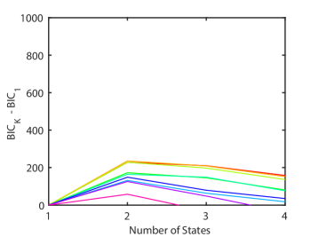
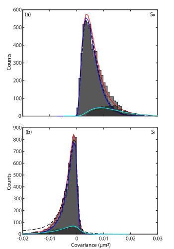
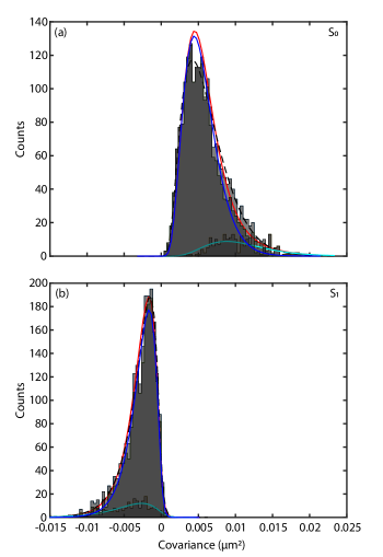
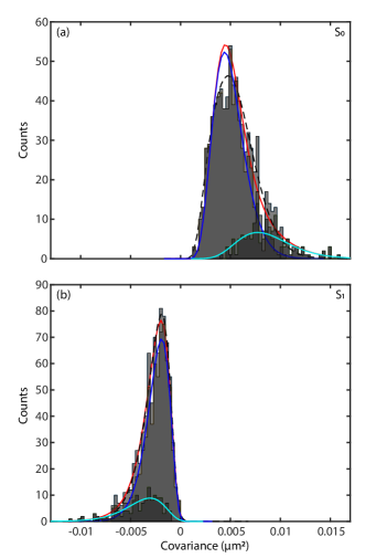
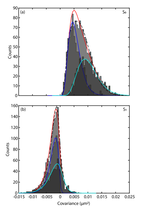
Fig. 12, Fig. 13 , and Fig. 14 compare the experimental covariance distributions for Pma1-mEos3.2 trajectories with track lengths of 5, 9, and 15 steps, respectively, to the corresponding theoretical predictions. In each figure, there appears to be good agreement between theory and data, even though no fitting is involved. The fact that the distributions to emerge from the pEMv2-sorted populations agree well with what is expected theoretically supports that pEMv2 is correctly characterizing the diffusive behavior of Pma1-mEOs3.2. Quantitative comparisons of the pEMv2-sorted experimental distributions and theory, using the Kolmogorov-Smirnov test, are described in Supplementary Material 1B.
Fig. 4(b) shows the diffusivity distributions for Pma1-mEOs3.2 trajectories. Two features stand out from this figure in comparison to Fig. 4(a). First, the population fraction of the higher diffusivity state (state 2) is significantly less for the direct fusion than for TRAP-labeled Pma1. Second, the mean diffusivity of the higher diffusivity state (state 2) is significantly less for the direct fusion (m2s-1)than for TRAP-labeled Pma1 (m2s-1). These two features make the overall diffusivity of Pma1-mEos3.2 significantly smaller than that of TRAP-labeled Pma1.
5 Conclusion
Two primary conclusions are to be drawn from this work. First, the diffusive behavior of Pma1 can be described convincingly in terms of two discrete diffusive states, each with its own diffusive properties, sorted by the pEMv2 software, and validated using our theoretical covariance distributions. Specifically, we investigated two differently labeled versions of Pma1 at the single molecule level using single particle tracking under TIRF illumination. Using a machine-learning-based approach that identifies and sorts a population of trajectories into a discrete number of diffusive states, pEMv2, we found that a minimally-modified version of Pma1, with a C-terminal five-amino-acid tag that reversibly binds to a TRAP-mEos3.2 fusion, shows comparable population fractions of a mobile state, corresponding to simple diffusion with a diffusion constant consistent with what is expected for a membrane protein, and an essentially immobile state. By contrast, we found that a Pma1-mEos3.2 direct fusion is overwhelmingly in an immobile state, and the small population fraction, assigned to a more mobile state by pEMv2, has a diffusion coefficient several times smaller than the diffusion coefficient of mobile TRAP-labeled Pma1. A comparison between the experimental pEMv2-sorted covariance and diffusivity distributions, conditioned on the experimental mean covariances of the sorted tracks, and the corresponding theoretical distributions that we derived, shows overall good agreement without any fitting, providing strong support for pEMv2-based sorting. Additionally, we note that the method used to label a protein for microscopy visualization in living cells can affect the protein’s diffusive behavior in a substantial fashion with unknown consequences for its biological function. Further studies are required to determine which labeling method more closely represents the motion of the unlabeled protein. Second, we found that both variants of Pma1 studied in this work, TRAP-labeled Pma1 and Pma1-mEos3.2, are monomers in vivo. This result is noteworthy because in vitro preparations for electron microscopy show Pma1 forms hexamers. We estimated the lifetime of the TRAP-peptide bound-state to be 0.15 s. An open question remains as to whether Pma1’s two diffusive states are significant for Pma1’s biological function, and if so what their roles might be.
Acknowledgments M.L.P.B. and S.E.P. contributed equally to this work. M.L.P.B. conceived the project, analyzed data, and wrote the paper; S.E.P. conceived the project, collected data, analyzed data, and wrote the paper; Y.Z. conceived the project, collected data, and wrote the paper; M.H. conceived the project, constructed the yeast strains, and wrote the paper; J.B. conceived the project and wrote the paper; L.R. conceived the project and wrote the paper; S.G.J.M. conceived the project and wrote the paper. This research was supported by the National Institutes of Health via NIH R01 GM118528 and NIH P30 DK045735. M.L.P.B. was supported by NIH T32EB019941 and the NSF GRFP. S.E.P. was supported by the NSF GRFP and NSF PHYS 1522467. J. B. discloses significant financial interest in Bruker Corp., Hamamatsu Photonics, and Panluminate Inc.
References
- \bibcommenthead
- (1) R.W. Albers, Biochemical aspects of active transport. Annual Review of Biochemistry 36(1), 727–756 (1967). 10.1146/annurev.bi.36.070167.003455
- (2) R.L. Post, C. Hegyvary, S. Kume, Activation by adenosine triphosphate in the phosphorylation kinetics of sodium and potassium ion transport adenosine triphosphatase. Journal of Biological Chemistry 247(20), 6530–6540 (1972). 10.1016/s0021-9258(19)44725-x
- (3) E. Goormaghtigh, C. Chadwick, G.A. Scarborough, Monomers of the neurospora plasma membrane H+-ATPase catalyze efficient proton translocation. J. Biol. Chem. 261, 7466–7471 (1986)
- (4) P. Morsomme, C.W. Slayman, A. Goffeau, Mutagenic study of the structure, function and biogenesis of the yeast plasma membrane H+-atpase. Biochimica et Biophysica Acta (BBA) - Reviews on Biomembranes 1469(3), 133–157 (2000). 10.1016/s0304-4157(00)00015-0
- (5) K. Malínská, J. Malínský, M. Opekarová, W. Tanner, Visualization of protein compartmentation within the plasma membrane of living yeast cells. Molecular Biology of the Cell 14(11), 4427–4436 (2003). 10.1091/mbc.e03-04-0221
- (6) W. Kühlbrandt, Biology, structure and mechanism of p-type ATPases. Nature Reviews Molecular Cell Biology 5(4), 282–295 (2004). 10.1038/nrm1354
- (7) F. Spira, N.S. Mueller, G. Beck, P. von Olshausen, J. Beig, R. Wedlich-Soeldner, Patchwork organization of the yeast plasma membrane into numerous coexisting domains. Nature Cell Biology 14, 640–648 (2012)
- (8) A. Mason, C. Slayman, in Encyclopedia of Biological Chemistry (Elsevier, 2013), pp. 688–692. 10.1016/b978-0-12-378630-2.00194-8
- (9) K.A. Henderson, A.L. Hughes, D.E. Gottschling, Mother-daughter asymmetry of pH underlies aging and rejuvenation in yeast. eLife 3 (2014). 10.7554/elife.03504
- (10) A. Athanasopoulos, B. Andre, V. Sophianopoulou, C. Gournas, Fungal plasma membrane domains. FEMS Microbiology Reviews 43, 642–673 (2019)
- (11) S. Heit, M.M.G. Geurts, B.J. Murphy, R.A. Corey, D.J. Mills, W. Kühlbrandt, M. Bublitz, Structure of the hexameric fungal plasma membrane proton pump in its autoinhibited state. Science Advances 7(46), eabj5255 (2021). 10.1126/sciadv.abj5255. URL https://www.science.org/doi/abs/10.1126/sciadv.abj5255
- (12) P. Zhao, C. Zhao, D. Chen, C. Yun, L. Bai, Structure and activation mechanism of the hexameric plasma membrane H+-ATPase. Nat. Commun. 12, 6439 (2021)
- (13) S.E. Pratt, E.B. Speltz, S.G.J. Mochrie, L. Regan, Designed proteins as novel imaging reagents in LivingEscherichia coli. ChemBioChem 17(17), 1652–1657 (2016). 10.1002/cbic.201600252
- (14) C. Oi, Z. Gidden, L. Holyoake, O. Kantelberg, S. Mochrie, M.H. Horrocks, L. Regan, A step-by-step protocol for performing LIVE-PAINT super-resolution imaging of proteins in live cells using reversible peptide-protein interactions (2020). 10.21203/rs.3.pex-1043/v1
- (15) M. Hinrichsen, M. Lenz, J.M. Edwards, O.K. Miller, S.G.J. Mochrie, P.S. Swain, U. Schwarz-Linek, L. Regan, A new method for post-translationally labeling proteins in live cells for fluorescence imaging and tracking. Protein Engineering, Design and Selection 30(12), 771–780 (2017). 10.1093/protein/gzx059
- (16) C. Oi, Z. Gidden, L. Holyoake, O. Kantelberg, S. Mochrie, M.H. Horrocks, L. Regan, LIVE-PAINT allows super-resolution microscopy inside living cells using reversible peptide-protein interactions. Communications Biology 3(1) (2020). 10.1038/s42003-020-01188-6
- (17) C. Oi, S.G.J. Mochrie, M.H. Horrocks, L. Regan, PAINT using proteins: A new brush for super-resolution artists. Protein Science 29(11), 2142–2149 (2020). 10.1002/pro.3953
- (18) W.K. Huh, J.V. Falvo, L.C. Gerke, A.S. Carroll, R.W. Howson, J.S. Weissman, E.K. O’Shea, Global analysis of protein localization in budding yeast. Nature 425(6959), 686–691 (2003). 10.1038/nature02026
- (19) D.L. Coutu, T. Schroeder, Probing cellular processes by long-term live imaging – historic problems and current solutions. Journal of Cell Science (2013). 10.1242/jcs.118349
- (20) C. Li, A. Tebo, A. Gautier, Fluorogenic labeling strategies for biological imaging. International Journal of Molecular Sciences 18(7), 1473 (2017). 10.3390/ijms18071473
- (21) C.P. Toseland, Fluorescent labeling and modification of proteins. Journal of Chemical Biology 6(3), 85–95 (2013). 10.1007/s12154-013-0094-5
- (22) E.C. Jensen, Use of fluorescent probes: Their effect on cell biology and limitations. The Anatomical Record: Advances in Integrative Anatomy and Evolutionary Biology 295(12), 2031–2036 (2012). 10.1002/ar.22602
- (23) F. Montecinos-Franjola, B.L. Bauer, J.A. Mears, R. Ramachandran, GFP fluorescence tagging alters dynamin-related protein 1 oligomerization dynamics and creates disassembly-refractory puncta to mediate mitochondrial fission. Scientific Reports 10(1) (2020). 10.1038/s41598-020-71655-x
- (24) C.S. Lisenbee, S.K. Karnik, R.N. Trelease, Overexpression and mislocalization of a tail-anchored gfp redefines the identity of peroxisomal er. Traffic 4(7), 491–501 (2003). 10.1034/j.1600-0854.2003.00107.x
- (25) M.L.P. Bailey, H. Yan, I. Surovtsev, J.F. Williams, M.C. King, S.G.J. Mochrie, Covariance distributions in single particle tracking. Physical Review E 103(3) (2021). 10.1103/physreve.103.032405
- (26) P.K. Koo, M. Weitzman, C.R. Sabanaygam, K.L. van Golen, S.G. Mochrie, Extracting diffusive states of Rho GTPase in live cells: towards in vivo biochemistry. PLoS Computational Biology 11(10) (2015)
- (27) P.K. Koo, S.G. Mochrie, Systems-level approach to uncovering diffusive states and their transitions from single-particle trajectories. Physical Review E 94(5), 052,412 (2016)
- (28) I. Rey-Suarez, B.A. Wheatley, P. Koo, A. Bhanja, Z. Shu, S. Mochrie, W. Song, H. Shroff, A. Upadhyaya, WASP family proteins regulate the mobility of the b cell receptor during signaling activation. Nature Communications 11(1) (2020). 10.1038/s41467-020-14335-8
- (29) C.L. Vestergaard, P.C. Blainey, H. Flyvbjerg, Optimal estimation of diffusion coefficients from single-particle trajectories. Physical Review E 89(2), 022,726 (2014)
- (30) B. Justesen, R. Hansen, H. Martens, L. Theorin, M. Palmgren, K. Martinez, T. Pomorski, A. Fuglsang, Active plasma membrane p-type H+-ATPase reconstituted into nanodiscs is a monomer. J. Biol. Chem. pp. 26,419–26,429 (2013)
- (31) M. Saxton, Single-particle tracking: the distribution of diffusion coefficients. Biophysical Journal 72(4), 1744–1753 (1997). 10.1016/s0006-3495(97)78820-9
- (32) T. Savin, P.S. Doyle, Statistical and sampling issues when using multiple particle tracking. Physical Review E 76(2) (2007). 10.1103/physreve.76.021501
- (33) N. Monnier, Z. Barry, H.Y. Park, K.C. Su, Z. Katz, B.P. English, A. Dey, K. Pan, I.M. Cheeseman, R.H. Singer, M. Bathe, Inferring transient particle transport dynamics in live cells. Nature Methods 12(9), 838–840 (2015). 10.1038/nmeth.3483
- (34) R. Das, C.W. Cairo, D. Coombs, A hidden markov model for single particle tracks quantifies dynamic interactions between LFA-1 and the actin cytoskeleton. PLoS Computational Biology 5(11), e1000,556 (2009). 10.1371/journal.pcbi.1000556
- (35) P.J. Slator, C.W. Cairo, N.J. Burroughs, Detection of diffusion heterogeneity in single particle tracking trajectories using a hidden markov model with measurement noise propagation. PLOS ONE 10(10), e0140,759 (2015). 10.1371/journal.pone.0140759
- (36) R. Zhao, J. Yuan, N. Li, Y. Sun, T. Xia, X. Fang, Analysis of the diffusivity change from single-molecule trajectories on living cells. Analytical Chemistry 91(21), 13,390–13,397 (2019). 10.1021/acs.analchem.9b01005
- (37) H.D. Pinholt, S.S.R. Bohr, J.F. Iversen, W. Boomsma, N.S. Hatzakis, Single-particle diffusional fingerprinting: A machine-learning framework for quantitative analysis of heterogeneous diffusion. Proceedings of the National Academy of Sciences 118(31), e2104624,118 (2021). 10.1073/pnas.2104624118
- (38) M. Hinrichsen, Applying protein-peptide interactions to fluorescently label proteins in s. cerevisiae. Ph.D. thesis, Yale University (2018)
- (39) Y. Zhang, M. Lara-Tejero, J. Bewersdorf, J.E. Galán, Visualization and characterization of individual type III protein secretion machines in live bacteria. Proceedings of the National Academy of Sciences 114(23), 6098–6103 (2017). 10.1073/pnas.1705823114
- (40) J.C. Crocker, D.G. Grier, Methods of digital video microscopy for colloidal studies. Journal of Colloid and Interface Science 179(1), 298–310 (1996)
- (41) C. Oi, Reversible peptide-protein interactions inside cells: Enabling a new approach for achieving super-resolution imaging in live cells. Ph.D. thesis, Yale University (2021)