Poncelet Spatio-Temporal Surfaces and Tangles

Abstract

We explore geometric properties of 3d surfaces swept by a family of Poncelet triangles, as well as tangles produced by space curves they define.

1   Introduction

Depicted in Figure 1(left) is Poncelet’s closure theorem in the special case of triangles. The theorem states that two conics $\mathcal{E}$ and $\mathcal{E}^{\prime}$ are chosen so that a polygon can be drawn with all vertices on $\mathcal{E}$ and all sides tangent to $\mathcal{E}^{\prime}$, then a porism of such polygons exists: any point $P$ on $\mathcal{E}$ can be used as an initial vertex for a polygon with identical incidence/tangency properties with respect to $\mathcal{E},\mathcal{E}^{\prime}$. For more details, see [5, 6, 7].

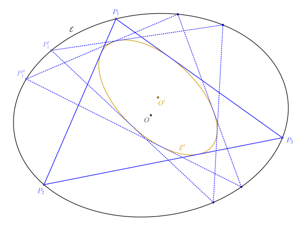
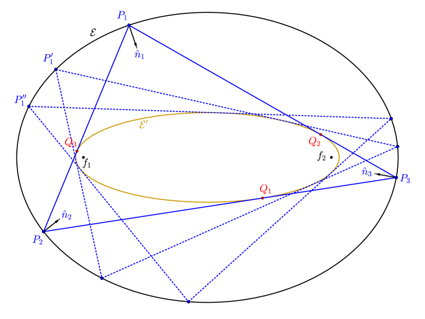
Figure 1: Left: Poncelet’s closure theorem for triangles. Right: Ellipses $\mathcal{E},\mathcal{E}^{\prime}$ are confocal. Consecutive sides of the Poncelet family (blue) are bisected by the normals $\hat{n}_{i}$, and the perimeter is constant. Also shown are the three points of contact $Q_{i}$ with the inner ellipse, or caustic.

 

Referring to Figure 1(right), a property-rich choice for $\mathcal{E},\mathcal{E}^{\prime}$ is when they are confocal ellipses, i.e., with shared foci. If such a pair admits a Poncelet porism, two immediate consequences ensue: (i) consecutive sides are bisected by the normal to $\mathcal{E}$ and Poncelet polygons can therefore be regarded as the periodic path of a particle bouncing elastically against $\mathcal{E}$ (this is known as the “elliptic billiard”, see [16]), and (ii) all polygons in the porism have the same perimeter [16]. Dozens of other properties and invariants can be derived from these an interesting one being constant sum of the internal angle cosines, proved in [1, 4]. For more properties of the confocal family, see [10, 12].

Summary:

in Section 2 we define a ruled surface based on Poncelet triangles, and discuss properties of its curvature. In Section 3 we study the link topology of space curves swept by points of contact, and triangle centers. In Section 4, we list several unexplored experimental alternatives. To facilitate reproducibility, in Appendices A and B we include explicit expressions for both the Poncelet triangle parametrization and Gaussian and mean curvature. The pages listed in Table 1 allow for live interaction with some objects mentioned herein.

title	http://observablehq.com/<.>
PSTS Visualization (live)	@esperanc/3-periodic-elliptical-billiards-3d-sweep	go
PSTS Visualization (static)	@dan-reznik/elliptic-billiard-triangle	go
Poncelet’s Closure Theorem	@dan-reznik/poncelet-iteration	go
Jacobi’s Elliptic Functions	@dan-reznik/jacobi-elliptic-functions	go

Table 1: Pages with interactive simulations to the various phenomena mentioned in the article.

2   A Poncelet Spatio-Temporal Surface (PSTS)

To achieve a homogeneous traversal of the Poncelet family, we parametrize it with Jacobi elliptic functions, as explained in Appendix A. Let $u$ be its parameter, $u\in[0,T]$, where $T$ is the period. Let $P_{i}(u)$ be a vertex of the family and $Q_{i}(u,v)$ be a point on edge $P_{i}(u)P_{i+1}(u)$, namely, $Q_{i}(u,v)=(1-v)P_{i}(u)+vP_{i+1}(u)$, $v\in[0,1]$. Referring to Figure 2(left):

Definition 1.

The Poncelet Spatio-Temporal Surface $\mathcal{S}$ (SPTS) is the union of the 3 parametric ruled surfaces $\mathcal{S}_{i}=[u,Q_{i}(u,v)]$, $i=1,2,3$. Note that the $u$ parameter is periodic.

Recall that the Gaussian $\mathcal{K}$ (resp. mean $\mathcal{H}$) curvature) of a surface is the product (resp. average) of its principal curvatures, see [14]. Referring to Figure 2(right), and using the expressions in Appendix B, we have derived rather long analytic expressions for both curvatures. Laborious analysis reveals that:

Proposition 1.

The three facets $\mathcal{S}_{i}$ of $\mathcal{S}$ are hyperbolic, i.e., each has negative Gaussian curvature everywhere.

Consider one facet $\mathcal{S}_{1}$ of $\mathcal{S}$. Let $Q_{1}=(0,1/2)$, $Q_{2}=(T/4,1/2)$, $Q_{3}=(T/2,1/2)$, $Q_{4}=(3T/4,1/2)$. These four points correspond to the isosceles configurations shown in Figure 4(right). Referring to Figure 5:

Proposition 2.

$Q_{1}$ and $Q_{3}$ (resp. $Q_{2}$ and $Q_{4}$) are non degenerate (Morse type) local minima (resp. saddlepoints) of $\mathcal{H}$. Conversely, $Q_{2}$ and $Q_{4}$ (resp. $Q_{1}$ and $Q_{3}$) are non degenerate (Morse type) local minima (resp. saddlepoints) of $\mathcal{K}$.

Analogous statements can be made for facets $S_{2}$ and $S_{3}$. It is worth noting that in general the critical points of Gaussian and Mean curvatures do not coincide. We currently think this is a feature of any Poncelet triangle family defined between a pair of concentric, axis-aligned ellipses.

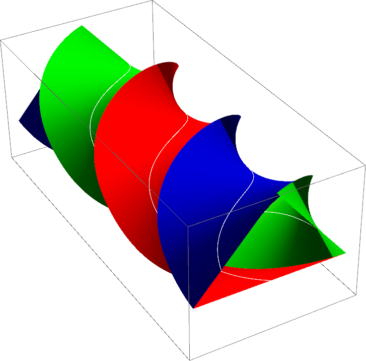
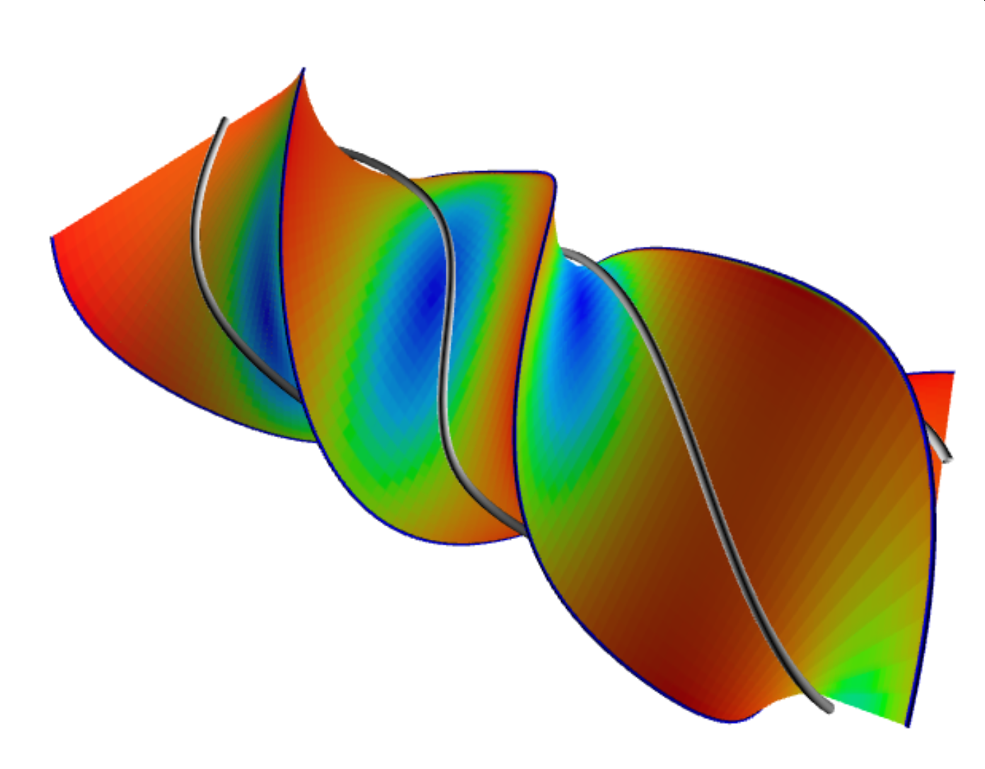
Figure 2: Left: the PSTS swept by Poncelet triangles in the confocal family. It is a union of three ruled surfaces (red, green, and blue), each of which has negative curvature. Also shown is the 3d curve swept by the points of contact $Q_{i}$ (white). Right: the SPTS colored by Gaussian curvature. The center of the blue areas represent minima.

 

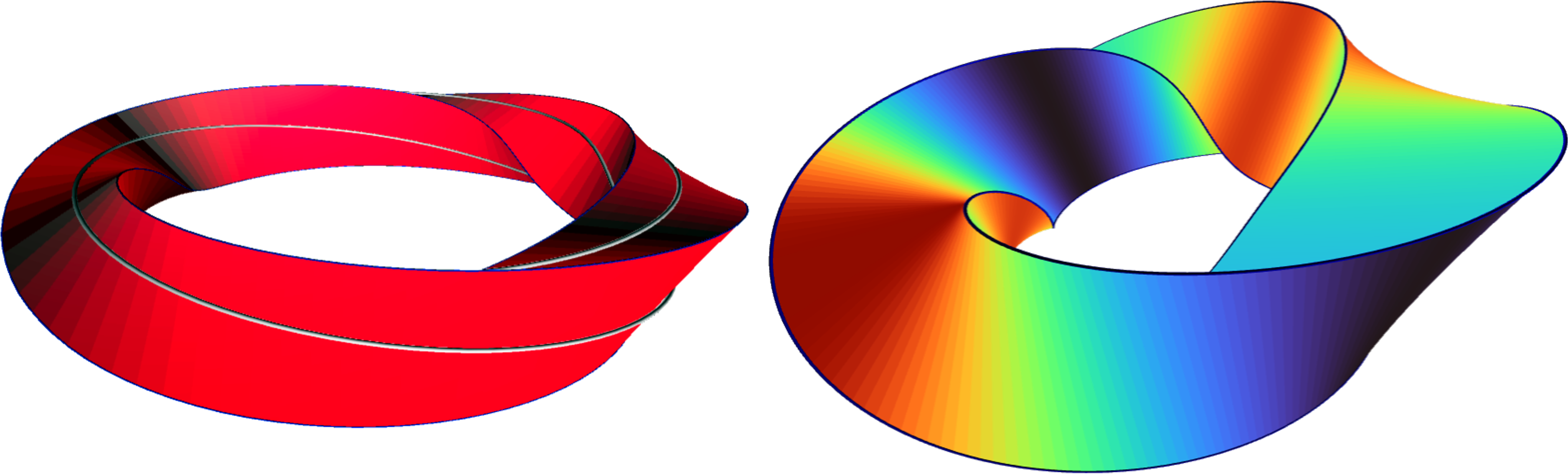
Figure 3: Left: identifying the $u=0$ with $u=T$ cross-sections of the PSTS, obtain an orientable Seifert surface [17]. Also shown is the path of the contact points (white) with the caustic. Right: The same surface now colored by the torsion of straight lines elements sweeping the surface. Logo applications accepted.

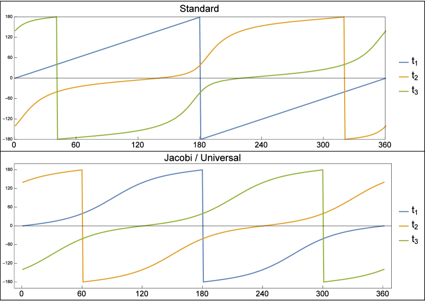
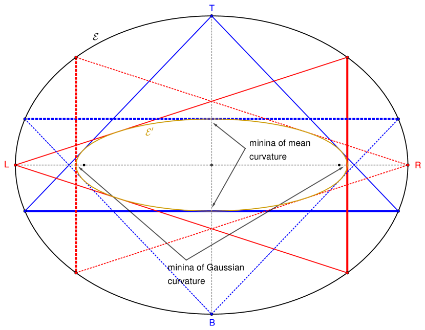
Figure 4: Left top: under the “standard parametrization” $P_{1}(t)=[a\cos{t},b\sin{t}]$ the angular position of vertices of Poncelet triangles in the confocal pair are three different curves. Left bottom: under Jacobi’s parametrization, the curves become 120-degree delayed copies of one another. Right: The confocal family has four isosceles triangles, with a vertex on either the top (T), bottom (B), left (L) or right (R) vertices of the outer ellipse $\mathcal{E}$. The Gaussian (resp. mean) curvature of the spatio-temporal surface have minima when its cross section is one of said isosceles triangles. The critical point occurs at the midpoint of the base (thick segment) when the apex is on L or R (resp. T or B).

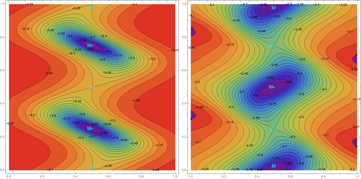
Figure 5: Left: Gaussian curvature of Jacobi-parametrized Poncelet triangles in the confocal family (horizontal is the position along a given side, and vertical is one revolution of the family. Points $M$ (resp. $S$) denote the curvature minima (saddle points). Right: The mean curvature, with $M,S$ as before.

3   Space Curve Tangles

Consider the surface obtained by identifying the $u=0$ and $u=T$ cross sections of $\mathcal{S}$, shown in Figure 3. Each contact point $Q_{i}$ of Figure 1(right) will sweep a wiggly ring; their union will form a tangle known as a 3-link of “Hopf” rings [2, 13], distinct from the Borromean tangle, see Figure 6. Indeed, the same tangle is swept by the 3 vertices of the family, and it is independent of the family being a Poncelet one. The surface whose boundary is a 3-link tangle is a type of Seifert surface [17].

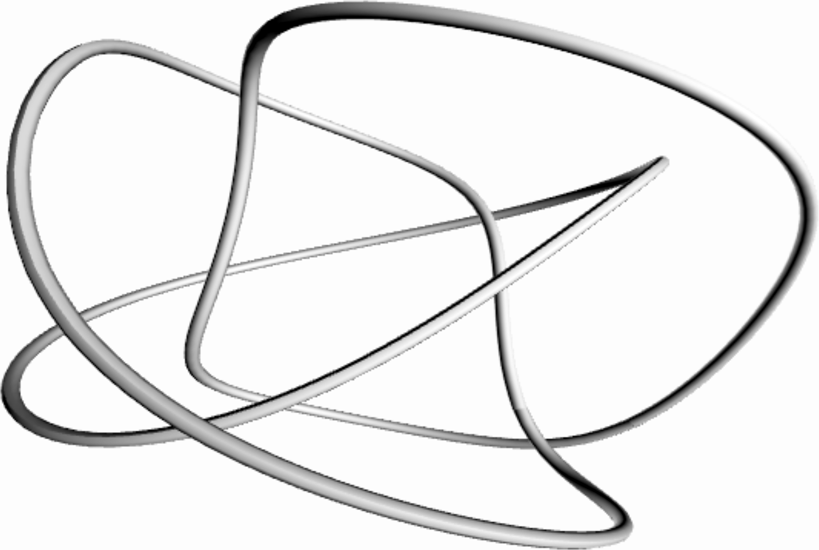
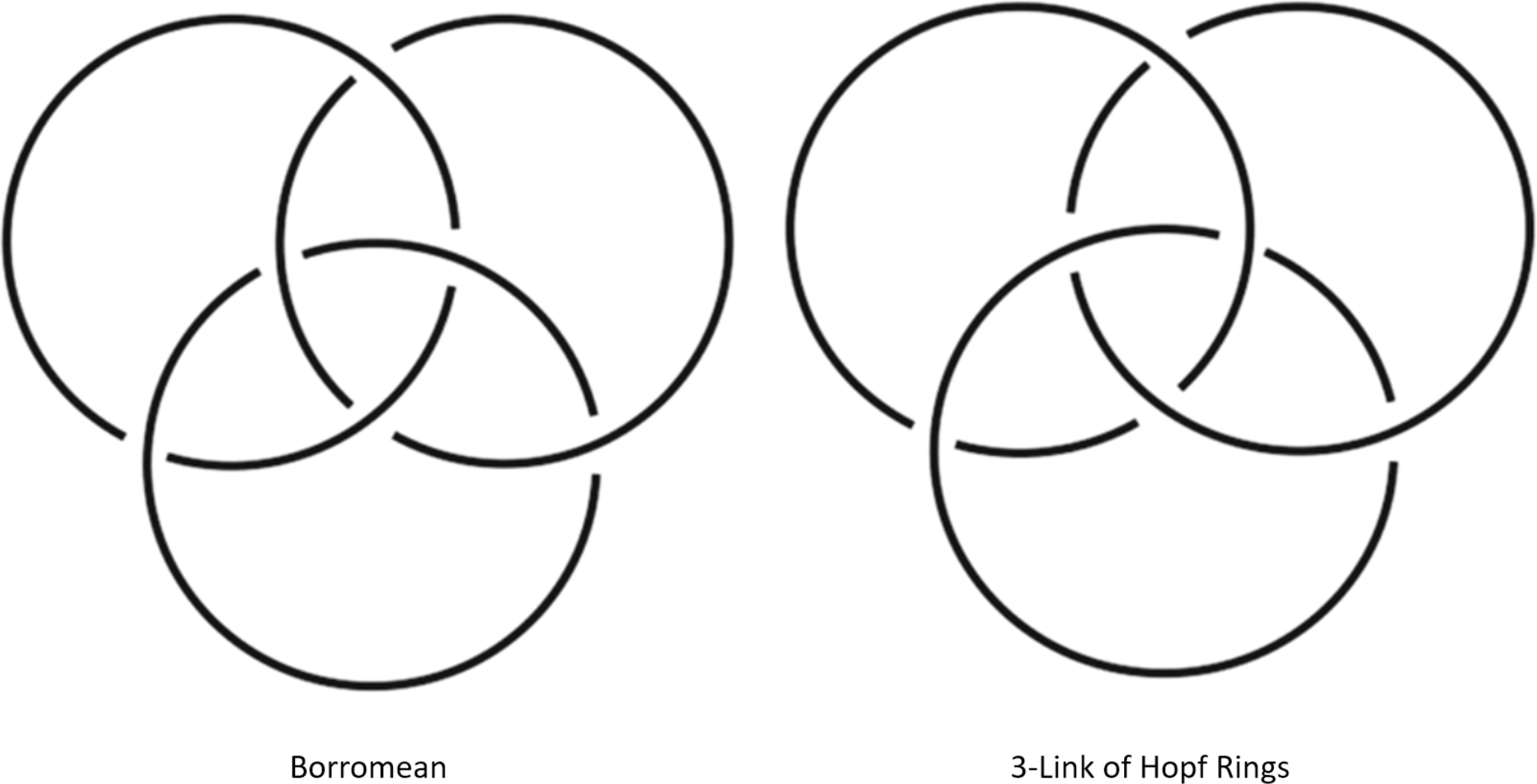
Figure 6: Left: The contact points of the identified PSTS sweep a triad of “Hopf” rings forming a 3-link tangle [2]. Right: Two type of 3-ring tangles: Borromean (left), and the Hopf 3-link (right) [2], homeomorphic to the curves swept by the contact points. Note that by removing one of the rings in the former (resp. latter) case, the other two are free (resp. remain tangled).

 

Referring to Figure 7, more tangle topologies are obtained if one also considers the relative motion of notable points of the triangle (e.g., the incenter, the barycenter, etc.) over the Poncelet family. See [11] for 2d analysis of such loci.

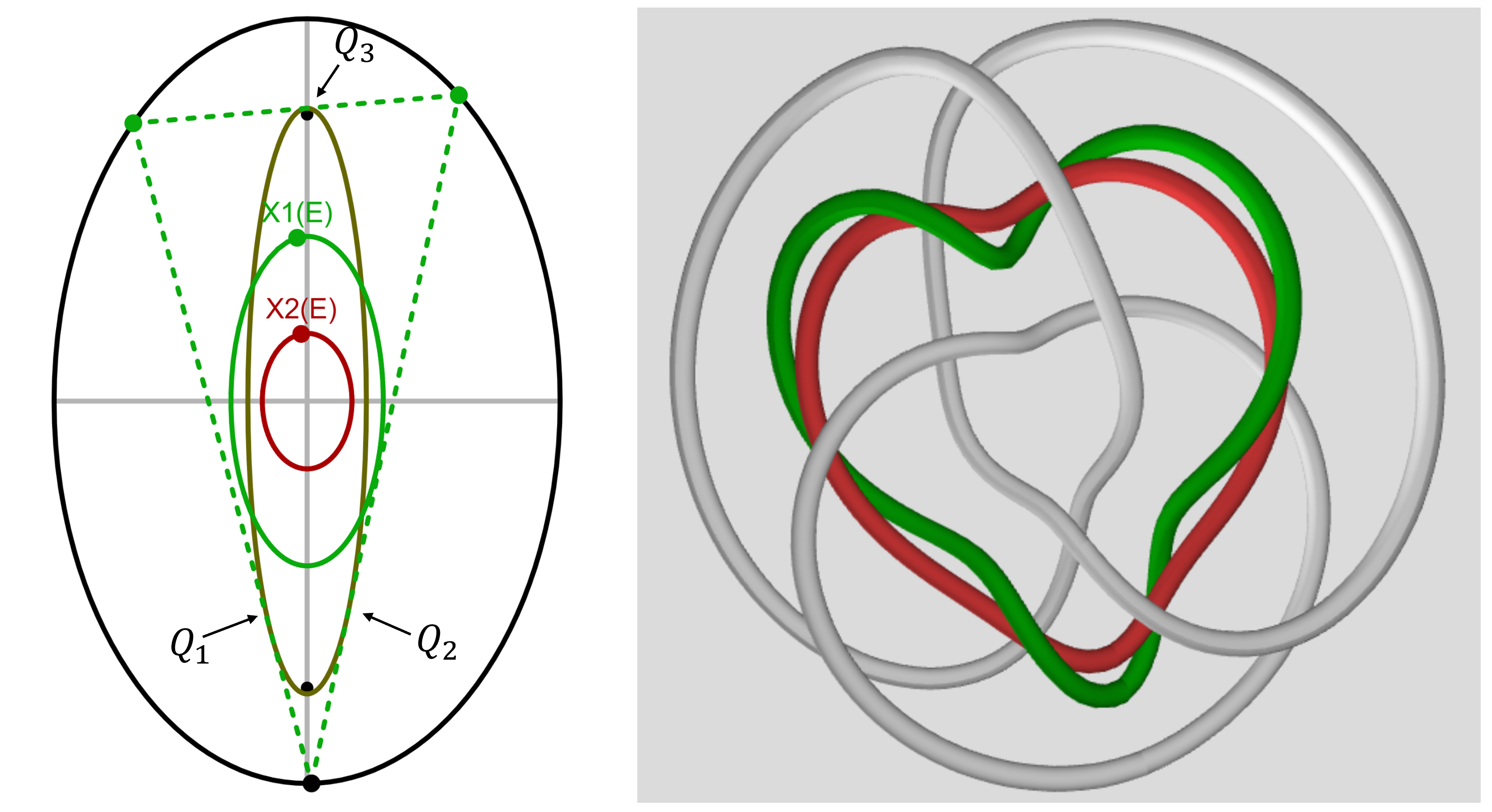
Figure 7: Left: the confocal family (rotated $90^{o}$), and the locus of the incenter $X_{1}$ (green) and barycenter $X_{2}$ (red). Also shown are the three contact points $Q_{i}$ with the caustic. Right: In the endpoint-identified PSTS, the space curves swept by $X_{1}$ (green) forms an individual a 2-link tangle with each individual contact point ring (gray). The same is true for the $X_{2}$ space curve (red). $X_{1}$ and $X_{2}$ form a link thrice twisted about each other.

4   Next Steps

To continue this exploration one could consider:

1. Different Poncelet families, see examples in Figure 8;

2. Picking a hyperbola or parabola for either $\mathcal{E},\mathcal{E}^{\prime}$, e.g., as in this video;

3. Non-closing Poncelet polylines Figure 9(left);

4. Poncelet $N$-gons, $N>3$, including self-intersected ones as in Figure 9(right). See [9].

5. Families of derived triangles, e.g., the excentral, orthic, medial triangles [18]

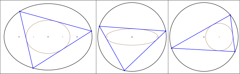
Figure 8: From left to right, three additional examples of Poncelet triangle families in (i) a homothetic pair of ellipses, (ii) inscribed in a circle and circumscribing a concentric ellipse, and (iii) interscribed between two non-concentric circles (aka., the “bicentric” pair). Video

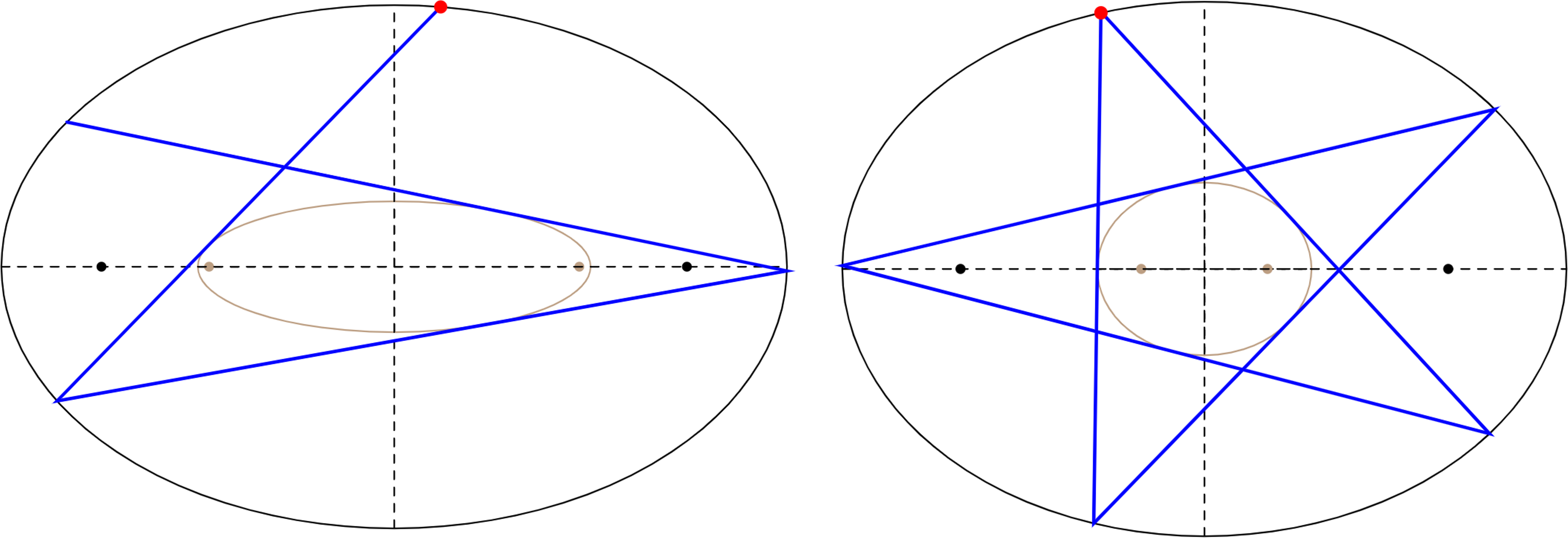
Figure 9: Left: a non-closing Poncelet 3-polyline. Right: a self-intersected $N=5$ Poncelet family (pentagrams).

Appendix A Jacobi Parametrization

We parametrize Poncelet triangles using Jacobi elliptic functions since an application of the Poncelet map corresponds to a unit translations in the argument of said functions. As seen in Figure 4(left), this entails that the angular position of vertices are identical, time-delayed functions.

Following the notation in [3], $k\in[0,1]$ denote the elliptic modulus:

Definition 2.

The incomplete elliptic integral of the first kind $K(\varphi,k)$ is given by:

$$K(\varphi,k)=\int_{0}^{\varphi}\frac{d\theta}{\sqrt{1-k^{2}\sin^{2}\theta}}$$ (1)

The complete elliptic integral of the first kind $K(k)$ is simply $K(\pi/2,k)$.

Definition 3.

The elliptic sine sn, cosine cn, and delta-amplitude dn are given by:

$$\text{sn}(u,k)=\sin\varphi,\;\;\text{cn}(u,k)=\cos\varphi,\;\;\text{dn}(u,k)=\sqrt{1-k^{2}\sin^{2}\varphi}$$

Where $\varphi=\text{am}(u,k)$ as the amplitude, i.e., the upper-limit in the integral in Equation 1 such that $K(\varphi,k)=u$.

As derived in [15]:

Theorem 1.

A billiard N-periodic trajectory $P_{i}$ $(i=1,\ldots,N)$ of period $N$ with turning number $\tau$, where $\mathrm{gcd}(N,\tau)=1$ can be parametrized on $u$ with period $4K$ where:

$$P_{i}=\left[-a\,\mathrm{sn}\left(u+i\Delta{u},{m}\right),b\,\mathrm{cn}\left(u+i\Delta{u},{m}\right)\right]$$

$$\text{with: }m=k^{2}=\frac{a_{c}^{2}-b_{c}^{2}}{a_{c}^{2}},\;\;\Delta{u}=\frac{4\tau K}{N},\;\;a=\sqrt{b^{2}+a_{c}^{2}-b_{c}^{2}},\;\;b=\frac{b_{c}}{\mathrm{cn}(\frac{\Delta{u}}{2},m)}$$

Appendix B Review: Gaussian and Mean Curvatures

Let $\beta:M\to\mathbb{R}^{3}$ be a smooth immersion or embedding of a smooth oriented surface. The differential of $\beta$, $\beta_{*}$ is defined by $\beta_{*}(X)=d\beta(X)=X\beta$. The induced metric $g$, known as the first fundamental form is given by: $g(X,Y)=\langle\beta_{*}(X),\beta_{*}(Y)\rangle=\langle X\beta,Y\beta\rangle.$ Here $\langle,\rangle$ denotes the canonical inner product defining the Euclidean metric of $\mathbb{R}^{3}$. Consider an unit normal field $\mathcal{N}$ to the map $\beta$. The second fundamental form $\mathcal{S}:T_{p}M\to T_{p}M$ is defined by:

$$X\mathcal{N}=d{\mathcal{N}}(X)=-\beta_{*}(\mathcal{S}X)$$

The map $\mathcal{S}:T_{p}M\to T_{p}M$ is symmetric relative to the induced metric $g=\langle,\rangle_{g}$, i.e., $\langle\mathcal{S}X,Y\rangle_{g}=\langle X,\mathcal{S}Y\rangle_{g}$. The eigenvalues $k_{1}\leq k_{2}$ of $\mathcal{S}$ are called the principal curvatures relative to $\mathcal{N}$ and the eigenspaces $e_{i}$ are called principal directions. The mean curvature $\mathcal{H}$ and Gaussian curvature $\mathcal{K}$ are given by [14]:

$$\mathcal{H}=(1/2)Tr(\mathcal{S})=(k_{1}+k_{2})/2,\;\;\;\mathcal{K}=det(\mathcal{S})=k_{1}k_{2}$$

In a local chart $(u,v)$ it follows that:

$$\mathcal{H}=\frac{eG-2fF+Eg}{2(EG-F^{2})},\;\mathcal{K}=\frac{eg-f^{2}}{EG-F^{2}}$$

where $I=Edu^{2}+2Fdudv+Gdv^{2}$ and $II=edu^{2}+2fdudv+gdv^{2}$ are the first and second fundamental forms of the surface. Consider the Poncelet spatio-temporal surface $\mathcal{S}_{1}$. It follows that $\mathcal{H}=(H_{n}\Delta^{-\frac{3}{2}})/2$, and $\mathcal{K}=-(f/\Delta)^{2}$. Explicitly:

$$H_{n} =2ab(d_{4}+d_{8})(d_{4}d_{8}+s_{4}s_{8}-1)[(((a^{2}-b^{2})s_{4}-s_{8}a^{2})d_{4}+s_{4}b^{2}d_{8})(v-1)d_{4}$$

$$-vd_{8}(-s_{8}b^{2}d_{4}+(s_{4}a^{2}+(-a^{2}+b^{2})s_{8})d_{8})]+[m^{2}ab(s_{4}-s_{8})$$

$$(2d_{4}s_{4}s_{8}+2d_{4}s_{8}^{2}-2d_{8}s_{4}^{2}-2d_{8}s_{4}s_{8}-d_{4}+d_{8})v$$

$$-ab(2m^{2}d_{4}s_{4}^{2}s_{8}-2d_{8}m^{2}s_{4}^{3}-m^{2}d_{4}s_{4}+m^{2}d_{8}s_{4}-d_{4}s_{8}+d_{8}s_{4})][(a^{2}-b^{2})s_{4}^{2}-2s_{4}s_{8}a^{2}$$

$$+(a^{2}-b^{2})s_{8}^{2}-2b^{2}(d_{4}d_{8}-1)]$$

$$\Delta =[-2[(m^{2}s_{4}^{2}+m^{2}s_{8}^{2}-2d_{4}d_{8}-2)v^{2}+(-2m^{2}s_{4}^{2}+2d_{4}d_{8}+2)v+m^{2}s_{4}^{2}-1][(s_{8}^{2}-\frac{1}{2})s_{4}^{2}+s_{8}(d_{4}d_{8}-1)s_{4}-\frac{1}{2}s_{8}^{2}$$

$$-d_{8}d_{4}+1]b^{2}-s_{8}^{2}-2d_{8}d_{4}-s_{4}^{2}+2]b^{2}+b^{2}(s_{8}-s_{4})^{2}$$

$$f =-ab(d_{4}+d_{8})(d_{4}d_{8}+s_{4}s_{8}-1)$$

where $d_{i}=\mathrm{dn}(iK/3+u,m)$, $s_{i}=\mathrm{sn}(iK/3+u,m)$, $c_{i}=\mathrm{cn}(iK/3+u,m)$, $i=4,8$, and $K$ is one quarter of the period in Theorem 1, i.e., the complete elliptic integral of the first kind, see Equation 1.

References

[1]Akopyan, A., Schwartz, R., and Tabachnikov, S.Billiards in ellipses revisited.
Eur. J. Math. (9 2020).
[2]Aravind, P.Borromean entanglement of the GHZ state.
In Potentiality, entanglement and passion-at-a-distance,
. J. S. R. Cohen, M. Horne, Ed. Springer, Berlin, 1997, pp. 53––59.
[3]Armitage, J. V., and Eberlein, W. F.Elliptic Functions.
Cambridge University Press, London, 2006.
[4]Bialy, M., and Tabachnikov, S.Dan Reznik’s identities and more.
Eur. J. Math. (9 2020).
[5]Bos, H. J. M., Kers, C., Oort, F., and Raven, D. W.Poncelet’s closure theorem.
Exposition. Math. 5, 4 (1987), 289–364.
[6]del Centina, A.Poncelet’s porism: a long story of renewed discoveries i.
Arch. Hist. Exact Sci. 70, 2 (2016), 1–122.
[7]Dragović, V., and Radnović, M.Poncelet Porisms and Beyond: Integrable Billiards, Hyperelliptic
Jacobians and Pencils of Quadrics.
Frontiers in Mathematics. Springer, Basel, 2011.
[8]Gallier, J.Geometric Methods and Applications for Computer Science and
Engineering (2nd edition).
Springer, Basel, 2011.
[9]Garcia, R., and Reznik, D.Invariants of self-intersected and inversive n-periodics in the
elliptic billiard, 10 2020.
[10]Garcia, R., Reznik, D., and Koiller, J.New properties of triangular orbits in elliptic billiards.
Amer. Math. Monthly 128, 10 (2021), 898–910.
[11]Reznik, D., Garcia, R., and Koiller, J.Can the elliptic billiard still surprise us?
Math Intelligencer 42 (2020), 6–17.
[12]Reznik, D., Garcia, R., and Koiller, J.Fifty new invariants of n-periodics in the elliptic billiard.
Arnold Math. J. (2 2021).
[13]Rolfsen, D.Knots and links.
Mathematics Lecture Series, No. 7. Publish or Perish, Inc., Berkeley,
Calif., 1976.
[14]Spivak, M.A comprehensive introduction to differential geometry. Vol.
III, second ed.
Publish or Perish, Inc., Wilmington, Del., 1979.
[15]Stachel, H.The geometry of billiards in ellipses and their Poncelet grids.
J. Geom. 112, 3 (2021), Paper No. 40, 29.
[16]Tabachnikov, S.Geometry and Billiards, vol. 30 of Student Mathematical
Library.
American Mathematical Society, Providence, RI, 2005.
Mathematics Advanced Study Semesters, University Park, PA.
[17]van Wijk, J., and Cohen, A.Visualization of seifert surfaces.
IEEE Trans. on Vis. and Comp. Graphics 12, 4 (2006), 485–496.
[18]Weisstein, E.Mathworld.
MathWorld–A Wolfram Web Resource (2019).