Fast kinetic simulator for relativistic matter

Abstract

We present a new family of relativistic lattice kinetic schemes for the efficient simulation of relativistic flows in both strongly-interacting (fluid) and weakly-interacting (rarefied gas) regimes. The method can also deal with both massless and massive particles, thereby encompassing ultra-relativistic and mildly-relativistic regimes alike. The computational performance of the method for the simulation of relativistic flows across the aforementioned regimes is discussed in detail, along with prospects of future applications for Quark-Gluon Plasma, electron flows in graphene and systems in astrophysical contexts.

I Introduction

Relativistic fluid dynamics deals with the study of the motion of particles traveling close to the speed of light, as it is typically the case in plasma physics, astrophysics and cosmology Rezzolla and Zanotti (2013). In recent years, experimental data from high-energy particles colliders, such as RHIC and LHC, have provided clearcut evidence that the exotic state of matter known as Quark Gluon Plasma (QGP) also behaves like a low-viscosity relativistic fluid  Florkowski et al. (2018). Furthermore, additional evidence started to emerge that electron fluids in exotic two-dimensional materials, like for example graphene, are also described by relativistic hydrodynamics Lucas and Fong (2018). More generally, in light of the AdS-CFT duality Maldacena (1999), relativistic hydrodynamics has acquired a very distinct role as a low-energy effective field theory at the crossroad between high-energy physics, gravity and quantum condensed matter  Romatschke and Romatschke (2019); Lucas et al. (2016); Succi (2015).

The physics of fluids, classical, quantum and relativistic alike, is characterized by the subtle competition between mechanisms which promote equilibrium (collisions) and mechanisms which sustain the opposite tendency (transport): in Boltzmann momentous words, ”the evershifting battle” between equilibrium and non-equilibrium  Boltzmann (2020).

In relativistic fluids the above competition is controlled by two dimensionless groups, the relativistic coldness $\zeta=mc^{2}/k_{B}T$, ratio of the particle rest energy to the thermal energy, and the Knudsen number $\rm{Kn}=\lambda/\ell$. Here $m$ is the mass of the particle, $c$ the speed of light, $T$ the temperature, $k_{B}$ the Boltzmann’s constant, $\lambda$ the mean free path and $\ell$ is a characteristic macro scale.

The relativistic coldness scales like the inverse temperature, hence it takes large values in the non-relativistic regime where kinetic energy is small as compared to the rest energy. It also scales linearly with the particle mass, which means that high values of the coldness correspond to heavy particles, pointing again to the non-relativistic regime. Importantly, the relativistic coldness is an equilibrium property.

The Knudsen number, on the other hand, measures the departure from (local) equilibrium due to the spatial inhomogeneities that drive transport phenomena and dissipation. Since the mean free path scales like the inverse density, so does the Knudsen number, which takes up substantial values in the rarefied gas regime, where the hydrodynamic description no longer holds.

In broad strokes the $(\zeta-\rm{Kn})$ plane can be split in four quadrants:

• Relativistic fluids ($\zeta<1,\rm{Kn}<0.01$);

• Non-relativistic fluids ($\zeta>1,\rm{Kn}<0.01$);

• Relativistic gases ($\zeta<1,\rm{Kn}>0.01$);

• Non-relativistic gases ($\zeta>1,\rm{Kn}>0.01$);

The four quadrants above encompass a broad class of vastly different states of matter, from QGP (1), to Bose-Einstein condensates (2), to relativistic and classical astrophysical systems (3 and 4).

Clearly, no single numerical method can work seamlessly across such broad variety of systems, a typical separation being between fluid-dynamic methods based on the discretisation of the fluid equations Rischke, Dirk H. and Bernard, Stefan and Maruhn, Joachim A. (1995); Huovinen et al. (2001); Aguiar et al. (2000); Schenke et al. (2010); Molnar et al. (2010); Gerhard, Jochen and Lindenstruth, Volker and Bleicher, Marcus (2013); DelZanna et al. (2013); Karpenko, Iu. and Huovinen, P. and Bleicher, M. (2014); Pandya, Alex and Most, Elias R. and Pretorius, Frans (2022) and kinetic methods (mostly Monte Carlo) for the Boltzmann equation  Nonaka et al. (2000); Xu and Greiner (2007); Petersen, Hannah and Steinheimer, Jan and Burau, Gerhard and Bleicher, Marcus and Stöcker, Horst (2008); Plumari et al. (2012); Weil, J. and others (2016); Gallmeister, K. and Niemi, H. and Greiner, C. and Rischke, D. H. (2018).

Even though lattice kinetic methods offer a potential bridge between these two main families, to date, they have been confined to the relativistic fluid sector only  Mendoza et al. (2010a, b); Gabbana et al. (2020a), and successfully applied to a number of relativistic hydrodynamic problems in QGP Romatschke et al. (2011); Romatschke (2012), electron transport in graphene Gabbana et al. (2018) and also cosmic neutrino transport Weih et al. (2020). A similar approach has been directed to the study of ultra-relativistic gases in $(3+1)$ Ambruş and Blaga (2018), as well as in $(2+1)$ dimensions Coelho et al. (2018); Bazzanini et al. (2021).

In this paper we extend the lattice kinetic approach to higher order discrete velocity sets that allow to handle finite values of the Knudsen number. This approach applies to both massive and massless particles, thereby extending the range of applicability of the method along both directions in the $(\zeta-\rm{Kn})$ parameter plane. As a result, the present method is expected to offer a useful complement to current QGP codes, such as vSHASTA Molnár, Etele (2009), MUSIC Schenke et al. (2010) or vHLLE Karpenko, Iu. and Huovinen, P. and Bleicher, M. (2014), in assisting the experimental activity of the existing collaborations, such as PHENIX Adler et al. (2004), PHOBOS Adams et al. (2005), BRAHMS Bearden et al. (2005), STAR Back et al. (2005) at RHIC, and ALICE Adam et al. (2016), ATLAS Aad et al. (2015), and CMS Sirunyan et al. (2020) at LHC.

II Results

II.1 Model Overview

In this work we introduce an extension of a numerical method, the Relativistic Lattice Boltzmann Method, originally designed for the study or relativistic fluids, which is capable of accurately solving the relativistic Boltzmann equation in the Relaxation-Time Approximation (RTA) for a broad set of kinematic regimes.

The key insight in the development of Lattice Boltzmann Methods is the realization that the Boltzmann transport equation, (in this case expressed in the language of special relativity), can appropriately be truncated and discretized to recover the dynamics at the hydro level. This operation leads to an evolution equation for the probability density function of particle position and momentum, whose moments deliver the sought after expressions for the hydrodynamic fields. In particular, the key ingredient to the simulation of weakly interacting regimes is represented by a controlled discretization of the momentum space, which is based on the product of two high-order quadrature rules that discretize separately the various components of momentum: a Gauss-Laguerre rule of order $N$ is employed for the energy component, and quadrature rules of order $K$ for the integration of functions on the sphere  Ahrens and Beylkin (2009) are considered for the remaining momentum components. The orders $N$ and $K$ of the quadratures employed lead to a number of $N_{\rm pop}$ discrete momenta. The reader is refereed to Sec. V for full details on the numerical methods, while in this section we focus on a few examples of applications and benchmarks which highlight the enhanced accuracy of the present scheme in rarefied conditions.

II.2 Shock Waves in Quark Gluon Plasma

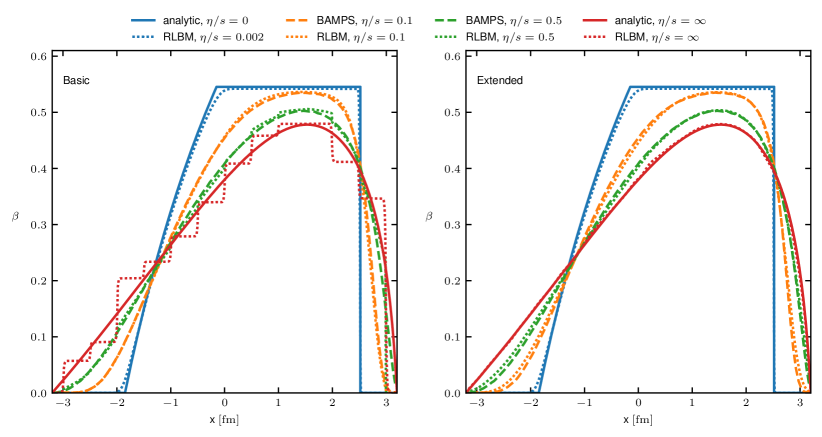
Figure 1: Riemann problem for an ultra-relativistic gas of particles for various viscous regimes. We show the macroscopic velocity profile $\beta=U^{x}/U^{0}$ at $t=3.2~{}\rm{fm}/c$, comparing the results of a RLBM model developed for the hydrodynamic regime Gabbana et al. (2020b) (left), and the high order scheme described in this work (right), which allows to significantly increase the accuracy of the numerical results in beyond-hydrodynamic regimes ($\eta/s>0.1$).

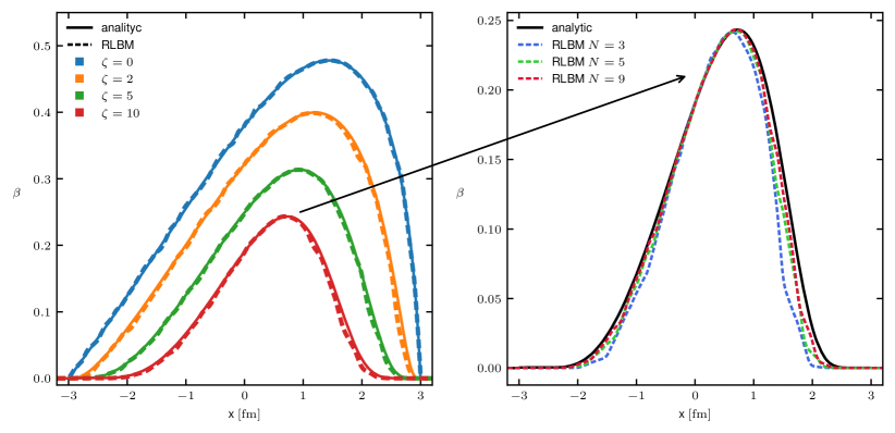
Figure 2: Riemann problem for a relativistic gas of particles in the free-streaming regimes at different values of the rest mass $m=(0,0.8,2,4)$ GeV, corresponding to $\zeta=(0,2,5,10)$. The left panel shows the macroscopic velocity profile $\beta=U^{x}/U^{0}$ at $t=3~{}\rm{fm}/c$, comparing the results of RLBM against analytic solutions. On the left panel, we use $N=3$, $K=19$ for $\zeta=(0,2)$, and $N=9$, $K=19$ for $\zeta=(5,10)$. The right panel shows the effect of increasing the radial quadrature for the case $\zeta=10$.

We start our numerical analysis by considering the relativistic Riemann problem. This problem describes a tube filled with a gas which initially is in two different states (particle number density $n$, temperature $T$ and macroscopic velocity $U^{\alpha}$) on the two sides of a membrane placed at $x=0$:

$$\left(n,T,U^{x}\right)=\begin{cases}n_{L},T_{L},0\quad x<0\\ n_{R},T_{R},0\quad x>0\\ \end{cases}\quad.$$ (1)

Once the membrane is removed, the system develops one-dimensional shock/rarefaction waves traveling along the $x-$axis. We use the same initial conditions as in Gabbana et al. (2020b), namely

$$\begin{cases}n_{\mathrm{L}}=13.575\,\mathrm{fm}^{-3},&T_{\mathrm{L}}=400\,\mathrm{MeV}\\ n_{\mathrm{R}}=1.65\,\mathrm{fm}^{-3},&T_{\mathrm{R}}=200\,\mathrm{MeV}\end{cases}\quad.$$ (2)

In these simulations we keep the ratio between the shear viscosity and the entropy density, $\eta/s$, fixed to a constant value. For the parameter $\eta$ we use the analytic expressions resulting from the first-order Chapman-Enskog expansion Gabbana et al. (2020a), while the entropy density is approximated using Cercignani and Kremer (2002)

$$s=n\left(\zeta\frac{K_{3}(\zeta)}{K_{2}(\zeta)}-\ln{\left(\frac{n}{n^{\rm eq}}\right)}\right)\quad,$$ (3)

with the equilibrium density given by

$$n^{\rm eq}=d_{\rm G}\frac{T^{3}}{2\pi^{2}}\zeta^{2}K_{2}(\zeta)\quad,$$ (4)

$d_{\rm G}=16$ being the degeneracy factor of gluons and $K_{\nu}(\zeta)$ the Modified Bessel function of second kind.

In the left panel of Fig. 1 we have reproduced, for reference, the results presented in Fig.1 from Gabbana et al. (2020b), showing the profile of the macroscopic velocity $\beta=U^{x}/U^{0}$ for a gas of massless particles in several different kinematic regimes. The two limiting cases, corresponding to the inviscid ($\eta/s\rightarrow 0$) and the ballistic ($\eta/s\rightarrow\infty$) regimes admit an analytic solution, whereas for intermediate regimes we compare the results against BAMPS (Boltzmann Approach to Multi-Parton Scatterings) Xu and Greiner (2007), which solves the Boltzmann equation using a Monte Carlo technique. The on-lattice RLBM model correctly reproduces the solution both in the inviscid and in the hydrodynamic regime ($\eta/s=0.1$). On the other hand, for larger values of $\eta/s$, as we move beyond the hydrodynamic regime, the macroscopic velocity profile develops artifacts which become most apparent in the ballistic limit. In the right panel of Fig. 1 we show that by employing high order off-lattice quadratures Ambruş and Blaga (2018) it is possible to improve the accuracy even in rarefied conditions. Here we have used a radial quadrature of order $N=3$ and an angular quadrature of order $K=15$ with $N_{K}=120$ discrete components (more details on the meaning of these values in Sec. V). We remark that the off-lattice model preserves the same level of accuracy of the on-lattice scheme also in the hydrodynamic regimes.

We now turn to the analysis of a relativistic gas of massive particles; we consider once again the initial conditions given in Eq. 2, with $m=(0,0.8,2,4)$ GeV. In the simulations we normalize quantities with respect to $T_{L}$ and $n_{L}$ (see Eq. (1)), corresponding to $\zeta=(0,2,5,10)$.

In the left panel of Fig. 2 we compare the results obtained in the free-streaming regime, corresponding to $\eta/s\rightarrow\infty$, against analytic solutions finding again a satisfactory match between the two.

One important remark is that, as the rest mass of the gas increases, we need to employ a higher order radial quadrature to match the same level of accuracy achieved, for example, in the massless case. This is shown in the right panel of Fig. 2, where we compare the results at $\zeta=10$ obtained by keeping fixed the angular quadrature at $K=19$ and varying the radial quadrature from $N=3$ (which is the value used for the massless case) up to $N=9$. The results show the improvements achieved by increasing the degree of accuracy of the radial quadrature.

We now further investigate how the accuracy of the method depends on the degree of angular and radial quadrature, studying the Riemann problem at different values of Knudsen number and relativistic coldness.

We use the same initial conditions given by Eq. (2). In order to assess the rarefied regime, we make use of the numerical Knudsen number, defined as follows:

$$\mathrm{Kn}=\frac{\tau\langle v\rangle}{L}\quad,$$ (5)

where $L$ defines the spatial resolution chosen for the grid, $\tau$ is the relaxation time, and $\langle v\rangle$ is a relative mean velocity, of order $1$ in lattice units. We consider a grid of $L=1600$ points representing a physical domain of $6.4~{}\rm{fm}$. As a reference, we take the results of RLBM simulations with a high resolution in terms of both grid and momentum discretization, namely $L=6400$, $N=9$ and $K=31$.

We define the L2-relative error with respect to the temperature field as

$$\epsilon=\frac{||T-T_{\rm hr}||_{2}}{||T_{\rm hr}||_{2}}\quad,$$ (6)

where “${\rm hr}$” refers to high resolution simulations.

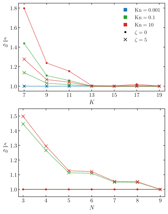
Figure 3: Discretization error versus the radial/angular quadrature at different Knudsen numbers and for different values of the relativistic coldness. The relative error $\epsilon$ (Eq. 6) is normalized with respect to its asymptotic value $\epsilon_{0}$, defined as $\epsilon_{0}=\epsilon(K=19)$ in the top panel and $\epsilon_{0}=\epsilon(N=9)$ in the bottom panel. Top: Effect of increasing the degree of the angular quadrature, while keeping the radial quadrature fixed at $N=3$. Bottom: Effect of increasing the degree of the radial quadrature, while keeping the angular quadrature fixed at $K=13$.

In the top panel of Fig. 3, we plot this observable versus the order of the angular quadrature $K$. All simulations run at fixed order of the radial quadrature, $N=3$, and different values of relativistic coldness, namely $\zeta=0$ and $\zeta=5$.

We can observe the effect of increasing the order of the angular quadrature $K$, by keeping fixed the radial quadrature to $N=3$. We notice that, as the Knudsen number is increased, a higher order leads to significant gains; interestingly this effect is more pronounced in the massless case. We also observe that in the hydrodynamic regime the accuracy is not affected by the quadrature degree.

In the bottom panel of Fig. 3 we consider instead the effect of varying the degree of the radial quadrature $N$, while keeping the angular quadrature fixed at $K=13$. We observe that in the massless case the error does not depend on the radial quadrature, regardless of the Knudsen number employed. On the other hand, for $\zeta=5$ it is necessary to increase the radial quadrature up to $N=9$ before saturating the error.

The intuition behind these results is as follows: since massless particles all travel at the speed of light, their discretized components necessarily lie on the surface of a sphere in momentum space. As a result, increasing the order of the angular quadrature offers a better approximation of momentum space. On the other hand, massive particles cover a finite range of velocities, thus requiring tuning of both the radial and the angular components (see Sec V.3 for more details).

II.3 Bjorken attractor

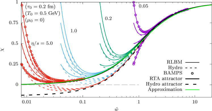
Figure 4: Dependence of $\chi$ (8) on $\tilde{w}$ (16) as obtained using RLBM (solid lines), hydro (dashed lines) and BAMPS (points). The initial conditions are $\tau_{0}=0.2\ {\rm fm}$ and $T_{0}=0.5\ {\rm GeV}$ in all cases, while $\eta/s$ takes the values $5$ (red), $1$ (blue), $0.2$ (green) and $0.05$ (purple). The hydro results are obtained by directly integrating Eq. (9). The BAMPS data are taken from Ref. Ambrus et al. (2021). The RLBM algorithm employs $2$ points along the radial direction, $20$ points for $v_{z}=\cos\theta$ and $1$ point in the azimuthal direction, as discussed in Refs. Ambruş and Blaga (2018); Ambruş and Guga-Roşian (2019). The hydro attractor is shown with the dashed black line. The RTA attractor obtained using our code (solid black line) is in excellent agreement with the analytical approximation from Ref. Romatschke, Paul (2018a) (solid green line).

The method described so far is based on a uniform Cartesian grid. However, a similar procedure applies to curvilinear coordinates as well Ambruş and Blaga (2018); Ambruş and Guga-Roşian (2019), which represent the most natural choice for a variety of relativistic flow problems. In this subsection we focus on such one case, namely the Bjorken model Bjorken (1983), which is particularly relevant to QGP experiments. Indeed, the existence of Bjorken attractors Heller and Spalinski (2015) and the details of their structure have received significant attention in the recent years, for they provide valuable information on the initial conditions right after the collisions, the onset of fluid-dynamic behavior and also on the material properties of the QGP state of matter (see Ref. Soloviev, Alexander (2022) for a recent review). The evolution of the system at very early times (the pre-equilibrium phase) along the attractor allows one to estimate the work done by the QGP plasma against longitudinal expansion, which leads to the overall cooling of the fireball Kurkela et al. (2019). Moreover, the entropy production in this pre-equilibrium phase can be used to increase the accuracy of the connection between the initial state energy and of the overall particle yields Giacalone et al. (2019). Another effect of the pre-equilibrium stage is related to the inhomogeneous cooling of the initial state, leading to modifications of the transverse profile that decrease its eccentricity, thus affecting the buildup of flow harmonics, such as elliptic flow $v_{2}$, during the transverse expansion phase Ambrus et al. (2022).

The focus of this section is on the early-time dynamics of the fireball induced by the rapid longitudinal expansion, which is well described by Bjorken’s approximation of longitudinal boost invariance. For simplicity, we focus on the flow of massless particles (with equation of state $\epsilon=3P$) with constant $\eta/s$.

Neglecting the dynamics in the transverse plane, the velocity profile satisfying boost-invariance along the $z$ direction is

$$U^{\alpha}\partial_{\alpha}=\frac{1}{\tau}(t\partial_{t}+z\partial_{z})=\partial_{\tau},$$ (7)

where $\tau=\sqrt{t^{2}-z^{2}}$ is the Bjorken time. Employing the Bjorken coordinates $(\tau,x,y,\eta_{s})$, where $\eta_{s}={\rm atanh}(z/t)$ is the pseudorapidity, the particle four flow $N^{\mu}$ and stress-energy tensors $T^{\mu\nu}$ reduce to $N^{\tau}=n$, $N^{x}=N^{y}=N^{\eta}=0$, while $T^{\mu\nu}={\rm diag}(\epsilon,P_{T},P_{T},\tau^{-2}P_{L})$. The diffusion current vanishes, while the pressure deviator $\pi^{\mu\nu}$ takes a diagonal form, $\pi^{\mu\nu}={\rm diag}(0,-\pi_{d}/2,-\pi_{d}/2,\tau^{-2}\pi_{d})$, where $\pi_{d}=\frac{2}{3}(P_{L}-P_{T})$. Our focus in this section will be on the function

$$\chi=\frac{P_{L}}{P_{T}}=\frac{P+\pi_{d}}{P-\frac{1}{2}\pi_{d}},$$ (8)

representing the ratio between the longitudinal and transverse pressures.

The macroscopic equations $\nabla_{\mu}N^{\mu}=0$ and $\nabla_{\mu}T^{\mu\nu}=0$ reduce to

$$\tau\frac{\partial(\tau n)}{\partial\tau}= 0,$$ (9a)

$$\tau\frac{\partial\epsilon}{\partial\tau}+\epsilon+P+\pi_{d}= 0.$$ (9b)

The equation for $$\pi_{d}$$ can be derived in the frame of the Israel-Stewart second order hydrodynamics Israel (1976); Israel and Stewart (1976), or directly from the Boltzmann equation (20) using the Chapman-Enskog method Jaiswal (2013),

$$\tau\frac{\partial\pi_{d}}{\partial\tau}+\left(\lambda+\frac{\tau}{\tau_{R}}\right)\pi+\frac{16}{15}P=0,$$ (9c)

where $\lambda=38/21$ and $\tau_{R}=5\eta/4P$ is the Anderson-Witting relaxation time. Since $P$ and $\pi_{d}$ depend only on $\tau$, Eq. (9) can be solved straightforwardly, e.g. using Runge-Kutta time stepping.

The evolution of $\pi_{d}$ can be obtained from the kinetic equation by writing Eq. (20) with respect to the Bjorken coordinates, taking into account the degrees of freedom $p=p^{\tau}$, $v_{z}=\tau p^{\eta}/p$ and $\varphi=\arctan(p^{y}/p^{x})$ Kurkela et al. (2019)

$$\left(\partial_{\tau}-\frac{v_{z}(1-v_{z}^{2})}{\tau}\partial_{v_{z}}-\frac{v_{z}^{2}p}{\tau}\partial_{p}\right)f=-\frac{v^{\mu}u_{\mu}}{\tau_{R}}(f-f^{\rm eq}),$$ (10)

where $v_{z}=\cos\theta$ in the language of Sec. V.3. For simplicity, $f^{\rm eq}$ is taken as the Maxwell-Jüttner distribution given in Eq. (40), which reduces in the case of massless particles to

$$f^{\rm eq}=\frac{n}{8\pi T^{3}}\exp\left(-\frac{p^{\alpha}U_{\alpha}}{T}\right).$$ (11)

At initial time, the distribution function is set to the Romatschke-Strickland distribution Romatschke and Strickland (2003); Florkowski et al. (2013),

$$f_{\rm RS}=\frac{ge^{\alpha_{0}}}{(2\pi)^{3}}\exp\left[-\frac{1}{\Lambda_{0}}\sqrt{(p\cdot u)^{2}+\xi_{0}(p\cdot\hat{z})^{2}}\right],$$ (12)

where $\hat{z}^{\mu}$ is the unit-vector along the rapidity coordinate and $g=16$ is the number of gluonic degrees of freedom. The parameters $\alpha_{0}$, $\Lambda_{0}$ and $\xi_{0}$ can be used to set the initial values $n_{0}$, $P_{0}$ and $\chi_{0}$, as indicated in Eqs. (11)–(13) of Ref. Ambrus et al. (2021).

In solving Eq. (10), it is convenient to take advantage of the azimuthal symmetry of the setup in both the coordinate and the momentum space. This allows only one point to be taken along the azimuthal direction $\varphi$, while $v_{z}$ can be discretized using the Gauss-Legendre quadrature of order $Q_{\xi}$ Romatschke et al. (2011); Ambruş and Blaga (2018). Using the Gauss-Laguerre quadrature rules, $p$ is discretized using only $N_{L}=2$ points, namely $p_{1}=2T_{0}$ and $p_{2}=6T_{0}$, where $T_{0}$ is taken as the initial temperature Ambruş and Blaga (2018). Therefore, the total number of discrete momentum vectors employed for the simulations presented in this subsection is $2Q_{\xi}$. The expansions of $f^{\rm eq}$ and $f_{\rm RS}$ analogous to the one in Eq. (28) can be found in Refs. Ambruş and Blaga (2018) and Ambruş and Guga-Roşian (2019), respectively.

Labeling the discrete populations $f_{jk}$ with $1\leq j\leq Q_{\xi}$ and $1\leq k\leq N_{L}$, the derivatives of $f$ with respect to $v_{z}$ and $p$ can be computed via projection onto the Legendre and Laguerre polynomials, respectively leading to linear relations. In the former case, we have

$$\left[\frac{\partial[v_{z}(1-v_{z}^{2})f]}{\partial v_{z}}\right]_{jk}=\sum_{j^{\prime}=1}^{Q_{\xi}}\mathcal{K}^{P}_{j,j^{\prime}}f_{j^{\prime},k},$$ (13)

where the kernel matrix $\mathcal{K}^{P}_{j,j^{\prime}}$ depending only on $Q_{\xi}$ can be precomputed. The explicit expression of its elements can be found in Eq. (3.54) of Ref. Ambruş and Blaga (2018). For the derivative with respect to $p$, we can take advantage that $Q_{L}=2$ is fixed and write

$$\left[\frac{1}{p^{2}}\frac{\partial(fp^{3})}{\partial p}\right]_{j,\frac{3}{2}\mp\frac{1}{2}}=\pm\frac{1}{2}f_{j1}\pm\frac{3}{2}f_{j2},$$ (14)

where the upper and lower signs correspond to $k=1$ and $2$, respectively.

We now compare the hydro and RTA solutions, focusing on the function $\chi$ given in Eq. (8). For further validation, we consider a comparison with the Boltzmann Approach to Multi-Parton Scattering (BAMPS), which is a particle-based stochastic method Xu and Greiner (2005); Xu et al. (2008). The initial state is prepared at vanishing chemical potential, such that $n_{0}\equiv n(\tau_{0})=gT_{0}^{3}/\pi^{2}$. Subsequently, the conservation of the particle number density implied by Eq. (9a) enforces $n(\tau)=n_{0}\tau_{0}/\tau$, leading to a non-trivial evolution of the chemical potential $\mu=T\ln(n\pi^{2}/gT^{3})$. Enforcing a constant ratio between the shear viscosity $\eta=\frac{4}{5}\tau_{R}P$ and the entropy density $s=(\epsilon+P-\mu n)/T$ fixes the relaxation time to

$$\tau_{R}=\frac{5\eta/s}{T}\left(1+\frac{3}{4}\ln\frac{\tau^{4/3}P}{\tau_{0}^{4/3}P_{0}}\right).$$ (15)

In order to describe the evolution of $\chi$, it is convenient to employ the scaling variable $\tilde{w}$ defined via Blaizot and Yan (2021a)

$$\tilde{w}=\frac{5\tau}{4\pi\tau_{R}}.$$ (16)

In the case of a parton gas, for which $\mu=0$ at all times, the above reduces to $\tilde{w}=\tau T/(4\pi\eta/s)$ Kamata et al. (2020). Within the parton gas model, it was pointed out in Refs. Heller and Spalinski (2015); Blaizot and Yan (2021b, a) for the case of the hydro equations and in Refs. Heller et al. (2018); Blaizot and Yan (2018); Strickland (2018); Behtash et al. (2019); Blaizot and Yan (2021a) for kinetic theory that $\chi$ generally exhibits a decay from an arbitrary initial condition $\chi_{0}$ onto an attractor solution that bridges the free-streaming ($\tilde{w}=0$) and the hydrodynamic ($\tilde{w}\rightarrow\infty$) fixed points. Figure 4 shows that a similar phenomenon occurs in the case of the ideal gas considered here. Here we present the numerical results for the evolution of $\chi$ corresponding to two sets of $4\times 4$ simulations, one set for the RLBM results (solid lines) and another one for hydro (dashed lines). In addition, BAMPS results taken from Ref. Ambrus et al. (2021) are shown with empty circles for a subset of curves. The initial time and temperature are set to $\tau_{0}=0.2\ {\rm fm}$ and $T_{0}=0.5\ {\rm GeV}$, respectively, while $\eta/s$ takes the values $5$ (red) $1$ (blue) $0.2$ (green) and $0.05$ (purple), resulting in four different values of $\tilde{w}_{0}$. For each value of $\eta/s$, four initial values of $\chi_{0}$ are considered, namely $1$, $0.75$, $0.5$ and $0.25$.

The RTA and hydro attractor curves are shown with black solid and dashed lines, respectively. The analytical approximation for the RTA attractor derived in Ref. Romatschke, Paul (2018a) is also represented using a solid green line and is almost everywhere overlapped with our numerical solution. The approach to the attractor can be clearly seen for both RLBM and hydro and most notably, these attractors differ when $\tilde{w}\lesssim 1$. In particular, it can be seen that the attractor solution for hydro gives $\chi<0$ corresponding to an unphysical negative longitudinal pressure at small $\tilde{w}$. The agreement between hydro and RTA is restored when $\tilde{w}\gtrsim 1$, both at the level of the attractor solutions and of the dynamics of the approach to the attractor. The BAMPS results are in excellent agreement with the RLBM solution throughout the entire flow regime.

II.4 Anisotropic vortical flow

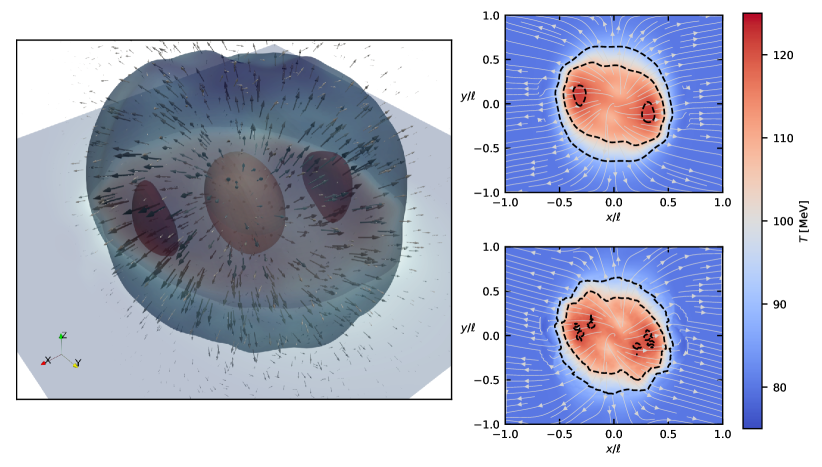
Figure 5: Simulation of a vortical flow, using the initial conditions described in Eq. 17 and Eq. II.4, for a box of side $\ell=20~{}\rm{fm}$ . The three-dimensional figure in the left panel reports the temperature field after $t=4~{}\rm{fm/c}$. We also provide a two-dimensional view on the $z=0$ plane at the same time step, comparing the results provided by the model presented in this work (top-right), with the results obtained with a previous version of the model restricted to the simulation of hydrodynamic regimes (bottom-right). The bottom-right panel shows that the interaction between QGP and the rarefied background gives origin to artifacts (”scars” in the $(x/\ell,y/\ell)\sim(\pm 0.5,0.0)$ region and a general irregularity in the contour lines), not observed in the present model.

Recent measurements made by the STAR collaboration at the level of the decay products of the $\Lambda$ hyperons revealed that the quark-gluon plasma (QGP) formed during heavy ion collisions acquires a global polarization Adamczyk et al. (2017); Adam et al. (2018). Possible mechanisms leading to the polarization of the QGP constituents are the quantum chiral magnetic and chiral vortical effects Fukushima et al. (2008); Kharzeev et al. (2016) (see also Ref. Ambrus and Chernodub (2022) for an interplay between chiral and helical Ambrus and Chernodub (2019) vortical effects). Taken together, these effects can explain the global polarization of the $\Lambda$ hyperons by means of a non-vanishing magnetic field or vorticity on the freezeout hypersurface. While the relevance of the chiral magnetic effect strongly depends on the lifetime of the magnetic field in the QGP fireball, vorticity is expected to be long-lived, decaying only due to dissipation caused by shear. Studies have estimated the vorticity to have a sizeable magnitude at freezeout Becattini et al. (2015). The polarization induced by vorticity can be estimated using the Wigner function formalism Becattini et al. (2013). Modeling the dynamics of vorticity using hydrodynamics gives an excellent match with the experimental data for the global polarization Karpenko and Becattini (2017) (i.e., along the total angular momentum vector $\bm{J}_{\rm sys}$). The detailed structure of the local (differential) polarization along both the beam (or longitudinal) and the $\bm{J}_{\rm sys}$ directions proves to be more challenging to reproduce, since non-equilibrium effects such as the coupling of spin with the thermal shear can make significant contributions to polarization Becattini et al. (2021a); Liu and Yin (2021); Fu et al. (2021); Becattini et al. (2021b).

In this section, we show an example application of our new scheme aimed at simulating the dynamics of an initial vortex configuration in the more simplistic setup ignoring the longitudinal expansion (this was addressed in the frame of the Bjorken model in Sec. II.3).

We consider an ultra-relativistic gas in a cubic grid of side $20~{}\rm{fm}$, with open boundary conditions. Following previous works Friman et al. (2019); Gabbana et al. (2020c), we initialize the density and temperature fields with an asymmetric Gaussian shape:

$$T =T_{b}+T_{0}\,g(x,y,z)\;,$$ (17)

$$n =n_{b}+n_{0}\,g(x,y,z)\;,$$

$$g(x,y,z) =\exp\left(-\frac{x^{2}}{2\sigma_{x}^{2}}-\frac{y^{2}}{2\sigma_{y}^{2}}-\frac{z^{2}}{2\sigma_{z}^{2}}\right)\;.$$

Here $T_{b}=80~{}\rm{MeV}$, $n_{b}=10^{-3}~{}\rm{fm}^{-3}$ are background values for temperature and density, while $T_{0}=200~{}\rm{MeV}$, $n_{0}=4\times 10^{-3}~{}\rm{fm}^{-3}$. We choose $\sigma_{x}=1~{}\rm{fm}$, $\sigma_{y}=2.6~{}\rm{fm}$ and $\sigma_{z}=2~{}\rm{fm}$. The initial velocity field is chosen as follows:

$$U_{x}/U_{0} =-\frac{y}{\sqrt{x^{2}+y^{2}}}\tanh{\left(\frac{\sqrt{x^{2}+y^{2}}}{r_{0}}\right)}\;,$$

$$U_{y}/U_{0} =\phantom{+}\frac{x}{\sqrt{x^{2}+y^{2}}}\tanh{\left(\frac{\sqrt{x^{2}+y^{2}}}{r_{0}}\right)}\;,$$ (18)

$$U_{z}/U_{0} =0\,$$

with $r_{0}=6~{}\rm{fm}$. We apply a cut-off radius $R=3~{}\rm{fm}$ in the $z=0$ plane, outside of which the velocity field is set to zero.

The central ellipsoid represents the QGP formed in the collision between heavy nuclei. The highly compressed bulk of the system rotates and expands, cooling down in the process. In a later stage, the ”fireball” further expands and cools down, so that the system exits the hydrodynamic regime and enters a weakly interacting rarefied regime known as ”freeze-out”.

The ”freeze-out” regime is classified in terms of $\eta/s$, which in QGP is found to reach the theoretical lower bound of $1/4\pi$ Kovtun et al. (2005).

In order to characterize this effect, we have parametrized $\eta/s$ as a function of the local temperature, using the following expression Zhang et al. (2019); Niemi et al. (2011):

$$\eta/s=\begin{cases}0.681-0.0594\left(\frac{T}{T_{R}}\right)-0.544\left(\frac{T}{T_{R}}\right)^{2}\;&T<T_{R}\\ \frac{1}{4\pi}\;&T\geq T_{R}\end{cases}$$ (19)

with $T_{R}=175~{}\rm{MeV}$. In Fig. 5, we show the results of the simulation at $t=4~{}\rm{fm/c}$, with the results obtained using a high order off-lattice scheme ($N=3$, $K=15$) on the top right panel, and the results of the on-grid scheme in the bottom left panel.

The comparison shows that the high order method allows to cure the artifacts clearly visible in the lower panel, in particular at the boundaries of the fireball where the fluid starts to interact with the rarefied region.

III Performance data

In this section we give a short overview of the performances of the numerical model. The present algorithm has been implemented for the benchmark described in Sec. II.4 on a single V100-GPU machine using double-precision arithmetics and standard practice optimizations Calore et al. (2016a, b), delivering about 60 MLUPS (Million Lattice UPdates per Second) on a $128^{3}$ cubic grid with $N_{\rm pop}=128$ discrete velocities. This means that the state of the system is advanced over $30$ time steps in a second wall-clock GPU time. For a computational box $10~{}\rm{fm}$ in side, this corresponds to a lattice spacing of about $0.1~{}\rm{fm}$ and a time-step of about $0.1~{}\rm{fm/c}$. The performance of our code is comparable to that of the GPU implementation of the ideal hydro code reported in Ref. Gerhard, Jochen and Lindenstruth, Volker and Bleicher, Marcus (2013), while giving access to off-equilibrium dynamics, such as dissipation.

Notably, as shown in Fig. 6, the performance scales linearly with the inverse number of components used in the discretization of the momentum space $1/N_{\rm pop}$, reaching down to about 20 MLUPS for the case $N_{\rm pop}=480$. This is an important result, as it shows that the code suffers no performance extra-penalty in going from the hydro to the quasi-ballistic regime.

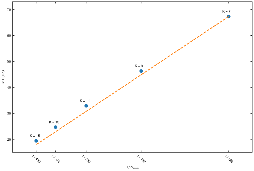
Figure 6: Performance scaling with respect to the number of discrete velocities. Figures refer to quadratures for a ultra-relativistic gas with a radial quadrature of degree $N=3$ and an angular quadrature of degree $K$ (see labels in the figure). The measured performances (blue dots) are measured in Million Lattice UPdates per Second. The dashed line represents the linear scaling with respect to $N_{\rm pop}=128$.

As a result, a simulation spanning one million time-steps, i.e. $10^{5}~{}\rm{fm/c}$, would complete in roughly $3\times 10^{4}$ seconds, namely about half day. Since, as already observed, our method seamlessly describes both hydrodynamic and quasi-ballistic regimes, it can efficiently simulate the long-term evolution of laboratory QGP well into the freeze-out regime and possibly beyond.

Indeed, with suitable coupling to Monte Carlo schemes, by sampling particle position and momenta from the RLBM solution, Di Staso et al. (2016), it may also be possible to describe the re-hadronization stage, in which quarks bind back into hadrons Fries et al. (2003); Molnár and Voloshin (2003); Greco et al. (2003); Petersen, Hannah and Steinheimer, Jan and Burau, Gerhard and Bleicher, Marcus and Stöcker, Horst (2008); Weil, J. and others (2016). Compared to Monte-Carlo-based implementations such as BAMPS Xu and Greiner (2007); Bouras et al. (2009); Gallmeister, K. and Niemi, H. and Greiner, C. and Rischke, D. H. (2018); Ambrus et al. (2021), which suffer from statistical noise, our scheme can be expected to be between $1$ and $2$ orders of magnitude faster.

On a mid-term perspective, one may realistically project the current data to large-scale massive parallel GPU architectures, such as the Nvidia A100 series. For instance, recent work on multiphase non-relativistic fluids shows that classical Lattice Boltzmann schemes with 27 discrete populations can attain up to 100 GLUPS on grids with several billion grid points, using large clusters with hundreds Nvidia A100 GPUs Bonaccorso et al. (2022); Succi et al. (2019).

Based on the linear dependence of the GPU performance on the inverse number of populations, one can estimate about $20\div 5$ GLUPS for the case of $100\div 400$ discrete velocities. The same ballpark estimate is obtained by upscaling the current 60 MLUPS to 6 GLUPS on a hundred-GPUs cluster. This means several updates per second of grids with billion grid points, hence enabling the direct simulation of QGP over three decades in space and twice as many in time, within a few days wall-clock time.

IV Discussion

Relativistic kinetic theory is ubiquitous to several fields of modern physics, finding application both at large scales, in the realm of astrophysics, down to atomic scales (e.g., in the study of the electron properties of graphene) and further down to subnuclear scales, in the realm of quark-gluon plasmas. This motivates the quest for powerful and efficient computational methods, able to accurately study fluid dynamics in the relativistic regime as well as the transition to beyond hydrodynamics, in principle all the way down to ballistic regimes.

In this work we have introduced a lattice kinetic scheme which extends the range of applicability of RLBM to a wider range of kinetic parameters, allowing for the simulation of relativistic gases of massive particles in rarefied conditions.

The present scheme builds on high order quadrature rules developed to separately discretize the radial and the angular coordinates in the momentum space. These quadratures are in general not compatible with a Cartesian grid, therefore introducing the need for an interpolation scheme in the streaming step. We show that by increasing the degree of the radial and angular quadrature it is possible to tune the accuracy of the numerical scheme to the given kinetic parameters.

By analyzing shock waves in a quark-gluon plasma we have shown that in order to achieve good accuracy in rarefied conditions, the order of the radial quadrature must increase at increasing values of the relativistic coldness. This means that the non-relativistic regime is more demanding than the relativistic one, which is in line with the fact that non-relativistic particles move in a broader range of speeds as compared to the relativistic ones.

From a computational point of view, RLBM retains the advantages of standard Lattice Boltzmann schemes, making it an ideal candidate for efficient implementations on massively parallel architectures.

We have evaluated the performances of a GPU implementation of the method, showing that the computational cost grows linearly with the number of discrete components employed in the momentum space discretization.

This paves the way to the systematic study of heavy-ion collisions observables such as the $p_{T}$ dependence of the flow harmonics $v_{n}(p_{T})$ Romatschke, Paul (2018b) or hadron polarization Karpenko and Becattini (2017) within kinetic theory. Extensions of the current scheme to the case of non-ideal fluids can be performed along the lines discussed in Ref. Romatschke (2012), allowing phenomena related to the QCD phase transition to be explored through large-scale simulations Adamczyk, L. and others (2014); Habich, Mathis and Romatschke, Paul (2014); Nahrgang, Marlene and Bluhm, Marcus and Schaefer, Thomas and Bass, Steffen A. (2019).

While a fair comparison between RLBM and Monte Carlo approaches is somehow ill-posed, since the latter can handle non-equilibrium effects in full, for systems where the relaxation-time approximation applies, RLBM can be expected to offer one or two orders of magnitude speedup over Monte Carlo methods.

To conclude, the present results lay the ground to the computationally efficient large-scale simulations of beyond-hydrodynamic regimes in the framework of QGP experiments. They may also find profitable use in the study of quasi-ballistic electron flows in graphene and possibly also for relativistic flows of astrophysical interest. In addition, the implementation of the Boltzmann-Vlasov equation for resistive relativistic magnetohydrodynamics Denicol, Gabriel S. and Molnár, Etele and Niemi, Harri and Rischke, Dirk H. (2019); Bacchini, Fabio and Arzamasskiy, Lev and Zhdankin, Vladimir and Werner, Gregory R. and Begelman, Mitchell C. and Uzdensky, Dmitri A. (2022) is straightforward via the addition of the electromagnetic forcing term, and this in turn might unlock applications in the realm of Plasma Wakefield Acceleration Parise,G. and Cianchi,A. and Del Dotto,A. and Guglietta,F. and Rossi,A. R. and Sbragaglia,M. (2022).

V Methods

In this section we provide full details on the definition of the Relativistic Lattice Boltzmann Method, with particular emphasis posed on the momentum space discretisation, which is crucial in order to support the simulation of dynamics at large values of the Knudsen number. We start by introducing the notation and with a brief introduction to the main elements of relativistic kinetic theory.

V.1 Relativistic Kinetic Theory

We consider a gas of particles with mass $m$ in a $(3+1)$ Minkowski space-time, with metric $\eta^{\alpha\beta}={\rm diag}(+,-,-,-)$. We adopt Einstein’s summation convention, with Greek indices running from $0$ to $3$, and latin ones from $1$ to $3$, respectively. We also use natural units: $c=k_{\rm B}=\hbar=1$.

Our starting point in the development of the model is the relativistic Boltzmann equation, in the single-relaxation time approximation of Anderson and Witting Anderson and Witting (1974a, b)

$$p^{\alpha}\partial_{\alpha}f=-\frac{U^{\alpha}p_{\alpha}}{\tau}\left(f-f^{\rm eq}\right)\quad.$$ (20)

This equation describes the evolution of the particle distribution function $f(x^{\alpha}=(t,\mathbf{x}),p^{\alpha}=(p^{0},\mathbf{p}))$, accounting for the number of particles per unit volume in the 6-dimensional single-particle phase space $\mathop{}\!\mathrm{d}^{3}x\mathop{}\!\mathrm{d}^{3}p$.

$U^{\alpha}$ is the macroscopic fluid velocity, $\tau$ is the (proper)-relaxation time and $f^{\rm eq}$ is the equilibrium distribution function:

$$f^{\rm eq}(p^{\alpha},U^{\alpha},T)=\frac{(2\pi)^{-3}g}{\exp{\left(\frac{p^{\alpha}U_{\alpha}-\mu}{T}\right)}+\varepsilon}\quad,$$ (21)

where $\mu$ is the chemical potential, $g$ is the number of degrees of freedom per constituent, and $\varepsilon$ is a parameter selecting between the Maxwell-Jüttner ($\varepsilon=0$), Fermi-Dirac ($\varepsilon=1$) and Bose-Einstein ($\varepsilon=-1$) distributions. From now on, we will be considering the Maxwell-Jüttner statistics ($\varepsilon=0$).

The chemical potential $\mu$ can be expressed in terms of the particle number density. For the Maxwell-Jüttner statistics, we have

$$\frac{g}{(2\pi)^{3}}e^{\mu/T}=\frac{n}{4\pi T^{3}\zeta^{2}K_{2}(\zeta)}\quad,$$ (22)

with $n$ the particle number density, and $K_{\nu}$ the modified Bessel function of second kind of index $\nu$.

The hydrodynamic fields are related to the lower order moments of the distribution function, in particular the first and second order moments, namely the particle flow $N^{\alpha}$ and energy momentum tensor $T^{\alpha\beta}$,

$$N^{\alpha}=\int p^{\alpha}f\frac{\mathop{}\!\mathrm{d}^{3}p}{p^{0}}\quad,$$ (23)

$$T^{\alpha\beta}=\int p^{\alpha}p^{\beta}f\frac{\mathop{}\!\mathrm{d}^{3}p}{p^{0}}\quad.$$ (24)

The moments of the distribution can be put in relation to the macroscopic fields via the Landau-Lifschitz Landau and Lifshitz (1987) decomposition:

$$N^{\alpha} =nU^{\alpha}-\frac{n}{P+\epsilon}q^{\alpha}\quad,$$ (25)

$$T^{\alpha\beta} =(P+\epsilon+\varpi)U^{\alpha}U^{\beta}-(P+\varpi)\eta^{\alpha\beta}+\pi^{<\alpha\beta>}\quad;$$ (26)

where $P(\varpi)$ is the hydrostatic (dynamic) pressure, $q^{\alpha}$ the heat flux, $\epsilon$ the energy density and $\pi^{<\alpha\beta>}$ the pressure deviator. By computing the integrals in Eq. 23 and 24 at equilibrium, and matching them with the known expressions of the equilibrium moments $N^{\alpha}_{\mathrm{eq}}$ and $T^{\alpha\beta}_{\mathrm{eq}}$, one finds the following ideal Equation of State (EoS):

$$\epsilon=P\left(\zeta\frac{K_{3}(\zeta)}{K_{2}(\zeta)}-1\right)\quad,\quad P=nT\quad,$$ (27)

This reduces to the familiar expressions $\epsilon=3P$ in the ultrarelativisitc case ($\zeta\to 0$) and $P=(3/2)nT$ in the non-relativistic one ($\zeta\to\infty$), respectively.

V.2 Relativistic Lattice Boltzmann Method

We start, after an adimensionalization of variables, by considering a $N$-truncated expansion of the Maxwell-Jüttner distribution (Eq. 40) onto a tensorial basis of rank-$k$, $\mathbf{J}^{(k)}(p^{\mu})$:

$$f^{\rm eq}(p^{\mu},U^{\mu},T)=\omega(p^{0})\sum_{k=0}^{N}\mathbf{a}^{(k)}(U^{\mu},T)\cdot\mathbf{J}^{(k)}(p^{\mu})\quad,$$ (28)

where “$\cdot$” represents full tensor contraction. These tensors $\mathbf{J}^{(k)}$ are built as orthogonal polynomials in the variable $p^{\mu}$ with respect to a weighting function $\omega(p^{0})$, by using a standard Gram-Schmidt procedure, and can be shown to satisfy the following orthonormality condition:

$$\int\omega(p^{0})\,\mathbf{J}^{(l)}_{\alpha}(p^{\mu})\,\mathbf{J}^{(k)}_{\beta}(p^{\mu})\frac{\mathrm{d}^{3}p}{p^{0}}=\delta^{lk}\delta_{\alpha\beta}\quad,$$ (29)

where $\alpha=\{\alpha_{1},\dots,\alpha_{l}\}$ and $\beta=\{\beta_{1},\dots,\beta_{k}\}$ are collective tensorial indices introduced for notational conciseness. A detailed discussion and derivation of this set of orthogonal polynomials can be found in Gabbana et al. (2020a). The expansion coefficients in Eq. 28 are defined as

$$\mathbf{a}^{(k)}(U^{\mu},T)=\int f^{\rm eq}(p^{\mu},U^{\mu},T)\,\mathbf{J}^{(k)}(p^{\mu})\frac{\mathop{}\!\mathrm{d}^{3}p}{p^{0}}\quad.$$ (30)

The choice of the weight function $\omega(p^{0})$ is instrumental: by taking it as the equilibrium distribution in the rest frame, it is possible to establish a direct link between each coefficient $\mathbf{a}^{(k)}$ and the corresponding $k-th$ moment of the distribution function.

Next, we define a quadrature rule satisfying the requirement of preserving all the moments of the distribution up to order $N$. The quadrature is obtained as product of Gaussian quadratures: we consider a radial quadrature of degree $N$, consisting of $(N+1)$ discrete components, and an angular quadrature of degree $K$, consisting of $N_{K}$ discrete components (see Sec. V.3 for full details). This results in a set of $N_{pop}=N_{K}(N+1)$ discrete momenta $\{p^{\mu}_{i}\}$ and corresponding weights $\{w_{i}\}$, which allows to define the discretized version of the equilibrium distribution

$$f^{\rm eq}_{i}=f^{\rm eq}(p^{\mu}_{i},U^{\mu},T)=w_{i}\sum_{k=0}^{N}\mathbf{a}^{(k)}(U^{\mu},T)\cdot\mathbf{J}^{(k)}(p^{\mu}_{i})\quad.$$ (31)

By construction this recovers all the moments of the distribution function in the continuum up to order $N$, and it follows that integrals in Eq. 23 and  24 can be computed exactly (i.e. equality holds) via discrete sums:

$$N^{\alpha}=\sum_{i}^{N_{\rm pop}}p^{\alpha}_{i}f_{i}\quad,\quad T^{\alpha\beta}=\sum_{i}^{N_{\rm pop}}p^{\alpha}_{i}p^{\beta}_{i}f_{i}\quad,$$ (32)

where $f_{i}=f_{i}(\bm{x},t)=f(p^{\mu}_{i},\bm{x},t)$. By combining the quadrature-based discretization of the momentum space with a forward-Euler discretization in time with time-step $\Delta t$, it is possible to derive the discrete relativistic Lattice Boltzmann equation:

$$f_{i}(\bm{x}+\bm{v}_{i}\Delta t,t+\Delta t)=f_{i}(\bm{x},t)+\Delta t~{}\frac{p_{i}^{\alpha}U_{\alpha}}{p^{0}_{i}\tau}(f_{i}^{\rm eq}-f_{i}(\bm{x},t))\;,$$ (33)

where $\bm{v}_{i}=\bm{p}_{i}/p^{0}_{i}$.

We conclude this section with a quick summary of the algorithmic procedure needed to advance Eq. 33 over a single time step, based on the stream&collide paradigm.

Starting from a suitable initialization $f_{i}(t=0)$, at each time step the discrete populations freely stream to the corresponding lattices sites:

$$f_{i}^{*}(\bm{x},t)=f_{i}(\bm{x}-\bm{v}_{i}\Delta t,t)\quad,$$ (34)

This moves information from each lattice point at a distance $\Delta_{i}\bm{x}=\bm{v}_{i}\Delta t$. Clearly, an interpolation is required whenever $\bm{x}-\Delta_{i}\bm{x}$ does not fall on a grid point, in order to infer the values of the populations at the nodes of the actual Cartesian grid, based on their off-lattice values. In this work we adopt a simple trilinear interpolation scheme:

$$\begin{split}f_{i}(\bm{x}-\bm{v}^{i}\Delta t,t)=&\frac{1}{\Delta x\,\Delta y\,\Delta z}\times\Big{\{}\\ &f_{i}(\bm{x}-\bm{r}_{x}-\bm{r}_{y}-\bm{r}_{z},t)\big{(}\phantom{\Delta x-{}}\Delta t\big{|}v^{i}_{x}\big{|}\big{)}\big{(}\phantom{\Delta y-{}}\Delta t\big{|}v^{i}_{y}\big{|}\big{)}\big{(}\phantom{\Delta z-{}}\Delta t\big{|}v^{i}_{z}\big{|}\big{)}\,+\\ &f_{i}(\bm{x}\phantom{{}-\bm{r}_{x}}-\bm{r}_{y}-\bm{r}_{z},t)\big{(}\Delta x-\Delta t\big{|}v^{i}_{x}\big{|}\big{)}\big{(}\phantom{\Delta y-{}}\Delta t\big{|}v^{i}_{y}\big{|}\big{)}\big{(}\phantom{\Delta z-{}}\Delta t\big{|}v^{i}_{z}\big{|}\big{)}\,+\\ &f_{i}(\bm{x}-\bm{r}_{x}\phantom{{}-\bm{r}_{y}}-\bm{r}_{z},t)\big{(}\phantom{\Delta x-{}}\Delta t\big{|}v^{i}_{x}\big{|}\big{)}\big{(}\Delta y-\Delta t\big{|}v^{i}_{y}\big{|}\big{)}\big{(}\phantom{\Delta z-{}}\Delta t\big{|}v^{i}_{z}\big{|}\big{)}\,+\\ &f_{i}(\bm{x}-\bm{r}_{x}-\bm{r}_{y}\phantom{{}-\bm{r}_{z}},t)\big{(}\phantom{\Delta x-{}}\Delta t\big{|}v^{i}_{x}\big{|}\big{)}\big{(}\phantom{\Delta y-{}}\Delta t\big{|}v^{i}_{y}\big{|}\big{)}\big{(}\Delta z-\Delta t\big{|}v^{i}_{z}\big{|}\big{)}\,+\\ &f_{i}(\bm{x}-\bm{r}_{x}\phantom{{}-\bm{r}_{y}}\phantom{{}-\bm{r}_{y}},t)\big{(}\phantom{\Delta x-{}}\Delta t\big{|}v^{i}_{x}\big{|}\big{)}\big{(}\Delta y-\Delta t\big{|}v^{i}_{y}\big{|}\big{)}\big{(}\Delta z-\Delta t\big{|}v^{i}_{z}\big{|}\big{)}\,+\\ &f_{i}(\bm{x}\phantom{{}-\bm{r}_{x}}-\bm{r}_{y}\phantom{{}-\bm{r}_{y}},t)\big{(}\Delta x-\Delta t\big{|}v^{i}_{x}\big{|}\big{)}\big{(}\phantom{\Delta y-{}}\Delta t\big{|}v^{i}_{y}\big{|}\big{)}\big{(}\Delta z-\Delta t\big{|}v^{i}_{z}\big{|}\big{)}\,+\\ &f_{i}(\bm{x}\phantom{{}-\bm{r}_{y}}\phantom{{}-\bm{r}_{y}}-\bm{r}_{z},t)\big{(}\Delta x-\Delta t\big{|}v^{i}_{x}\big{|}\big{)}\big{(}\Delta y-\Delta t\big{|}v^{i}_{y}\big{|}\big{)}\big{(}\phantom{\Delta z-{}}\Delta t\big{|}v^{i}_{z}\big{|}\big{)}\,+\\ &f_{i}(\bm{x}\phantom{{}-\bm{r}_{x}}\phantom{{}-\bm{r}_{y}}\phantom{{}-\bm{r}_{z}},t)\big{(}\Delta x-\Delta t\big{|}v^{i}_{x}\big{|}\big{)}\big{(}\Delta y-\Delta t\big{|}v^{i}_{y}\big{|}\big{)}\big{(}\Delta z-\Delta t\big{|}v^{i}_{z}\big{|}\big{)}\quad\Big{\}}\end{split}$$ (35)

with

$$\begin{cases}\bm{r}_{x}=\mathrm{sgn}(v^{i}_{x})\,(\Delta x)\,\hat{\mathbf{x}}\\ \bm{r}_{y}=\mathrm{sgn}(v^{i}_{y})\,(\Delta y)\,\hat{\mathbf{y}}\\ \bm{r}_{z}=\mathrm{sgn}(v^{i}_{z})\,(\Delta z)\,\hat{\mathbf{z}}\quad,\end{cases}$$ (36)

$(v^{i}_{x},v^{i}_{y},v^{i}_{z})$ being the components of the velocity vectors in the stencil.

Next, the first and second order moments are computed using Eq. 32.

Thermodynamic quantities can be recovered from Eq. 27, after solving the following eigenvalue problem:

$$\epsilon U^{\alpha} =T^{\alpha\beta}U_{\beta}\quad,$$ (37)

$$n =U^{\alpha}N_{\alpha}\quad.$$

At this stage, it is possible to compute the new local equilibrium distribution (Eq. 31), which is needed to apply the collisional operator:

$$f_{i}(\bm{x},t+\Delta t)=f_{i}^{*}(\bm{x},t)+\Delta t~{}\frac{p_{i}^{\alpha}U_{\alpha}}{p^{0}_{i}\tau}(f_{i}^{\rm eq}-f_{i}^{*}(\bm{x},t))\quad.$$ (38)

V.3 Momentum space discretization

In this section we present a detailed discussion of the momentum space discretization. We make use of off-lattice quadratures, which are developed as product of Gaussian quadratures Bazzanini et al. (2021); Ambruş and Blaga (2018), offering the possibility of handling more complex equilibrium distribution functions and, in turn, extending the applicability of the method to regimes beyond hydrodynamics.

We define a quadrature of order $N$ as a quadrature having the property of preserving exactly (i.e., equality holds when integrals are calculated with discrete summations) the first $N$ moments of the particle distribution. Formally, this can be expressed by requiring that all the integrals in the form:

$$I^{\alpha_{1}\dots\alpha_{k}}=\int\omega(p_{0})\,p^{\alpha_{1}}\cdots p^{\alpha_{k}}\frac{\mathop{}\!\mathrm{d}^{3}p}{p_{0}}\quad,$$ (39)

must be exactly computed by the quadrature $\forall k\leq 2N$.

As already stated, the weight function $\omega(p^{0})$ is proportional to the equilibrium distribution function computed in the rest frame ($U^{\alpha}=(c,0,0,0)$)

$$\omega(p^{0})=C\exp{\left(-\frac{p^{0}}{T}\right)}\quad,$$ (40)

with $C$ a factor such that $\omega(p^{0})$ is normalized to unity.

By introducing the following change of variables

$$\begin{cases}p^{0}&=y+m\\ p^{x}&=\sqrt{y(y+2m)}\sin\theta\cos\varphi\\ p^{y}&=\sqrt{y(y+2m)}\sin\theta\sin\varphi\\ p^{z}&=\sqrt{y(y+2m)}\cos\theta\end{cases}\quad,$$ (41)

Eq. 39 can be split into two parts

$$I^{\alpha_{1}\dots\alpha_{k}}=I_{R}\times I_{\Omega}\quad,$$ (42)

respectively the angular part $I_{\Omega}$

$$I_{\Omega}=\int(\sin\theta\cos\varphi)^{k_{x}}(\sin\theta\sin\varphi)^{k_{y}}(\cos\theta)^{k_{z}}\mathop{}\!\mathrm{d}\Omega\;,$$ (43)

and the radial part $I_{R}$

$$I_{R}=\int_{0}^{+\infty}W(y)\;Q(y)\;\mathop{}\!\mathrm{d}y,$$ (44)

with

$$k =k_{0}+k_{x}+k_{y}+k_{z}=k_{0}+K$$ (45)

$$W(y) =\sqrt{y(y+2m)}\;\omega(y+m)$$ (46)

$$Q(y) =(y+m)^{k_{0}}(y^{2}+2my)^{\frac{K}{2}}$$ (47)

and all $k_{0}$, $k_{x}$, $k_{y}$ and $k_{z}$ accounting for the number of occurrences of the various degrees of freedom in $I^{\alpha_{1}\dots\alpha_{k}}$.

V.3.1 Radial Discretization

We focus now on the discretization of the radial integrals. We consider $I_{R}$ with $K$ an even number, since by symmetry the angular integral $I_{\Omega}$ cancels out for odd values of $K$.

From Eq. 47 we observe that in this case $Q(y)$ is a polynomial of degree $k$, and therefore it is possible to establish a Gauss-like quadrature rule to perform an exact integration of $I_{R}$. To this aim we consider the following polynomial basis:

$$P_{0}=\mathbf{J}^{(0)}\;,P_{1}=\mathbf{J}^{(1)}_{0}\;,\,\dots\,,P_{2N} =\mathbf{J}^{(2N)}_{0\dots 0}$$ (48)

that constitutes an orthogonal basis with respect to the weight $W(y)$ defined in Eq. 46; here the polynomials $\mathbf{J}^{(k)}$ are the ones introduced before in Eq. 28, and are taken with all indices equal to zero. By referring to the theory of Gaussian Quadratures Abramowitz et al. (1965), one can derive the $N$-th order radial quadrature rule in the following way:

$$\text{abscissae }y_{i}: \quad\text{roots of }P_{N+1}(y)\quad,$$ (49)

$$\text{weights }w_{i}^{(y)}: \quad\int_{0}^{+\infty}\frac{W(y)P_{N+1}(y)}{(y-y_{i})\,P^{\prime}_{N+1}(y_{i})}\mathrm{d}y\quad.$$ (50)

The corresponding values for the discrete energy, the absolute value of the momentum and velocity can be recovered from the discrete coordinate $y_{i}$ through Eq. 41.

For the special case $m=0$ our procedure coincides with the generalized Gauss-Laguerre quadrature rule.

V.3.2 Angular Discretization

Let us now turn to the discretization of the angular part; notice that the angular integral is independent on the mass of the particles. One has

$$I_{\Omega}=\int(\sin\theta\cos\varphi)^{k_{x}}(\sin\theta\sin\varphi)^{k_{y}}(\cos\theta)^{k_{z}}\mathop{}\!\mathrm{d}\Omega\quad.$$ (51)

The integrand can be recasted into a sum of spherical harmonics $Y_{\ell}^{m}(\theta,\varphi)$ of maximum degree $K$. Therefore any spherical quadrature that integrates exactly all spherical harmonics up to order $\ell=K$ is a proper candidate for our goal. We therefore shift the problem to the exact discrete computation of

$$\int Y_{\ell}^{m}(\theta,\varphi)\,\mathrm{d}\Omega=\sum_{q=1}^{N_{\mathrm{pop}}}w_{q}Y_{\ell}^{m}\left(\theta_{q},\varphi_{q}\right),\quad\forall\ell\leq K\quad.$$ (52)

Several different spherical quadrature rules are available in the literature (see e.g. Weih et al. (2020) for a few examples). In this work we adopt spherical design quadratures Delsarte et al. (1977), and in particular we use the sets of stencils defined in Womersley (2018).

V.3.3 Decoupling of the radial and angular quadratures

With the procedures described in the previous sections, the nodes and weights of the whole stencil are expressed as

$$\begin{cases}p^{0}_{ij}&=y_{i}+m\\ p^{x}_{ij}&=\sqrt{y_{i}(y_{i}+2m)}\sin\theta_{j}\cos\varphi_{j}\\ p^{y}_{ij}&=\sqrt{y_{i}(y_{i}+2m)}\sin\theta_{j}\sin\varphi_{j}\\ p^{z}_{ij}&=\sqrt{y_{i}(y_{i}+2m)}\cos\theta_{j}\end{cases}\quad,$$ (53)

$$w_{ij} =w^{(y)}_{i}w^{(\theta,\varphi)}_{j}\quad,\quad\begin{aligned} i&=1,\dots,N+1\\ j&=1,\dots,N_{K}\end{aligned}\quad.$$ (54)

The (minimum) number of discrete components required to implement the quadrature is then $N_{\rm pop}=N_{K}(N+1)$. When working in the hydrodynamic regime one is generally interested in defining the quadrature with the minimal number of discrete components, in order to minimize the computational cost of the numerical method.

On the other hand, when moving to regimes characterized by high values of the Knudsen number, stencils with more than the minimum amount of required discrete velocities are needed, since, as the gas becomes more and more rarefied, even small errors in the velocities space become increasingly detrimental to the numerical solution.

One way to achieve better solutions is therefore to increase the number of discrete velocities per energy shell, which however comes at an increased computational cost. Another possible action that enhances the solution is the decoupling of the radial and angular abscissae; indeed, once we have accepted to work off-lattice and once we have granted the required isotropy level for recovering the requested moments of the distributions, the restriction of using the same angular stencils for each energy shell $p_{i}^{0}$ can be relaxed. In this way, one can enhance the isotropy of the stencil without having to increase the whole quadrature order.

In $(2+1)$ dimensions this is easily achieved by rotating the sub-stencils related to different energy shells each with a different angle, in such a way that the discrete velocities cover the velocity space in the most homogeneous possible way. Further details can be found in Bazzanini et al. (2021) for the (2+1) ultra-relativistic case.

In $(3+1)$ dimensions the decoupling process is not trivial anymore, since we have a relative freedom in the specification of the rotations between the sub-stencils. In fact, having considered an initial velocity set, derived using one of the spherical design quadrature exposed above, then one has, for a radial quadrature of order $N$, $N+1$ overlapped shells of vectors $G_{i}$ belonging to the set $G=\bigcup_{i}^{N+1}G_{i}$.

Then one has to determine the set of angles $\{\alpha_{i},\gamma_{i}\}$, with $i=1\dots N+1$, that defines the rotation matrix

$$R(\alpha_{i},\gamma_{i})=\begin{pmatrix}\cos\alpha_{i}\cos\gamma_{i}&-\sin\alpha_{i}&\cos\alpha_{i}\sin\gamma_{i}\\ \sin\alpha_{i}\cos\gamma_{i}&\cos\alpha_{i}&\sin\alpha_{i}\sin\gamma_{i}\\ -\sin\gamma_{i}&0&\cos\gamma_{i}\end{pmatrix}\quad.$$ (55)

The new stencil $G^{\prime}$ is then defined as $G^{\prime}=\bigcup_{i}^{N+1}R(\alpha_{i},\gamma_{i})\cdot G_{i}$.

There are several approaches with which one can find the different rotation matrices $R(\alpha_{i},\gamma_{i})$. Here, we adopt the following:

• Once a radial discretization order $N$ is set, one obtains $N+1$ energy shells, and consequently $N+1$ velocity subsets $G_{i}$, $i=1,\dots,N+1$.

• Depending on the value of $N$ one adopts the following strategies:

  • When $N+1=(4,6,8,12,20)$, we identify Platonic Solids with $N+1$ vertexes. Then, the rotation matrices $R(\alpha_{i},\gamma_{i})$ are the ones that map one vertex of the solid to its other vertexes.

  • Instead, for generic values of $N$ the $R(\alpha_{i},\gamma_{i})$ are determined by solving the Thomson problem Thompson (1986), that is related to the minimization of electrostatic energy of electrons constrained on the sphere. Indeed, by treating discrete velocities as electrons, one can determine the $R(\alpha_{i},\gamma_{i})$ matrices by iteratively joining the substencils $G_{i}$ and solving the associated Thomson problem for $\alpha_{i}$ and $\gamma_{i}$.

Data Availability

The data that support the findings of this study are available from the corresponding author upon reasonable request.

Code Availability

The code, along with examples for running the Riemann problem, data and scripts for reproducing Fig. 1, 2 and 4, have been deposited to Code Ocean Gabbana (2022)

References

- Rezzolla and Zanotti (2013) L. Rezzolla and O. Zanotti, Relativistic Hydrodynamics (Oxford University Press, 2013).
- Florkowski et al. (2018) W. Florkowski, M. P. Heller, and M. Spaliński, Reports on Progress in Physics 81, 046001 (2018).
- Lucas and Fong (2018) A. Lucas and K. C. Fong, Journal of Physics: Condensed Matter 30, 053001 (2018).
- Maldacena (1999) J. Maldacena, International Journal of Theoretical Physics 38, 1113 (1999).
- Romatschke and Romatschke (2019) P. Romatschke and U. Romatschke, Relativistic Fluid Dynamics In and Out of Equilibrium: And Applications to Relativistic Nuclear Collisions (Cambridge University Press, 2019).
- Lucas et al. (2016) A. Lucas, R. Davison, and S. Sachdev, Proceedings of the National Academy of Sciences of the United States of America 113, 9463 (2016).
- Succi (2015) S. Succi, EPL (Europhysics Letters) 109, 50001 (2015).
- Boltzmann (2020) L. Boltzmann, Lectures on Gas Theory (University of California Press, Berkeley, CA, 2020).
- Rischke, Dirk H. and Bernard, Stefan and Maruhn, Joachim A. (1995) Rischke, Dirk H. and Bernard, Stefan and Maruhn, Joachim A., Nucl. Phys. A 595, 346 (1995), arXiv:nucl-th/9504018 .
- Huovinen et al. (2001) P. Huovinen, P. Kolb, U. Heinz, P. Ruuskanen, and S. Voloshin, Physics Letters B 503, 58 (2001).
- Aguiar et al. (2000) C. E. Aguiar, T. Kodama, T. Osada, and Y. Hama, Journal of Physics G: Nuclear and Particle Physics 27, 75 (2000).
- Schenke et al. (2010) B. Schenke, S. Jeon, and C. Gale, Phys. Rev. C 82, 014903 (2010).
- Molnar et al. (2010) E. Molnar, H. Niemi, and D. Rischke, The European Physical Journal C 65, 615 (2010).
- Gerhard, Jochen and Lindenstruth, Volker and Bleicher, Marcus (2013) Gerhard, Jochen and Lindenstruth, Volker and Bleicher, Marcus, Comput. Phys. Commun. 184, 311 (2013), arXiv:1206.0919 [hep-ph] .
- DelZanna et al. (2013) L. DelZanna, V. Chandra, G. Inghirami, V. Rolando, A. Beraudo, A. DePace, G. Pagliara, A. Drago, and F. Becattini, The European Physical Journal C 73, 2524 (2013).
- Karpenko, Iu. and Huovinen, P. and Bleicher, M. (2014) Karpenko, Iu. and Huovinen, P. and Bleicher, M., Comput. Phys. Commun. 185, 3016 (2014), arXiv:1312.4160 [nucl-th] .
- Pandya, Alex and Most, Elias R. and Pretorius, Frans (2022) Pandya, Alex and Most, Elias R. and Pretorius, Frans, Phys. Rev. D 105, 123001 (2022), arXiv:2201.12317 [gr-qc] .
- Nonaka et al. (2000) C. Nonaka, E. Honda, and S. Muroya, The European Physical Journal C 17, 663 (2000).
- Xu and Greiner (2007) Z. Xu and C. Greiner, Phys. Rev. C 76, 024911 (2007).
- Petersen, Hannah and Steinheimer, Jan and Burau, Gerhard and Bleicher, Marcus and Stöcker, Horst (2008) Petersen, Hannah and Steinheimer, Jan and Burau, Gerhard and Bleicher, Marcus and Stöcker, Horst, Phys. Rev. C 78, 044901 (2008), arXiv:0806.1695 [nucl-th] .
- Plumari et al. (2012) S. Plumari, A. Puglisi, F. Scardina, and V. Greco, Phys. Rev. C 86, 054902 (2012).
- Weil, J. and others (2016) Weil, J. and others, Phys. Rev. C 94, 054905 (2016), arXiv:1606.06642 [nucl-th] .
- Gallmeister, K. and Niemi, H. and Greiner, C. and Rischke, D. H. (2018) Gallmeister, K. and Niemi, H. and Greiner, C. and Rischke, D. H., Phys. Rev. C 98, 024912 (2018), arXiv:1804.09512 [nucl-th] .
- Mendoza et al. (2010a) M. Mendoza, B. M. Boghosian, H. J. Herrmann, and S. Succi, Phys. Rev. Lett. 105, 014502 (2010a).
- Mendoza et al. (2010b) M. Mendoza, B. M. Boghosian, H. J. Herrmann, and S. Succi, Phys. Rev. D 82, 105008 (2010b).
- Gabbana et al. (2020a) A. Gabbana, D. Simeoni, S. Succi, and R. Tripiccione, Physics Reports 863, 1 (2020a), relativistic lattice Boltzmann methods: Theory and applications.
- Romatschke et al. (2011) P. Romatschke, M. Mendoza, and S. Succi, Phys. Rev. C 84, 034903 (2011), arXiv:1106.1093 [nucl-th] .
- Romatschke (2012) P. Romatschke, Phys. Rev. D 85, 065012 (2012).
- Gabbana et al. (2018) A. Gabbana, M. Mendoza, S. Succi, and R. Tripiccione, Computers & Fluids 172, 644 (2018).
- Weih et al. (2020) L. R. Weih, A. Gabbana, D. Simeoni, L. Rezzolla, S. Succi, and R. Tripiccione, Monthly Notices of the Royal Astronomical Society 498, 3374 (2020).
- Ambruş and Blaga (2018) V. E. Ambruş and R. Blaga, Phys. Rev. C 98, 035201 (2018).
- Coelho et al. (2018) R. C. Coelho, M. Mendoza, M. M. Doria, and H. J. Herrmann, Computers & Fluids 172, 318 (2018).
- Bazzanini et al. (2021) L. Bazzanini, A. Gabbana, D. Simeoni, S. Succi, and R. Tripiccione, Journal of Computational Science 51, 101320 (2021).
- Molnár, Etele (2009) Molnár, Etele, Eur. Phys. J. C 60, 413 (2009), arXiv:0807.0544 [nucl-th] .
- Adler et al. (2004) S. S. Adler, S. Afanasiev, C. Aidala, and N. N. e. a. Ajitanand (PHENIX Collaboration), Phys. Rev. C 69, 034909 (2004).
- Adams et al. (2005) J. Adams, M. M. Aggarwal, Z. Ahammed, and J. e. a. Amonett (STAR Collaboration and STAR-RICH Collaboration), Phys. Rev. C 72, 014904 (2005).
- Bearden et al. (2005) I. G. Bearden, D. Beavis, and C. e. a. Besliu (BRAHMS Collaboration), Phys. Rev. Lett. 94, 162301 (2005).
- Back et al. (2005) B. B. Back, M. D. Baker, M. Ballintijn, D. S. Barton, R. R. Betts, and A. A. e. a. Bickley (PHOBOS Collaboration), Phys. Rev. C 72, 051901 (2005).
- Adam et al. (2016) J. Adam, D. Adamová, M. M. Aggarwal, and G. e. a. Aglieri Rinella (The ALICE Collaboration), Phys. Rev. Lett. 116, 132302 (2016).
- Aad et al. (2015) G. Aad, B. Abbott, J. Abdallah, and S. e. a. Abdel Khalek (ATLAS Collaboration), Phys. Rev. Lett. 114, 072302 (2015).
- Sirunyan et al. (2020) A. M. Sirunyan, A. Tumasyan, W. Adam, and F. Ambrogi (CMS Collaboration), Phys. Rev. Lett. 125, 222001 (2020).
- Ahrens and Beylkin (2009) C. Ahrens and G. Beylkin, Proceedings of the Royal Society A: Mathematical, Physical and Engineering Sciences 465, 3103 (2009), https://royalsocietypublishing.org/doi/pdf/10.1098/rspa.2009.0104 .
- Gabbana et al. (2020b) A. Gabbana, S. Plumari, G. Galesi, V. Greco, D. Simeoni, S. Succi, and R. Tripiccione, Phys. Rev. C 101, 064904 (2020b).
- Cercignani and Kremer (2002) C. Cercignani and G. M. Kremer, The Relativistic Boltzmann Equation: Theory and Applications (Birkhäuser Basel, 2002).
- Ambrus et al. (2021) V. E. Ambrus, S. Busuioc, J. A. Fotakis, K. Gallmeister, and C. Greiner, Phys. Rev. D 104, 094022 (2021), arXiv:2102.11785 [nucl-th] .
- Ambruş and Guga-Roşian (2019) V. E. Ambruş and C. Guga-Roşian, AIP Conference Proceedings 2071, 020014 (2019).
- Romatschke, Paul (2018a) Romatschke, Paul, Phys. Rev. Lett. 120, 012301 (2018a), arXiv:1704.08699 [hep-th] .
- Bjorken (1983) J. D. Bjorken, Phys. Rev. D 27, 140 (1983).
- Heller and Spalinski (2015) M. P. Heller and M. Spalinski, Phys. Rev. Lett. 115, 072501 (2015), arXiv:1503.07514 [hep-th] .
- Soloviev, Alexander (2022) Soloviev, Alexander, Eur. Phys. J. C 82, 319 (2022), arXiv:2109.15081 [hep-th] .
- Kurkela et al. (2019) A. Kurkela, U. A. Wiedemann, and B. Wu, Eur. Phys. J. C 79, 965 (2019), arXiv:1905.05139 [hep-ph] .
- Giacalone et al. (2019) G. Giacalone, A. Mazeliauskas, and S. Schlichting, Phys. Rev. Lett. 123, 262301 (2019), arXiv:1908.02866 [hep-ph] .
- Ambrus et al. (2022) V. E. Ambrus, S. Schlichting, and C. Werthmann, Phys. Rev. D 105, 014031 (2022), arXiv:2109.03290 [hep-ph] .
- Israel (1976) W. Israel, Annals Phys. 100, 310 (1976).
- Israel and Stewart (1976) W. Israel and J. Stewart, Physics Letters A 58, 213 (1976).
- Jaiswal (2013) A. Jaiswal, Phys. Rev. C 87, 051901 (2013), arXiv:1302.6311 [nucl-th] .
- Romatschke and Strickland (2003) P. Romatschke and M. Strickland, Phys. Rev. D 68, 036004 (2003), arXiv:hep-ph/0304092 .
- Florkowski et al. (2013) W. Florkowski, R. Ryblewski, and M. Strickland, Phys. Rev. C 88, 024903 (2013), arXiv:1305.7234 [nucl-th] .
- Xu and Greiner (2005) Z. Xu and C. Greiner, Phys. Rev. C 71, 064901 (2005), arXiv:hep-ph/0406278 .
- Xu et al. (2008) Z. Xu, C. Greiner, and H. Stocker, Phys. Rev. Lett. 101, 082302 (2008), arXiv:0711.0961 [nucl-th] .
- Blaizot and Yan (2021a) J.-P. Blaizot and L. Yan, Phys. Rev. C 104, 055201 (2021a), arXiv:2106.10508 [nucl-th] .
- Kamata et al. (2020) S. Kamata, M. Martinez, P. Plaschke, S. Ochsenfeld, and S. Schlichting, Phys. Rev. D 102, 056003 (2020), arXiv:2004.06751 [hep-ph] .
- Blaizot and Yan (2021b) J.-P. Blaizot and L. Yan, Phys. Lett. B 820, 136478 (2021b), arXiv:2006.08815 [nucl-th] .
- Heller et al. (2018) M. P. Heller, A. Kurkela, M. Spaliński, and V. Svensson, Phys. Rev. D 97, 091503 (2018), arXiv:1609.04803 [nucl-th] .
- Blaizot and Yan (2018) J.-P. Blaizot and L. Yan, Phys. Lett. B 780, 283 (2018), arXiv:1712.03856 [nucl-th] .
- Strickland (2018) M. Strickland, JHEP 12, 128 (2018), arXiv:1809.01200 [nucl-th] .
- Behtash et al. (2019) A. Behtash, S. Kamata, M. Martinez, and H. Shi, Phys. Rev. D 99, 116012 (2019), arXiv:1901.08632 [hep-th] .
- Adamczyk et al. (2017) L. Adamczyk et al. (STAR), Nature 548, 62 (2017), arXiv:1701.06657 [nucl-ex] .
- Adam et al. (2018) J. Adam et al. (STAR), Phys. Rev. C 98, 014910 (2018), arXiv:1805.04400 [nucl-ex] .
- Fukushima et al. (2008) K. Fukushima, D. E. Kharzeev, and H. J. Warringa, Phys. Rev. D 78, 074033 (2008), arXiv:0808.3382 [hep-ph] .
- Kharzeev et al. (2016) D. E. Kharzeev, J. Liao, S. A. Voloshin, and G. Wang, Prog. Part. Nucl. Phys. 88, 1 (2016), arXiv:1511.04050 [hep-ph] .
- Ambrus and Chernodub (2022) V. E. Ambrus and M. N. Chernodub, Eur. Phys. J. C 82, 61 (2022), arXiv:2010.05831 [hep-ph] .
- Ambrus and Chernodub (2019) V. E. Ambrus and M. N. Chernodub, (2019), arXiv:1912.11034 [hep-th] .
- Becattini et al. (2015) F. Becattini, G. Inghirami, V. Rolando, A. Beraudo, L. Del Zanna, A. De Pace, M. Nardi, G. Pagliara, and V. Chandra, Eur. Phys. J. C 75, 406 (2015), [Erratum: Eur.Phys.J.C 78, 354 (2018)], arXiv:1501.04468 [nucl-th] .
- Becattini et al. (2013) F. Becattini, V. Chandra, L. Del Zanna, and E. Grossi, Annals Phys. 338, 32 (2013), arXiv:1303.3431 [nucl-th] .
- Karpenko and Becattini (2017) I. Karpenko and F. Becattini, Eur. Phys. J. C 77, 213 (2017), arXiv:1610.04717 [nucl-th] .
- Becattini et al. (2021a) F. Becattini, M. Buzzegoli, and A. Palermo, Phys. Lett. B 820, 136519 (2021a), arXiv:2103.10917 [nucl-th] .
- Liu and Yin (2021) S. Y. F. Liu and Y. Yin, JHEP 07, 188 (2021), arXiv:2103.09200 [hep-ph] .
- Fu et al. (2021) B. Fu, S. Y. F. Liu, L. Pang, H. Song, and Y. Yin, Phys. Rev. Lett. 127, 142301 (2021), arXiv:2103.10403 [hep-ph] .
- Becattini et al. (2021b) F. Becattini, M. Buzzegoli, G. Inghirami, I. Karpenko, and A. Palermo, Phys. Rev. Lett. 127, 272302 (2021b), arXiv:2103.14621 [nucl-th] .
- Friman et al. (2019) B. Friman, W. Florkowski, A. Jaiswal, R. Ryblewski, and E. Speranza, in ”Proceedings of XIII Quark Confinement and the Hadron Spectrum — PoS(Confinement2018)”, Vol. ”336” (2019) p. ”158”.
- Gabbana et al. (2020c) A. Gabbana, D. Simeoni, S. Succi, and R. Tripiccione, Philosophical Transactions of the Royal Society A: Mathematical, Physical and Engineering Sciences 378, 20190409 (2020c).
- Kovtun et al. (2005) P. K. Kovtun, D. T. Son, and A. O. Starinets, Phys. Rev. Lett. 94, 111601 (2005).
- Zhang et al. (2019) Y. Zhang, J. Zhang, Y. Suo, Y. Guo, D. Liu, M. Chen, and Y. Chao, Journal of Physics G: Nuclear and Particle Physics 46, 055101 (2019).
- Niemi et al. (2011) H. Niemi, G. S. Denicol, P. Huovinen, E. Molnár, and D. H. Rischke, Phys. Rev. Lett. 106, 212302 (2011).
- Calore et al. (2016a) E. Calore, A. Gabbana, J. Kraus, E. Pellegrini, S. Schifano, and R. Tripiccione, Parallel Computing 58, 1 (2016a).
- Calore et al. (2016b) E. Calore, A. Gabbana, J. Kraus, S. F. Schifano, and R. Tripiccione, Concurrency and Computation: Practice and Experience 28, 3485 (2016b).
- Di Staso et al. (2016) G. Di Staso, H. J. H. Clercx, S. Succi, and F. Toschi, Philosophical Transactions of the Royal Society A: Mathematical, Physical and Engineering Sciences 374, 20160226 (2016).
- Fries et al. (2003) R. J. Fries, B. Müller, C. Nonaka, and S. A. Bass, Phys. Rev. Lett. 90, 202303 (2003).
- Molnár and Voloshin (2003) D. Molnár and S. A. Voloshin, Phys. Rev. Lett. 91, 092301 (2003).
- Greco et al. (2003) V. Greco, C. M. Ko, and P. Lévai, Phys. Rev. Lett. 90, 202302 (2003).
- Bouras et al. (2009) I. Bouras, E. Molnár, H. Niemi, Z. Xu, A. El, O. Fochler, C. Greiner, and D. H. Rischke, Phys. Rev. Lett. 103, 032301 (2009).
- Bonaccorso et al. (2022) F. Bonaccorso, M. Lauricella, A. Montessori, G. Amati, M. Bernaschi, F. Spiga, A. Tiribocchi, and S. Succi, “Lbcuda: A high-performance cuda port of lbsoft for simulation of colloidal systems,” (2022).
- Succi et al. (2019) S. Succi, G. Amati, M. Bernaschi, G. Falcucci, M. Lauricella, and A. Montessori, Computers & Fluids 181, 107 (2019).
- Romatschke, Paul (2018b) Romatschke, Paul, Eur. Phys. J. C 78, 636 (2018b), arXiv:1802.06804 [nucl-th] .
- Adamczyk, L. and others (2014) Adamczyk, L. and others (STAR), Phys. Rev. Lett. 112, 032302 (2014), arXiv:1309.5681 [nucl-ex] .
- Habich, Mathis and Romatschke, Paul (2014) Habich, Mathis and Romatschke, Paul, JHEP 12, 054 (2014), arXiv:1405.1978 [hep-ph] .
- Nahrgang, Marlene and Bluhm, Marcus and Schaefer, Thomas and Bass, Steffen A. (2019) Nahrgang, Marlene and Bluhm, Marcus and Schaefer, Thomas and Bass, Steffen A., Phys. Rev. D 99, 116015 (2019), arXiv:1804.05728 [nucl-th] .
- Denicol, Gabriel S. and Molnár, Etele and Niemi, Harri and Rischke, Dirk H. (2019) Denicol, Gabriel S. and Molnár, Etele and Niemi, Harri and Rischke, Dirk H., Phys. Rev. D 99, 056017 (2019), arXiv:1902.01699 [nucl-th] .
- Bacchini, Fabio and Arzamasskiy, Lev and Zhdankin, Vladimir and Werner, Gregory R. and Begelman, Mitchell C. and Uzdensky, Dmitri A. (2022) Bacchini, Fabio and Arzamasskiy, Lev and Zhdankin, Vladimir and Werner, Gregory R. and Begelman, Mitchell C. and Uzdensky, Dmitri A., (2022), arXiv:2206.07061 [astro-ph.HE] .
- Parise,G. and Cianchi,A. and Del Dotto,A. and Guglietta,F. and Rossi,A. R. and Sbragaglia,M. (2022) Parise,G. and Cianchi,A. and Del Dotto,A. and Guglietta,F. and Rossi,A. R. and Sbragaglia,M., Physics of Plasmas 29, 043903 (2022), https://doi.org/10.1063/5.0085192 .
- Anderson and Witting (1974a) J. Anderson and H. Witting, Physica 74, 489 (1974a).
- Anderson and Witting (1974b) J. Anderson and H. Witting, Physica 74, 466 (1974b).
- Landau and Lifshitz (1987) L. Landau and E. Lifshitz, Fluid Mechanics (Elsevier Science, 1987).
- Abramowitz et al. (1965) M. Abramowitz, I. A. Stegun, and D. Miller, Journal of Applied Mechanics 32, 239 (1965).
- Delsarte et al. (1977) P. Delsarte, J. M. Goethals, and J. J. Seidel, Geometriae Dedicata 6, 363–388 (1977).
- Womersley (2018) R. S. Womersley, Efficient Spherical Designs with Good Geometric Properties (Springer International Publishingl, 2018).
- Thompson (1986) K. W. Thompson, Journal of Fluid Mechanics 171, 365 (1986).
- Gabbana (2022) A. Gabbana, “Relativistic lattice boltzmann method,” https://www.codeocean.com/ (2022).