Spectral, Probabilistic, and Deep Metric Learning: Tutorial and Survey
Abstract
This is a tutorial and survey paper on metric learning. Algorithms are divided into spectral, probabilistic, and deep metric learning. We first start with the definition of distance metric, Mahalanobis distance, and generalized Mahalanobis distance. In spectral methods, we start with methods using scatters of data, including the first spectral metric learning, relevant methods to Fisher discriminant analysis, Relevant Component Analysis (RCA), Discriminant Component Analysis (DCA), and the Fisher-HSIC method. Then, large-margin metric learning, imbalanced metric learning, locally linear metric adaptation, and adversarial metric learning are covered. We also explain several kernel spectral methods for metric learning in the feature space. We also introduce geometric metric learning methods on the Riemannian manifolds. In probabilistic methods, we start with collapsing classes in both input and feature spaces and then explain the neighborhood component analysis methods, Bayesian metric learning, information theoretic methods, and empirical risk minimization in metric learning. In deep learning methods, we first introduce reconstruction autoencoders and supervised loss functions for metric learning. Then, Siamese networks and its various loss functions, triplet mining, and triplet sampling are explained. Deep discriminant analysis methods, based on Fisher discriminant analysis, are also reviewed. Finally, we introduce multi-modal deep metric learning, geometric metric learning by neural networks, and few-shot metric learning.
*\AtPageUpperLeft
1 Introduction
Dimensionality reduction and manifold learning are used for feature extraction from raw data. A family of dimensionality reduction methods is metric learning which learns a distance metric or an embedding space for separation of dissimilar points and closeness of similar points. In supervised metric learning, we aim to discriminate classes by learning an appropriate metric. Dimensionality reduction methods can be divided into spectral, probabilistic, and deep methods (Ghojogh, 2021). Spectral methods have a geometrical approach and usually are reduced to generalized eigenvalue problems (Ghojogh et al., 2019a). Probabilistic methods are based on probability distributions. Deep methods use neural network for learning. In each of these categories, there exist several metric learning methods. In this paper, we review and introduce the most important metric learning algorithms in these categories. Note that there exist some other surveys on metric learning such as (Yang & Jin, 2006; Yang, 2007; Kulis, 2013; Bellet et al., 2013; Wang & Sun, 2015; Suárez et al., 2021). A survey specific to deep metric learning is (Kaya & Bilge, 2019). A book on metric learning is (Bellet et al., 2015). Finally, some Python toolboxes for metric learning are (Suárez et al., 2020; De Vazelhes et al., 2020; Musgrave et al., 2020). The remainder of this paper is organized as follows. Section 2 defines distance metric and the generalized Mahalanobis distance. Sections 3, 4, and 5 introduce and discuss spectral, probabilistic, and deep metric learning methods, respectively. Finally, section 6 concludes the paper. The table of contents can be found at the end of paper.
Required Background for the Reader
This paper assumes that the reader has general knowledge of calculus, probability, linear algebra, and basics of optimization.
2 Generalized Mahalanobis Distance Metric
2.1 Distance Metric
Definition 1 (Distance metric).
Consider a metric space . A distance metric is a mapping which satisfies the following properties:
-
•
non-negativity:
-
•
identity:
-
•
symmetry:
-
•
triangle inequality:
where .
An example of distance metric is the Euclidean distance:
| (1) |
2.2 Mahalanobis Distance
The Mahalanobis distance is another distance metric which was originally proposed in (Mahalanobis, 1930).
Definition 2 (Mahalanobis distance (Mahalanobis, 1930)).
Consider a -dimensional metric space . Let two clouds or sets of points and be in the data, i.e., . A point is considered in each set, i.e., and . The Mahalanobis distance between the two points is:
| (2) |
where is the covariance matrix of data in the two sets and .
If the points and are the means of the sets and , respectively, as the representatives of the sets, this Mahalanobis distance is a good measure of distance of the sets (McLachlan, 1999):
| (3) |
where and are the means of the sets and , respectively.
Let and . The unbiased sample covariance matrices of these two sets are:
and similarly. The covariance matrix can be an unbiased sample covariance matrix (McLachlan, 1999):
The Mahalanobis distance can also be defined between a point and a cloud or set of points (De Maesschalck et al., 2000). Let and be the mean and the (sample) covariance matrix of the set . The Mahalanobis distance of and is:
| (4) |
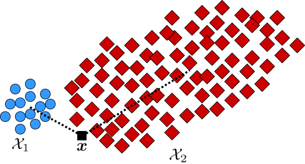
Remark 1 (Justification of the Mahalanobis distance (De Maesschalck et al., 2000)).
Consider two clouds of data, and , depicted in Fig. 1. We want to compute the distance of a point from these two data clouds to see which cloud this point is closer to. The Euclidean distance ignores the scatter/variance of clouds and only measures the distances of the point from the means of clouds. Hence, in this example, it says that belongs to because it is closer to the mean of compared to . However, the Mahalanobis distance takes the variance of clouds into account and says that belongs to because it is closer to its scatter compared to . Visually, human also says belongs to ; hence, the Mahalanobis distance has performed better than the Euclidean distance by considering the variances of data.
2.3 Generalized Mahalanobis Distance
Definition 3 (Generalized Mahalanobis distance).
In Mahalanobis distance, i.e. Eq. (2), the covariance matrix and its inverse are positive semi-definite. We can replace with a positive semi-definite weight matrix in the squared Mahalanobis distance. We name this distance a generalized Mahalanobis distance:
| (5) | ||||
We define the generalized Mahalanobis norm as:
| (6) |
Lemma 1 (Triangle inequality of norm).
Let be a norm. Using the Cauchy-Schwarz inequality, it satisfies the triangle inequality:
| (7) |
Proof.
where is because of the Cauchy-Schwarz inequality, i.e., . Taking second root from the sides gives Eq. (7). Q.E.D. ∎
Proposition 1.
The generalized Mahalanobis distance is a valid distance metric.
Proof.
Remark 2.
It is noteworthy that is required so that the generalized Mahalanobis distance is convex and satisfies the triangle inequality.
Remark 3.
The weight matrix in Eq. (5) weights the dimensions and determines some correlation between dimensions of data points. In other words, it changes the space in a way that the scatters of clouds are considered.
Remark 4.
Proposition 2 (Projection in metric learning).
Consider the eigenvalue decomposition of the weight matrix in the generalized Mahalanobis distance with and as the matrix of eigenvectors and the diagonal matrix of eigenvalues of the weight, respectively. Let . The generalized Mahalanobis distance can be seen as the Euclidean distance after applying a linear projection onto the column space of :
| (8) | ||||
If with , the column space of the projection matrix is a -dimensional subspace.
Proof.
By the eigenvalue decomposition of , we have:
| (9) |
where is because is positive semi-definite so all its eigenvalues are non-negative and can be written as multiplication of its second roots. Also, is because we define . Substituting Eq. (9) in Eq. (5) gives:
Q.E.D. It is noteworthy that Eq. (9) can also be obtained using singular value decomposition rather than eigenvalue decomposition. In that case, the matrices of right and left singular vectors are equal because of symmetry of . ∎
2.4 The Main Idea of Metric Learning
Consider a -dimensional dataset of size . Assume some data points are similar in some sense. For example, they have similar pattern or the same characteristics. Hence, we have a set of similar pair points, denotes by . In contrast, we can have dissimilar points which are different in pattern or characteristics. Let the set of dissimilar pair points be denoted by . In summary:
| (10) | ||||
The measure of similarity and dissimilarity can be belonging to the same or different classes, if class labels are available for dataset. In this case, we have:
| (11) | ||||
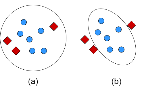
In metric learning, we learn the weight matrix so that the distances of similar points become smaller and the distances of dissimilar points become larger. In this way, the variance of similar and dissimilar points get smaller and larger, respectively. A 2D visualization of metric learning is depicted in Fig. 2. If the class labels are available, metric learning tries to make the intra-class and inter-class variances smaller and larger, respectively. This is the same idea as the idea of Fisher Discriminant Analysis (FDA) (Fisher, 1936; Ghojogh et al., 2019b).
3 Spectral Metric Learning
3.1 Spectral Methods Using Scatters
3.1.1 The First Spectral Method
The first metric learning method was proposed in (Xing et al., 2002). In this method, we minimize the distances of the similar points by the weight matrix where this matrix is positive semi-definite:
| subject to |
However, the solution of this optimization problem is trivial, i.e., . Hence, we add a constraint on the dissimilar points to have distances larger than some positive amount:
| (12) | ||||||
| subject to | ||||||
where is some positive number such as .
Lemma 2 ((Xing et al., 2002)).
If the constraint in Eq. (12) is squared, i.e., , the solution of optimization will have rank . Hence, we are using a non-squared constraint in the optimization problem.
Proof.
If the constraint in Eq. (12) is squared, the problem is equivalent to (see (Ghojogh et al., 2019b, Appendix B) for proof):
which is a Rayleigh-Ritz quotient (Ghojogh et al., 2019a). We can restate as:
| (13) | |||
where denotes the trace of matrix and:
| (14) | |||
Hence, we have:
where is because of the cyclic property of trace and is because . Maximizing this Rayleigh-Ritz quotient results in the following generalized eigenvalue problem (Ghojogh et al., 2019a):
where is the eigenvector with largest eigenvalue and the other eigenvectors are zero vectors. Q.E.D. ∎
The Eq. (12) can be restated as a maximization problem:
| (15) | ||||||
| subject to | ||||||
We can solve this problem using projected gradient method (Ghojogh et al., 2021c) where a step of gradient ascent is followed by projection onto the two constraint sets:
where is the learning rate and and are the eigenvectors and eigenvalues of , respectively (see Eq. (9)).
3.1.2 Formulating as Semidefinite Programming
Another metric learning method is (Ghodsi et al., 2007) which minimizes the distances of similar points and maximizes the distances of dissimilar points. For this, we minimize the distances of similar points and the negation of distances of dissimilar points. The weight matrix should be positive semi-definite to satisfy the triangle inequality and convexity. The trace of weight matrix is also set to a constant to eliminate the trivial solution . The optimization problem is:
| (16) | ||||||
| subject to | ||||||
where denotes the cardinality of set.
Lemma 3 ((Ghodsi et al., 2007)).
The objective function can be simplified as:
| (17) | ||||
where vectorizes the matrix to a vector (Ghojogh et al., 2021c).
Proof.
See (Ghodsi et al., 2007, Section 2.1) for proof. ∎
3.1.3 Relevant to Fisher Discriminant Analysis
Another metric learning method is (Alipanahi et al., 2008) which has two approaches, introduced in the following. The relation of metric learning with Fisher discriminant analysis (Fisher, 1936; Ghojogh et al., 2019b) was discussed in this paper (Alipanahi et al., 2008).
– Approach 1: As , the weight matrix can be decomposed as in Eq. (9), i.e., . Hence, we have:
| (18) |
where is because a scalar is equal to its trace and is because of the cyclic property of trace. We can substitute Eq. (18) in Eq. (16) to obtain an optimization problem:
| (19) | ||||||
| subject to | ||||||
whose objective variable is . Note that the constraint is implicitly satisfied because of the decomposition . We define:
| (20) | ||||
Hence, Eq. (19) can be restated as:
| (21) | ||||||
| subject to |
whose Lagrangian is (Ghojogh et al., 2021c):
Taking derivative of the Lagrangian and setting it to zero gives:
| (22) |
which is the eigenvalue problem for (Ghojogh et al., 2019a). Hence, is the eigenvector of with the smallest eigenvalue because Eq. (19) is a minimization problem.
– Approach 2: We can change the constraint in Eq. (21) to have orthogonal projection matrix, i.e., . Rather, we can make the rotation of the projection matrix by the matrix be orthogonal, i.e., . Hence, the optimization problem becomes:
| (23) | ||||||
| subject to |
whose Lagrangian is (Ghojogh et al., 2021c):
| (24) |
which is the generalized eigenvalue problem for (Ghojogh et al., 2019a). Hence, is a matrix whose columns are the eigenvectors sorted from the smallest to largest eigenvalues.
The optimization problem is similar to the optimization of Fisher discriminant analysis (FDA) (Fisher, 1936; Ghojogh et al., 2019b) where and are replaced with the intra-class and inter-class covariance matrices of data, respectively. This shows the relation of this method with FDA. It makes sense because both metric learning and FDA have the same goal and that is decreasing and increasing the variances of similar and dissimilar points, respectively.
3.1.4 Relevant Component Analysis (RCA)
Suppose the data points can be divided into clusters, or so-called chunklets. If class labels are available, classes are the chunklets. If denotes the data of the -th cluster and is the mean of , the summation of intra-cluster scatters is:
| (25) |
Relevant Component Analysis (RCA) (Shental et al., 2002) is a metric learning method. In this method, we first apply Principal Component Analysis (PCA) (Ghojogh & Crowley, 2019) on data using the total scatter of data. Let the projection matrix of PCA be denoted by . After projection onto the PCA subspace, the summation of intra-cluster scatters is because of the quadratic characteristic of covariance. RCA uses as the covariance matrix in the Mahalanobis distance, i.e., Eq. (2). According to Eq. (8), the subspace of RDA is obtained by the eigenvalue (or singular value) decomposition of (see Eq. (9)).
3.1.5 Discriminative Component Analysis (DCA)
Discriminative Component Analysis (DCA) (Hoi et al., 2006) is another spectral metric learning method based on scatters of clusters/classes. Consider the clusters, chunklets, or classes of data. The intra-class scatter is as in Eq. (25). The inter-class scatter is:
| (26) | ||||
where is the mean of the -th class and is the total mean of data. According to Proposition 2, metric learning can be seen as Euclidean distance after projection onto the column space of a projection matrix where . Similar to Fisher discriminant analysis (Fisher, 1936; Ghojogh et al., 2019b), DCA maximizes the inter-class variance and minimizes the intra-class variance after projection. Hence, its optimization is:
| (27) |
which is a generalized Rayleigh-Ritz quotient. The solution to this optimization problem is the generalized eigenvalue problem (Ghojogh et al., 2019a). According to Eq. (9), we can set the weight matrix of the generalized Mahalanobis distance as where is the matrix of eigenvectors.
3.1.6 High Dimensional Discriminative Component Analysis
Another spectral method for metric learning is (Xiang et al., 2008) which minimizes and maximizes the intra-class and inter-class variances, respectively, by the the same optimization problem as Eq. (27) with an additional constraint on the orthogonality of the projection matrix, i.e., . This problem can be restated by posing penalty on the denominator:
| (28) | ||||||
| subject to |
where is the regularization parameter. The solution to this problem is the eigenvalue problem for . The eigenvectors are the columns of and the weight matrix of the generalized Mahalanobis is obtained using Eq. (9).
If the dimensionality of data is large, computing the eigenvectors of is very time-consuming. According to (Xiang et al., 2008, Theorem 3), the optimization problem (28) can be solved in the orthogonal complement space of the null space of without loss of any information (see (Xiang et al., 2008, Appendix A) for proof). Hence, if , we find as follows. Let be the matrix of data. Let and be the adjacency matrices for the sets and , respectively. For example, if , then ; otherwise, . If and are the Laplacian matrices of and , respectively, we have and (see (Belkin & Niyogi, 2002; Ghojogh et al., 2021d) for proof). We have because of the cyclic property of trace. If the rank of is , it has non-zero eigenvalues which we compute its corresponding eigenvectors. We stack these eigenvectors to have . The projected intra-class and inter-class variances after projection onto the column space of are and , respectively. Then, we use and in Eq. (28) and the weight matrix of the generalized Mahalanobis is obtained using Eq. (9).
3.1.7 Regularization by Locally Linear Embedding
The spectral metric learning methods using scatters can be modeled as maximization of the following Rayleigh–Ritz quotient (Baghshah & Shouraki, 2009):
| (29) | ||||||
| subject to |
where (see Eq. (9)), is the regularization parameter, and is a penalty or regularization term on the projection matrix . This optimization maximizes and minimizes the distances of the similar and dissimilar points, respectively. According to Section 3.1.3, Eq. (29) can be restated as:
| (30) | ||||||
| subject to |
As was discussed in Proposition 2, metric learning can be seen as projection onto a subspace. The regularization term can be linear reconstruction of every projected point by its Nearest Neighbors (NN) using the same reconstruction weights as before projection (Baghshah & Shouraki, 2009). The weights for linear reconstruction in the input space can be found as in locally linear embedding (Roweis & Saul, 2000; Ghojogh et al., 2020a). If denotes the weight of in reconstruction of and is the set of NN for , we have:
| subject to |
The solution of this optimization is (Ghojogh et al., 2020a):
where in which denotes the stack of NN for . We define . The regularization term can be reconstruction in the subspace using the same reconstruction weights as in the input space (Baghshah & Shouraki, 2009):
| (31) |
where and . Putting Eq. (31) in Eq. (30) gives:
| (32) | ||||||
| subject to |
The solution to this optimization problem is the generalized eigenvalue problem where has the eigenvectors as its columns (Ghojogh et al., 2019a). According to Eq. (9), the weight matrix of metric is .
3.1.8 Fisher-HSIC Multi-view Metric Learning (FISH-MML)
Fisher-HSIC Multi-view Metric Learning (FISH-MML) (Zhang et al., 2018) is a metric learning method for multi-view data. In multi-view data, we have different types of features for every data point. For example, an image dataset, which has a descriptive caption for every image, is multi-view. Let be the features of data points in the -th view, be the number of classes/clusters, and be the number of views. According to Proposition 2, metric learning is the Euclidean distance after projection with . The inter-class scatter of data, in the -th view, is denoted by and calculated using Eqs. (26). The total scatter of data, in the -th view, is denoted by and is the covariance of data in that view.
Inspired by Fisher discriminant analysis (Fisher, 1936; Ghojogh et al., 2019b), we maximize the inter-class variances of projected data, , to discriminate the classes after projection. Also, inspired by principal component analysis (Ghojogh & Crowley, 2019), we maximize the total scatter of projected data, , for expressiveness. Moreover, we maximize the dependence of the projected data in all views because various views of a point should be related. A measure of dependence between two random variables and is the Hilbert-Schmidt Independence Criterion (HSIC) (Gretton et al., 2005) whose empirical estimation is:
| (33) |
where and are kernel matrices over and variables, respectively, and is the centering matrix. The HSIC between projection of two views and is:
where is because we use the linear kernel for , i.e., and is because of the cyclic property of trace.
In summary, we maximize the summation of inter-class scatter, total scatter, and the dependence of views, which is:
where are the regularization parameters. The optimization problem is:
| (34) | ||||||
| subject to | ||||||
whose solution is the eigenvalue problem for where has the eigenvectors as its columns (Ghojogh et al., 2019a).
3.2 Spectral Methods Using Hinge Loss
3.2.1 Large-Margin Metric Learning
-Nearest Neighbors (NN) classification is highly impacted by the metric used for measuring distances between points. Hence, we can use metric learning for improving the performance of NN classification (Weinberger et al., 2006; Weinberger & Saul, 2009). Let if and if . Moreover, we consider NN for similar points where we find the nearest neighbors of every point among the similar points to that point. Let if and is among NN of . Otherwise, . The optimization problem for finding the best weigh matrix in the metric can be (Weinberger et al., 2006; Weinberger & Saul, 2009):
| (35) | ||||||
| subject to | ||||||
where is the regularization parameter, and is the standard Hinge loss.
The first term in Eq. (35) pushes the similar neighbors close to each other. The second term in this equation is the triplet loss (Schroff et al., 2015) which pushes the similar neighbors to each other and pulls the dissimilar points away from one another. This is because minimizing for decreases the distances of similar neighbors. Moreover, minimizing for (i.e., ) is equivalent to maximizing which maximizes the distances of dissimilar points. Minimizing the whole second term forces the distances of dissimilar points to be at least greater that the distances of similar points up to a threshold (or margin) of one. We can change the margin by changing in this term with some other positive number. In this sense, this loss is closely related to the triplet loss for neural networks (Schroff et al., 2015) (see Section 5.3.5).
Eq. (35) can be restated using slack variables . The Hinge loss in term requires to have:
If , we can have sandwich the term in order to minimize it:
Hence, we can replace the term of Hinge loss with the slack variable. Therefore, Eq. (35) can be restated as (Weinberger et al., 2006; Weinberger & Saul, 2009):
| (36) | ||||||
| subject to | ||||||
This optimization problem is a semidefinite programming which can be solved iteratively using interior-point method (Ghojogh et al., 2021c).
This problem uses triplets of similar and dissimilar points, i.e., where , , . Hence, triplets should be extracted randomly from the dataset for this metric learning. Solving semidefinite programming is usually slow and time-consuming especially for large datasets. Triplet minimizing can be used for finding the best triplets for learning (Poorheravi et al., 2020). For example, the similar and dissimilar points with smallest and/or largest distances can be used to limit the number of triplets (Sikaroudi et al., 2020a). The reader can also refer to for Lipschitz analysis in large margin metric learning (Dong, 2019).
3.2.2 Imbalanced Metric Learning (IML)
Imbalanced Metric Learning (IML) (Gautheron et al., 2019) is a spectral metric learning method which handles imbalanced classes by further decomposition of the similar set and dissimilar set . Suppose the dataset is composed of two classes and . Let and denote the similarity sets for classes and , respectively. We define pairs of points taken randomly from these sets to have similarity and dissimilarity sets (Gautheron et al., 2019):
The optimization problem of IML is:
| (37) |
where denotes the cardinality of set, is the standard Hinge loss, is the desired margin between classes, and and are the regularization parameters. This optimization pulls the similar points to have distance less than and pushes the dissimilar points away to have distance more than . Also, the regularization term tries to make the weight matrix is the generalized Mahalanobis distance close to identity for simplicity of metric. In this way, the metric becomes close to the Euclidean distance, preventing overfitting, while satisfying the desired margins in distances.
3.3 Locally Linear Metric Adaptation (LLMA)
Another method for metric learning is Locally Linear Metric Adaptation (LLMA) (Chang & Yeung, 2004). LLMA performs nonlinear and linear transformations globally and locally, respectively. For every point , we consider its nearest (similar) neighbors. The local linear transformation for every point is:
| (38) |
where is the matrix of biases, , and is a Gaussian measure of similarity between and . The variables and are found by optimization.
In this method, we minimize the distances between the linearly transformed similar points while the distances of similar points are tried to be preserved after the transformation:
| (39) | ||||||
where is the regularization parameter, is the variance to be optimized, and and . This objective function is optimized iteratively until convergence.
3.4 Relevant to Support Vector Machine
Inspired by -Support Vector Machine (-SVM) (Schölkopf et al., 2000), the weight matrix in the generalized Mahalanobis distance can be obtained as (Tsang et al., 2003):
| (40) | ||||||
| subject to | ||||||
where are regularization parameters. Using KKT conditions and Lagrange multipliers (Ghojogh et al., 2021c), the dual optimization problem is (see (Tsang et al., 2003) for derivation):
| (41) | ||||
where are the dual variables. This problem is a quadratic programming problem and can be solved using optimization solvers.
3.5 Relevant to Multidimensional Scaling
Multidimensional Scaling (MDS) tries to preserve the distance after projection onto its subspace (Cox & Cox, 2008; Ghojogh et al., 2020b). We saw in Proposition 2 that metric learning can be seen as projection onto the column space of where . Inspired by MDS, we can learn a metric which preserves the distances between points after projection onto the subspace of metric (Zhang et al., 2003):
| (42) | ||||||
| subject to |
It can be solved using any optimization method (Ghojogh et al., 2021c).
3.6 Kernel Spectral Metric Learning
Let be the kernel function over data points and , where is the pulling function to the Reproducing Kernel Hilbert Space (RKHS) (Ghojogh et al., 2021e). Let be the kernel matrix of data. In the following, we introduce some of the kernel spectral metric learning methods.
3.6.1 Using Eigenvalue Decomposition of Kernel
One of the kernel methods for spectral metric learning is (Yeung & Chang, 2007). It has two approaches; we explain one of its approaches here. The eigenvalue decomposition of the kernel matrix is:
| (43) |
where is the rank of kernel matrix, is the non-negative -th eigenvalue (because ), is the -th eigenvector, and is because we define . We can consider as learnable parameters and not the eigenvalues. Hence, we learn for the sake of metric learning. The distance metric of pulled data points to RKHS is (Schölkopf, 2001; Ghojogh et al., 2021e):
| (44) | ||||
In metric learning, we want to make the distances of similar points small; hence the objective to be minimized is: Hence, we have:
where is because is the vector whose -th element is one and other elements are zero, is because we define , and is because we define and . By adding a constraint on the summation of , the optimization problem for metric learning is:
| (45) | ||||||
| subject to |
This optimization is similar to the form of one of the optimization problems in locally linear embedding (Roweis & Saul, 2000; Ghojogh et al., 2020a). The Lagrangian for this problem is (Ghojogh et al., 2021c):
where is the dual variable. Taking derivative of the Lagrangian w.r.t. the variables and setting to zero gives:
Hence, the optimal is obtained for metric learning in the RKHS where the distances of similar points is smaller than in the input Euclidean space.
3.6.2 Regularization by Locally Linear Embedding
The method (Baghshah & Shouraki, 2009), which was introduced in Section 3.1.7, can be kernelized. Recall that this method used locally linear embedding for regularization. According to the representation theory (Ghojogh et al., 2021e), the solution in the RKHS can be represented as a linear combination of all pulled data points to RKHS:
| (46) |
where and ( is the dimensionality of subspace) is the coefficients.
We define the similarity and dissimilarity adjacency matrices as:
| (47) | ||||
Let and denote the Laplacian matrices (Ghojogh et al., 2021d) of these adjacency matrices:
where and are diagonal matrices. The terms in the objective of Eq. (32) can be restated using Laplacian of adjacency matrices rather than the scatters:
| (48) | ||||||
| subject to |
According to the representation theory, the pulled Laplacian matrices to RKHS are and . Hence, the numerator of Eq. (32) in RKHS becomes:
where is because of the kernel trick (Ghojogh et al., 2021e), i.e.,
| (49) |
similarly, the denominator of Eq. (32) in RKHS becomes:
where is because of the kernel trick (Ghojogh et al., 2021e). The constrain in RKHS becomes:
where is because of the kernel trick (Ghojogh et al., 2021e). The Eq. (32) in RKHS is:
| (50) | ||||||
| subject to |
It can be solved using projected gradient method (Ghojogh et al., 2021c) to find the optimal . Then, the projected data onto the subspace of metric is found as:
| (51) |
where is because of the kernel trick (Ghojogh et al., 2021e).
3.6.3 Regularization by Laplacian
Another kernel spectral metric learning method is (Baghshah & Shouraki, 2010) whose optimization is in the form:
| (52) | ||||||
| subject to |
where is a hyperparameter and is the regularization parameter. Consider the NN graph of data with an adjacency matrix whose -th element is one if and are neighbors and is zero otherwise. Let the Laplacian matrix of this adjacency matrix be denoted by .
In this method, the regularization term can be the objective of Laplacian eigenmap (Ghojogh et al., 2021d):
where is according to (Belkin & Niyogi, 2001) (see (Ghojogh et al., 2021d) for proof), is because of the cyclic property of trace, and is because of the kernel trick (Ghojogh et al., 2021e). Moreover, according to Eq. (44), the distance in RKHS is . We can simplify the term in Eq. (52) as:
where is because the scalar is equal to its trace and we use the cyclic property of trace, i.e., , and then we define .
Hence, Eq. (52) can be restated as:
| (53) | ||||||
| subject to | ||||||
noticing that the kernel matrix is positive semidefinite. This problem is a Semidefinite Programming (SDP) problem and can be solved using the interior point method (Ghojogh et al., 2021c). The optimal kernel matrix can be decomposed using eigenvalue decomposition to find the embedding of data in RKHS, i.e., :
where and are the eigenvectors and eigenvalues, is because so its eigenvalues are non-negative can be taken second root of, and is because we get .
3.6.4 Kernel Discriminative Component Analysis
Here, we explain the kernel version of DCA (Hoi et al., 2006) which was introduced in Section 3.1.5.
Lemma 4.
The generalized Mahalanobis distance metric in RKHS, with the pulled weight matrix to RKHS denoted by , can be seen as measuring the Euclidean distance in RKHS after projection onto the column subspace of where is the coefficient matrix in Eq. (46). In other words:
| (54) | ||||
where is the kernel vector between and .
Proof.
We can have the decomposition of the weight matrix, i.e. Eq. (9), in RKHS which is:
| (55) |
The generalized Mahalanobis distance metric in RKHS is:
where is because of the kernel trick, i.e., . Q.E.D. ∎
Let where denotes the cardinality of the -th class. Let and be the kernelized versions of and , respectively (see Eqs. (25) and (26)). If denotes the -th class, we have:
| (56) | |||
| (57) |
We saw the metric in RKHS can be seen as projection onto a subspace with the projection matrix . Therefore, Eq. (27) in RKHS becomes (Hoi et al., 2006):
| (58) |
which is a generalized Rayleigh-Ritz quotient. The solution to this optimization problem is the generalized eigenvalue problem (Ghojogh et al., 2019a). The weight matrix of the generalized Mahalanobis distance is obtained by Eqs. (46) and (55).
3.6.5 Relevant to Kernel Fisher Discriminant Analysis
Here, we explain the kernel version of the metric learning method (Alipanahi et al., 2008) which was introduced in Section 3.1.3.
According to Eq. (54), we have:
where is because a scalar it equal to its trace and is because of the cyclic property of trace. Hence, Eq. (20) in RKHS becomes:
and likewise:
where:
Hence, in RKHS, the objective of the optimization problem (23) becomes . We change the constraint in Eq. (23) to . In RKHS, this constraint becomes:
Finally, (23) in RKHS becomes:
| (59) | ||||||
| subject to |
whose solution is a generalized eigenvalue problem where is the matrix of eigenvectors. The weight matrix of the generalized Mahalanobis distance is obtained by Eqs. (46) and (55). This is relevant to kernel Fisher discriminant analysis (Mika et al., 1999; Ghojogh et al., 2019b) which minimizes and maximizes the intra-class and inter-class variances in RKHS.
3.6.6 Relevant to Kernel Support Vector Machine
Here, we explain the kernel version of the metric learning method (Tsang et al., 2003) which was introduced in Section 3.4. It is relevant to kernel SVM. Using kernel trick (Ghojogh et al., 2021e) and Eq. (54), the Eq. (41) can be kernelized as (Tsang et al., 2003):
| (60) | ||||
which is a quadratic programming problem and can be solved by optimization solvers.
3.7 Geometric Spectral Metric Learning
Some spectral metric learning methods are geometric methods which use Riemannian manifolds. In the following, we introduce the mist well-known geometric methods. There are some other geometric methods, such as (Hauberg et al., 2012), which are not covered for brevity.
3.7.1 Geometric Mean Metric Learning
One of the geometric spectral metric learning is Geometric Mean Metric Learning (GMML) (Zadeh et al., 2016). Let be the weight matrix in the generalized Mahalanobis distance for similar points.
– Regular GMML: In GMML, we use the inverse of weight matrix, i.e. , for the dissimilar points. The optimization problem of GMML is (Zadeh et al., 2016):
| (61) | ||||||
| subject to | ||||||
According to Eq. (13), this problem can be restated as:
| (62) | ||||||
| subject to |
where and are defined in Eq. (14). Taking derivative of the objective function w.r.t. and setting it to zero gives:
| (63) |
This equation is the Riccati equation (Riccati, 1724) and its solution is the midpoint of the geodesic connecting and (Bhatia, 2007, Section 1.2.13).
Lemma 5 ((Bhatia, 2007, Chapter 6)).
The geodesic curve connecting two points and on the Symmetric Positive Definite (SPD) Riemannian manifold is denoted by and is computed as:
| (64) |
where .
Hence, the solution of Eq. (63) is:
| (65) |
The proof of Eq. (65) is as follows (Hajiabadi et al., 2019):
where is because so its eigenvalues are non-negative and the matrix of eigenvalues can be decomposed by the second root in its eigenvalue decomposition to have .
– Regularized GMML: The matrix might be singular or near singular and hence non-invertible. Therefore, we regularize Eq. (62) to make the weight matrix close to a prior known positive definite matrix .
| (66) | ||||||
| subject to | ||||||
where is the regularization parameter. The regularization term is the symmetrized log-determinant divergence between and . Taking derivative of the objective function w.r.t. and setting it to zero gives:
which is again a Riccati equation (Riccati, 1724) whose solution is the midpoint of the geodesic connecting and :
| (67) |
– Weighted GMML: Eq. (62) can be restated as:
| (68) | ||||||
| subject to |
where is the Riemannian distance (or Fréchet mean) on the SPD manifold (Arsigny et al., 2007, Eq 1.1):
where is the Frobenius norm. We can weight the objective in Eq. (68):
| (69) | ||||||
| subject to |
where is a hyperparameter. The solution of this problem is the weighted version of Eq. (67):
| (70) |
3.7.2 Low-rank Geometric Mean Metric Learning
We can learn a low-rank weight matrix in GMML (Bhutani et al., 2018), where the rank of wight matrix is set to be :
| (71) | ||||||
| subject to | ||||||
We can decompose it using eigenvalue decomposition as done in Eq. (9), i.e., , where we only have eigenvectors and eigenvalues. Therefore, the sizes of matrices are , , and . By this decomposition, the objective function in Eq. (71 can be restated as:
where because it is orthogonal, is because of the cyclic property of trace, and is because we define and . Noticing that the matrix of eigenvectors is orthogonal, the Eq. (71) is restated to:
| (72) | ||||||
| subject to | ||||||
where is automatically satisfied by taking and in the decomposition. This problem can be solved by the alternative optimization (Ghojogh et al., 2021c). If the variable is fixed, minimization w.r.t. is similar to the problem (62); hence, its solution is similar to Eq. (65), i.e., (see Eq. (64) for the definition of ). If is fixed, the orthogonality constraint can be modeled by belonging to the Grassmannian manifold which is the set of -dimensional subspaces of . To sum up, the alternative optimization is:
where is the iteration index. Optimization of can be solved by Riemannian optimization (Absil et al., 2009).
3.7.3 Geometric Mean Metric Learning for Partial Labels
Partial label learning (Cour et al., 2011) refers to when a set of candidate labels is available for every data point. GMML can be modified to be used for partial label learning (Zhou & Gu, 2018). Let denote the set of candidate labels for . If there are candidate labels in total, we denote where is one if the -th label is a candidate label for and is zero otherwise. We define and . In other words, and are the data points which share and do not share some candidate labels with , respectively. Let be the indices of the nearest neighbors of among . Also, let be the indices of points in whose distance from are smaller than the distance of the furthest point in from . In other words, .
Let contain the probabilities that each of the neighbors of share the same label with . It can be estimated by linear reconstruction of by the neighbor ’s:
| subject to |
where is the regularization parameter. Let denote the coefficients for linear reconstruction of by its nearest neighbors. It is obtained as:
| subject to |
These two optimization problems are quadratic programming and can be solved using the interior point method (Ghojogh et al., 2021c).
The main optimization problem of GMML for partial labels is (Zhou & Gu, 2018):
| (73) | ||||||
| subject to |
where:
Minimizing the first term of in decreases the distances of similar points which share some candidate labels. Minimizing the second term of in tries to preserve linear reconstruction of by its neighbors after projection onto the subspace of metric. Minimizing increases the the distances of dissimilar points which do not share any candidate labels. The problem (73) is similar to the problem (62); hence, its solution is similar to Eq. (65), i.e., (see Eq. (64) for the definition of ).
3.7.4 Geometric Mean Metric Learning on SPD and Grassmannian Manifolds
The GMML method (Zadeh et al., 2016), introduced in Section 3.7.1, can be implemented on Symmetric Positive Definite (SPD) and Grassmannian manifolds (Zhu et al., 2018). If is a point on the SPD manifold, the distance metric on this manifold is (Zhu et al., 2018):
| (74) |
where is the weight matrix of metric and is the logarithm operation on the SPD manifold. The Grassmannian manifold is the -dimensional subspaces of the -dimensional vector space. A point in is a linear subspace spanned by a full-rank which is orthogonal, i.e., . If is any matrix, We define in a way that is the orthogonal components of . If , the distance on the Grassmannian manifold is (Zhu et al., 2018):
| (75) |
is the weight matrix of metric.
Similar to the optimization problem of GMML, i.e. Eq. (61), we solve the following problem for the SPD manifold:
| (76) | ||||||
| subject to | ||||||
Likewise, for the Grassmannian manifold, the optimization problem is:
| (77) | ||||||
| subject to | ||||||
Suppose, for the SPD manifold, we define:
and, for the Grassmannian manifold, we define:
Hence, for either SPD or Grassmannian manifold, the optimization problem becomes Eq. (62) in which and are replaced with and , respectively.
3.7.5 Metric Learning on Stiefel and SPD Manifolds
According to Eq. (9), the weight matrix in the metric can be decomposed as . If we do not restrict and to be the matrices of eigenvectors and eigenvalues as in Eq. (9), we can learn both and by optimization (Harandi et al., 2017). The optimization problem in this method is:
| (78) | ||||||
| subject to | ||||||
where is the regularization parameter, denotes the determinant of matrix, and models Gaussian distribution with the generalized Mahalanobis distance metric:
The constraint means that the matrix belongs to the Stiefel manifold and the constraint means belongs to the SPD manifold . Hence, these two variables belong to the product manifold . Hence, we can solve this optimization problem using Riemannian optimization methods (Absil et al., 2009). This method can also be kernelized; the reader can refer to (Harandi et al., 2017, Section 4) for its kernel version.
3.7.6 Curvilinear Distance Metric Learning (CDML)
Lemma 6 ((Chen et al., 2019)).
The generalized Mahalanobis distance can be restated as:
| (79) |
where is the -th column of in Eq. (9), , and is the projection of satisfying .
Proof.
where is because of the law of cosines and is because of . The distance can be replaced by the length of the arc between and on the straight line for . This gives the Eq. (79). Q.E.D. ∎
The condition is equivalent to finding the nearest neighbor to the line , i.e., (Chen et al., 2019). This equation can be generalized to find the nearest neighbor to the geodesic curve rather than the line :
| (80) |
Hence, we can replace the arc length of the straight line in Eq. (79) with the arc length of the curve:
| (81) |
where is derivative of w.r.t. and is the scale factor. The Curvilinear Distance Metric Learning (CDML) (Chen et al., 2019) uses this approximation of distance metric by the above curvy geodesic on manifold, i.e., Eq. (81). The optimization problem in CDML is:
| (82) |
where is the number of points, , if and if , is defined in Eq. (81), is the regularization parameter, is some loss function, and is some penalty term. The optimal , obtained from Eq. (82), can be used in Eq. (81) to have the optimal distance metric. A recent follow-up of CDML is (Zhang et al., 2021).
3.8 Adversarial Metric Learning (AML)
Adversarial Metric Learning (AML) (Chen et al., 2018) uses adversarial learning (Goodfellow et al., 2014; Ghojogh et al., 2021b) for metric learning. On one hand, we have a distinguishment stage which tries to discriminate the dissimilar points and push similar points close to one another. On the other hand, we have an confusion or adversarial stage which tries to fool the metric learning method by pulling the dissimilar points close to each other and pushing the similar points away. The distinguishment and confusion stages are trained simultaneously and they make each other stronger gradually.
From the dataset, we form random pairs . If and are similar points, we set and if they are dissimilar, we have . We also generate some random new points in pairs . The generated points are updated iteratively by optimization of the confusion stage to fool the metric. The loss functions for both stages are Eq. (61) used in geometric mean metric learning (see Section 3.7.1).
The alternative optimization (Ghojogh et al., 2021c) used in AML is:
| (83) | ||||
until convergence, where are the regularization parameters. Updating and are the distinguishment and confusion stages, respectively. In the distinguishment stage, we find a weight matrix to minimize the distances of similar points in both and and maximize the distances of dissimilar points in both and . In the confusion stage, we generate new points to adversarially maximize the distances of similar points in and adversarially minimize the distances of dissimilar points in . In this stage, we also make the points and similar to their corresponding points and , respectively.
4 Probabilistic Metric Learning
Probabilistic methods for metric learning learn the weight matrix in the generalized Mahalanobis distance using probability distributions. They define some probability distribution for each point accepting other points as its neighbors. Of course, the closer points have higher probability for being neighbors.
4.1 Collapsing Classes
One probabilistic method for metric learning is collapsing similar points to the same class while pushing the dissimilar points away from one another (Globerson & Roweis, 2005). The probability distribution between points for being neighbors can be a Gaussian distribution which uses the generalized Mahalanobis distance as its metric. The distribution for to take as its neighbor is (Goldberger et al., 2005):
| (84) |
where we define the normalization factor, also called the partition function, as . This factor makes the summation of distribution one. Eq. (84) is a Gaussian distribution whose covariance matrix is because it is equivalent to:
We want the similar points to collapse to the same point after projection onto the subspace of metric (see Proposition 2). Hence, we define the desired neighborhood distribution to be a bi-level distribution (Globerson & Roweis, 2005):
| (87) |
This makes all similar points of a group/class a same point after projection.
4.1.1 Collapsing Classes in the Input Space
For making close to the desired distribution , we minimize the KL-divergence between them (Globerson & Roweis, 2005):
| (88) | ||||||
| subject to |
Lemma 7 ((Globerson & Roweis, 2005)).
Let the the objective function in Eq. (88) be denoted by . The gradient of this function w.r.t. is:
| (89) |
Proof.
The derivation is similar to the derivation of gradient in Stochastic Neighbor Embedding (SNE) and t-SNE (Hinton & Roweis, 2003; van der Maaten & Hinton, 2008; Ghojogh et al., 2020c). Let:
| (90) |
By changing , we only have change impact in and (or and ) for all ’s. According to chain rule, we have:
According to Eq. (90), we have:
where is because of the cyclic property of trace. Therefore:
| (91) |
The dummy variables in cost function can be re-written as:
whose first term is a constant with respect to and thus to . We have:
According to Eqs. (84) and (90), the is:
We take the denominator of as:
| (92) |
We have . Therefore:
The is:
Therefore, we have:
The is non-zero for only and ; therefore:
Therefore:
We have because summation of all possible probabilities is one. Thus:
| (93) |
Substituting the obtained derivative in Eq. (91) gives Eq. (89). Q.E.D. ∎
The optimization problem (88) is convex; hence, it has a unique solution. We can solve it using any optimization method such as the projected gradient method, where after every gradient descent step, we project the solution onto the positive semi-definite cone (Ghojogh et al., 2021c):
where is the learning rate and and are the eigenvectors and eigenvalues of , respectively (see Eq. (9)).
4.1.2 Collapsing Classes in the Feature Space
According to Eq. (54), the distance in the feature space can be stated using kernels as where is the kernel vector between dataset and the point . We define . Hence, in the feature space, Eq. (84) becomes:
| (94) |
The gradient in Eq. (89) becomes:
| (95) |
Again, we can find the optimal using projected gradient method. This gives us the optimal metric for collapsing classes in the feature space (Globerson & Roweis, 2005). Note that we can also regularize the objective function, using the trace operator or Frobenius norm, for avoiding overfitting.
4.2 Neighborhood Component Analysis Methods
Neighborhood Component Analysis (NCA) is one of the most well-known probabilistic metric learning methods. In the following, we introduce different variants of NCA.
4.2.1 Neighborhood Component Analysis (NCA)
In the original NCA (Goldberger et al., 2005), the probability that takes as its neighbor is as in Eq. (84), where we assume by convention:
| (98) |
Consider the decomposition of the weight matrix of metric as in Eq. (9), i.e., . Let denote the set of similar points to where . The optimization problem of NCA is to find a to maximize this probability distribution for similar points (Goldberger et al., 2005):
| (99) |
where:
| (100) |
Note that the required constraint is already satisfied because of the decomposition in Eq. (84).
Lemma 8 ((Goldberger et al., 2005)).
Suppose the objective function of Eq. (99) is denoted by . The gradient of this cost function w.r.t. is:
| (101) | ||||
The derivation of this gradient is similar to the approach in the proof of Lemma 7. We can use gradient ascent for solving the optimization.
Another approach is to maximize the log-likelihood of neighborhood probability (Goldberger et al., 2005):
| (102) |
whose gradient is (Goldberger et al., 2005):
| (103) | ||||
Again, gradient ascent can give us the optimal . As explained in Proposition 2, the subspace is metric is the column space of and projection of points onto this subspace reduces the dimensionality of data.
4.2.2 Regularized Neighborhood Component Analysis
It is shown by some experiments that NCA can overfit to training data for high-dimensional data (Yang & Laaksonen, 2007). Hence, we can regularize it to avoid overfitting. In regularized NCA (Yang & Laaksonen, 2007), we use the log-posterior of the matrix which is equal to:
| (104) |
according to the Bayes’ rule. We can use Gaussian distribution for the prior:
| (105) |
where is a constant factor including the normalization factor, is the inverse of variance, and is the -th element of . Note that we can have if we truncate it to have leading eigenvectors of (see Eq. (9)). The likelihood
| (106) |
The regularized NCA maximizes the log-posterior (Yang & Laaksonen, 2007):
where is because of Eqs. (105) and (106) and denotes the Frobenius norm. Hence, the optimization problem of regularized NCA is (Yang & Laaksonen, 2007):
| (107) |
where can be seen as the regularization parameter. The gradient is similar to Eq. (101) but plus the derivative of the regularization term which is .
4.2.3 Fast Neighborhood Component Analysis
– Fast NCA: The fast NCA (Yang et al., 2012) accelerates NCA by using -Nearest Neighbors (NN) rather than using all points for computing the neighborhood distribution of every point. Let and denote the NN of among the similar points to (denoted by ) and dissimilar points (denoted by ), respectively. Fast NCA uses following probability distribution for to take as its neighbor (Yang et al., 2012):
| (110) |
The optimization problem of fast NCA is similar to Eq. (107):
| (111) |
where is Eq. (110) and is the matrix in the decomposition of (see Eq. (9)).
Lemma 9 ((Yang et al., 2012)).
Suppose the objective function of Eq. (111) is denoted by . The gradient of this cost function w.r.t. is:
| (112) | ||||
This is similar to Eq. (101). See (Yang et al., 2012) for the derivation. We can use gradient ascent for solving the optimization.
– Kernel Fast NCA: According to Eq. (54), the distance in the feature space is where is the kernel vector between dataset and the point . We can use this distance metric in Eq. (110) to have kernel fast NCA (Yang et al., 2012). Hence, the gradient of kernel fast NCA is similar to Eq. (112):
| (113) | ||||
Again, we can find the optimal using gradient ascent. Note that the same technique can be used to kernelize the original NCA.
4.3 Bayesian Metric Learning Methods
In this section, we introduce the Bayesian metric learning methods which use variational inference (Ghojogh et al., 2021a) for metric learning. In Bayesian metric learning, we learn a distribution for the distance metric between every two points; we sample the pairwise distances from these learned distributions.
First, we provide some definition required in these methods. According to Eq. (9), we can decompose the weight matrix in the metric using the eigenvalue decomposition. Accordingly, we can approximate this matrix by:
| (114) |
where contains the eigenvectors of and is the diagonal matrix of eigenvalues which we learn in Bayesian metric learning. Let and denote the random variables for data and labels, respectively, and let denote the learnable eigenvalues. Let denote the -th column of . We define . The reader should not confuse with which is the weight matrix of metric in out notations.
4.3.1 Bayesian Metric Learning Using Sigmoid Function
One of the Bayesian metric learning methods is (Yang et al., 2007). We define:
| (117) |
We can consider a sigmoid function for the likelihood (Yang et al., 2007):
| (118) |
where is a threshold. We can also derive an evidence lower bound for ; we do not provide the derivation for brevity (see (Yang et al., 2007) for derivation of the lower bound). As in the variational inference, we maximize this lower bound for likelihood maximization (Ghojogh et al., 2021a). We assume a Gaussian distribution with mean and covariance for the distribution . By maximizing the lower bound, we can estimate these parameters as (Yang et al., 2007):
| (119) | |||
| (120) |
where and are hyper-parameters related to the priors on the weight matrix of metric and the threshold. We define the following variational parameter (Yang et al., 2007):
| (121) |
for . We similarly define the variational parameter for . The variables , , , and are updated iteratively by Eqs. (123), (124), and (121), respectively, until convergence. After these parameters are learned, we can sample the eigenvalues from the posterior, . These eigenvalues can be used in Eq. (114) to obtain the weight matrix in the metric. Note that Bayesian metric learning can also be used for active learning (see (Yang et al., 2007) for details).
4.3.2 Bayesian Neighborhood Component Analysis
Bayesian NCA (Wang & Tan, 2017) using variational inference (Ghojogh et al., 2021a) in the NCA formulation. If denotes the dataset index of the -th nearest neighbor of , we define . As in the variational inference (Ghojogh et al., 2021a), we consider an evidence lower-bound on the log-likelihood:
where was defined before in Section 4.2.3, is the centering matrix, and:
| (122) |
in which is the learnable variational parameter. See (Wang & Tan, 2017) for the derivation of this lower-bound. The sketch of this derivation is using Eq. (84) but for the NN among the similar points, i.e., . Then, the lower-bound is obtained by a logarithm inequality as well as the Bohning’s quadratic bound (Murphy, 2012).
We assume a Gaussian distribution for the prior of with mean and covariance . This prior is assumed to be known. Likewise, we assume a Gaussian distribution with mean and covariance for the posterior . Using Bayes’ rule and the above lower-bound on the likelihood, we can estimate these parameters as (Wang & Tan, 2017):
| (123) | |||
| (124) |
The variational parameter can also be obtained by (Wang & Tan, 2017):
| (125) |
The variables , , , and are updated iteratively by Eqs. (122), (123), (124), and (125), respectively, until convergence.
After these parameters are learned, we can sample the eigenvalues from the posterior, . These eigenvalues can be used in Eq. (114) to obtain the weight matrix in the metric. Alternatively, we can directly sample the distance metric from the following distribution:
| (126) |
4.3.3 Local Distance Metric (LDM)
Let the set of similar and dissimilar points for the point be denoted by and , respectively. In Local Distance Metric (LDM) (Yang et al., 2006), we consider the following for the likelihood:
| (127) |
If we consider Eq. (114) for decomposition of the weight matrix, the log-likelihood becomes:
We want to maximize this log-likelihood for learning the variables . An evidence lower bound on this log-likelihood can be (Yang et al., 2006):
| (128) | ||||
where is the variational parameter which is:
| (129) | ||||
See (Yang et al., 2006) for derivation of the lower bound. Iteratively, we maximize the lower bound, i.e. Eq. (128), and update by Eq. (129). The learned parameters can be used in Eq. (114) to obtain the weight matrix in the metric.
4.4 Information Theoretic Metric Learning
There exist information theoretic approaches for metric learning where KL-divergence (relative entropy) or mutual information is used.
4.4.1 Information Theoretic Metric Learning with a Prior Weight Matrix
One of the information theoretic methods for metric learning is using a prior weight matrix (Davis et al., 2007) where we consider a known weight matrix as the regularizer and try to minimize the KL-divergence between the distributions with and :
| (130) |
There are both offline and online approaches for metric learning using batch and streaming data, respectively.
– Offline Information Theoretic Metric Learning: We consider a Gaussian distribution, i.e. Eq. (84), for the probability of taking as its neighbor, i.e. . While we make the weight matrix similar to the prior weight matrix through KL-divergence, we find a weight matrix which makes all the distances of similar points less than an upper bound and all the distances of dissimilar points larger than a lower bound (where ). Note that, for Gaussian distributions, the KL divergence is related to the LogDet between covariance matrices (Dhillon, 2007); hence, we can say:
where is because of the definition of LogDet. Hence, the optimization problem can be (Davis et al., 2007):
| (131) | ||||||
| subject to | ||||||
– Online Information Theoretic Metric Learning: The online information theoretic metric learning (Davis et al., 2007) is suitable for streaming data. For this, we use the offline approach where the known weight matrix is learned weight matrix by the data which have been received so far. Consider the time slot where we have been accumulated some data until then and some new data points are received at this time. The optimization problem is Eq. (131) where which is the learned weight matrix so far at time . Note that if there is some label information available, we can incorporate it in the optimization problem as a regularizer.
4.4.2 Information Theoretic Metric Learning for Imbalanced Data
Distance Metric by Balancing KL-divergence (DMBK) (Feng et al., 2018) can be used for imbalanced data where the cardinality of classes are different. Assume the classes have Gaussian distributions where and denote the mean and covariance of the -th class. Recall the projection matrix in Eq. (9) and Proposition 2. The KL-divergence between the probabilities of the -th and -th classes after projection onto the subspace of metric is (Feng et al., 2018):
| (132) | ||||
where . To cancel the effect of cardinality of classes in imbalanced data, we use the normalized divergence of classes:
| (133) |
where and denote the number of the -th class and the number of classes, respectively. We maximize the geometric mean of this divergence between pairs of classes to separate classes after projection onto the subspace of metric. A regularization term is used to increase the distances of dissimilar points and a constraint is used to decrease the similar points (Feng et al., 2018):
| (134) | ||||||
| subject to | ||||||
where is the regularization parameter. This problem can be solved using projected gradient method (Ghojogh et al., 2021c).
4.4.3 Probabilistic Relevant Component Analysis Methods
Recall the Relevant Component Analysis (RCA method) (Shental et al., 2002) which was introduced in Section 3.1.4. Here, we introduce probabilistic RCA (Bar-Hillel et al., 2003, 2005) which uses information theory. Suppose the data points can be divided into clusters, or so-called chunklets. Let denote the data of the -th chunklet and be the mean of . Consider Eq. (9) for decomposition of the weight matrix in the metric where the column-space of is the subspace of metric. Let projection of data onto this subspace be denoted by , the projected data in the -th chunklet be , and be the mean of .
In probabilistic RCA, we maximize the mutual information between data and the projected data while we want the summation of distances of points in a chunklet from the mean of chunklet is less than a threshold or margin . The mutual information is related to the entropy as ; hence, we can maximize the entropy of projected data rather than the mutual information. Because , we have . According to Eq. (9), we have . Hence, the optimization problem can be (Bar-Hillel et al., 2003, 2005):
| (135) | ||||||
| subject to | ||||||
This preserves the information of data after projection while the inter-chunklet variances are upper-bounded by a margin.
If we assume Gaussian distribution for each chunklet with the covariance matrix for the -th chunklet, we have because of the quadratic characteristic of covariance. In this case, the optimization problem becomes:
| (136) | ||||||
| subject to |
where is already satisfied because of Eq. (9).
4.4.4 Metric Learning by Information Geometry
Another information theoretic methods for metric learning is using information geometry in which kernels on data and labels are used (Wang & Jin, 2009). Let denote the one-hot encoded labels of data points with classes and let be the data points. The kernel matrix on the labels is whose main diagonal is strengthened by a small positive number to have a full rank. Recall Proposition 2 and Eq. (9) where is the projection matrix onto the subspace of metric. The kernel matrix over the projected data, , is:
| (137) |
We can minimize the KL-divergence between the distributions of kernels and (Wang & Jin, 2009):
| (138) | ||||||
| subject to |
For simplicity, we assume Gaussian distributions for the kernels. The KL divergence between the distributions of two matrices, and , with Gaussian distributions is simplified to (Wang & Jin, 2009, Theorem 1):
After ignoring the constant terms w.r.t. , we can restate Eq. (138) to:
| (139) | ||||||
| subject to |
If we take the derivative of the objective function in Eq. (139) and set it to zero, we have:
| (140) |
Note that the constraint is already satisfied by the solution, i.e., Eq. (140).
Although this method has used kernels, it can be kernelized further. We can also have a kernel version of this method by using Eq. (54) as the generalized Mahalanobis distance in the feature space, where (defined in Eq. (46)) is the projection matrix for the metric. Using this in Eqs. (139) and (140) can give us the kernel version of this method. See (Wang & Jin, 2009) for more information about it.
4.5 Empirical Risk Minimization in Metric Learning
We can learn the metric by minimizing some empirical risk. In the following, some metric learning metric learning methods by risk minimization are introduced.
4.5.1 Metric Learning Using the Sigmoid Function
One of the metric learning methods by risk minimization is (Guillaumin et al., 2009). The distribution for to take as its neighbor can be stated using a sigmoid function:
| (141) |
where is a bias, because close-by points should have larger probability. We can maximize and minimize this probability for similar and dissimilar points, respectively:
| (142) | ||||||
| subject to |
where is defined in Eq. (117). This can be solved using projected gradient method (Ghojogh et al., 2021c). This optimization can be seen as minimization of the empirical risk where close-by points are pushed toward each other and dissimilar points are pushed away to have less error.
4.5.2 Pairwise Constrained Component Analysis (PCCA)
Pairwise Constrained Component Analysis (PCCA) (Mignon & Jurie, 2012) minimizes the following empirical risk to minimize and maximize the distances of similar points and dissimilar points, respectively:
| (143) | ||||
where is defined in Eq. (117), is a bias, is already satisfied because of Eq. (9). This can be solved using projected gradient method (Ghojogh et al., 2021c) with the gradient (Mignon & Jurie, 2012):
| (144) | ||||
Note that we can have kernel PCCA by using Eq. (54). In other words, we can replace and with and , respectively, to have PCCA in the feature space.
4.5.3 Metric Learning for Privileged Information
In some applications, we have a dataset with privileged information where for every point, we have two feature vector; one for the main feature (denoted by ) and one for the privileged information (denoted by ). A metric learning method for using privileged information is (Yang et al., 2016) where we minimize and maximize the distances of similar and dissimilar points, respectively, for the main features. Simultaneously, we make the distances of privileged features close to the distances of main features. Having these two simultaneous goals, we minimize the following empirical risk (Yang et al., 2016):
| (145) | ||||||
| subject to | ||||||
5 Deep Metric Learning
We saw in Sections 3 and 4 that both spectral and probabilistic metric learning methods use the generalized Mahalanobis distance, i.e. Eq. (5), and learn the weight matrix in the metric. Deep metric learning, however, has a different approach. The methods in deep metric learning usually do not use a generalized Mahalanobis distance but they earn an embedding space using a neural network. The network learns a -dimensional embedding space for discriminating classes or the dissimilar points and making the similar points close to each other. The network embeds data in the embedding space (or subspace) of metric. Then, any distance metric can be used in this embedding space. In the loss functions of network, we can use the distance function in the embedding space. For example, an option for the distance function is the squared norm or squared Euclidean distance:
| (146) |
where denotes the output of network for the input as its -dimensional embedding. We train the network using mini-batch methods such as the mini-batch stochastic gradient descent and denote the mini-batch size by . The shared weights of sub-networks are denoted by the learnable parameter .
5.1 Reconstruction Autoencoders
5.1.1 Types of Autoencoders
An autoencoder is a model consisting of an encoder and a decoder . There are several types of autoencoders. All types of autoencoders learn a code layer in the middle of encoder and decoder. Inferential autoencoders learn a stochastic latent space in the code layer between the encoder and decoder. Variational autoencoder (Ghojogh et al., 2021a) and adversarial autoencoder (Ghojogh et al., 2021b) are two important types of inferential autoencoders. Another type of autoencoder is the reconstruction autoencoder consisting of an encoder, transforming data to a code, and a decoder, transforming the code back to the data. Hence, the decoder reconstructs the input data to the encoder. The code is a representation for data. Each of the encoder and decoder can be multiple layers of neural network with activation functions.
5.1.2 Reconstruction Loss
We denote the input data point to the encoder by where is the dimensionality of data. The reconstructed data point is the output of decoder and is denoted by . The representation code, which is the output of encoder and the input of decoder, is denoted by . We have . If the dimensionality of code is greater than the dimensionality of input data, i.e. , the autoencoder is called an over-complete autoencoder (Goodfellow et al., 2016). Otherwise, if , the autoencoder is an under-complete autoencoder (Goodfellow et al., 2016). The loss function of reconstruction autoencoder tries to make the reconstructed data close to the input data:
| (147) |
where is the regularization parameter and is some penalty or regularization on the weights. Here, the distance function is defined on . Note that the penalty term can be regularization on the code . If the used distance metric is the squared Euclidean distance, this loss is named the regularized Mean Squared Error (MSE) loss.
5.1.3 Denoising Autoencoder
A problem with over-complete autoencoder is that its training only copies each feature of data input to one of the neurons in the code layer and then copies it back to the corresponding feature of output layer. This is because the number of neurons in the code layer is greater than the number of neurons in the input and output layers. In other words, the networks just memorizes or gets overfit. This coping happens by making some of the weights equal to one (or a scale of one depending on the activation functions) and the rest of weights equal to zero. To avoid this problem in over-complete autoencoders, one can add some noise to the input data and try to reconstruct the data without noise. For this, Eq. (147) is used while the input to the network is the mini-batch plus some noise. This forces the over-complete autoencoder to not just copy data to the code layer. This autoencoder can be used for denoising as it reconstructs the data without noise for a noisy input. This network is called the Denoising Autoencoder (DAE) (Goodfellow et al., 2016).
5.1.4 Metric Learning by Reconstruction Autoencoder
The under-complete reconstruction autoencoder can be used for metric learning and dimensionality reduction, especially when . The loss function for learning a low-dimensional representation code and reconstructing data by the autoencoder is Eq. (147). The code layer between the encoder and decoder is the embedding space of metric.
Note that if the activation functions of all layers are linear, the under-complete autoencoder is reduced to Principal Component Analysis (Ghojogh & Crowley, 2019). Let denote the weight matrix of the -th layer of network, be the number of layers of encoder, and be the number of layers of decoder. With linear activation function, the encoder and decoder are:
where linear projection by projection matrices can be replaced by linear projection with one projection matrices and .
For learning complicated data patterns, we can use nonlinear activation functions between layers of the encoder and decoder to have nonlinear metric learning and dimensionality reduction. It is noteworthy that nonlinear neural network can be seen as an ensemble or concatenation of dimensionality reduction (or feature extraction) and kernel methods. The justification of this claim is as follows. Let the dimensionality for a layer of network be so it connects neurons to neurons. Two cases can happen:
-
•
If , this layer acts as dimensionality reduction or feature extraction because it has reduced the dimensionality of its input data. If this layer has a nonlinear activation function, the dimensionality reduction is nonlinear; otherwise, it is linear.
-
•
If , this layer acts as a kernel method which maps its input data to the high-dimensional feature space in some Reproducing Kernel Hilbert Space (RKHS). This kernelization can help nonlinear separation of some classes which are not separable linearly (Ghojogh et al., 2021e). An example use of kernelization in machine learning is kernel support vector machine (Vapnik, 1995).
Therefore, a neural network is a complicated feature extraction method as a concatenation of dimensionality reduction and kernel methods. Each layer of network learns its own features from data.
5.2 Supervised Metric Learning by Supervised Loss Functions
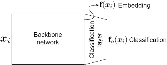
Various loss functions exist for supervised metric learning by neural networks. Supervised loss functions can teach the network to separate classes in the embedding space (Sikaroudi et al., 2020b). For this, we use a network whose last layer is for classification of data points. The features of the one-to-last layer can be used for feature embedding. The last layer after the embedding features is named the classification layer. The structure of this network is shown in Fig. 3. Let the -th point in the mini-batch be denoted by and its label be denoted by . Suppose the network has one output neuron and its output for the input is denoted by . This output is the estimated class label by the network. We denote output of the the one-to-last layer by where is the number of neurons in that layer which is equivalent to the dimensionality of the embedding space. The last layer of network, connecting the neurons to the output neuron is a fully-connected layer. The network until the one-to-last layer can be any feed-forward or convolutional network depending on the type of data. If the network is convolutional, it should be flattened at the one-to-last layer. The network learns to classify the classes, by the supervised loss functions, so the features of the one-to-last layers will be discriminating features and suitable for embedding.
5.2.1 Mean Squared Error and Mean Absolute Value Losses
One of the supervised losses is the Mean Squared Error (MSE) which makes the estimated labels close to the true labels using squared norm:
| (148) |
One problem with this loss function is exaggerating outliers because of the square but its advantage is its differentiability. Another loss function is the Mean Absolute Error (MAE) which makes the estimated labels close to the true labels using norm or the absolute value:
| (149) |
The distance used in this loss is also named the Manhattan distance. This loss function does not have the problem of MSE and it can be used for imposing sparsity in the embedding. It is not differentiable at the point but as the derivatives are calculated numerically by the neural network, this is not a big issue nowadays.
5.2.2 Huber and KL-Divergence Losss
Another loss function is the Huber loss which is a combination of the MSE and MAE to have the advantages of both of them:
| (150) | ||||
KL-divergence loss function makes the distribution of the estimated labels close to the distribution of the true labels:
| (151) |
5.2.3 Hinge Loss
If there are two classes, i.e. , we can have true labels as . In this case, a possible loss function is the Hinge loss:
| (152) |
where and is the margin. If the signs of the estimated and true labels are different, the loss is positive which should be minimized. If the signs are the same and , then the loss function is zero. If the signs are the same but , the loss is positive and should be minimized because the estimation is correct but not with enough margin from the incorrect estimation.
5.2.4 Cross-entropy Loss
For any number of classes, denoted by , we can have a cross-entropy loss. For this loss, we have neurons, rather than one neuron, at the last layer. In contrast to the MSE, MAE, Huber, and KL-divergence losses which use linear activation function at the last layer, cross-entropy requires softmax or sigmoid activation function at the last layer so the output values are between zero and one. For this loss, we have outputs, i.e. (continuous values between zero and one), and the true labels are one-hot encoded, i.e., . This loss is defined as:
| (153) |
where and denote the -th element of and , respectively. Minimizing this loss separates classes for classification; this separation of classes also gives us discriminating embedding in the one-to-last layer (Sikaroudi et al., 2020b; Boudiaf et al., 2020).
The reason for why cross-entropy can be suitable for metric learning is theoretically justified in (Boudiaf et al., 2020), explained in the following. Consider the mutual information between the true labels and the estimated labels :
| (154) | ||||
| (155) |
where denotes entropy. On the one hand, Eq. (154) has a generative view which exists in the metric learning loss functions generating embedding features. Eq. (155), one the other hand, has a discriminative view used in the cross-entropy loss function. Therefore, the metric learning losses and the cross-entropy loss are related. It is shown in (Boudiaf et al., 2020, Proposition 1) that the cross-entropy is an upper-bound on the metric learning losses so its minimization for classification also provides embedding features.
It is noteworthy that another supervised loss function is triplet loss, introduced in the next section. Triplet loss can be used for both hard labels (for classification) and soft labels (for similarity and dissimilarity of points). The triplet loss also does not need a last classification layer; therefore, the embedding layer can be the last layer for this loss.
5.3 Metric Learning by Siamese Networks
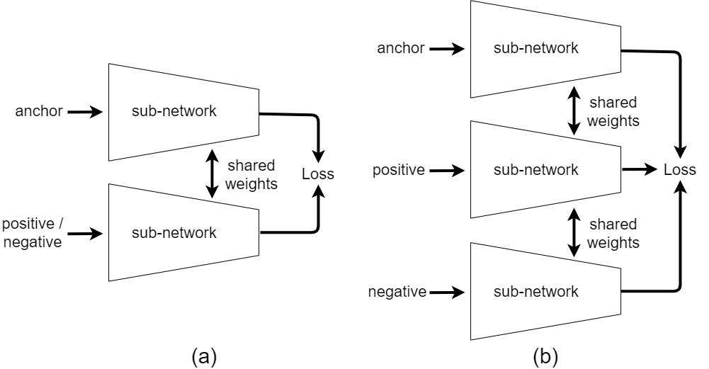
5.3.1 Siamese and Triplet Networks
One of the important deep metric learning methods is Siamese network which is widely used for feature extraction. Siamese network, originally proposed in (Bromley et al., 1993), is a network consisting of several equivalent sub-networks sharing their weights. The number of sub-networks in a Siamese network can be any number but it usually is two or three. A Siamese network with three sub-networks is also called a triplet network (Hoffer & Ailon, 2015). The weights of sub-networks in a Siamese network are trained in a way that the intra- and inter-class variances are decreased and increased, respectively. In other words, the similar points are pushed toward each other while the dissimilar points are pulled away from one another. Siamese networks have been used in various applications such as computer vision (Schroff et al., 2015) and natural language processing (Yang et al., 2020).
5.3.2 Pairs and Triplets of Data Points
Depending on the number of sub-networks in the Siamese network, we have loss functions for training. The loss functions of Siamese networks usually require pairs or triplets of data points. Siamese networks do not use the data points one by one but we need to make pairs or triplets of points out of dataset for training a Siamese network. For making the pairs or triplets, we consider every data point as the anchor point, denoted by . Then, we take one of the similar points to the anchor point as the positive (or neighbor) point, denoted by . We also take one of the dissimilar points to the anchor point as the negative (or distant) point, denoted by . If class labels are available, we can use them to find the positive point as one of the points in the same class as the anchor point, and to find the the negative point as one of the points in a different class from the anchor point’s class. Another approach is to augment the anchor point, using one of the augmentation methods, to obtain a positive points for the anchor point (Khodadadeh et al., 2019; Chen et al., 2020).
For Siamese networks with two sub-networks, we make pairs of anchor-positive points and anchor-negative points , where is the number of pairs. For Siamese networks with three sub-networks, we make triplets of anchor-positive-negative points , where is the number of triplets. If we consider every point of dataset as an anchor, the number of pairs/triplets is the same as the number of data points, i.e., .
Various loss functions of Siamese networks use pairs or triplets of data points to push the positive point towards the anchor point and pull the negative point away from it. Doing this iteratively for all pairs or triplets will make the intra-class variances smaller and the inter-class variances larger for better discrimination of classes or clusters. Later in the following, we introduce some of the loss functions for training a Siamese network.
5.3.3 Implementation of Siamese Networks
A Siamese network with two and three sub-networks is depicted in Fig. 4. We denote the output of Siamese network for input by where is the dimensionality of embedding (or the number of neurons at the last layer of the network) which is usually much less than the dimensionality of data, i.e., . Note that the sub-networks of a Siamese network can be any fully-connected or convolutional network depending on the type of data. The used network structure for the sub-networks is usually called the backbone network.

The weights of sub-networks are shared in the sense that the values of their weights are equal. Implementation of a Siamese network can be done in two ways:
-
1.
We can implement several sub-networks in the memory. In the training phase, we feed every data point in the pairs or triplets to one of the sub-networks and take the outputs of sub-networks to have , , and . We use these in the loss function and update the weights of only one of the sub-networks by backpropagation (Ghojogh et al., 2021c). Then, we copy the updated weights to the other sub-networks. We repeat this for all mini-batches and epochs until convergence. In the test phase, we feed the test point to only one of the sub-networks and get the output as its embedding.
-
2.
We can implement only one sub-network in the memory. In the training phase, we feed the data points in the pairs or triplets to the sub-network ont by one and take the outputs of sub-network to have , , and . We use these in the loss function and update the weights of the sub-network by backpropagation (Ghojogh et al., 2021c). We repeat this for all mini-batches and epochs until convergence. In the test phase, we feed the test point to the sub-network and get the output as its embedding.
The advantage of the first approach is to have all the sub-networks ready and we do not need to feed the points of pairs or triplets one by one. Its disadvantage is using more memory. As the number of points in the pairs or triplets is small (i.e., only two or three), the second approach is more recommended as it is memory-efficient.
5.3.4 Contrastive Loss
One loss function for Siamese networks is the contrastive loss which uses the anchor-positive and anchor-negative pairs of points. Suppose, in each mini-batch, we have pairs of points some of which are anchor-positive and some are anchor-negative pairs. The points in an anchor-positive pair are similar, i.e. , and the points in an anchor-negative pair are dissimilar, i.e. , where and denote the similar and dissimilar sets.
– Contrastive Loss: We define:
| (158) |
The main contrastive loss was proposed in (Hadsell et al., 2006) and is:
| (159) | ||||
where is the margin and is the standard Hinge loss. The first term of loss minimizes the embedding distances of similar points and the second term maximizes the embedding distances of dissimilar points. As shown in Fig. 5-b, it tries to make the distances of similar points as small as possible and the distances of dissimilar points at least greater than a margin (because the term inside the Hinge loss should become close to zero).
– Generalized Contrastive Loss: The , defined in Eq. (158), is used in the contrastive loss, i.e., Eq. (159). This variable is binary and a hard measure of similarity and dissimilarity. Rather than this hard measure, we can have a soft measure of similarity and dissimilarity, denoted by , which states how similar and are. This measure is between zero (completely similar) and one (completely dissimilar). It can be either given by the dataset as a hand-set measure or can be computed using any similarity measure such as the cosine function:
| (160) |
In this case, the pairs need not be completely similar or dissimilar points but they can be any two random points from the dataset with some level of similarity/dissimilarity. The generalized contrastive loss generalizes the contrastive loss using this soft measure of similarity (Leyva-Vallina et al., 2021):
| (161) | ||||
5.3.5 Triplet Loss
One of the losses for Siamese networks with three sub-networks is the triplet loss (Schroff et al., 2015) which uses the triplets in mini-batches, denoted by . It is defined as:
| (162) |
where is the margin and is the standard Hinge loss. As shown in Fig. 5-c, because of the used Hinge loss, this loss makes the distances of dissimilar points greater than the distances of similar points by at least a margin ; in other words, there will be a distance of at least margin between the positive and negative points. This loss desires to eventually have:
| (163) |
for all triplets. The triplet loss is closely related to the cost function for spectral large margin metric learning (Weinberger et al., 2006; Weinberger & Saul, 2009) (see Section 3.2.1). It is also noteworthy that using the triplet loss as regularization for cross-entropy loss has been shown to increase robustness of network to some adversarial attacks (Mao et al., 2019).
5.3.6 Tuplet Loss
In triplet loss, i.e. Eq. (162), we use one positive and one negative point per anchor point. The tuplet loss (Sohn, 2016) uses several negative points per anchor point. If denotes the number of negative points per anchor point and denotes the -th negative point for , the tuplet loss is (Sohn, 2016):
| (164) | ||||
This loss function pushes multiple negative points away from the anchor point simultaneously.
5.3.7 Neighborhood Component Analysis Loss
Neighborhood Component Analysis (NCA) (Goldberger et al., 2005) was originally proposed as a spectral metric learning method (see Section 4.2.1). After the success of deep learning, it was used as the loss function of Siamese networks where we minimize the negative log-likelihood using Gaussian distribution or the softmax form within the mini-batch. Assume we have classes in every mini-batch. We denote the class index of by and the data points of the -th class in the mini-batch by . The NCA loss is:
| (165) | ||||
The numerator minimizes the distances of similar points and the denominator maximizes the distances of dissimilar points.
5.3.8 Proxy Neighborhood Component Analysis Loss
Computation of terms, especially the normalization factor in the denominator, is time- and memory-consuming in the NCA loss function (see Eq. (165)). Proxy-NCA loss functions define some proxy points in the embedding space of network and use them in the NCA loss to accelerate computation and make it memory-efficient (Movshovitz-Attias et al., 2017). The proxies are representatives of classes in the embedding space and they can be defined in various ways. The simplest way is to define the proxy of every class as the mean of embedded points of that class. Of course, new mini-batches come during training. We can accumulate the embedded points of mini-batches and update the proxies after training the network by every mini-batch. Another approach for defining proxies is to cluster the embedded points into clusters (e.g., by K-means) and use the centroid of clusters.
Let the set of proxies be denotes by whose cardinality is the number of classes, i.e., . Every embedded point is assigned to one of the proxies by (Movshovitz-Attias et al., 2017):
| (166) |
or we can assign every point to the proxy of its own class. Let denote the proxy associated with the -th class. The Proxy-NCA loss is the NCA loss, i.e. Eq. (165), but using proxies (Movshovitz-Attias et al., 2017):
| (167) | ||||
It is shown in (Movshovitz-Attias et al., 2017) that the Proxy-NCA loss, i.e. Eq. (167), is an upper-bound on the NCA loss, i.e. Eq. (165); hence, its minimization also achieves the goal of NCA. Comparing Eqs. (165) and (167) shows that Proxy-NCA is faster and more efficient than NCA because it uses only proxies of negative classes rather than using all negative points in the mini-batch. Proxy-NCA has also been used in feature extraction from medical images (Teh & Taylor, 2020). It is noteworthy that we can incorporate temperature scaling (Hinton et al., 2014) in the Proxy-NCA loss. The obtained loss is named Proxy-NCA++ (Teh et al., 2020) and is defined as:
| (168) | ||||
where is the temperature which is a hyper-parameter.
5.3.9 Softmax Triplet Loss
Consider a mini-batch containing points from classes where is the class index of and denotes the points of the -th class in the mini-batch. We can use the softmax function or the Gaussian distribution for the probability that the point takes as its neighbor. Similar to Eq. (84) or Eq. (165), we can have the softmax function used in NCA (Goldberger et al., 2005):
| (169) |
Another approach for the softmax form is to use inner product in the exponent (Ye et al., 2019):
| (170) |
The loss function for training the network can be the negative log-likelihood which can be called the softmax triplet loss (Ye et al., 2019):
| (171) | ||||
This decreases and increases the distances of similar points and dissimilar points, respectively.
5.3.10 Triplet Global Loss
The triplet global loss (Kumar BG et al., 2016) uses the mean and variance of the anchor-positive pairs and anchor-negative pairs. It is defined as:
| (172) |
where is the regularization parameter, is the margin, the means of pairs are:
and the variances of pairs are:
The first term of this loss minimizes the variances of anchor-positive and anchor-negative pairs. The second term, however, discriminates the anchor-positive pairs from the anchor-negative pairs. Hence, the negative points are separated from the positive points.
5.3.11 Angular Loss
For a triplet , consider a triangle whose vertices are the anchor, positive, and negative points. To satisfy Eq. (163) in the triplet loss, the angle at the vertex should be small so the edge becomes larger than the edge . Hence, we need to have and upper bound on the angle at the vertex . If , the angular loss is defined to be (Wang et al., 2017):
| (173) | ||||
This loss reduces the distance of the anchor and positive points and increases the distance of anchor and and the upper bound . This increases the distance of the anchor and negative points for discrimination of dissimilar points.
5.3.12 SoftTriple Loss
If we normalize the points to have unit length, Eq. (163) can be restated by using inner products:
| (174) |
whose margin is not exactly equal to the margin in Eq. (163). Consider a Siamese network whose last layer’s weights are where is the dimensionality of the one-to-last layer and is the number of classes and the number of output neurons. We consider centers for the embedding of every class; hence, we define as for its -th center. It is shown in (Qian et al., 2019) that softmax loss results in Eq. (174). Therefore, we can use the SoftTriple loss for training a Siamese network (Qian et al., 2019):
| (175) | ||||
where are hyper-parameters, is the label of , and:
This loss increases and decreases the intra-class and inter-class distances, respectively.
5.3.13 Fisher Siamese Losses
Fisher Discriminant Analysis (FDA) (Fisher, 1936; Ghojogh et al., 2019b) decreases the intra-class variance and increases the inter-class variance by maximizing the Fisher criterion. This idea is very similar to the idea of loss functions for Siamese networks. Hence, we can combine the methods of FDA and Siamese loss functions.
Consider a Siamese network whose last layer is denoted by the projection matrix . We consider the features of the one-to-last layer in the mini-batch. The covariance matrices of similar points and dissimilar points (one-to-last layer features) in the mini-batch are denoted by and . These covariances become and , respectively, after the later layer’s projection because of the quadratic characteristic of covariance. As in FDA, we can maximize the Fisher criterion or equivalently minimize the negative Fisher criterion:
This problem is ill-posed because it increases the total covariance of embedded data to increase the term . Hence, we add minimization of the total covariance as the regularization term:
where is the regularization parameter and is the covariance of all points of the mini-batch in the one-to-last layer. The total scatter can be written as the summation of and ; hence:
where . Inspired by Eq. (162), we can have the following loss, named the Fisher discriminant triplet loss (Ghojogh et al., 2020f):
| (176) | ||||
where is the margin. Backpropagating the error of this loss can update both and other layers of network. Note that the summation over the mini-batch is integrated in the computation of covariance matrices and . Inspired by Eq. (159), we can also have the Fisher discriminant contrastive loss (Ghojogh et al., 2020f):
| (177) | ||||
Note that the variable used in the contrastive loss (see Eq. (158)) is already used in computation of the covariances and . There exist some other loss functions inspired by Fisher discriminant analysis but they are not used for Siamese networks. Those methods will be introduced in Section 5.4.
5.3.14 Deep Adversarial Metric Learning
In deep adversarial metric learning (Duan et al., 2018), negative points are generated in an adversarial learning (Goodfellow et al., 2014; Ghojogh et al., 2021b). In this method, we have a generator which tries to generate negative points fooling the metric learning. Using triplet inputs , the loss function of generator is (Duan et al., 2018):
| (178) | ||||
where are the regularization parameters. This loss makes the generated negative point close to the real negative point (to be negative) and the anchor point (for fooling metric learning adversarially). The Hinge loss makes the generated negative point different from the anchor and positive points so it also acts like a real negative. If denotes any loss function for Siamese network, such as the triplet loss, the total loss function in deep adversarial metric learning is minimizing where is the regularization parameter (Duan et al., 2018). It is noteworthy that there exists another adversarial metric learning which is not for Siamese networks but for cross-modal data (Xu et al., 2019a).
5.3.15 Triplet Mining
In every mini-batch containing data points from classes, we can select and use triplets of data points in different ways. For example, we can use all similar and dissimilar points for every anchor point as positive and negative points, respectively. Another approach is to only use some of the similar and dissimilar points within the mini-batch. These approaches for selecting and using triplets are called triplet mining (Sikaroudi et al., 2020a). In the following, we review some of the most important triplet mining methods. We use triplet mining methods for the triplet loss, i.e., Eq. (162). Suppose is the mini-batch size, is the class index of , denotes the points of the -th class in the mini-batch, and denotes the data points in the mini-batch.
– Batch-all: Batch-all triplet mining (Ding et al., 2015) considers every point in the mini-batch as an anchor point. All points in the mini-batch which are in the same class the anchor point are used as positive points. All points in the mini-batch which are in a different class from the class of anchor point are used as negative points:
| (179) | ||||
Batch-all mining makes use of all data points in the mini-batch to utilize all available information.
– Batch-hard: Batch-hard triplet mining (Hermans et al., 2017) considers every point in the mini-batch as an anchor point. The hardest positive, which is the farthest point from the anchor point in the same class, is used as the positive point. The hardest negative, which is the closest point to the anchor point from another class, is used as the negative point:
| (180) | ||||
Bath-hard mining uses hardest points so that the network learns the hardest cases. By learning the hardest cases, other cases are expected to be learned properly. Learning the hardest cases can also be justified by the opposition-based learning (Tizhoosh, 2005). Batch-hard mining has been used in many applications such as person re-identification (Wang et al., 2019).
– Batch-semi-hard: Batch-semi-hard triplet mining (Schroff et al., 2015) considers every point in the mini-batch as an anchor point. All points in the mini-batch which are in the same class the anchor point are used as positive points. The hardest negative (closest to the anchor point from another class), which is farther than the positive point, is used as the negative point:
| (181) | ||||
– Easy-positive: Easy-positive triplet mining (Xuan et al., 2020) considers every point in the mini-batch as an anchor point. The easiest positive (closest to the anchor point from the same class) is used as the positive point. All points in the mini-batch which are in a different class from the class of anchor point are used as negative points:
| (182) | ||||
We can use this triplet mining approach in NCA loss function such as in Eq. (170). For example, we can have (Xuan et al., 2020):
| (183) | ||||
where the embeddings for all points of the mini-batch are normalized to have length one.
– Lifted embedding loss: The lifted embedding loss (Oh Song et al., 2016) is related to the anchor-positive distance and the smallest (hardest) anchor-negative distance:
| (184) | ||||
This loss is using triplet mining because of using extreme distances. Alternatively, another version of this loss function uses logarithm and exponential operators (Oh Song et al., 2016):
| (185) | ||||
– Hard mining center-triplet loss: Let the mini-batch contain data points from classes. Hard mining center–triplet loss (Lv et al., 2019) considers the mean of every class as an anchor point. The hardest (farthest) positive point and the hardest (closest) negative point are used in this loss as (Lv et al., 2019):
| (186) | ||||
where denotes the mean of the -th class.
– Triplet loss with cross-batch memory: A version of triplet loss can be (Wang et al., 2020a):
| (187) | ||||
This triplet loss can use a cross-batch memory where we accumulate a few latest mini-batches. Every coming mini-batch updates the memory. Let the capacity of the memory be points and the mini-batch size be . Let denote the -th data point in the memory. The triplet loss with cross-batch memory is defined as (Wang et al., 2020a):
| (188) | ||||
which takes the positive and negative points from the memory rather than from the coming mini-batch.
5.3.16 Triplet Sampling
Rather than using the extreme (hardest or easiest) positive and negative points (Sikaroudi et al., 2020a), we can sample positive and negative points from the points in the mini-batch or from some distributions. There are several approaches for the positive and negative points to be sampled (Ghojogh, 2021):
-
•
Sampled by extreme distances of points,
-
•
Sampled randomly from classes,
-
•
Sampled by distribution but from existing points,
-
•
Sampled stochastically from distributions of classes.
These approaches are used for triplet sampling. The first approach was introduced in Section 5.3.15. The first, second, and third approaches sample the positive and negative points from the set of points in the mini-batch. This type of sampling is called survey sampling (Ghojogh et al., 2020e). The third and fourth approaches sample points from distributions stochastically. In the following, we introduce some of the triplet sampling methods.
– Distance weighted sampling: Distance weighted sampling (Wu et al., 2017) is a method in the third approach, i.e., sampling by distribution but from existing points. The distribution of the pairwise distances is proportional to (Wu et al., 2017):
where is the number of points in the mini-batch and is the dimensionality of embedding space (i.e., the number of neurons in the last layer of the Siamese network). In every mini-batch, we consider every point once as an anchor point. For an anchor point, we consider all points of the mini-batch which are in a different class as candidates for the negative point. We sample a negative point, denoted by from these candidates (Wu et al., 2017):
where is a hyperparameter to ensure that all candidates have a chance to be chosen. This sampling is performed for every mini-batch. The loss function in distance weighted sampling is (Wu et al., 2017):
| (189) | ||||
– Sampling by Bayesian updating theorem: We can sample triplets from distributions of classes which is the forth approach of sampling, mentioned above. One method for this sampling is using the Bayesian updating theorem (Sikaroudi et al., 2021) which is updating the posterior by the Bayes’ rule from some new data. In this method, we assume -dimensional Gaussian distribution for every class in the embedding space where is the dimensionality of embedding space. We accumulate the embedded points for every class when the new mini-batches are introduced to the network. The distributions of classes are updated based on both the existing points available so far and the new-coming data points. It can be shown that the posterior of mean and covariance of a Gaussian distribution is a normal inverse Wishart distribution (Murphy, 2007). The mean and covariance of a Gaussian distribution have a generalized Student-t distribution and inverse Wishart distribution, respectively (Murphy, 2007). Let the so-far available data have sample size , mean , and covariance . Also, let the newly coming data have sample size , mean , and covariance . We update the mean and covariance by expectation of these distributions (Sikaroudi et al., 2021):
where:
The updated mean and covariance are used for Gaussian distributions of the classes. Then, we sample triplets from the distributions of classes rather than from the points of mini-batch. We consider every point of the new mini-batch as an anchor point and sample a positive point from the distribution of the same class. We sample negative points from the distributions of other classes. If this triplet sampling procedure is used with triplet and contrastive loss functions, the approach is named Bayesian Updating with Triplet loss (BUT) and Bayesian Updating with NCA loss (BUNCA) (Sikaroudi et al., 2021).
– Hard negative sampling: Let the anchor, positive, and negative points be denoted by , , and , respectively. Consider the following distributions for the negative and positive points (Robinson et al., 2021):
where is a hyper-parameter. The loss function with hard negative sampling is (Robinson et al., 2021):
| (190) | ||||
where positive and negative points are sampled from positive and negative distributions defined above. The expectations can be estimated using the Monte Carlo approximation (Ghojogh et al., 2020e). This time of triplet sampling is a method in the fourth type of triplet sampling, i.e., sampling stochastically from distributions of classes.
5.4 Deep Discriminant Analysis Metric Learning
Deep discriminant analysis metric learning methods use the idea of Fisher discriminant analysis (Fisher, 1936; Ghojogh et al., 2019b) in deep learning, for learning an embedding space which separates classes. Some of these methods are deep probabilistic discriminant analysis (Li et al., 2019), discriminant analysis with virtual samples (Kim & Song, 2021), Fisher Siamese losses (Ghojogh et al., 2020f), and deep Fisher discriminant analysis (Díaz-Vico et al., 2017; Díaz-Vico & Dorronsoro, 2019). The Fisher Siamese losses were already introduced in Section 5.3.13.
5.4.1 Deep Probabilistic Discriminant Analysis
Deep probabilistic discriminant analysis (Li et al., 2019) minimizes the inverse Fisher criterion:
| (191) | ||||
where is the mini-batch size, is the number of classes, is the class label of , denotes covariance, denotes variance, is the prior of the -th class (estimated by the ratio of class population to the total number of points in the mini-batch), is because of the law of total variance, and is because of the definition of expectation. The numerator and denominator represent the intra-class and inter-class variances, respectively.
5.4.2 Discriminant Analysis with Virtual Samples
In discriminant analysis metric learning with virtual samples (Kim & Song, 2021), we consider any backbone network until the one-to-last layer of neural network and a last layer with linear activation function. Let the outputs of the one-to-last layer be denoted by and the weights of the last layer be . We compute the intra-class scatter and inter-class scatter for the one-to-last layer’s features . If we see the last layer as a Fisher discriminant analysis model with projection matrix , the solution is the eigenvalue problem (Ghojogh et al., 2019a) for . Let denote the -th eigenvalue of this problem.
Assume and denote the similar and dissimilar points in the mini-batch where . We define (Kim & Song, 2021):
where is the -th element of . We sample numbers, namely virtual samples, from the uniform distribution where is a small positive number and is the mean of eigenvalues ’s. The virtual samples are put in a vector .
The loss function for discriminant analysis with virtual samples is (Kim & Song, 2021):
| (192) | ||||
where is the norm, , is the margin, and the second term is maximization of the Fisher criterion.
5.4.3 Deep Fisher Discriminant Analysis
It is shown in (Hart et al., 2000) that the solution to the following least squares problem is equivalent to the solution of Fisher discriminant analysis:
| (193) |
where is the Frobenius norm, is the row-wise stack of data points, where is the centering matrix, is the one-hot-encoded labels stacked row-wise, is the diagonal matrix whose -th element is the cardinality of the -th class.
Deep Fisher discriminant analysis (Díaz-Vico et al., 2017; Díaz-Vico & Dorronsoro, 2019) implements Eq. (193) by a nonlinear neural network with loss function:
| (194) |
where is the weights of network, denotes the row-wise stack of points in the mini-batch of size , is computed in every mini-batch, and is the row-wise stack of output embeddings of the network. After training, the output is the embedding for the input point .
5.5 Multi-Modal Deep Metric Learning
Data has several modals where a separate set of features is available for every modality of data. In other words, we can have several features for every data point. Note that the dimensionality of features may differ. Multi-modal deep metric learning (Roostaiyan et al., 2017) addresses this problem in metric learning. Let denote the number of modalities. Consider stacked autoencoders each of which is for one of the modalities. The -th autoencoder gets the -th modality of the -th data point, denoted by , and reconstructs it as output, denoted by . The embedding layer, or the layer between encoder and decoder, is shared between all autoencoders. We denote the output of this shared embedding layer by . The loss function for training the stacked autoencoders with the shared embedding layer can be (Roostaiyan et al., 2017):
| (195) | ||||
where are the regularization parameters and are the margins. The first term is the reconstruction loss and the second and third terms are for metric learning which collapses each class to a margin and discriminates classes by a margin . This loss function is optimized in a stacked autoencoder setup (Hinton & Salakhutdinov, 2006; Wang et al., 2014). Then, it is fine-tuned by backpropagation (Ghojogh et al., 2021f). After training, the embedding layer can be used for embedding data points. Note that another there exists another multi-modal deep metric learning, which is (Xu et al., 2019a).
5.6 Geometric Metric Learning by Neural Network
There exist some works, such as (Huang & Van Gool, 2017), (Hauser, 2017), and (Hajiabadi et al., 2019), which have implemented neural networks on the Riemannian manifolds. Layered geometric learning (Hajiabadi et al., 2019) implements Geometric Mean Metric Learning (GMML) (Zadeh et al., 2016) (recall Section 3.7.1) in a neural network framework. In this method, every layer of network is a metric layer which projects the output of its previous layer onto the subspace of its own metric (see Proposition 2 and Proposition 8).
For the -th layer of network, we denote the weight matrix (i.e., the projection matrix of metric) and the output of layer for the -th data point by and , respectively. Hence, the metric in the -th layer models . Consider the dataset of points . We denote the output of the -th layer by . The projection of a layer onto its metric subspace is .
Every layer solves the optimization problem of GMML (Zadeh et al., 2016), i.e., Eq. (61). For this, we start from the first layer and proceed to the last layer by feed-propagation. The -th layer computes and for by Eq. (14). Then, the solution of optimization (61) is computed which is the Eq. (65), i.e., . Then, using Eq. (9), we decompose the obtained to find . Then, data points are projected onto the metric subspace as .
If we want the output of layers lie on the positive semi-definite manifold, the activation function of every layer can be projection onto the positive semi-definite cone (Ghojogh et al., 2021c):
where and are the eigenvectors and eigenvalues of , respectively. This activation function is called the eigenvalue rectification layer in (Huang & Van Gool, 2017). Finally, it is noteworthy that there is another work, named backprojection (Ghojogh et al., 2020d), which has similar idea but in the Euclidean and Hilbert spaces and not in the Riemannian space.
5.7 Few-shot Metric Learning
Few-shot learning refers to learning from a few data points rather than from a large enough dataset. Few-shot learning is used for domain generalization to be able to use for unseen data in the test phase (Wang et al., 2020b). The training phase of few-shot learning is episodic where in every iteration or so-called episode of training, we have a support set and a query set. In other words, the training dataset is divided into mini-batches where every mini-batch contains a support set and a query set (Triantafillou et al., 2020). Consider a training dataset with classes and a test dataset with classes. As mentioned before, test and training datasets are usually disjoint in few-shot learning so it is useful for domain generalization. In every episode, also called the task or the mini-batch, we train using some (and not all) training classes by randomly sampling from classes.
The support set is where and denote the data point and its label, respectively. The query set is . The training data of every episode (mini-batch) is the union of the support and query sets. At every episode, we randomly sample classes out of the total classes of training dataset, where we usually have . Then, we sample training data points from these selected classes. These form the support set. This few-shot setup is called -way, -shot in which the support set contains classes and points in every class. The number of classes and every class’s points in the query set of every episode may or may not be the same as in the support set.
In every episode of the training phase of few-shot learning, we update the network weights by back-propagating error using the support set. These updated weights are not finalized yet. We feed the query set to the network with the updated weights and back-propagate error using the query set. This second back-propagation with the query set updates the weights of network finally at the end of episode. In other words, the query set is used to evaluate how good the update by support set are. This learning procedure for few-shot learning is called meta-learning (Finn et al., 2017).
There are several family of methods for few-shot learning, one of which is some deep metric learning methods. Various metric learning methods have been proposed for learning from few-shot data. For example, Siamese network, introduced in Section 5.3, has been used for few-shot learning (Koch et al., 2015; Li et al., 2020). In the following, we introduce two metric learning methods for few-shot learning.
5.7.1 Multi-scale Metric Learning
Multi-scale metric learning (Jiang et al., 2020) learns the embedding space by learning multiple scales of middle features in the training process. It has several steps. In the first step, we use a pre-trained network with multiple output layers which produce several different scales of features for both the support and query sets. In the second step, within every scale of support set, we take average of the features in every class. This gives us features for every scale in the support set. This and the features of the query set are fed to the third step. In the third step, we feed every scale to a sub-network where larger scales are fed to sub-networks with more number of layers as they contain more information to process. These sub-networks are concatenated to give a scalar output for every data point with multiple scales of features. Hence, we obtain a scalar score for every data point in the support and query sets. Finally, a combination of a classification loss function, such as the cross-entropy loss (see Eq. (153)), and triplet loss (see Eq. 162) is used in the support-query setup explained before.
5.7.2 Metric Learning with Continuous Similarity Scores
Another few-shot metric learning is (Xu et al., 2019b) which takes pairs of data points as the input support and query sets. For the pair , consider binary similarity score, , defined as:
| (198) |
where and denote the sets of similar and dissimilar points, respectively. We can define continuous similarity score, , as (Xu et al., 2019b):
| (201) |
where and is the normalized squared Euclidean distance (we normalize distances within every mini-batch). The ranges of these continuous similarities are:
In every episode (mini-batch), the pairs are fed to a network with several feature vector outputs. For every pair , these feature vectors are fed to another network which outputs a scalar similarity score . The loss function of metric learning in this method is (Xu et al., 2019b):
| (202) | ||||||
| subject to | ||||||
where is the regularization parameter and is the mini-batch of the support or query set depending on whether it is the phase of support or query.
6 Conclusion
This was a tutorial and survey on spectral, probabilistic, and deep metric learning. We started with defining distance metric. In spectral methods, we covered methods using scatters of data, methods using Hinge loss, locally linear metric adaptation, kernel methods, geometric methods, and adversarial metric learning. In probabilistic category, we covered collapsing classes, neighborhood component analysis, Bayesian metric learning, information theoretic methods, and empirical risk minimization approaches. In deep learning methods, we explain reconstruction autoencoders, supervised loss functions, Siamese networks, deep discriminant analysis methods, multi-modal learning, geometric deep metric learning, and few-shot metric learning.
References
- Absil et al. (2009) Absil, P-A, Mahony, Robert, and Sepulchre, Rodolphe. Optimization algorithms on matrix manifolds. Princeton University Press, 2009.
- Alipanahi et al. (2008) Alipanahi, Babak, Biggs, Michael, and Ghodsi, Ali. Distance metric learning vs. Fisher discriminant analysis. In Proceedings of the 23rd national conference on Artificial intelligence, volume 2, pp. 598–603, 2008.
- Arsigny et al. (2007) Arsigny, Vincent, Fillard, Pierre, Pennec, Xavier, and Ayache, Nicholas. Geometric means in a novel vector space structure on symmetric positive-definite matrices. SIAM journal on matrix analysis and applications, 29(1):328–347, 2007.
- Baghshah & Shouraki (2009) Baghshah, Mahdieh Soleymani and Shouraki, Saeed Bagheri. Semi-supervised metric learning using pairwise constraints. In Twenty-First International Joint Conference on Artificial Intelligence, 2009.
- Baghshah & Shouraki (2010) Baghshah, Mahdieh Soleymani and Shouraki, Saeed Bagheri. Kernel-based metric learning for semi-supervised clustering. Neurocomputing, 73(7-9):1352–1361, 2010.
- Bar-Hillel et al. (2003) Bar-Hillel, Aharon, Hertz, Tomer, Shental, Noam, and Weinshall, Daphna. Learning distance functions using equivalence relations. In Proceedings of the 20th international conference on machine learning (ICML-03), pp. 11–18, 2003.
- Bar-Hillel et al. (2005) Bar-Hillel, Aharon, Hertz, Tomer, Shental, Noam, Weinshall, Daphna, and Ridgeway, Greg. Learning a mahalanobis metric from equivalence constraints. Journal of machine learning research, 6(6), 2005.
- Belkin & Niyogi (2001) Belkin, Mikhail and Niyogi, Partha. Laplacian eigenmaps and spectral techniques for embedding and clustering. In Advances in neural information processing systems, volume 14, pp. 585–591, 2001.
- Belkin & Niyogi (2002) Belkin, Mikhail and Niyogi, Partha. Laplacian eigenmaps and spectral techniques for embedding and clustering. In Advances in neural information processing systems, pp. 585–591, 2002.
- Bellet et al. (2013) Bellet, Aurélien, Habrard, Amaury, and Sebban, Marc. A survey on metric learning for feature vectors and structured data. arXiv preprint arXiv:1306.6709, 2013.
- Bellet et al. (2015) Bellet, Aurélien, Habrard, Amaury, and Sebban, Marc. Metric learning. Synthesis Lectures on Artificial Intelligence and Machine Learning, 9(1):1–151, 2015.
- Bhatia (2007) Bhatia, Rajendra. Positive definite matrices. Princeton university press, 2007.
- Bhutani et al. (2018) Bhutani, Mukul, Jawanpuria, Pratik, Kasai, Hiroyuki, and Mishra, Bamdev. Low-rank geometric mean metric learning. arXiv preprint arXiv:1806.05454, 2018.
- Boudiaf et al. (2020) Boudiaf, Malik, Rony, Jérôme, Ziko, Imtiaz Masud, Granger, Eric, Pedersoli, Marco, Piantanida, Pablo, and Ayed, Ismail Ben. A unifying mutual information view of metric learning: cross-entropy vs. pairwise losses. In European Conference on Computer Vision, pp. 548–564. Springer, 2020.
- Bromley et al. (1993) Bromley, Jane, Bentz, James W, Bottou, Léon, Guyon, Isabelle, LeCun, Yann, Moore, Cliff, Säckinger, Eduard, and Shah, Roopak. Signature verification using a “Siamese” time delay neural network. International Journal of Pattern Recognition and Artificial Intelligence, 7(04):669–688, 1993.
- Chang & Yeung (2004) Chang, Hong and Yeung, Dit-Yan. Locally linear metric adaptation for semi-supervised clustering. In Proceedings of the twenty-first international conference on Machine learning, pp. 20, 2004.
- Chen et al. (2018) Chen, Shuo, Gong, Chen, Yang, Jian, Li, Xiang, Wei, Yang, and Li, Jun. Adversarial metric learning. arXiv preprint arXiv:1802.03170, 2018.
- Chen et al. (2019) Chen, Shuo, Luo, Lei, Yang, Jian, Gong, Chen, Li, Jun, and Huang, Heng. Curvilinear distance metric learning. Advances in Neural Information Processing Systems, 32, 2019.
- Chen et al. (2020) Chen, Ting, Kornblith, Simon, Norouzi, Mohammad, and Hinton, Geoffrey. A simple framework for contrastive learning of visual representations. In International conference on machine learning, pp. 1597–1607, 2020.
- Cour et al. (2011) Cour, Timothee, Sapp, Ben, and Taskar, Ben. Learning from partial labels. The Journal of Machine Learning Research, 12:1501–1536, 2011.
- Cox & Cox (2008) Cox, Michael AA and Cox, Trevor F. Multidimensional scaling. In Handbook of data visualization, pp. 315–347. Springer, 2008.
- Davis et al. (2007) Davis, Jason V, Kulis, Brian, Jain, Prateek, Sra, Suvrit, and Dhillon, Inderjit S. Information-theoretic metric learning. In Proceedings of the 24th international conference on Machine learning, pp. 209–216, 2007.
- De Maesschalck et al. (2000) De Maesschalck, Roy, Jouan-Rimbaud, Delphine, and Massart, Désiré L. The mahalanobis distance. Chemometrics and intelligent laboratory systems, 50(1):1–18, 2000.
- De Vazelhes et al. (2020) De Vazelhes, William, Carey, CJ, Tang, Yuan, Vauquier, Nathalie, and Bellet, Aurélien. metric-learn: Metric learning algorithms in Python. Journal of Machine Learning Research, 21:138–1, 2020.
- Dhillon (2007) Dhillon, JVDI. Differential entropic clustering of multivariate Gaussians. Advances in Neural Information Processing Systems, 19:337, 2007.
- Díaz-Vico & Dorronsoro (2019) Díaz-Vico, David and Dorronsoro, José R. Deep least squares Fisher discriminant analysis. IEEE transactions on neural networks and learning systems, 31(8):2752–2763, 2019.
- Díaz-Vico et al. (2017) Díaz-Vico, David, Omari, Adil, Torres-Barrán, Alberto, and Dorronsoro, José Ramón. Deep Fisher discriminant analysis. In International Work-Conference on Artificial Neural Networks, pp. 501–512. Springer, 2017.
- Ding et al. (2015) Ding, Shengyong, Lin, Liang, Wang, Guangrun, and Chao, Hongyang. Deep feature learning with relative distance comparison for person re-identification. Pattern Recognition, 48(10):2993–3003, 2015.
- Dong (2019) Dong, Minghzi. Metric learning with Lipschitz continuous functions. PhD thesis, UCL (University College London), 2019.
- Duan et al. (2018) Duan, Yueqi, Zheng, Wenzhao, Lin, Xudong, Lu, Jiwen, and Zhou, Jie. Deep adversarial metric learning. In Proceedings of the IEEE Conference on Computer Vision and Pattern Recognition, pp. 2780–2789, 2018.
- Feng et al. (2018) Feng, Lin, Wang, Huibing, Jin, Bo, Li, Haohao, Xue, Mingliang, and Wang, Le. Learning a distance metric by balancing KL-divergence for imbalanced datasets. IEEE Transactions on Systems, Man, and Cybernetics: Systems, 49(12):2384–2395, 2018.
- Finn et al. (2017) Finn, Chelsea, Abbeel, Pieter, and Levine, Sergey. Model-agnostic meta-learning for fast adaptation of deep networks. In International Conference on Machine Learning, pp. 1126–1135, 2017.
- Fisher (1936) Fisher, Ronald A. The use of multiple measurements in taxonomic problems. Annals of eugenics, 7(2):179–188, 1936.
- Gautheron et al. (2019) Gautheron, Léo, Habrard, Amaury, Morvant, Emilie, and Sebban, Marc. Metric learning from imbalanced data. In 2019 IEEE 31st International Conference on Tools with Artificial Intelligence (ICTAI), pp. 923–930. IEEE, 2019.
- Ghodsi et al. (2007) Ghodsi, Ali, Wilkinson, Dana F, and Southey, Finnegan. Improving embeddings by flexible exploitation of side information. In IJCAI, pp. 810–816, 2007.
- Ghojogh (2021) Ghojogh, Benyamin. Data Reduction Algorithms in Machine Learning and Data Science. PhD thesis, University of Waterloo, 2021.
- Ghojogh & Crowley (2019) Ghojogh, Benyamin and Crowley, Mark. Unsupervised and supervised principal component analysis: Tutorial. arXiv preprint arXiv:1906.03148, 2019.
- Ghojogh et al. (2019a) Ghojogh, Benyamin, Karray, Fakhri, and Crowley, Mark. Eigenvalue and generalized eigenvalue problems: Tutorial. arXiv preprint arXiv:1903.11240, 2019a.
- Ghojogh et al. (2019b) Ghojogh, Benyamin, Karray, Fakhri, and Crowley, Mark. Fisher and kernel Fisher discriminant analysis: Tutorial. arXiv preprint arXiv:1906.09436, 2019b.
- Ghojogh et al. (2020a) Ghojogh, Benyamin, Ghodsi, Ali, Karray, Fakhri, and Crowley, Mark. Locally linear embedding and its variants: Tutorial and survey. arXiv preprint arXiv:2011.10925, 2020a.
- Ghojogh et al. (2020b) Ghojogh, Benyamin, Ghodsi, Ali, Karray, Fakhri, and Crowley, Mark. Multidimensional scaling, Sammon mapping, and Isomap: Tutorial and survey. arXiv preprint arXiv:2009.08136, 2020b.
- Ghojogh et al. (2020c) Ghojogh, Benyamin, Ghodsi, Ali, Karray, Fakhri, and Crowley, Mark. Stochastic neighbor embedding with Gaussian and Student-t distributions: Tutorial and survey. arXiv preprint arXiv:2009.10301, 2020c.
- Ghojogh et al. (2020d) Ghojogh, Benyamin, Karray, Fakhri, and Crowley, Mark. Backprojection for training feedforward neural networks in the input and feature spaces. In International Conference on Image Analysis and Recognition, pp. 16–24. Springer, 2020d.
- Ghojogh et al. (2020e) Ghojogh, Benyamin, Nekoei, Hadi, Ghojogh, Aydin, Karray, Fakhri, and Crowley, Mark. Sampling algorithms, from survey sampling to Monte Carlo methods: Tutorial and literature review. arXiv preprint arXiv:2011.00901, 2020e.
- Ghojogh et al. (2020f) Ghojogh, Benyamin, Sikaroudi, Milad, Shafiei, Sobhan, Tizhoosh, Hamid R, Karray, Fakhri, and Crowley, Mark. Fisher discriminant triplet and contrastive losses for training Siamese networks. In 2020 international joint conference on neural networks (IJCNN), pp. 1–7. IEEE, 2020f.
- Ghojogh et al. (2021a) Ghojogh, Benyamin, Ghodsi, Ali, Karray, Fakhri, and Crowley, Mark. Factor analysis, probabilistic principal component analysis, variational inference, and variational autoencoder: Tutorial and survey. arXiv preprint arXiv:2101.00734, 2021a.
- Ghojogh et al. (2021b) Ghojogh, Benyamin, Ghodsi, Ali, Karray, Fakhri, and Crowley, Mark. Generative adversarial networks and adversarial autoencoders: Tutorial and survey. arXiv preprint arXiv:2111.13282, 2021b.
- Ghojogh et al. (2021c) Ghojogh, Benyamin, Ghodsi, Ali, Karray, Fakhri, and Crowley, Mark. KKT conditions, first-order and second-order optimization, and distributed optimization: Tutorial and survey. arXiv preprint arXiv:2110.01858, 2021c.
- Ghojogh et al. (2021d) Ghojogh, Benyamin, Ghodsi, Ali, Karray, Fakhri, and Crowley, Mark. Laplacian-based dimensionality reduction including spectral clustering, Laplacian eigenmap, locality preserving projection, graph embedding, and diffusion map: Tutorial and survey. arXiv preprint arXiv:2106.02154, 2021d.
- Ghojogh et al. (2021e) Ghojogh, Benyamin, Ghodsi, Ali, Karray, Fakhri, and Crowley, Mark. Reproducing kernel Hilbert space, Mercer’s theorem, eigenfunctions, Nyström method, and use of kernels in machine learning: Tutorial and survey. arXiv preprint arXiv:2106.08443, 2021e.
- Ghojogh et al. (2021f) Ghojogh, Benyamin, Ghodsi, Ali, Karray, Fakhri, and Crowley, Mark. Restricted Boltzmann machine and deep belief network: Tutorial and survey. arXiv preprint arXiv:2107.12521, 2021f.
- Globerson & Roweis (2005) Globerson, Amir and Roweis, Sam. Metric learning by collapsing classes. Advances in neural information processing systems, 18:451–458, 2005.
- Goldberger et al. (2005) Goldberger, Jacob, Hinton, Geoffrey E, Roweis, Sam T, and Salakhutdinov, Ruslan R. Neighbourhood components analysis. In Advances in neural information processing systems, pp. 513–520, 2005.
- Goodfellow et al. (2014) Goodfellow, Ian, Pouget-Abadie, Jean, Mirza, Mehdi, Xu, Bing, Warde-Farley, David, Ozair, Sherjil, Courville, Aaron, and Bengio, Yoshua. Generative adversarial nets. Advances in neural information processing systems, 27, 2014.
- Goodfellow et al. (2016) Goodfellow, Ian, Bengio, Yoshua, and Courville, Aaron. Deep learning. MIT press, 2016.
- Gretton et al. (2005) Gretton, Arthur, Bousquet, Olivier, Smola, Alex, and Schölkopf, Bernhard. Measuring statistical dependence with Hilbert-Schmidt norms. In International conference on algorithmic learning theory, pp. 63–77. Springer, 2005.
- Guillaumin et al. (2009) Guillaumin, Matthieu, Verbeek, Jakob, and Schmid, Cordelia. Is that you? metric learning approaches for face identification. In 2009 IEEE 12th international conference on computer vision, pp. 498–505. IEEE, 2009.
- Hadsell et al. (2006) Hadsell, Raia, Chopra, Sumit, and LeCun, Yann. Dimensionality reduction by learning an invariant mapping. In 2006 IEEE Computer Society Conference on Computer Vision and Pattern Recognition (CVPR’06), volume 2, pp. 1735–1742. IEEE, 2006.
- Hajiabadi et al. (2019) Hajiabadi, Hamideh, Godaz, Reza, Ghasemi, Morteza, and Monsefi, Reza. Layered geometric learning. In International Conference on Artificial Intelligence and Soft Computing, pp. 571–582. Springer, 2019.
- Harandi et al. (2017) Harandi, Mehrtash, Salzmann, Mathieu, and Hartley, Richard. Joint dimensionality reduction and metric learning: A geometric take. In International Conference on Machine Learning, pp. 1404–1413. PMLR, 2017.
- Hart et al. (2000) Hart, Peter E, Stork, David G, and Duda, Richard O. Pattern classification. Wiley Hoboken, 2000.
- Hauberg et al. (2012) Hauberg, Søren, Freifeld, Oren, and Black, Michael J. A geometric take on metric learning. In Advances in neural information processing systems, volume 25, pp. 2033–2041, 2012.
- Hauser (2017) Hauser, Michael B. Principles of Riemannian geometry in neural networks. In Advances in neural information processing systems, pp. 2807––2816, 2017.
- Hermans et al. (2017) Hermans, Alexander, Beyer, Lucas, and Leibe, Bastian. In defense of the triplet loss for person re-identification. arXiv preprint arXiv:1703.07737, 2017.
- Hinton et al. (2014) Hinton, Geoffrey, Vinyals, Oriol, and Dean, Jeff. Distilling the knowledge in a neural network. In NIPS 2014 Deep Learning Workshop, 2014.
- Hinton & Roweis (2003) Hinton, Geoffrey E and Roweis, Sam T. Stochastic neighbor embedding. In Advances in neural information processing systems, pp. 857–864, 2003.
- Hinton & Salakhutdinov (2006) Hinton, Geoffrey E and Salakhutdinov, Ruslan R. Reducing the dimensionality of data with neural networks. Science, 313(5786):504–507, 2006.
- Hoffer & Ailon (2015) Hoffer, Elad and Ailon, Nir. Deep metric learning using triplet network. In International workshop on similarity-based pattern recognition, pp. 84–92. Springer, 2015.
- Hoi et al. (2006) Hoi, Steven CH, Liu, Wei, Lyu, Michael R, and Ma, Wei-Ying. Learning distance metrics with contextual constraints for image retrieval. In 2006 IEEE Computer Society Conference on Computer Vision and Pattern Recognition (CVPR’06), volume 2, pp. 2072–2078. IEEE, 2006.
- Huang & Van Gool (2017) Huang, Zhiwu and Van Gool, Luc. A Riemannian network for SPD matrix learning. In Thirty-First AAAI Conference on Artificial Intelligence, 2017.
- Jiang et al. (2020) Jiang, Wen, Huang, Kai, Geng, Jie, and Deng, Xinyang. Multi-scale metric learning for few-shot learning. IEEE Transactions on Circuits and Systems for Video Technology, 31(3):1091–1102, 2020.
- Kaya & Bilge (2019) Kaya, Mahmut and Bilge, Hasan Şakir. Deep metric learning: A survey. Symmetry, 11(9):1066, 2019.
- Khodadadeh et al. (2019) Khodadadeh, Siavash, Bölöni, Ladislau, and Shah, Mubarak. Unsupervised meta-learning for few-shot image classification. In Advances in neural information processing systems, 2019.
- Kim & Song (2021) Kim, Dae Ha and Song, Byung Cheol. Virtual sample-based deep metric learning using discriminant analysis. Pattern Recognition, 110:107643, 2021.
- Koch et al. (2015) Koch, Gregory, Zemel, Richard, Salakhutdinov, Ruslan, et al. Siamese neural networks for one-shot image recognition. In ICML deep learning workshop, volume 2. Lille, 2015.
- Kulis (2013) Kulis, Brian. Metric learning: A survey. Foundations and Trends® in Machine Learning, 5(4):287–364, 2013.
- Kumar BG et al. (2016) Kumar BG, Vijay, Carneiro, Gustavo, and Reid, Ian. Learning local image descriptors with deep Siamese and triplet convolutional networks by minimising global loss functions. In Proceedings of the IEEE conference on computer vision and pattern recognition, pp. 5385–5394, 2016.
- Leyva-Vallina et al. (2021) Leyva-Vallina, María, Strisciuglio, Nicola, and Petkov, Nicolai. Generalized contrastive optimization of Siamese networks for place recognition. arXiv preprint arXiv:2103.06638, 2021.
- Li et al. (2019) Li, Li, Doroslovački, Miloš, and Loew, Murray H. Discriminant analysis deep neural networks. In 2019 53rd annual conference on information sciences and systems (CISS), pp. 1–6. IEEE, 2019.
- Li et al. (2020) Li, Xiaomeng, Yu, Lequan, Fu, Chi-Wing, Fang, Meng, and Heng, Pheng-Ann. Revisiting metric learning for few-shot image classification. Neurocomputing, 406:49–58, 2020.
- Lv et al. (2019) Lv, Xinbi, Zhao, Cairong, and Chen, Wei. A novel hard mining center-triplet loss for person re-identification. In Chinese Conference on Pattern Recognition and Computer Vision (PRCV), pp. 199–210. Springer, 2019.
- Mahalanobis (1930) Mahalanobis, Prasanta Chandra. On tests and measures of group divergence. Journal of the Asiatic Society of Bengal, 26:541–588, 1930.
- Mao et al. (2019) Mao, Chengzhi, Zhong, Ziyuan, Yang, Junfeng, Vondrick, Carl, and Ray, Baishakhi. Metric learning for adversarial robustness. Advances in neural information processing systems, 2019.
- McLachlan (1999) McLachlan, Goeffrey J. Mahalanobis distance. Resonance, 4(6):20–26, 1999.
- Mignon & Jurie (2012) Mignon, Alexis and Jurie, Frédéric. PCCA: A new approach for distance learning from sparse pairwise constraints. In 2012 IEEE conference on computer vision and pattern recognition, pp. 2666–2672. IEEE, 2012.
- Mika et al. (1999) Mika, Sebastian, Ratsch, Gunnar, Weston, Jason, Scholkopf, Bernhard, and Mullers, Klaus-Robert. Fisher discriminant analysis with kernels. In Neural networks for signal processing IX: Proceedings of the 1999 IEEE signal processing society workshop (cat. no. 98th8468), pp. 41–48. Ieee, 1999.
- Movshovitz-Attias et al. (2017) Movshovitz-Attias, Yair, Toshev, Alexander, Leung, Thomas K, Ioffe, Sergey, and Singh, Saurabh. No fuss distance metric learning using proxies. In Proceedings of the IEEE International Conference on Computer Vision, pp. 360–368, 2017.
- Murphy (2007) Murphy, Kevin P. Conjugate Bayesian analysis of the Gaussian distribution. Technical report, University of British Colombia, 2007.
- Murphy (2012) Murphy, Kevin P. Machine learning: a probabilistic perspective. MIT press, 2012.
- Musgrave et al. (2020) Musgrave, Kevin, Belongie, Serge, and Lim, Ser-Nam. Pytorch metric learning. arXiv preprint arXiv:2008.09164, 2020.
- Oh Song et al. (2016) Oh Song, Hyun, Xiang, Yu, Jegelka, Stefanie, and Savarese, Silvio. Deep metric learning via lifted structured feature embedding. In Proceedings of the IEEE conference on computer vision and pattern recognition, pp. 4004–4012, 2016.
- Poorheravi et al. (2020) Poorheravi, Parisa Abdolrahim, Ghojogh, Benyamin, Gaudet, Vincent, Karray, Fakhri, and Crowley, Mark. Acceleration of large margin metric learning for nearest neighbor classification using triplet mining and stratified sampling. Journal of Computational Vision and Imaging Systems, 6(1), 2020.
- Qian et al. (2019) Qian, Qi, Shang, Lei, Sun, Baigui, Hu, Juhua, Li, Hao, and Jin, Rong. SoftTriple loss: Deep metric learning without triplet sampling. In Proceedings of the IEEE/CVF International Conference on Computer Vision, pp. 6450–6458, 2019.
- Riccati (1724) Riccati, Jacobo. Animadversiones in aequationes differentiales secundi gradus. Actorum Eruditorum Supplementa, 8(1724):66–73, 1724.
- Robinson et al. (2021) Robinson, Joshua, Chuang, Ching-Yao, Sra, Suvrit, and Jegelka, Stefanie. Contrastive learning with hard negative samples. In International Conference on Learning Representations, 2021.
- Roostaiyan et al. (2017) Roostaiyan, Seyed Mahdi, Imani, Ehsan, and Baghshah, Mahdieh Soleymani. Multi-modal deep distance metric learning. Intelligent Data Analysis, 21(6):1351–1369, 2017.
- Roweis & Saul (2000) Roweis, Sam T and Saul, Lawrence K. Nonlinear dimensionality reduction by locally linear embedding. Science, 290(5500):2323–2326, 2000.
- Schölkopf (2001) Schölkopf, Bernhard. The kernel trick for distances. Advances in neural information processing systems, pp. 301–307, 2001.
- Schölkopf et al. (2000) Schölkopf, Bernhard, Smola, Alex J, Williamson, Robert C, and Bartlett, Peter L. New support vector algorithms. Neural computation, 12(5):1207–1245, 2000.
- Schroff et al. (2015) Schroff, Florian, Kalenichenko, Dmitry, and Philbin, James. FaceNet: A unified embedding for face recognition and clustering. In Proceedings of the IEEE conference on computer vision and pattern recognition, pp. 815–823, 2015.
- Shental et al. (2002) Shental, Noam, Hertz, Tomer, Weinshall, Daphna, and Pavel, Misha. Adjustment learning and relevant component analysis. In European conference on computer vision, pp. 776–790. Springer, 2002.
- Sikaroudi et al. (2020a) Sikaroudi, Milad, Ghojogh, Benyamin, Safarpoor, Amir, Karray, Fakhri, Crowley, Mark, and Tizhoosh, Hamid R. Offline versus online triplet mining based on extreme distances of histopathology patches. In International Symposium on Visual Computing, pp. 333–345. Springer, 2020a.
- Sikaroudi et al. (2020b) Sikaroudi, Milad, Safarpoor, Amir, Ghojogh, Benyamin, Shafiei, Sobhan, Crowley, Mark, and Tizhoosh, Hamid R. Supervision and source domain impact on representation learning: A histopathology case study. In 2020 42nd Annual International Conference of the IEEE Engineering in Medicine & Biology Society (EMBC), pp. 1400–1403. IEEE, 2020b.
- Sikaroudi et al. (2021) Sikaroudi, Milad, Ghojogh, Benyamin, Karray, Fakhri, Crowley, Mark, and Tizhoosh, Hamid R. Batch-incremental triplet sampling for training triplet networks using Bayesian updating theorem. In 2020 25th International Conference on Pattern Recognition (ICPR), pp. 7080–7086. IEEE, 2021.
- Sohn (2016) Sohn, Kihyuk. Improved deep metric learning with multi-class n-pair loss objective. In Advances in neural information processing systems, pp. 1857–1865, 2016.
- Suárez et al. (2020) Suárez, Juan-Luis, García, Salvador, and Herrera, Francisco. pyDML: A Python library for distance metric learning. Journal of Machine Learning Research, 21:96–1, 2020.
- Suárez et al. (2021) Suárez, Juan Luis, García, Salvador, and Herrera, Francisco. A tutorial on distance metric learning: Mathematical foundations, algorithms, experimental analysis, prospects and challenges. Neurocomputing, 425:300–322, 2021.
- Teh & Taylor (2020) Teh, Eu Wern and Taylor, Graham W. Learning with less data via weakly labeled patch classification in digital pathology. In 2020 IEEE 17th International Symposium on Biomedical Imaging (ISBI), pp. 471–475. IEEE, 2020.
- Teh et al. (2020) Teh, Eu Wern, DeVries, Terrance, and Taylor, Graham W. ProxyNCA++: Revisiting and revitalizing proxy neighborhood component analysis. In European Conference on Computer Vision (ECCV), pp. 448–464. Springer, 2020.
- Tizhoosh (2005) Tizhoosh, Hamid R. Opposition-based learning: a new scheme for machine intelligence. In International conference on computational intelligence for modelling, control and automation and international conference on intelligent agents, web technologies and internet commerce (CIMCA-IAWTIC’06), volume 1, pp. 695–701. IEEE, 2005.
- Triantafillou et al. (2020) Triantafillou, Eleni, Zhu, Tyler, Dumoulin, Vincent, Lamblin, Pascal, Evci, Utku, Xu, Kelvin, Goroshin, Ross, Gelada, Carles, Swersky, Kevin, Manzagol, Pierre-Antoine, et al. Meta-dataset: A dataset of datasets for learning to learn from few examples. In International Conference on Learning Representations, 2020.
- Tsang et al. (2003) Tsang, Ivor W, Kwok, James T, Bay, C, and Kong, H. Distance metric learning with kernels. In Proceedings of the International Conference on Artificial Neural Networks, pp. 126–129, 2003.
- van der Maaten & Hinton (2008) van der Maaten, Laurens and Hinton, Geoffrey. Visualizing data using t-SNE. Journal of machine learning research, 9(Nov):2579–2605, 2008.
- Vapnik (1995) Vapnik, Vladimir. The nature of statistical learning theory. Springer science & business media, 1995.
- Wang & Tan (2017) Wang, Dong and Tan, Xiaoyang. Bayesian neighborhood component analysis. IEEE transactions on neural networks and learning systems, 29(7):3140–3151, 2017.
- Wang & Sun (2015) Wang, Fei and Sun, Jimeng. Survey on distance metric learning and dimensionality reduction in data mining. Data mining and knowledge discovery, 29(2):534–564, 2015.
- Wang et al. (2017) Wang, Jian, Zhou, Feng, Wen, Shilei, Liu, Xiao, and Lin, Yuanqing. Deep metric learning with angular loss. In Proceedings of the IEEE International Conference on Computer Vision, pp. 2593–2601, 2017.
- Wang & Jin (2009) Wang, Shijun and Jin, Rong. An information geometry approach for distance metric learning. In Artificial intelligence and statistics, pp. 591–598. PMLR, 2009.
- Wang et al. (2014) Wang, Wei, Ooi, Beng Chin, Yang, Xiaoyan, Zhang, Dongxiang, and Zhuang, Yueting. Effective multi-modal retrieval based on stacked auto-encoders. Proceedings of the VLDB Endowment, 7(8):649–660, 2014.
- Wang et al. (2019) Wang, Xiao, Chen, Ziliang, Yang, Rui, Luo, Bin, and Tang, Jin. Improved hard example mining by discovering attribute-based hard person identity. arXiv preprint arXiv:1905.02102, 2019.
- Wang et al. (2020a) Wang, Xun, Zhang, Haozhi, Huang, Weilin, and Scott, Matthew R. Cross-batch memory for embedding learning. In Proceedings of the IEEE/CVF Conference on Computer Vision and Pattern Recognition, pp. 6388–6397, 2020a.
- Wang et al. (2020b) Wang, Yaqing, Yao, Quanming, Kwok, James T, and Ni, Lionel M. Generalizing from a few examples: A survey on few-shot learning. ACM Computing Surveys (CSUR), 53(3):1–34, 2020b.
- Weinberger & Saul (2009) Weinberger, Kilian Q and Saul, Lawrence K. Distance metric learning for large margin nearest neighbor classification. Journal of machine learning research, 10(2), 2009.
- Weinberger et al. (2006) Weinberger, Kilian Q, Blitzer, John, and Saul, Lawrence K. Distance metric learning for large margin nearest neighbor classification. In Advances in neural information processing systems, pp. 1473–1480, 2006.
- Wu et al. (2017) Wu, Chao-Yuan, Manmatha, R, Smola, Alexander J, and Krahenbuhl, Philipp. Sampling matters in deep embedding learning. In Proceedings of the IEEE International Conference on Computer Vision, pp. 2840–2848, 2017.
- Xiang et al. (2008) Xiang, Shiming, Nie, Feiping, and Zhang, Changshui. Learning a Mahalanobis distance metric for data clustering and classification. Pattern recognition, 41(12):3600–3612, 2008.
- Xing et al. (2002) Xing, Eric, Jordan, Michael, Russell, Stuart J, and Ng, Andrew. Distance metric learning with application to clustering with side-information. Advances in neural information processing systems, 15:521–528, 2002.
- Xu et al. (2019a) Xu, Xing, He, Li, Lu, Huimin, Gao, Lianli, and Ji, Yanli. Deep adversarial metric learning for cross-modal retrieval. World Wide Web, 22(2):657–672, 2019a.
- Xu et al. (2019b) Xu, Xinyi, Cao, Huanhuan, Yang, Yanhua, Yang, Erkun, and Deng, Cheng. Zero-shot metric learning. In International Joint Conference on Artificial Intelligence, pp. 3996–4002, 2019b.
- Xuan et al. (2020) Xuan, Hong, Stylianou, Abby, and Pless, Robert. Improved embeddings with easy positive triplet mining. In Proceedings of the IEEE/CVF Winter Conference on Applications of Computer Vision, pp. 2474–2482, 2020.
- Yang (2007) Yang, Liu. An overview of distance metric learning. In Proceedings of the computer vision and pattern recognition conference, 2007.
- Yang & Jin (2006) Yang, Liu and Jin, Rong. Distance metric learning: A comprehensive survey. Michigan State Universiy, 2(2):4, 2006.
- Yang et al. (2006) Yang, Liu, Jin, Rong, Sukthankar, Rahul, and Liu, Yi. An efficient algorithm for local distance metric learning. In Proceedings of the AAAI Conference on Artificial Intelligence, volume 2, pp. 543–548, 2006.
- Yang et al. (2007) Yang, Liu, Jin, Rong, and Sukthankar, Rahul. Bayesian active distance metric learning. In Conference on Uncertainty in Artificial Intelligence (UAI), 2007.
- Yang et al. (2020) Yang, Liu, Zhang, Mingyang, Li, Cheng, Bendersky, Michael, and Najork, Marc. Beyond 512 tokens: Siamese multi-depth transformer-based hierarchical encoder for long-form document matching. In Proceedings of the 29th ACM International Conference on Information & Knowledge Management, pp. 1725–1734, 2020.
- Yang et al. (2012) Yang, Wei, Wang, Kuanquan, and Zuo, Wangmeng. Fast neighborhood component analysis. Neurocomputing, 83:31–37, 2012.
- Yang et al. (2016) Yang, Xun, Wang, Meng, Zhang, Luming, and Tao, Dacheng. Empirical risk minimization for metric learning using privileged information. In IJCAI International Joint Conference on Artificial Intelligence, 2016.
- Yang & Laaksonen (2007) Yang, Zhirong and Laaksonen, Jorma. Regularized neighborhood component analysis. In Scandinavian Conference on Image Analysis, pp. 253–262. Springer, 2007.
- Ye et al. (2019) Ye, Mang, Zhang, Xu, Yuen, Pong C, and Chang, Shih-Fu. Unsupervised embedding learning via invariant and spreading instance feature. In Proceedings of the IEEE/CVF Conference on Computer Vision and Pattern Recognition, pp. 6210–6219, 2019.
- Yeung & Chang (2007) Yeung, Dit-Yan and Chang, Hong. A kernel approach for semisupervised metric learning. IEEE Transactions on Neural Networks, 18(1):141–149, 2007.
- Zadeh et al. (2016) Zadeh, Pourya, Hosseini, Reshad, and Sra, Suvrit. Geometric mean metric learning. In International conference on machine learning, pp. 2464–2471, 2016.
- Zhang et al. (2018) Zhang, Changqing, Liu, Yeqing, Liu, Yue, Hu, Qinghua, Liu, Xinwang, and Zhu, Pengfei. FISH-MML: Fisher-HSIC multi-view metric learning. In IJCAI, pp. 3054–3060, 2018.
- Zhang et al. (2021) Zhang, Hangbin, Wong, Raymond K, and Chu, Victor W. Curvilinear collaborative metric learning with macro-micro attentions. In 2021 International Joint Conference on Neural Networks (IJCNN), pp. 1–8. IEEE, 2021.
- Zhang et al. (2003) Zhang, Zhihua, Kwok, James T, and Yeung, Dit-Yan. Parametric distance metric learning with label information. In IJCAI, volume 1450, 2003.
- Zhou & Gu (2018) Zhou, Yu and Gu, Hong. Geometric mean metric learning for partial label data. Neurocomputing, 275:394–402, 2018.
- Zhu et al. (2018) Zhu, Pengfei, Cheng, Hao, Hu, Qinghua, Wang, Qilong, and Zhang, Changqing. Towards generalized and efficient metric learning on riemannian manifold. In IJCAI, pp. 3235–3241, 2018.