Multi-scale analysis of the particles on demand kinetic model

Abstract

We present a thorough investigation of the Particles on Demand (PonD) kinetic model. After a brief introduction of the method, an appropriate multi-scale analysis is carried out to derive the hydrodynamic limit of the model. In these analysis, the effect of the time-space dependent co-moving reference frames are taken into account. This could be regarded as a generalization of conventional Chapman-Enskog analysis applied to the Lattice Boltzmann (LB) models which feature global constant reference frames. Further simulations of target benchmarks provide numerical evidence confirming the theoretical predictions.

I Introduction

The lattice Boltzmann method (LBM) has developed as an essential tool in computational fluid dynamics Succi (2018); Krüger et al. (2017). The ability of this method in various applications such as multiphase Sbragaglia et al. (2006); Biferale et al. (2012); Benzi et al. (2009); Mazloomi M et al. (2015), micro Kunert and Harting (2007); Hyväluoma and Harting (2008) and turbulent flows Atif et al. (2017); Dorschner et al. (2016) has long been proven, attracting many researchers to extend the merits of this kinetic-based method. As one of the most fundamental fields in fluid dynamics, compressible flows have been the focus of significant research efforts, leading to development of "gas dynamics". The compressibility of a gas and the thermodynamics of such mediums allow shock waves and discontinuous solutions, which require special treatments in numerical studies Pirozzoli (2011).

While the LBM has been extensively used in the incompressible flow regime Succi (2018), its application in compressible flows is still an open field of study, directing researchers towards developing various models Wilde et al. (2020a); Feng et al. (2019); Frapolli et al. (2015); Prasianakis and Karlin (2008); Frapolli et al. (2016a, b). Considering that the restrictions in the conventional LB models are mainly due to the fixed velocity sets Succi (2018), the idea of shifted lattices was first introduced in Frapolli et al. (2016a), which found to be significantly useful in increasing the range of performance of LB simulations of supersonic flows Frapolli et al. (2016a). In this method, the peculiar velocities ${\bm{c}_{i}}$ known for each type of lattice Chikatamarla and Karlin (2006) are shifted by a constant to mitigate the errors associated with the violation of Galilean-invariance

$${\bm{v}_{i}}={\bm{c}_{i}}+\bm{U}.$$ (1)

While the model is able to operate well in uni-lateral flows such as a shock-tube, it can not be used in general setups, where a wide range of temperatures and velocities might emerge. To overcome this, the idea of projecting particles to the co-moving reference frame led to the development of the Particles on Demand kinetic model Dorschner et al. (2018). In the so-called PonD method, The peculiar velocities are regarded as the relative velocities with respect to the co-moving reference frame $\lambda=\{\bm{u},T\}$, where $\bm{u}$ is the local velocity of the flow and $T$ is the local temperature. The new definition of the discrete velocities revokes the known restrictions on the range of velocity and temperature in LBM applications. This opens a novel perspective into the world of computational kinetic methods, especially for simulation of compressible flows. However, in PonD, the range of complexity rises as well as its ability to span a wide range of applications, which the former models were insufficient or computationally non-efficient to provide accurate solutions. For example, with the new realization of the discrete velocities in PonD, the advection becomes non-exact requiring interpolation techniques, where the accuracy and stability of the model will depend on the choice of interpolation kernels. This is in contrast to LBM, where a simple and exact point-to-point streaming step is adopted. Therefore, we will carry out detailed analysis of the model to examine its range of applicability.

In PonD, the discrete velocities are defined as

$${\bm{v}_{i}}=\sqrt{\theta}{\bm{c}_{i}}+\bm{u},$$ (2)

where $\theta=T/T_{\rm{L}}$ for an ideal gas. Equation (2) describes that the peculiar velocities ${\bm{c}_{i}}$ are first scaled by some definite factor of the square root of the local temperature and then shifted by the local velocity of the flow. While the former revokes the restriction on the lattice temperature $T_{\rm{L}}$, the latter results in Galilean-invariance. The populations corresponding to the reference frame $\lambda=\{T,\bm{u}\}$ are denoted by $f_{i}^{\lambda}$.

II Exact equilibrium

To derive the discrete form of the equilibrium, we follow He and Luo (1997) and consider the non-discrete velocities $\bm{v}=\sqrt{\theta}\bm{c}+\bm{u}$ in the co-moving reference frame $\lambda=\{T,\bm{u}\}$. Upon substitution in the Maxwell-Boltzmann equilibrium function and choosing $\theta=T/T_{\rm{L}}$, one gets

$$f^{\lambda,\rm{eq}}(\bm{x},\bm{c}) =\frac{\rho}{(2\pi RT)^{D/2}}\exp\left(-\frac{(\bm{v}-\bm{u})^{2}}{2RT}\right)$$

$$=\frac{\rho}{(2\pi RT)^{D/2}}\exp\left(-\frac{c^{2}}{2RT_{\rm{L}}}\right),$$ (3)

where $D$ stands for the dimension. We define the phase-space integral

$$I=\int\exp\left(-\frac{c^{2}}{2RT_{\rm{L}}}\right)\Psi(\bm{v})d\bm{v},$$ (4)

where $\Psi$ is a polynomial in $\bm{v}$. The above integral can be represented by the following series using the Gaussian-type quadrature

$$I=\sum_{\alpha}W_{\alpha}\exp\left(-\frac{c_{\alpha}^{2}}{2RT_{\rm{L}}}\right)\Psi(\bm{v}_{\alpha}),$$ (5)

where $W_{\alpha}$ are the corresponding weights in each direction ${\alpha}$. To reduce the computations, it is of interest to consider a one-dimensional case. By using the general definition $\Psi(v)=v^{m}$, where m is an integer, the integral (4) becomes

$$I=\sqrt{\theta}\int\exp\left(-\frac{c^{2}}{2RT_{\rm{L}}}\right)(\sqrt{\theta}c+u)^{m}dc.$$ (6)

Introducing the scaling factor $\sqrt{2RT_{\rm{L}}}$ to non-dimensionalize the velocity terms, one can rewrite the latter as

$$I=\sqrt{2RT_{\rm{L}}\theta}^{(m+1)}I_{m,{\hat{u}}/{\sqrt{\theta}}},$$ (7)

where

$$I_{m,a}=\int_{-\infty}^{\infty}\exp\left(-\hat{c}^{2}\right)(\hat{c}+a)^{m}d\hat{c},$$ (8)

and the superscript denotes the dimensionless quantities. It is well-known that the following definite integral can be expressed in terms of a third-order Hermite formula

$$I_{m}=\int_{-\infty}^{\infty}\exp\left(-x^{2}\right)x^{m}dx=\sum_{j=1}^{3}\tilde{w}_{j}x_{j}^{m},$$ (9)

where $x$ is a dummy variable and $x_{1}=-\sqrt{3/2},x_{2}=0,x_{3}=\sqrt{3/2}$ are the abscisas with the corresponding weights of $\tilde{w}_{1}=\sqrt{\pi}/6,\tilde{w}_{2}=2\sqrt{\pi}/3,\tilde{w}_{3}=\sqrt{\pi}/6$. Using the Newton formula, one can expand Eq. (8) as

$$I_{m,a} =\sum_{k=0}^{m}\int_{-\infty}^{\infty}\exp\left(-x^{2}\right)x^{m}dx\left(\begin{array}[]{c}m\\ k\end{array}\right)a^{m-k}$$ (12)

$$=\sum_{k=0}^{m}\sum_{j=1}^{3}\tilde{w}_{j}x_{j}^{k}\left(\begin{array}[]{c}m\\ k\end{array}\right)a^{m-k}$$ (15)

$$=\sum_{j=1}^{3}\tilde{w}_{j}\sum_{k=0}^{m}x_{j}^{k}\left(\begin{array}[]{c}m\\ k\end{array}\right)a^{m-k}$$ (18)

$$=\sum_{j=1}^{3}\tilde{w}_{j}\left(x_{j}+a\right)^{m}.$$ (19)

Therefore, the peculiar discrete velocities are derived as before

$$c_{1}=\sqrt{2RT_{\rm{L}}}\hat{c}_{1}=-\sqrt{3RT_{\rm{L}}},$$

$$c_{2}=0,$$

$$c_{3}=\sqrt{2RT_{\rm{L}}}\hat{c}_{3}=\sqrt{3RT_{\rm{L}}},$$ (20)

which constructs a $D1Q3$ lattice $\{-C,0,C\}$ with the lattice temperature $T_{\rm{L}}=C^{2}/3$.
Finally, Eq. (7) reduces to

$$I =\sqrt{2RT}\sqrt{2RT_{\rm{L}}}^{m}\sum_{i=0}^{3}\tilde{w}_{i}\left(\sqrt{\theta}\hat{c}_{i}+\hat{u}\right)^{m},$$

$$=\sqrt{2\pi RT}\sum_{i=0}^{3}w_{i}\left(\sqrt{\theta}c_{i}+u\right)^{m},$$

$$=\sqrt{2\pi RT}\sum_{i=0}^{3}w_{i}\Psi(v_{i}),$$ (21)

where $w_{i}=\tilde{w}_{i}/\sqrt{\pi}$. Due to the splitting property of the phase-space integral, i.e. $d\bm{c}=dc_{1}...dc_{D}$ the latter formula in $D$ dimensions becomes

$$I=\sqrt{2\pi RT}^{D}\sum_{\alpha=0}^{\mathcal{Q}}w_{\alpha}\Psi(v_{\alpha}),$$ (22)

where $w_{\alpha}=w_{i,j,...,D}=w_{i}w_{j}...w_{D}$ is the tensor product of one-dimensional weights, $v_{\alpha}=v_{(i,j,...,D)}$ and $\mathcal{Q}=ij...D$ is the total number of discrete velocities. Considering Eq. (5), the Gaussian weights are obtained as

$$W_{\alpha}=\sqrt{2\pi RT}^{D}w_{\alpha}\exp\left(\frac{c_{\alpha}^{2}}{2RT_{\rm{L}}}\right).$$ (23)

Finally, the discretized equilibrium populations are derived from the continuous function as

$$f_{\alpha}^{eq} =W_{\alpha}f^{eq}(\bm{x},c_{\alpha})=\sqrt{2\pi RT}^{D}w_{\alpha}\exp\left(\frac{c_{\alpha}^{2}}{2RT_{\rm{L}}}\right)$$

$$=\sqrt{2\pi RT}^{D}w_{\alpha}\exp\left(\frac{c_{\alpha}^{2}}{2RT_{\rm{L}}}\right)\frac{\rho}{(2\pi RT)^{D/2}}\exp\left(-\frac{c_{\alpha}^{2}}{2RT_{\rm{L}}}\right),$$

$$=\rho w_{\alpha},$$ (24)

which is exact and free of velocity terms and hence, the Galilean invariance is ensured.

III Analysis of Particles on Demand

In this section, we analyze the kinetic equations in the PonD framework. After a brief introduction of the method, we demonstrate how to derive the recovered thermo-hydrodynamic limit. Namely, we conduct the Chapman-Enskog analysis by expanding the kinetic equations into multiple levels of time and space scales. Finally, we derive the recovered range of the Prandtl number and present an order verification study.

III.1 Kinetic equations

Similar to LBM, the kinetic equations can split into two main parts; Collision using the Bhatnagar-Gross-Krook (BGK) model, with exact equilibrium-populations

$$f_{i}^{*}(\bm{x},t)=f_{i}(\bm{x},t)+\omega(\rho w_{i}-f_{i})_{(\bm{x},t)},$$ (25)

where $f_{i}^{*}(\bm{x},t)$ is the post-collision populations, which are computed at the gauge $\lambda=\lambda(\bm{x},t)$ and $\omega$ is the relaxation parameter. Next, the streaming step is conducted via the semi-Lagrangian method, where the information at the monitoring point $(\bm{x},t)$ is updated by traveling back through the characteristics to reach the departure point $\bm{x}_{id}=\bm{x}-{\bm{v}_{i}}\delta t$. However, due to the dependency of the discrete velocities (2) on the local flow field, the departure point may be located off the grid points. This is in contrast to LBM, where the lattice provides exact streaming along the links. Hence, the information at the departure point must be interpolated through the collocation points. Furthermore, in order to be consistent, the populations at the departure point must be in the same reference frame as the monitoring point. Hence, the populations at the collocation points are first transformed to the gauge of the monitoring point and then are interpolated Dorschner et al. (2018). Finally, the advection step is indicated by

$$f_{i}(\bm{x},t)=\sum_{p=0}^{N-1}\Lambda(\bm{x}_{d}-\bm{x}_{p})\mathcal{G}_{\lambda_{p}}^{\lambda}f^{*\lambda_{P}}(\bm{x}_{p},t),$$ (26)

where $\bm{x}_{p}$, $p=0,...,N-1$ denote the collocation points (grid points) and $\Lambda$ is the interpolation kernel. As mentioned before, the populations are transformed using the transformation Matrix $\mathcal{G}$. In general, a set of populations at gauge $\lambda$ can be transformed to another gauge $\lambda^{\prime}$ by matching $Q$ linearly independent moments:

$$\bm{M}_{mn}^{\lambda}=\sum_{i=1}^{Q}f_{i}^{\lambda}v_{ix}^{m}v_{iy}^{n},$$ (27)

where $m$ and $n$ are integers. This may be written in the matrix product form as $\bm{M}^{\lambda}=\mathcal{M}_{\lambda}f^{\lambda}$ where $\mathcal{M}$ is the $Q\times Q$ linear map. Requiring that the moments must be independent from the choice of the reference frame, leads to the matching condition:

$$\mathcal{M}_{\lambda^{\prime}}f^{\lambda^{\prime}}=\mathcal{M}_{\lambda}f^{\lambda},$$ (28)

which yields the transformed populations:

$$f^{\lambda^{\prime}}=\mathcal{G}_{\lambda}^{\lambda^{\prime}}f^{\lambda}=\mathcal{M}_{\lambda^{\prime}}^{-1}\mathcal{M}_{\lambda}f^{\lambda}.$$ (29)

Finally, the macroscopic values are evaluated by taking the pertinent moments

$$\rho =\sum_{i}f_{i},$$ (30)

$$\rho\bm{u} =\sum_{i}f_{i}{\bm{v}_{i}},$$ (31)

$$\rho u^{2}+D\rho T =\sum_{i}f_{i}v_{i}^{2}.$$ (32)

The implicitness in the above equations require a predictor-corrector step to find the co-moving reference frame. Hence, the advection step is repeated by imposing the new evaluated velocity and temperature until the convergence is achieved. To this end, discrete velocities (2) at each monitoring point $(\bm{x},t)$ are initially set relative to the gauge $\lambda_{0}=\{T_{0},\bm{u}_{0}\}$, where $\bm{u}_{0}=\bm{u}(\bm{x},t-\delta t)$ and $T_{0}=T(\bm{x},t-\delta t)$ are known from the previous time step. Constructing the initial discrete velocities $v_{i}^{0}=\sqrt{\theta_{0}}{\bm{c}_{i}}+\bm{u}_{0}$, the advection (26) is followed to compute the populations $f_{i}^{\lambda_{0}}(\bm{x})$. Using Eqs. (30)-(32), the new macroscopic quantities are evaluated to define the corrected gauge $\lambda_{1}=\{T_{1},\bm{u}_{1}\}$, which results in the corrected velocities $v_{i}^{1}$ and consequent populations $f_{i}^{\lambda_{1}}$. The iterations will continue until the reference frame is converged to a fixed value $\lambda_{\infty}={\rm lim}_{n\to\infty}\{T_{n},\bm{u}_{n}\}$. In the limit of the co-moving reference frame, the computed velocity $\bm{u}_{\infty}=\bm{u}(\bm{x},t)$ and temperature $T_{\infty}=T(\bm{x},t)$ by moments (31) and (32) are equal to those defined as the reference frame $\lambda_{\infty}=\lambda(\bm{x},t)=\{T(\bm{x},t),\bm{u}(\bm{x},t)\}$, i.e.

$$\sum_{i}f_{i}^{\lambda}\bm{u} =\sum_{i}f_{i}^{\lambda}(\sqrt{T/T_{\rm{L}}}{\bm{c}_{i}}+\bm{u}),$$ (33)

$$\sum_{i}f_{i}^{\lambda}(u^{2}+DT) =\sum_{i}f_{i}^{\lambda}||\sqrt{T/T_{\rm{L}}}{\bm{c}_{i}}+\bm{u}||^{2}.$$ (34)

For more details, see Dorschner et al. (2018). A convergence analysis for the iterative algorithm of "predictor-corrector" is provided in the appendix.

III.2 Chapman-Enskog analysis

In this section, we aim at recovering the hydrodynamic limit of the model. Before we begin, it is important to note that due to time-space dependent discrete velocities, the non-commutativity relation $v_{i\alpha}\partial_{\alpha}f_{i}\neq\partial_{\alpha}(v_{i\alpha}f_{i})$ is taken into account at each step of the following analysis.
We assume that the co-moving reference frame $\lambda(\bm{x},t)$ has been reached at the monitoring point. In other words, Eqs. (33) and (34) are legit. For simplicity, we first neglect the interpolation process and recast the advection equation as

$$f_{i}^{\lambda}(\bm{x},t)=\mathcal{G}_{\lambda_{i}}^{\lambda}f_{i}^{*}(\bm{x}_{id},t-\delta t),$$ (35)

where $\lambda_{i}=\lambda(\bm{x}_{id},t-\delta t)$ is the corresponding co-moving reference frame at each departure point. Figure 1 illustrates the semi-Lagrangian advection and the departure points using the $D1Q3$ lattice.

Figure 1: Schematic of the semi-Lagrangian advection and the location of the departure points.

By definition, Eq.  (35) is recast into the following form

$$f_{i}^{\lambda}(\bm{x},t)=\mathcal{M}_{i,\lambda}^{-1}M^{*}(\bm{x}_{id},t-\delta t),$$ (36)

where the dummy indices are dropped in the right hand side and

$$M^{*}=\mathcal{M}f^{*}=M+\omega(M^{\rm{eq}}-M),$$ (37)

is the post-collision moments. Note that since the equilibrium populations are exact, the equilibrium moments $M^{\rm{eq}}$ coincide with the Maxwell-Boltzmann moments.

In the following, we also drop the superscript $\lambda$ for simplicity. Using the Taylor expansion up to third-order one can write

$$M^{*}(\bm{x}-{\bm{v}_{i}}\delta t,t-\delta t)=M^{*}(\bm{x},t)-\delta tD_{i}M^{*}$$

$$+\frac{\delta t^{2}}{2}(D^{2}_{i}M^{*}-D_{i}v_{i\alpha}\partial_{\alpha}M^{*})+\mathcal{O}(\delta t^{3}),$$ (38)

where $D_{i}=\partial_{t}+v_{i\alpha}\partial_{\alpha}$ is the material derivative. Finally, substituting the expansion (38) into Eq.  (36) results in

$$\delta tD_{i}f_{i}-\frac{\delta t^{2}}{2}D^{2}_{i}f_{i}=-\omega f_{i}^{\rm{neq}}+\delta tD_{i}(\omega f_{i}^{\rm{neq}})$$

$$+\delta tD_{i}\mathcal{M}_{i}^{-1}M^{*}-\frac{\delta t^{2}}{2}D^{2}_{i}(\omega f_{i}^{\rm neq})-\frac{\delta t^{2}}{2}\mathcal{M}^{-1}_{i}D_{i}v_{i\alpha}\partial_{\alpha}M^{*}$$

$$-\frac{\delta t^{2}}{2}D_{i}\left(D_{i}\mathcal{M}_{i}^{-1}M^{*}\right)-\frac{\delta t^{2}}{2}D_{i}\mathcal{M}_{i}^{-1}D_{i}M^{*}.$$ (39)

By applying the operator $D_{i}$ upon the latter equation and neglecting the higher order terms $\mathcal{O}(\delta t^{3})$, we get

$$\frac{\delta t^{2}}{2}D^{2}_{i}f_{i} =-\frac{\delta t}{2}D_{i}(\omega f_{i}^{\rm{neq}})+\frac{\delta t^{2}}{2}D^{2}_{i}(\omega f_{i}^{\rm neq})$$

$$+\frac{\delta t^{2}}{2}D_{i}\left(D_{i}\mathcal{M}_{i}^{-1}M^{*}\right).$$ (40)

Eventually, substituting Eq. (40) from Eq. (39) yields to

$$D_{i}f_{i}=-\frac{\omega}{\delta t}f_{i}^{\rm{neq}}+D_{i}\left(\frac{\omega}{2}f_{i}^{\rm{neq}}\right)+D_{i}\mathcal{M}_{i}^{-1}M^{*}$$

$$-\frac{\delta t}{2}D_{i}\mathcal{M}_{i}^{-1}D_{i}M^{*}-\frac{\delta t}{2}\mathcal{M}_{i}^{-1}D_{i}v_{i\alpha}\partial_{\alpha}M^{*}.$$ (41)

To start the analysis, first the following expansions are introduced

$$f_{i} =f_{i}^{(0)}+\epsilon f_{i}^{(1)}+\epsilon^{2}f_{i}^{(2)},$$

$$M^{*} =M^{*(0)}+\epsilon M^{*(1)}+\epsilon^{2}M^{*(2)},$$

$$\partial_{t} =\epsilon\partial_{t}^{(1)}+\epsilon^{2}\partial_{t}^{(2)},$$

$$\partial_{\alpha} =\epsilon\partial_{\alpha}^{(1)}.$$ (42)

Rearranging the equations and collecting the corresponding terms on each order yields to

$$\mathcal{O}(\epsilon^{0}):\hskip 2.84526ptf_{i}^{(0)}=f_{i}^{\rm{eq}}\to M^{(0)}=M^{\rm{eq}},$$ (43)

$$\mathcal{O}(\epsilon^{1}):\hskip 2.84526pt D_{i}^{(1)}f_{i}^{(0)}-D_{i}^{(1)}\mathcal{M}_{i}^{-1}M^{(0)}=-\frac{\omega}{\delta t}f_{i}^{(1)},$$ (44)

$$\mathcal{O}(\epsilon^{2}):\hskip 2.84526pt \partial_{t}^{(2)}f_{i}^{(0)}+D_{i}^{(1)}\left[\left(1-\frac{\omega}{2}\right)f_{i}^{(1)}\right]=-\frac{\omega}{\delta t}f_{i}^{(2)}$$

$$+\partial_{t}^{(2)}\mathcal{M}_{i}^{-1}M^{(0)}+D_{i}^{(1)}\mathcal{M}_{i}^{-1}\left(1-\frac{\omega}{2}\right)M^{(1)}$$

$$-\frac{\delta t}{2}\mathcal{M}_{i}^{-1}D_{i}^{(1)}\left(\mathcal{M}V_{\alpha}\mathcal{M}^{-1}\right)\partial_{\alpha}M^{(0)},$$ (45)

where $V_{\alpha}={\rm diag}(v_{\alpha})$. Reminding $f_{i}^{(0)}=\mathcal{M}_{i}^{-1}M^{(0)}$, Eq. (44) is rewritten as

$$\mathcal{M}_{i}^{-1}\partial_{t}^{(1)}M^{(0)}+v_{i\alpha}\mathcal{M}_{i}^{-1}\partial_{\alpha}^{(1)}M^{(0)}=-\frac{\omega}{\delta t}f_{i}^{(1)},$$ (46)

where we can derive the first order evolution equation for the equilibrium moments by multiplying both sides of Eq. (46) by $\mathcal{M}$ and reminding $M^{(1)}=\mathcal{M}f^{(1)}$

$$\mathcal{D}^{(1)}M^{(0)}=-\frac{\omega}{\delta t}M^{(1)},$$ (47)

where $\mathcal{D}=\partial_{t}+\mathcal{M}V_{\alpha}\mathcal{M}^{-1}\partial_{\alpha}$. Finally, the second-order kinetic equation (45) can be rearranged to

$$\partial_{t}^{(2)}M^{(0)} +\mathcal{D}^{(1)}\left[(1-\frac{\omega}{2})M^{(1)}\right]=-\frac{\omega}{\delta t}M^{(2)}$$

$$-\frac{\delta t}{2}\mathcal{D}^{(1)}\left(\mathcal{M}V_{\alpha}\mathcal{M}^{-1}\right)\partial_{\alpha}M^{(0)},$$ (48)

where $M^{(2)}=\mathcal{M}f^{(2)}$.

III.3 Conservation equations

With the split kinetic equations at three different orders, we are now able to derive the hydrodynamic limit of the present kinetic model. However, due to the dependence of the multi-scale kinetic equations on the linear mapping matrix $\mathcal{M}$ and its corresponding inversion, we shall specify a lattice to proceed with the analysis. In the following, we consider the most commonly used lattices in one and two-dimensional applications, i.e. $D1Q3,D1Q5,D2Q9$ and $D2Q25$, where the peculiar velocities ${\bm{c}_{i}}$ and the lattice reference temperature $T_{\rm{L}}$ in (2) are known for each of them Chikatamarla and Karlin (2006).

III.3.1 $D1Q3$

The three linearly independent moments in (27) are

$$M_{00} =\sum_{i}f_{i},$$

$$M_{10} =\sum_{i}f_{i}v_{i},$$

$$M_{20} =\sum_{i}f_{i}v_{i}^{2},$$ (49)

which all are conserved moments and coincide with their counterpart equilibrium ones. Hence, the mass, momentum and total energy conservation implies that $M^{(1)}=M^{(2)}=[0,0,0]^{\dagger}$. The inversion of the mapping matrix is obtained as

$$\mathcal{M}^{-1}=\left[\begin{tabular}[]{ccc}$1-\frac{u^{2}}{\theta}$&$\frac{2u}{\theta}$&$\frac{-1}{\theta}$\\ $\frac{u^{2}-\sqrt{\theta}u}{2\theta}$&$\frac{\sqrt{\theta}-2u}{2\theta}$&$\frac{1}{2\theta}$\\ $\frac{u^{2}+\sqrt{\theta}u}{2\theta}$&$\frac{-\sqrt{\theta}-2u}{2\theta}$&$\frac{1}{2\theta}$\end{tabular}\right],$$ (53)

where it is observed that

$$\sum_{i}\mathcal{M}^{-1}_{ij}=\Bigg{\{}\begin{tabular}[]{ll}1,&$j=1$,\\ 0,&{\rm otherwise}.\end{tabular}$$ (56)

Finally, the first order equations are recovered from Eq. (47) as

$$\partial_{t}^{(1)}\left[\begin{tabular}[]{c}$\rho$\\ $\rho u$\\ $\rho u^{2}+\rho\theta T_{\rm{L}}$\end{tabular}\right]+\partial_{\alpha}^{(1)}\left[\begin{tabular}[]{c}$\rho u$\\ $\rho u^{2}+\rho\theta T_{\rm{L}}$\\ $2\rho uH$\end{tabular}\right]=\left[\begin{tabular}[]{c}0\\ 0\\ 0\end{tabular}\right],$$ (66)

where $H=\theta/2+u^{2}/2$ is the total enthalpy and $h=\theta/2$ is the specific enthalpy, which implies $C_{p}=3/2$ for an ideal gas. Similarly, the second order equations are obtained from Eq. (48)

XM(1),(1)XE(1),(1)],superscriptsubscript𝑡2delimited-[]𝜌fragmentsρufragmentsρu2ρθTL𝛿𝑡2delimited-[] fragmentsX𝑀11fragmentsX𝐸11\displaystyle\partial_{t}^{(2)}\left[\begin{tabular}[]{c}$\rho$\\ $\rho u$\\ $\rho u^{2}+\rho\theta T_{\rm{L}}$\end{tabular}\right]=-\frac{\delta t}{2}\left[\begin{tabular}[]{c}0\\ $X_{M}^{(1),(1)}$\\ $X_{E}^{(1),(1)}$\end{tabular}\right],

${\partial }_t^{(2)}\left[\begin{array}{c}\rho \\ \rho u\\ \rho u{}^2+\rho \theta T{}_{\mathrm{L}}\end{array}\right]=-{\displaystyle \frac{\delta t}{2}}[\begin{array}{c}\end{array}$00 (73)

where

$$X_{M}^{(1),(1)} =\rho\partial_{\alpha}^{(1)}u\partial_{\alpha}^{(1)}\theta,$$ (74)

$$X_{E}^{(1),(1)} =\rho\partial_{t}^{(1)}\theta\partial_{\alpha}^{(1)}u+\rho\partial_{\alpha}^{(1)}\theta(\partial_{t}^{(1)}u+3\partial_{\alpha}^{(1)}u^{2}),$$ (75)

and the double superscript denotes the product of two first-order terms. Finally, the hydrodynamic equations are recovered by collecting the first and second order equations (66) and (73) and reminding the expansions (42)

−XM−XE],subscript𝑡delimited-[]𝜌fragmentsρufragmentsρu2ρθTLsubscript𝛼delimited-[]fragmentsρufragmentsρu2ρθTLfragments2ρuHdelimited-[] fragmentsX𝑀fragmentsX𝐸\displaystyle\partial_{t}\left[\begin{tabular}[]{c}$\rho$\\ $\rho u$\\ $\rho u^{2}+\rho\theta T_{\rm{L}}$\end{tabular}\right]+\partial_{\alpha}\left[\begin{tabular}[]{c}$\rho u$\\ $\rho u^{2}+\rho\theta T_{\rm{L}}$\\ $2\rho uH$\end{tabular}\right]=\left[\begin{tabular}[]{c}0\\ $-X_{M}$\\ $-X_{E}$\end{tabular}\right],

${\partial }_t\left[\begin{array}{c}\rho \\ \rho u\\ \rho u{}^2+\rho \theta T{}_{\mathrm{L}}\end{array}\right]+{\partial }_{\alpha }\left[\begin{array}{c}\rho u\\ \rho u{}^2+\rho \theta T{}_{\mathrm{L}}\\ 2\rho uH\end{array}\right]=[\begin{array}{c}\end{array}$00 (85)

where

$$X_{M} =\delta t\rho\partial_{\alpha}u\partial_{\alpha}\theta,$$ (86)

$$X_{E} =\frac{\delta t}{2}\left(\partial_{\alpha}(\rho\theta)\partial_{\alpha}u^{2}-\partial_{\alpha}\theta\partial_{\alpha}(\rho\theta T_{\rm{L}})\right),$$ (87)

are the error terms in the momentum and energy equations, respectively. As a conclusion, the thermo-hydrodynamic equations for the $D1Q3$ lattice are recovered as the one-dimensional compressible Euler equations (vanishing viscosity) with error terms of $\mathcal{O}(\delta t)$ in the momentum and energy equations.

III.3.2 $D1Q5$

In this section, we consider the $D1Q5$ lattice with the discrete velocities $\mathcal{\bm{C}}=\{0,\pm m,\pm n\}$, where $m=rn$ and $r=(\sqrt{5}-\sqrt{2})/\sqrt{3}$ is the ratio of the roots of the fifth-order Hermite polynomial Chikatamarla and Karlin (2006). The weights and the lattice reference temperature are defined as

$$w_{0} =\frac{-3r^{4}-3+54r^{2}}{75r^{2}},$$ (88)

$$w_{\pm m} =\frac{9r^{4}-6-27r^{2}}{300r^{2}(r^{2}-1)},$$ (89)

$$w_{\pm n} =\frac{9-6r^{4}-27r^{2}}{300(1-r^{2})},$$ (90)

$$T_{\rm{L}} =\frac{m^{2}(r^{2}+1)}{10r^{2}},$$ (91)

where we choose $m=1$. The independent system of moments are $M=[M_{00},M_{10},M_{20},M_{30},M_{40}]^{\dagger}$ with the non-equilibrium moments

$$M^{(k)}=[0,0,0,\sum f_{i}^{(k)}v_{i}^{3},\sum f_{i}^{(k)}v_{i}^{4}]^{\dagger};k=1,2.$$ (92)

Once again, we observe that the relation (56) holds for this lattice structure as well. According to Eq. (47), the first order equations are derived correctly as in (66). On the other hand, Eq. (48) gives the second-order equations as

$$\partial_{t}^{(2)}\left[\begin{tabular}[]{c}$\rho$\\ $\rho u$\\ $\rho u^{2}+\rho\theta T_{\rm{L}}$\end{tabular}\right]+\partial_{\alpha}^{(1)}\left[\begin{tabular}[]{c}$0$\\ $0$\\ $(1-\omega/2)q^{(1)}$\end{tabular}\right]=\left[\begin{tabular}[]{c}0\\ 0\\ 0\end{tabular}\right],$$ (102)

where

$$q^{(1)}=\sum_{i}f_{i}^{(1)}v_{i}^{3}=-\frac{\delta t}{\omega}\left(\partial_{t}^{(1)}Q^{\rm{eq}}+\partial_{\alpha}^{(1)}R^{\rm{eq}}\right),$$ (103)

is the non-equilibrium heat flux derived from Eq. (47) and

$$Q^{\rm{eq}}=\sum_{i}\rho w_{i}v_{i}^{3},$$ (104)

$$R^{\rm{eq}}=\sum_{i}\rho w_{i}v_{i}^{4},$$ (105)

are the equilibrium high-order moments coinciding with their Maxwell-Boltzmann expressions. It is straightforward to show

$$q^{(1)}=-\frac{2\delta t}{\omega}\left((3-\gamma)pu\partial_{\alpha}^{(1)}u+pC_{p}\partial_{\alpha}^{(1)}T\right).$$ (106)

Since using a single population leads to a fixed specific heat $\gamma=(D+2)/D$, the viscous part in (106) vanishes, while the Fourier heat flux is retained. This is in contrast to the $D1Q3$ lattice, where due to the same number of velocities and conservation laws, the Fourier heat flux in the energy equation vanishes as well as the viscous terms in the momentum and energy equations. Finally, the thermohydrodynamic equations recovered by using the $D1Q5$ lattice are obtained as

$$\partial_{t}\left[\begin{tabular}[]{c}$\rho$\\ $\rho u$\\ $\rho u^{2}+\rho\theta T_{\rm{L}}$\end{tabular}\right]+\partial_{\alpha}\left[\begin{tabular}[]{c}$\rho u$\\ $\rho u^{2}+\rho\theta T_{\rm{L}}$\\ $2\rho uH$\end{tabular}\right]=\left[\begin{tabular}[]{c}0\\ $0$\\ $2\partial_{\alpha}(k\partial_{\alpha}T)$\end{tabular}\right],$$ (116)

where $k=(1/\omega-1/2)p\delta tC_{p}$ is the conductivity and $C_{p}=3/2$.

The most distinctive feature of the recovered equations are the absence of error terms in the momentum and energy equations. Although the Galilean-invariance of $D1Q5$ models has been verified in isothermal setups Chikatamarla and Karlin (2006), here we observe a somewhat different behavior. The adaptive construction of discrete velocities in PonD guaranties Galilean-invariance even with the $D1Q3$ lattice. Having the exact equilibrium, all the recovered equilibrium moments up to fourth-order (Eq. (105)), match with their Maxwell-Boltzmann counterparts. However, we observe that the insufficiency of the mapping matirx $\mathcal{M}$ and its inversion in the $D1Q3$ lattice is responsible for the generated errors (see Eq. (45)). According to the invariant-moment rule (28), the sufficiency of linearly independent moments is crucial for a meaningful transformation between two reference frames. Not having met this criteria, the $D1Q3$ (and its two dimensional tensor product as we will see later) is unable to provide an error-free transformation. On the other hand, due to its sufficient system of moments, the $D1Q5$ lattice does not introduce errors during the transformation and together with the fully recovered equilibrium moments, the hydrodynamic equations are derived in their correct form.

III.3.3 $D2Q9$

The $D2Q9$ lattice can be considered as the tensor product of two $D1Q3$ lattices. The independent moment system in this type of lattice structure is

$$M=[M_{00},M_{10},M_{01},M_{11},M_{20},M_{02},M_{21},M_{12},M_{22}]^{\dagger},$$ (117)

where the non-equilibrium moments are

$$M^{(k)}=[0,0,0,M_{11}^{(k)},M_{20}^{(k)},M_{02}^{(k)},M_{21}^{(k)},M_{12}^{(k)},M_{22}^{(k)}]^{\dagger},$$ (118)

and the conservation of energy implies $M_{20}^{(k)}+M_{02}^{(k)}=0$.

The first-order equations are derived as

$$\partial_{t}^{(1)}\left[\begin{tabular}[]{c}$\rho$\\ $\rho u_{\alpha}$\\ $P^{\rm{eq}}_{\alpha\alpha}$\end{tabular}\right]+\partial_{\beta}^{(1)}\left[\begin{tabular}[]{c}$\rho u_{\beta}$\\ $P^{\rm{eq}}_{\alpha\beta}$\\ $2\rho u_{\beta}H$\end{tabular}\right]=\left[\begin{tabular}[]{c}0\\ 0\\ 0\end{tabular}\right],$$ (128)

where

$$P^{\rm{eq}}_{\alpha\beta}=\rho u_{\alpha}u_{\beta}+\rho\theta T_{\rm{L}}\delta_{\alpha\beta},$$ (129)

is the equilibrium pressure tensor. The second-order equations are obtained as

(1−ω/2)P(1)α​β(1−ω/2)Q(1)α​α​β]=[ 𝒪(δt)𝒪(δt)+3q],superscriptsubscript𝑡2delimited-[]𝜌fragmentsρu𝛼fragmentsP𝛼𝛼eqsuperscriptsubscript𝛽1delimited-[] fragments(1ω2)P1𝛼𝛽fragments(1ω2)Q1𝛼𝛼𝛽delimited-[] fragmentsO(δt)fragmentsO(δt)3q\displaystyle\partial_{t}^{(2)}\left[\begin{tabular}[]{c}$\rho$\\ $\rho u_{\alpha}$\\ $P_{\alpha\alpha}^{\rm{eq}}$\end{tabular}\right]+\partial_{\beta}^{(1)}\left[\begin{tabular}[]{c}$0$\\ $(1-\omega/2)P^{(1)}_{\alpha\beta}$\\ $(1-\omega/2)Q^{(1)}_{\alpha\alpha\beta}$\end{tabular}\right]=\left[\begin{tabular}[]{c}0\\ $\mathcal{O}(\delta t)$\\ $\mathcal{O}(\delta t)+3q$\end{tabular}\right],

${\partial }_t^{(2)}\left[\begin{array}{c}\rho \\ \rho u{}_{\alpha }\\ P{}_{\alpha \alpha }{}^{\mathrm{eq}}\end{array}\right]+{\partial }_{\beta }^{(1)}[\begin{array}{c}\end{array}$0000 (139)

where $P_{\alpha\beta}^{(1)}$ is the non-equilibrium pressure tensor derived from Eq. (47)

$$P_{\alpha\beta}^{(1)}=-\left(\frac{\delta t}{\omega}\right)\left(\partial_{t}^{(1)}P^{\rm{eq}}_{\alpha\beta}+\partial_{\gamma}^{(1)}Q^{\rm{eq}}_{\alpha\beta\gamma}\right),$$ (140)

and

$$Q^{\rm{eq}}_{\alpha\beta\gamma}=\rho u_{\alpha}u_{\beta}u_{\gamma}+\rho\theta T_{\rm{L}}(u_{\alpha}\delta_{\beta\gamma}+u_{\beta}\delta_{\alpha\gamma}+u_{\gamma}\delta_{\alpha\beta}).$$ (141)

Using the first-order equations (128), it can be shown that

$$\partial_{t}^{(1)}P_{\alpha\beta}^{\rm{eq}}+\partial_{\gamma}^{(1)}Q^{\rm{eq}}_{\alpha\beta\gamma}= p\left(\partial_{\alpha}^{(1)}u_{\beta}+\partial_{\beta}^{(1)}u_{\alpha}\right)$$

$$+(p-\rho c_{s}^{2})\partial_{\gamma}^{(1)}u_{\gamma}\delta_{\alpha\beta},$$ (142)

where $c_{s}^{2}=\gamma T$ is the speed of sound of an ideal-gas.

The second-order equation for the energy part (139) is originally derived as

$$\partial_{t}^{(2)}(P_{xx}^{\rm{eq}}+P_{yy}^{\rm{eq}})+\partial_{x}^{(1)}\left[\left(1-\frac{\omega}{2}\right)Q_{xyy}^{(1)}\right]$$

$$+\partial_{y}^{(1)}\left[\left(1-\frac{\omega}{2}\right)Q_{xxy}^{(1)}\right]+3u\partial_{x}^{(1)}\left[\left(1-\frac{\omega}{2}\right)P_{xx}^{(1)}\right]$$

$$+3v\partial_{y}^{(1)}\left[\left(1-\frac{\omega}{2}\right)P_{yy}^{(1)}\right]=\mathcal{O}(\delta t),$$ (143)

while the closure relation

$$Q^{(1)}_{nnn}=3u_{n}P^{(1)}_{nn},\ n=x,y$$ (144)

has been used to render the final equation in a concise form. As a result, the error term $3q$ appears in the R.H.S of energy equation, where

$$q=\left(1-\frac{\omega}{2}\right)\left[P^{(1)}_{xx}\partial_{x}^{(1)}u+P^{(1)}_{yy}\partial_{y}^{(1)}v\right].$$ (145)

However, the non-equilibrium heat flux $Q_{\alpha\alpha\beta}^{(1)}$ is computed in two separate steps. While the terms $Q_{xxy}^{(1)}$ and $Q_{xyy}^{(1)}$ are included in the non-equilibrium system of moments in (47), the diagonal elements $Q_{xxx}^{(1)}$ and $Q_{yyy}^{(1)}$ are slaved by the closure equation (144). Consequently, the final form of the non-equilibrium heat flux is derived as

$$Q_{\alpha\alpha\beta}^{(1)}=-\frac{\delta t}{\omega}\left[\partial_{t}^{(1)}Q_{\alpha\alpha\beta}^{\rm{eq}}+\partial_{\alpha}^{(1)}R_{\alpha\beta}^{\rm{eq}}-3\rho\theta T_{\rm{L}}\partial_{\beta}^{(1)}(\theta T_{\rm{L}})\right],$$ (146)

where

$$R_{\alpha\beta}^{\rm{eq}}=2\rho u_{\alpha}u_{\beta}(H+\theta T_{\rm{L}})+2\rho\theta T_{\rm{L}}H\delta_{\alpha\beta},$$ (147)

is the fourth-order equilibrium moment and from Eq. (128) one can compute

$$\partial_{t}^{(1)}Q_{\alpha\alpha\beta}^{\rm{eq}}+\partial_{\alpha}^{(1)}R_{\alpha\beta}^{\rm{eq}} =2pu_{\alpha}\left(\partial_{\alpha}^{(1)}u_{\beta}+\partial_{\beta}^{(1)}u_{\alpha}\right)$$

$$+2(p-\rho c_{s}^{2})\partial_{\gamma}^{(1)}u_{\gamma}u_{\beta}+2p\partial_{\beta}^{(1)}h,$$ (148)

where $h=(D/2+1)\theta T_{\rm{L}}$. In an interesting note, we observe that the insufficiency of the diagonal elements of the third-order non-equilibrium moment has caused an anomaly in the appearance of the non-equilibrium heat flux (146). The non-conventional term in the R.H.S of Eq. (146) will contribute to the Fourier heat flux and will alter the value of the Prandtl number as we will see later. On a separate comment, we note that similar to the $D1Q3$ case, there exist error terms with the order of $\mathcal{O}(\delta t)$ in the momentum and energy equations.

Finally, the hydrodynamic equations for the $D2Q9$ lattice are recovered as

𝒪(δt)𝒪(δt)+3q],subscript𝑡delimited-[]𝜌fragmentsρu𝛼fragmentsρEsubscript𝛽delimited-[]fragmentsρu𝛽fragmentsρu𝛼u𝛽pδ𝛼𝛽τ𝛼𝛽fragmentsρu𝛽Hu𝛼τ𝛼𝛽q𝛽delimited-[] fragmentsO(δt)fragmentsO(δt)3q\displaystyle\partial_{t}\left[\begin{tabular}[]{c}$\rho$\\ $\rho u_{\alpha}$\\ $\rho E$\end{tabular}\right]+\partial_{\beta}\left[\begin{tabular}[]{c}$\rho u_{\beta}$\\ $\rho u_{\alpha}u_{\beta}+p\delta_{\alpha\beta}+\tau_{\alpha\beta}$\\ $\rho u_{\beta}H+u_{\alpha}\tau_{\alpha\beta}+q_{\beta}$\end{tabular}\right]=\left[\begin{tabular}[]{c}0\\ $\mathcal{O}(\delta t)$\\ $\mathcal{O}(\delta t)+3q$\end{tabular}\right],

${\partial }_t\left[\begin{array}{c}\rho \\ \rho u{}_{\alpha }\\ \rho E\end{array}\right]+{\partial }_{\beta }\left[\begin{array}{c}\rho u{}_{\beta }\\ \rho u{}_{\alpha }u{}_{\beta }+p\delta {}_{\alpha \beta }+\tau {}_{\alpha \beta }\\ \rho u{}_{\beta }H+u{}_{\alpha }\tau {}_{\alpha \beta }+q{}_{\beta }\end{array}\right]=[\begin{array}{c}\end{array}$00 (158)

where

$$\tau_{\alpha\beta}=-\mu\left(\partial_{\alpha}u_{\beta}+\partial_{\beta}u_{\alpha}-\frac{2}{D}\partial_{\gamma}u_{\gamma}\delta_{\alpha\beta}\right)-\eta\partial_{\gamma}u_{\gamma}\delta_{\alpha\beta},$$ (159)

is the shear stress tensor and $q_{\beta}=-k\partial_{\beta}T$ is the Fourier heat flux. The shear viscosity, bulk viscosity and the conductivity are

$$\mu =\left(\frac{1}{\omega}-\frac{1}{2}\right)p\delta t,$$ (160)

$$\eta =\left(\frac{1}{\omega}-\frac{1}{2}\right)\left(\frac{D+2}{D}-\gamma\right)p\delta t,$$ (161)

$$k =\left(\frac{1}{\omega}-\frac{1}{2}\right)\left(\frac{D-1}{2}\right)p\delta t,$$ (162)

respectively. We note that the bulk viscosity vanishes at the limit of a monatomic ideal-gas, as expected Ansumali and Karlin (2005).

The error term in the momentum and energy equations are found as

$$X_{\alpha M}=-\delta t\rho U_{\alpha\beta}\partial_{\beta}\theta,$$ (163)

$$X_{E}=-\frac{\delta t}{2}\left(-\rho\frac{\theta}{C_{v}}(\partial_{\alpha}u_{\alpha})^{2}-\partial_{\alpha}\theta\partial_{\alpha}(\rho\theta T_{\rm{L}})+4\rho u_{\alpha}\partial_{\beta}\theta U_{\beta\alpha}\right)$$

$$-3\bar{q},$$ (164)

where

$$\bm{U}=\bm{\nabla}\bm{u}\odot\bm{I}=\left[\begin{tabular}[]{cc}$\partial_{x}u$&0\\ 0&$\partial_{y}v$\end{tabular}\right],$$ (167)

is the Hadamard product of the velocity gradient tensor and the identity matrix and

$$\bar{q}=\mu\left[(3-\gamma)\left((\partial_{x}u)^{2}+(\partial_{y}v)^{2}\right)+2(1-\gamma)\partial_{x}u\partial_{y}v\right].$$ (168)

Finally, the Prandtl number is found as

$${\rm Pr}=\frac{\mu C_{p}}{k}=\frac{D+2}{D-1},$$ (169)

which amounts to $4$ in two dimensions as reported in Dorschner et al. (2018).

III.3.4 $D2Q25$

The $D2Q25$ lattice is a tensor product of two $D1Q5$ lattices with the independent moment system of

$$M_{mn}=\sum_{i}f_{i}v_{ix}^{m}v_{iy}^{n},\begin{tabular}[]{r}$m=0,...,4$\\ $n=0,...,4$\end{tabular}$$ (172)

where the property (56) holds for the inversion mapping matrix $\mathcal{M}^{-1}$. While the first-order equations coincide with those obtained in (128), the second-order equations are derived as

(1−ω/2)P(1)α​β(1−ω/2)Q(1)α​α​β]=[000].superscriptsubscript𝑡2delimited-[]𝜌fragmentsρu𝛼fragmentsP𝛼𝛼eqsuperscriptsubscript𝛽1delimited-[] fragments(1ω2)P1𝛼𝛽fragments(1ω2)Q1𝛼𝛼𝛽delimited-[]000\displaystyle\partial_{t}^{(2)}\left[\begin{tabular}[]{c}$\rho$\\ $\rho u_{\alpha}$\\ $P_{\alpha\alpha}^{\rm{eq}}$\end{tabular}\right]+\partial_{\beta}^{(1)}\left[\begin{tabular}[]{c}$0$\\ $(1-\omega/2)P^{(1)}_{\alpha\beta}$\\ $(1-\omega/2)Q^{(1)}_{\alpha\alpha\beta}$\end{tabular}\right]=\left[\begin{tabular}[]{c}0\\ 0\\ 0\end{tabular}\right].

${\partial }_t^{(2)}\left[\begin{array}{c}\rho \\ \rho u{}_{\alpha }\\ P{}_{\alpha \alpha }{}^{\mathrm{eq}}\end{array}\right]+{\partial }_{\beta }^{(1)}[\begin{array}{c}\end{array}$00 (182)

The non-equilibrium pressure tensor is recovered as in (140) however, the non-equilibrium heat flux is derived as

$$Q_{\alpha\alpha\beta}^{(1)}=-\frac{\delta t}{\omega}\left[\partial_{t}^{(1)}Q_{\alpha\alpha\beta}^{\rm{eq}}+\partial_{\alpha}^{(1)}R_{\alpha\beta}^{\rm{eq}}\right],$$ (183)

Finally, the hydrodynamic equations for the $D2Q25$ lattice are recovered as

$$\partial_{t}\left[\begin{tabular}[]{c}$\rho$\\ $\rho u_{\alpha}$\\ $\rho E$\end{tabular}\right]+\partial_{\beta}\left[\begin{tabular}[]{c}$\rho u_{\beta}$\\ $\rho u_{\alpha}u_{\beta}+p\delta_{\alpha\beta}+\tau_{\alpha\beta}$\\ $\rho u_{\beta}H+u_{\alpha}\tau_{\alpha\beta}+q_{\beta}$\end{tabular}\right]=\left[\begin{tabular}[]{c}0\\ 0\\ 0\end{tabular}\right],$$ (193)

where the shear stress tensor $\tau_{\alpha\beta}$ is defined in Eq. (159) with the dynamic viscosity (160). The conductivity however, is recovered as

$$k =\left(\frac{1}{\omega}-\frac{1}{2}\right)p\delta t\left(\frac{D+2}{2}\right),$$ (194)

which implies ${\rm Pr}=1$.

Similar to the $D1Q5$ lattice, the hydrodynamic equations are recovered free of error terms.

III.4 Variable specific heat

To achieve an arbitrary specific heat $\gamma$, it is conventional to adopt a second population. However, one can assign the second population to either carry the total energy or the extra internal energy. We introduce the following equilibrium for the second population

$$g_{i}^{\rm{eq}}=2f_{i}^{\rm{eq}}\left[\left(C_{v}-\frac{D}{2}\right)T+(1-\phi)\frac{v_{i}^{2}}{2}\right],$$ (195)

where $\phi=1$ implies that the excess internal energy as the difference from a $D$ dimensional gas is conserved by the $g$ population, while the kinetic energy is maintained by the $f$ population Frapolli et al. (2016b). On the other hand, $\phi=0$ corresponds to the conservation of the total energy by the $g$ population. Consequently, the total energy is computed as

$$2\rho E=2\rho e+\rho u^{2}=\sum_{i}g_{i}+\phi\sum_{i}f_{i}v_{i}^{2}.$$ (196)

Since the hydrodynamic equations for the $D2Q25$ lattice are free of error terms, it seems natural to choose $\phi=1$ so the equilibrium function of the second population is only a function of temperature and free of velocity terms. However, the choice of $\phi=1$ for the $D2Q9$ lattice will retain the error terms in the momentum and total energy equations, with the only difference that the specific heat will possess an arbitrary value instead of that of a monatomic ideal gas. In this case, the Prandtl number becomes

$${\rm Pr}=\frac{2\gamma}{3-\gamma},$$ (197)

which limits the value of the adiabatic exponent to $\gamma=3$ as higher values will amount to unphysical answers. On the other hand, choosing $\phi=0$ will remove the errors from the total energy equation. Since there will be no closure relation for the diagonal elements of the non-equilibrium third order moment, the Prandtl number will take its natural value ${\rm Pr}=1$, independent of the choice of $\gamma$. Nevertheless, a variable Prandtl number can always be achieved by using two relaxation parameters Frapolli et al. (2016b).

III.5 Interpolation

So far, the analysis have been carried out assuming a continuous space, whereas one must account for the interpolation of transformed populations during the advection process. As mentioned before, the departure point accessed during the semi-Lagrangian advection does not essentially coincide with a grid point and a set of collocation points are required to interpolate for the missing information.

In order to proceed with the analysis, we consider the discretized form (26), where $N$ number of points are used for the interpolation. Without loss of generality, we assume $v_{i}>0$. The departure point will be located on an off-grid point $x_{d}=x-v_{i}\delta t$, where $x$ is a grid point. Depending on the order of the interpolation, a set of grid points $x_{p}$ around the departure point will be used for the interpolation process. We assume that the first point of this stencil is located in the distance $n\delta x$ from the monitoring point $x$ such that $x_{0}=x-n\delta x$, where $n$ is an integer (see Fig. 2).

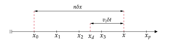
Figure 2: Schematic of the interpolation process and the collocation points during the semi-Lagrangian advection.

The advecton equation (26) is recast in the following form

$$f_{i}^{\lambda}(x,t)=\sum_{p=0}^{N-1}l_{p}\mathcal{M}_{i,\lambda}^{-1}M^{*}(x_{p},t-\delta t),$$ (198)

where $l_{p}$ are the interpolation weights. At this point, no explicit type of the interpolation function is assumed and the weights $l_{p}$ or their properties remain to be derived. Considering that $x_{p}=x-(n-p)\delta x$, one can expand Eq. (198) using the Taylor series up to third-order terms

$$f_{i}(x,t) =\sum_{p}l_{p}\mathcal{M}_{i}^{-1}\left(M^{*}(x,t)-\delta t\bar{D}_{p}M^{*}(x,t)+\frac{\delta t^{2}}{2}\bar{D}_{p}^{2}M^{*}(x,t)\right)$$

$$=f_{i}^{*}(x,t)\sum_{p}l_{p}-\delta t\mathcal{M}_{i}^{-1}\sum_{p}l_{p}\bar{D}_{p}M^{*}(x,t)$$

$$+\frac{\delta t^{2}}{2}\mathcal{M}_{i}^{-1}\sum_{p}l_{p}\bar{D}_{p}^{2}M^{*}(x,t),$$ (199)

where $\bar{D}_{p}=\partial_{t}+(n-p)(\delta x/\delta t)\partial_{x};\ p=0:N-1$.

In the following, we shall compute the individual terms in Eq. (199). In order to be consistent, any interpolation scheme requires the weights to sum to unity, i.e.

$$\sum_{p}l_{p}=1.$$ (200)

The other terms are computed as follows

$$\sum_{p}l_{p}\bar{D}_{p}M^{*}=\bar{D}_{0}M^{*}-\sum_{p}l_{p}p\frac{\delta x}{\delta t}\partial_{x}M^{*},$$ (201)

$$\sum_{p}l_{p}\bar{D}^{2}_{p}M^{*} =\bar{D}^{2}_{0}M^{*}+\left(\sum_{p}l_{p}p^{2}-2n\sum_{p}l_{p}p\right)\frac{\delta x^{2}}{\delta t^{2}}\partial_{xx}M^{*}$$

$$-2\sum_{p}l_{p}p\frac{\delta x}{\delta t}\partial_{xt}M^{*},$$ (202)

In a moment-conserving interpolation function Koumoutsakos (1997); van Rees (2014), we have the property

$$\sum_{p}l_{p}(p\delta x)^{r}=(x_{d}-x_{0})^{r},$$ (203)

where the number of conserved moments $r$ depends on the order of the interpolation function. Hence, we require the interpolation scheme to obey the property (203) with $r=2$ at least. This implies that a stencil with a minimum of three points must be used for the interpolation.

Substituting Eq. (203) in Eqs. (201) and (202) leads to

$$\sum_{p}l_{p}\bar{D}_{p}M^{*}=\partial_{t}M^{*}+v_{i}\partial_{x}M^{*}=D_{i}M^{*},$$ (204)

$$\sum_{p}l_{p}\bar{D}^{2}_{p}M^{*} =\partial_{tt}M^{*}+2v_{i}\partial_{xt}M^{*}+v_{i}^{2}\partial_{xx}M^{*}$$

$$=D^{2}_{i}M^{*}-D_{i}v_{i}\partial_{x}M^{*}.$$ (205)

It can be simplify verified that once the averaged terms (204) and (205) are plugged in Eq. (199), the kinetic equation of the continuous case (39) is recovered. Therefore, all the analysis presented so far are also valid when the interpolation procedure is included provided that the interpolation function encompasses three support points at least and abides the moment-conserving property.

III.6 Prandtl number

In section III.4, it was shown that the choice of equilibrium for the second population for a standard lattice such as $D2Q9$ will affect the recovered energy equation. Beside the unwanted error terms, the Prandtl number obtained by the Chapman-Enskog analysis will be a rational function of the specific heat, i.e. Eq. (197), if only the extra internal energy is assigned to the second population $(\phi=1)$. On the other hand, choosing $\phi=0$ will remove the error terms and recover ${\rm Pr}=1$. Moreover, we illustrated that in order to have a consistent scheme, the interpolation function must feature a moment conserving property with at least three support points.

To verify our analysis, we conduct the standard test case to measure the value of the Prandtl number Dorschner et al. (2018). We choose the $D2Q9$ lattice with the first-order $(N=2,r=1)$, second-order $(N=3,r=2)$ and third-order $(N=4,r=3)$ Lagrange interpolation schemes. Figure 3 shows that our analysis are consistent with the simulations. It is also clearly visible that the interpolation scheme with $r<2$ deviates from the underlying theoretical values.

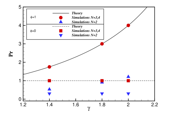
Figure 3: The measured Prandtl number against the adiabatic exponent using the $D2Q9$ lattice and different values of $\phi$.

III.7 Convergence study

The standard LBM is a second-order accurate scheme in space and time featuring $\delta x=\delta t=1$. On the other hand, it is well-known that the compressibility errors in the standard LBM scale with ${\rm Ma}^{2}$ and the NSE is recovered with error terms proportional to ${\rm Kn}^{2}$, where $\rm Kn$ is the Knudsen number Krüger et al. (2017). However, it has been shown that the semi-Lagrangian LBM (SLLBM) Krämer et al. (2017); Wilde et al. (2020b) can achieve higher orders by decoupling the time step from the grid spacing provided that the time step (or CFL) and the Mach number is kept relatively low. Then, high-order interpolation functions can lead to high spatial order of accuracy. In this case, as shown and discussed in Wilde et al. (2020b); Krämer et al. (2020), the discretization errors are in the order of $\mathcal{O}({\rm min}(\delta x^{N}/\delta t,\delta x^{N-1}))$. On the other hand, we have shown that using 9 discrete velocities in the PonD framework will introduce error terms in the order of $\mathcal{O}(\delta t)$ in the momentum and energy equations. Finally, one can summarize that the present model include error terms as deviations from the full compressible NSE, which are in the order of

$$D1Q3,D2Q9:$$

$$\mathcal{O}\left({\rm min}\left(\frac{\delta x^{N}}{\delta t},\delta x^{N-1}\right),\delta t,{\rm Kn}^{2}\right),$$

$$D1Q5,D2Q25:$$

$$\mathcal{O}\left({\rm min}\left(\frac{\delta x^{N}}{\delta t},\delta x^{N-1}\right),\delta t^{2},{\rm Kn}^{2}\right),$$ (206)

where the compressibility error $\mathcal{O}(\rm Ma^{2})$ is eliminated thanks to the exact equilibrium function. In the following, we will assess the validity of these results by conducting numerical simulations. To verify the spatial discretization errors, a density profile is advected with the following initial conditions

$$\rho_{0}(x)=1+\exp(-300(x-0.5)^{2}),\ 0\leqslant x\leqslant 1,$$

$$p_{0}(x)=1,$$

$$u_{0}(x)=1.$$ (207)

While the number of grid points $Nx$ are varied in this simulation, the time step is fixed at a small value $\delta t=10^{-4}$ to eliminate the chance of dominance of temporal errors. A third-order Lagrange interpolation function with four support points is adopted in this simulation and the value of the specific heat is chosen as $\gamma=1.4$. We let the simulations run until $t=1$, which corresponds to one period in time. To reflect the maximum error throughout the domain, the $L_{\infty}$-error defined as

$$L_{\infty}=\max\left(\left|\frac{\rho(x)-\rho_{0}(x)}{\rho_{0}(x)}\right|\right)$$ (208)

is measured to investigate the error convergence.

Figure 4 shows that the underlying order of accuracy of the interpolation function is recovered for both $D2Q25$ and $D2Q9$ lattices and is independent of the choice of the equilibrium function for the second population, as expected.

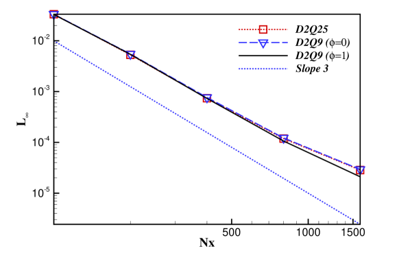
Figure 4: Convergence of the $L_{\infty}$ error in the linear advection test: all schemes recover the underlying order of accuracy.

Figure 5 shows the local Mach number for number of grid points $N=400$. It is noticed that the range of the Mach number in this simulation is significantly high, whereas it was shown that the compressibility errors in SLLBM Krämer et al. (2017) can already prevail at ${\rm Ma}=0.1$. This is due to the Galilean-invariant nature of the PonD model where it eliminates the compressibility errors by designing particles at the co-moving reference frame and the exact collision seen from those particles

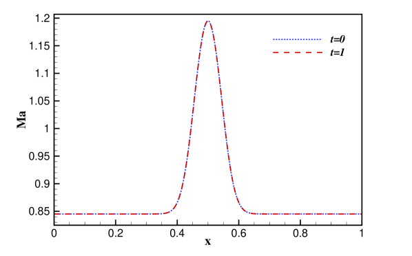
Figure 5: Mach profile of the linear advection test at $\delta t=10^{-4}$, using the $D2Q9$ lattice, ${\color[rgb]{0,0,0}Nx}=400$ and $\phi=0$.

To study the behavior of the temporal errors, we simulate the advection of a vortex by a uniform flow at ${\rm Ma}_{a}=U_{a}/\sqrt{\gamma T_{0}}=0.845$ Frapolli et al. (2016a). The velocity field in the cylindrical coordinates and in the advected reference frame is $u_{\theta}(r)=u_{\rm max}r\exp[(1-r^{2})/2]$, where $r=r^{\prime}/R$ is the reduced radius and $R$ is the radius of the vortex. The vortex Mach number is defined based on the maximum tangential velocity in the co-moving reference frame, ${\rm Ma}_{v}=u_{\rm max}/\sqrt{\gamma T_{0}}$ and is fixed to ${\rm Ma}=0.4$. The Reynolds number is fixed to ${\rm Re}=2U_{a}R/\nu=6\times 10^{5}$ and a $400\times 400$ grid is used. The vortex is allowed to complete one cycle of rotation during one period of advection and then the x-velocity component is measured along the centerline, where its deviation from the exact solution is indicative of errors. This simulation is repeated with different timesteps with a fixed advection velocity.

Figure 6 shows the $L_{\infty}$ errors for both the $D2Q25$ and $D2Q9$ lattices. We see the results are recovered consistently with Eq. (206), where the $D2Q25$ lattice shows second-order convergence, while the $D2Q9$ lattice is first-order in time when the excess internal energy is assigned to the $g$ population, i.e. $\phi=1$. Another interesting point, which rises in this simulation is the non-monotonic behavior of the temporal errors in the $D2Q25$ lattice. This is due to the competing effect between the $\mathcal{O}(\delta x^{N}/\delta t)$ and $\mathcal{O}(\delta t^{2})$ error terms, when the resolution $\delta x$ and the order of the interpolation $N$ are fixed. Depending on their orders of magnitude, the latter might take over at small time steps and increase the errors as time is refined. At first, a second-order convergence is observed until $U_{a}\delta t/\delta x=0.5$. After this point, further refinement results in increasing the errors implying that the $\mathcal{O}(\delta x^{N}/\delta t)$ term has become dominant. This reverse effect, which was also reported in Wilde et al. (2020b) is not observed in the $D2Q9$ lattice in this setup since the $\mathcal{O}(\delta t)$ terms retain greater magnitude throughout the refinement procedure.

As said earlier, the choice of $\phi$ can affect the recovered energy equation when the $D2Q9$ lattice is used, such that $\phi=0$ can remove the errors from the energy equation. However, the momentum equation will still have the $\mathcal{O}(\delta t)$ errors and the scheme will be effectively first-order in time. To verify this, we augment the post-collision $f$ populations by a forcing term as

$$f_{i}^{*}(\bm{x},t)=f_{i}(\bm{x},t)+\omega(\rho w_{i}-f_{i})_{(\bm{x},t)}+\hat{f}_{i}\delta t,$$ (209)

where $\hat{f}_{i}=\mathcal{M}^{-1}_{i}\bm{X}$ and

$$\bm{X}=[0,X_{xM},X_{yM},0,0,0,0,0,0]^{\dagger},$$ (210)

includes the error terms in the momentum equation recovered in (164).

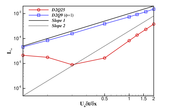
Figure 6: Time refinement study in the simulation of advected vortex: convergence of the $L_{\infty}$ error by decreasing the timestep. $400\times 400$ grid points are used.

Choosing $\phi=0$ and forcing out the error terms $X_{\alpha M}$, we repeat the same simulation using the $D2Q9$ lattice. As demonstrated in Fig. 7, the scheme becomes second-order accurate in time once the error terms are corrected. This indicates that the analysis are consistent with simulations.

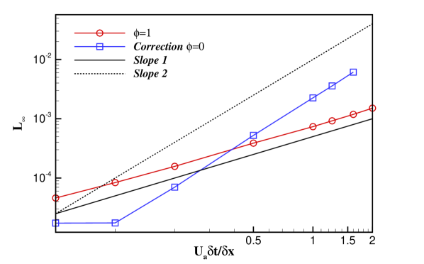
Figure 7: Time refinement study in the simulation of advected vortex: convergence of the $L_{\infty}$ error by decreasing the timestep. The $D2Q9$ lattice is used with $\phi=1$ and $\phi=0$ augmented by the correction term.

IV Benchmark

In this section, the interaction of a vortex with a standing shock front is considered. The Mach number of the vortex is ${\rm Ma}_{v}=0.25$ and its radius is denoted by $R_{v}$. When passing through the shock front with the intensity ${\rm Ma}_{a}=1.2$, sound waves are generated by the vortex. To assess the numerical accuracy of a model, one can measure the sound pressure and compare to the DNS solution INOUE and HATTORI (1999). In this simulation, the Reynolds number is defined as ${\rm Re}=a_{\infty}R_{v}/\nu$, where $a_{\infty}$ is the speed of sound upstream of the shock and the dimensionless time $t^{*}=ta_{\infty}/R_{v}$ is used. Figure 8 shows the radial sound pressure measured from the center of the vortex along the $\theta=-45^{\circ}$ line with respect to the $x$ axis. The results are captured at three different times for ${\rm Re}=800$ and ${\rm Pr}=0.75$.

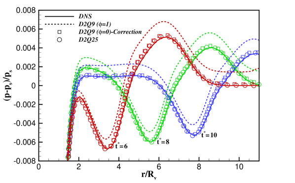
Figure 8: Radial sound pressure measured at $\theta=-45^{\circ}$ with respect to the $x$ axis at nondimensional times $t^{*}=\{6,8,10\}$. The governing parameters are ${\rm Ma}_{a}=1.2,{\rm Ma}_{v}=0.25,{\rm Re}=800$ and ${\rm Pr}=0.75$. DNS from INOUE and HATTORI (1999).

Compared to the DNS solution, one observes that the $D2Q9$ lattice overestimates the pressure, while removing the error terms ($\phi=0$ and adding the correction term) leads to a significant improvement such that the latter together with the $D2Q25$ lattice are in good agreement with the DNS solution.

V Conclusion

In this paper, a consistent analysis of the particles on demand kinetic model was presented. Due to the off-lattice property of the model, the semi-Lagrangian advection is used, which requires interpolation schemes. In our Chapman-Enskog analysis, we have taken into account the effect of the interpolation and transformation of populations during the advection process. By doing so, we have derived the hydrodynamic limit of the model for commonly used one and two-dimensional lattices. It has been demonstrated that the $D2Q9$ lattice in the PonD framework have error terms in the order of timestep in the momentum and energy equations, while the $D2Q25$ lattice can recover the full compressible NSE. However, the error terms corresponding to the energy equation recovered from the $D2Q9$ lattice could be eliminated by adopting a second population to carry the total energy instead of the excess internal energy.

Furthermore, we discussed that similar to other semi-Lagrangian LB schemes, the spatial order of accuracy can be increased by employing high-order interpolation functions at low CFL numbers. However, the compressibility errors are no longer present thanks to the Galilean-invariant nature of the model.

As for the validation, the presented analysis were verified on various numerical benchmarks. It was shown that the results were improved upon including corrections to remove the error terms.

Finally, we comment that the current analysis can be applied to three-dimesnional lattices. In the case of tensor-product lattices such as $D3Q27$ and $D3Q125$, the recovered equations for fluid properties such as viscosity, conductivity and Prandtl number will be the same as their two-dimensional counterpart (Eqs. (160)-(162), (169), (194)). However, for any general lattice, a separate investigation must be carried out due to their unique form of mapping matrix.

VI Acknowledgement

The author thanks I. Karlin and B. Dorschner for the discussions.

Appendix A

In this section, we aim to analyze the predictor-corrector step during the advection process. To this end, we take the $D1Q3$ lattice with the inverted mapping matrix $\mathcal{M}^{-1}$ as shown by Eq. (53). For simplicity, the interpolation kernel is once again neglected. The goal is to find the co-moving gauge at point $x$ and time $t_{0}+\delta t$ assuming that the flow variables are known at time $t_{0}$. As explained in section III.1, the particles at point $x$ are first set relative to the initial gauge $\lambda_{0}=\lambda(x,t_{0})$. Hence the initial value of the discrete velocities are

$$v_{i}^{0}=v_{i}(x,t_{0})=\sqrt{\theta_{0}}c_{i}+u_{0},$$ (211)

where $\theta_{0}=\theta(x,t_{0})$ and $u_{0}=u(x,t_{0})$. At the next step, the semi-Lagrangian advection is followed using Eq. (36)

$$f_{i}^{\lambda_{0}}=\mathcal{M}_{i,\lambda_{0}}^{-1}M^{*}(x-v_{i}^{0}\delta t,t_{0}).$$ (212)

Consequently, using Eqs. (30)-(32), the updated density, momentum and total energy values are obtained and denoted as $\rho_{1},(\rho u)_{1},(2\rho E)_{1}$, respectively.
In general, one can express the populations at the $n$th iteration by

$$f_{i}^{\lambda_{n}}=\mathcal{M}_{i,\lambda_{n}}^{-1}M^{*}(x-v_{i}^{n}\delta t,t_{0}),$$ (213)

where $\lambda_{n}=\{T_{n},u_{n}\}$ denotes the reference frame corresponding to the computed temperature $T_{n}=\theta_{n}T_{\rm{L}}$ and velocity $u_{n}$. The flow variables are updated as

$$\rho_{n+1} =\sum_{i}f_{i}^{\lambda_{n}},$$ (214)

$$(\rho u)_{n+1} =\sum_{i}f_{i}^{\lambda_{n}}v_{i}^{n},$$ (215)

$$(2\rho E)_{n+1} =\sum_{i}f_{i}^{\lambda_{n}}{v_{i}^{n}}^{2}.$$ (216)

It is straightforward to show

$$f_{0}^{\lambda_{n}} =\left(1-\frac{u_{n}^{2}}{\theta_{n}}\right)\rho(x_{0}^{n})+\frac{2u_{n}}{\theta_{n}}(\rho u)(x_{0}^{n})-\frac{1}{\theta_{n}}(2\rho E)(x_{0}^{n}),$$

$$f_{1}^{\lambda_{n}} =\frac{u_{n}^{2}-\sqrt{\theta_{n}}u_{n}}{2\theta_{n}}\rho(x_{1}^{n})+\frac{\sqrt{\theta_{n}}-2u_{n}}{2\theta_{n}}(\rho u)(x_{1}^{n})+\frac{1}{2\theta_{n}}(2\rho E)(x_{1}^{n}),$$

$$f_{2}^{\lambda_{n}} =\frac{u_{n}^{2}+\sqrt{\theta_{n}}u_{n}}{2\theta_{n}}\rho(x_{2}^{n})-\frac{\sqrt{\theta_{n}}+2u_{n}}{2\theta_{n}}(\rho u)(x_{2}^{n})+\frac{1}{2\theta_{n}}(2\rho E)(x_{2}^{n}),$$ (217)

where $x_{j}^{n};j=0,1,2$ are the departure points as shown in Fig. 1, at the $n$th iteration, such that

$$x_{0}^{n} =x-u_{n}\delta t,$$

$$x_{1}^{n} =x-\sqrt{\theta_{n}}\delta t-u_{n}\delta t,$$

$$x_{2}^{n} =x+\sqrt{\theta_{n}}\delta t-u_{n}\delta t.$$ (218)

It can be observed that $x_{0}^{n}$ is always the middle point between $x_{1}^{n}$ and $x_{2}^{n}$. Note that the moments $[\rho,\rho u,2\rho E]$ in Eq. (217) – evaluated at departure points $x_{j}^{n}$ – are known from the previous time step $t=t_{0}$. It must be commented that the transformation process is not positivity preserving, i.e. the transformed populations can assume negative values depending on the target reference frame (see Eq. (217).
Before proceeding further, we use Taylor series to expand these terms around $(x,t_{0})$ up to third order accuracy. Finally, taking the first two moments of 217, we have

$$\rho_{n+1} =\rho(x,t_{0})-\delta t\partial_{x}(\rho u)+\frac{\delta t^{2}}{2}\partial_{xx}(2\rho E)+\mathcal{O}(\delta t^{3}),$$ (219)

$$(\rho u)_{n+1} =(\rho u)(x,t_{0})+\frac{\delta t^{2}}{2}u_{n}^{3}\partial_{xx}\rho-\frac{\delta t^{2}}{2}u_{n}\theta_{n}\partial_{xx}\rho$$

$$-\frac{3}{2}\delta t^{2}u_{n}^{2}\partial_{xx}(\rho u)+\frac{\delta t^{2}}{2}\theta_{n}\partial_{xx}(\rho u)-\delta t\partial_{x}(2\rho E)$$

$$+\frac{3}{2}\delta t^{2}u_{n}\partial_{xx}(2\rho E)$$ (220)

It is observed that the evaluated density during the iterations is independent of its previous values (there is no dependence on $\rho_{n}$). Hence, one can write $\rho=\rho_{n}=\rho_{n+1}$. For further simplification, assume the isothermal condition, i.e., $\theta_{n}=1$. According to Eq. (220), the difference of computed momentums between two subsequent iterations is

$$\rho(u_{n+1}-u_{n}) =\frac{\delta t^{2}}{2}(u_{n}^{3}-u_{n-1}^{3})\partial_{xx}\rho-\frac{\delta t^{2}}{2}(u_{n}-u_{n-1})\partial_{xx}\rho$$

$$-\frac{3}{2}\delta t^{2}(u_{n}^{2}-u_{n-1}^{2})\partial_{xx}(\rho u)$$

$$+\frac{3}{2}\delta t^{2}(u_{n}-u_{n-1})\partial_{xx}(2\rho E).$$ (221)

It is straightforward to show that

$$\left|\frac{u_{n+1}-u_{n}}{u_{n}-u_{n-1}}\right|=\mathcal{O}(\delta t^{2}).$$ (222)

Hence, the predictor-corrector algorithm is always convergent at relatively low time steps.

Another approach is to evaluate the derivative of the iteration function. According to the fixed-point iteration method, the iterative process $x_{n+1}=\Psi(x_{n})$ will be convergent if $|\Psi^{\prime}(x)|<1$ for a specified interval.
Rearranging Eq. (221) as $u_{n+1}=\Psi(u_{n})$, it can be shown that

$$\left|\frac{\partial\Psi}{\partial u}\right|=\mathcal{O}(\delta t^{2}).$$ (223)

References

- Succi (2018) S. Succi, The lattice Boltzmann equation: for complex states of flowing matter (Oxford University Press, 2018).
- Krüger et al. (2017) T. Krüger, H. Kusumaatmaja, A. Kuzmin, O. Shardt, G. Silva, and E. M. Viggen, Springer International Publishing 10, 4 (2017).
- Sbragaglia et al. (2006) M. Sbragaglia, R. Benzi, L. Biferale, S. Succi, and F. Toschi, Physical Review Letters 97, 204503 (2006).
- Biferale et al. (2012) L. Biferale, P. Perlekar, M. Sbragaglia, and F. Toschi, Physical Review Letters 108, 104502 (2012), arXiv:1111.0905 .
- Benzi et al. (2009) R. Benzi, S. Chibbaro, and S. Succi, Physical Review Letters 102, 026002 (2009).
- Mazloomi M et al. (2015) A. Mazloomi M, S. S. Chikatamarla, and I. V. Karlin, Physical Review Letters 114, 174502 (2015).
- Kunert and Harting (2007) C. Kunert and J. Harting, Physical Review Letters 99, 176001 (2007), arXiv:0705.0270 .
- Hyväluoma and Harting (2008) J. Hyväluoma and J. Harting, Physical Review Letters 100, 246001 (2008), arXiv:0801.1448 .
- Atif et al. (2017) M. Atif, P. K. Kolluru, C. Thantanapally, and S. Ansumali, Phys. Rev. Lett. 119, 240602 (2017).
- Dorschner et al. (2016) B. Dorschner, F. Bösch, S. S. Chikatamarla, K. Boulouchos, and I. V. Karlin, Journal of Fluid Mechanics 801, 623 (2016).
- Pirozzoli (2011) S. Pirozzoli, Annual review of fluid mechanics 43, 163 (2011).
- Wilde et al. (2020a) D. Wilde, A. Krämer, D. Reith, and H. Foysi, Physical Review E 101, 053306 (2020a), arXiv:1910.13918 .
- Feng et al. (2019) Y. Feng, P. Boivin, J. Jacob, and P. Sagaut, Journal of Computational Physics 394, 82 (2019).
- Frapolli et al. (2015) N. Frapolli, S. S. Chikatamarla, and I. V. Karlin, Physical Review E - Statistical, Nonlinear, and Soft Matter Physics 92, 061301 (2015).
- Prasianakis and Karlin (2008) N. I. Prasianakis and I. V. Karlin, Physical Review E - Statistical, Nonlinear, and Soft Matter Physics 78, 016704 (2008).
- Frapolli et al. (2016a) N. Frapolli, S. S. Chikatamarla, and I. V. Karlin, Physical review letters 117, 10604 (2016a).
- Frapolli et al. (2016b) N. Frapolli, S. S. Chikatamarla, and I. V. Karlin, Physical Review E 93, 63302 (2016b).
- Chikatamarla and Karlin (2006) S. S. Chikatamarla and I. V. Karlin, Physical review letters 97, 190601 (2006).
- Dorschner et al. (2018) B. Dorschner, F. Bösch, and I. V. Karlin, Physical Review Letters 121, 130602 (2018), arXiv:1806.05089 .
- He and Luo (1997) X. He and L.-S. Luo, Phys. Rev. E 56, 6811 (1997).
- Ansumali and Karlin (2005) S. Ansumali and I. V. Karlin, Phys. Rev. Lett. 95, 260605 (2005).
- Koumoutsakos (1997) P. Koumoutsakos, Journal of Computational Physics 138, 821 (1997).
- van Rees (2014) W. M. van Rees, 3D simulations of vortex dynamics and biolocomotion, Ph.D. thesis, ETH Zurich (2014).
- Krämer et al. (2017) A. Krämer, K. Küllmer, D. Reith, W. Joppich, and H. Foysi, Physical Review E 95, 23305 (2017).
- Wilde et al. (2020b) D. Wilde, A. Krämer, D. Reith, and H. Foysi, Physical Review E 101, 53306 (2020b).
- Krämer et al. (2020) A. Krämer, D. Wilde, K. Küllmer, D. Reith, H. Foysi, and W. Joppich, Computers & Mathematics with Applications 79, 34 (2020).
- INOUE and HATTORI (1999) O. INOUE and Y. HATTORI, Journal of Fluid Mechanics 380, 81–116 (1999).