Permutation Binary Neural Networks: Analysis of Periodic Orbits and Its Applications

Abstract.

This paper presents a permutation binary neural network characterized by local binary connection, global permutation connection, and the signum activation function. The dynamics is described by a difference equation of binary state variables. Depending on the connection, the network generates various periodic orbits of binary vectors. The binary/permutation connection brings benefits to precise analysis and to FPGA based hardware implementation. In order to consider the periodic orbits, we introduce three tools: a composition return map for visualization of the dynamics, two feature quantities for classification of periodic orbits, and an FPGA based hardware prototype for engineering applications. Using the tools, we have analyzed all the 6-dimensional networks. Typical periodic orbits are confirmed experimentally.

Hotaka Udagawa, Taiji Okano and Toshimichi Saito^∗

Department of Electrical and Electronic Engineering, HOSEI University

Koganei, Tokyo, 184-8584, Japan

1. Introduction

Discrete-time recurrent-type neural networks have been studied actively in both viewpoints of nonlinear dynamics and engineering applications [1]-[4]. The networks are characterized by real valued connection parameters and nonlinear activation functions. The dynamics is described by autonomous difference equations of real valued state variables. Even in the low-dimensional cases, the networks can exhibit various periodic/chaotic phenomena [4]-[6]. Several effective synthesis methods have been presented for applications such as associative memories [1]-[4], combinatorial optimization problems solvers [7], and reservoir computing [8]. In the recurrent-type neural networks, fixed points have been studied sufficiently. For example, parameter conditions for existence/stability of fixed points are presented and are applied to storage of stable desired memories into the associative memories [1]-[3]. However, analysis of periodic orbits is difficult and has not been studied sufficiently. The difficulty is caused by huge parameter space, curse of dimensionality and complex nonlinear dynamics. In order to realize the analysis, a simple mathematical model with a variety of periodic orbits is necessary.

This paper presents a permutation binary neural network (PBNN) and considers classification/stability of periodic orbits. The PBNN is a simple recurrent-type neural network characterized by local binary connection parameters, global permutation connection parameters, and the signum activation function. The dynamics is described by an $N$-dimensional autonomous difference equation of binary state variables. Depending on the parameters and initial conditions, the PBNN generates various periodic orbits of binary vectors (BPOs). Engineering applications of the BPOs include control signal of switching power converters [22] and control signal of walking robots [23]-[25]. The PBNNs can be regarded as a simplified version of dynamic binary neural networks (DBNNs [9]-[13]) characterized by global ternary connection. If the permutation connection does not exist, the PBNNs are equivalent to elementary cellular automata [14]-[19] governed by rules of linearly separable Boolean functions. The binary/permutation connection brings benefits to precise analysis of dynamics and to simple hardware implementation based on a field-programmable gate array (FPGA) [20] [21].

In order to consider the PBNNs and their BPOs, we present three tools. The first tool is a composition return map (Cmap) for visualization of the dynamics. The Cmap is a composition of two maps. The first map represents the local binary connection and the second map represents the global permutation connection. The second tool is two feature quantities for classification of PBNNs. Roughly speaking, the first feature quantity evaluates complexity of the BPOs and the second feature quantity evaluates stability of the BPOs. Using the two feature quantities, a feature plane is constructed on which PBNNs are classified based on their BPOs. The third tool is an FPGA based hardware prototype for engineering applications. Using the tools, we have considered all the 6-dimensional PBNNs whose parameter space consists of ($8\times 6!$) points. The dynamics is visualized in Cmap on $2^{6}$ points where we can grasp BPOs and transient phenomena. The BPOs from the PBNNs are classified on the feature plane where we can see that the global permutation connection makes various BPOs. Using the standard design procedure, the PBNNs are implemented on an FPGA board and typical BPOs are confirmed experimentally. These results provide basic information to realize more detailed analysis of PBNNs and its applications.

It should be noted that this is the first paper of the PBNN and analysis of its BPOs. The Cmap is a developed version of the digital return maps [9] for DBNNs without the concept of composition. Design of the FPGA based hardware prototype is based on simple Boolean functions and is applicable to hardware implementation of the elementary cellular automata.

2. Two related systems

As background of the PBNNs, we introduce elementary cellular automata (ECAs [14]-[18]) and dynamics binary neural networks (DBNNs, [9]-[13]). In various discrete-time dynamical systems, these two systems are simple and exhibit various BPOs.

2.1. Elementary cellular automata

We introduce the ECAs defined on a ring of $N$ cells. Let $x_{i}^{t}\in\{-1,+1\}\equiv\bm{B}$ be the $i$-th binary state at discrete time $t$. The dynamics is described by the $N$-dimensional autonomous difference equation:

$$x^{t+1}_{i}=F(x^{t}_{i-1},x^{t}_{i},x^{t}_{i+1}),\ \ i\in\{1,\cdots,N\},\ N\geq 3$$ (1)

where $x_{0}^{t}\equiv x_{N}^{t}$ and $x_{N+1}^{t}\equiv x_{1}^{t}$ for ring-type connection. A Boolean function $F$ transforms three binary inputs into one binary output. Fig. 1 shows an example:

$$\begin{array}[]{llll}F(-1,-1,-1)=-1&F(-1,-1,1)=-1&F(-1,1,-1)=1&F(-1,1,1)=-1\\ F(1,-1,-1)=1&F(1,-1,1)=-1&F(1,1,-1)=1&F(1,1,1)=1\end{array}$$

Decimal expression of the 8 outputs is referred to as the rule number (RN). In this example, the 8 outputs $(-1-1+1-1+1-1+1+1)\equiv(00101011)_{2}=212_{10}$ is declared as RN212. There exist $2^{2^{3}}=256$ rules in the ECAs and the rules are characterized by the $\lambda-$parameter = (the number of output +1)/8. The RN212 is characterized by $\lambda=0.5$. Depending on the rules and initial conditions, the ECAs can generate various sequences of binary vectors (BPOs and transient phenomena) as studied in [14]-[16]. Engineering applications are many, including information compression [17], reservoir computing [18], and error correcting code [19]. Analysis of the ECAs is important from both viewpoints of nonlinear dynamics and engineering applications.

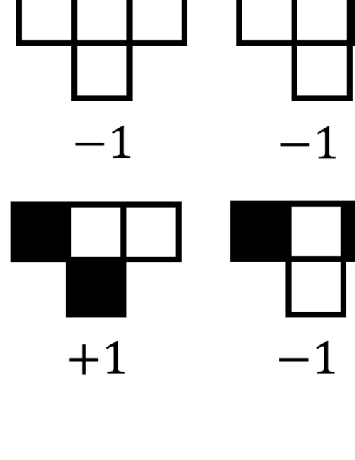
Figure 1. An example of 6-dimensional ECA (RN212) and a sequence of binary vectors. Black and white squares denote output $+1$ and $-1$, respectively.

2.2. Dynamic binary neural networks

The DBNNs are recurrent-type neural networks described by the $N$-dimensional autonomous difference equation of binary state variables:

$$\begin{array}[]{c}\displaystyle x_{i}^{t+1}=\mbox{sgn}\left(\sum_{j=1}^{N}w_{ij}x_{j}^{t}-T_{i}\right)\ i\in\{1,\cdots,N\},\ N\geq 3\\ \mbox{sgn}(X)=\left\{\begin{array}[]{ll}+1&\mbox{for }X\geq 0\\ -1&\mbox{for }X<0\end{array}\right.\end{array}$$ (2)

where $x_{i}^{t}\in\bm{B}$ is the $i$-th binary state at discrete time $t$. The DBNNs are characterized by ternary connection parameters $w_{ij}\in\{-1,0,+1\}$ and the signum activation function. The threshold parameters $T_{j}$ are integer. Depending on the parameters and initial conditions, the DBNNs can generate various BPOs. In [9], we have considered storage and stabilization of special BPOs for application to switching power converters. In [10], we have analyzed the DBNNs with special sparse connection and have given theoretical results for storage and stabilization of rotation-type BPOs. However, in these DBNNs, storage of any BPO is not guaranteed. In [11], we have presented three-layer DBNNs and a simple parameter setting method that guarantees storage of any BPO. However, the number of hidden neurons increases in proportional to the period of BPOs. The three-layer DBNNs have been implemented in an FPGA board and have been applied to controlling hexapod walking robots [12] [13].

2.3. Problems in ECAs and DBNNs

Although BPOs are simpler than real valued periodic orbits, it is not easy to analyze BPOs in DBNNs and ECAs. Connection parameter space of the DBNNs is huge. The ECAs and DBNNs exhibit complicated dynamics as $N$ increases.

3. Permutation Binary Neural Networks and Identifier

We presents the PBNN and consider BPOs from the PBNN. First, we introduce a simple binary neural network (SBNN) corresponding to the input to hidden layers in the PBNN. The SBNN is characterized by local binary connection and the signum activation function. The dynamics is described by the following $N$-dimensional autonomous difference equation of binary state variables:

$$x_{i}^{t+1}=\mbox{sgn}\left(w_{a}x_{i-1}^{t}+w_{b}x_{i}^{t}+w_{c}x_{i+1}^{t}\right),\ i\in\{1,\cdots,N\},\ N\geq 3$$ (3)

where $x_{i}^{t}\in\bm{B}$ is the $i$-th binary state variable at discrete time $t$. As shown in Fig. 2(a), $x_{N+1}^{t}\equiv x_{1}^{t}$ and $x_{0}^{t}\equiv x_{N}^{t}$ for ring-type connection. The local binary connection is determined by three binary valued connection parameters $w_{a}\in\bm{B}$, $w_{b}\in\bm{B}$, and $w_{c}\in\bm{B}$. Depending on the parameters, the signum activation function $\mbox{sgn}(X)$ constructs a linearly separable Boolean function from three binary inputs $(x^{t}_{i-1},x^{t}_{i},x^{t}_{i+1})$ to one binary output $x_{i}^{t+1}$. Note that $X\in\{-3,-1,+1,+3\}$ for $X\equiv w_{a}x_{i-1}^{t}+w_{b}x_{i}^{t}+w_{c}x_{i+1}^{t}$. In order to identify the local binary connection, we introduce connection number (CN)

$$\begin{array}[]{cc}\mbox{CN0 for }(w_{a},w_{b},w_{c})=(-1,-1,-1)&\mbox{(RN23)}\\ \mbox{CN1 for }(w_{a},w_{b},w_{c})=(-1,-1,+1)&\mbox{(RN43)}\\ \mbox{CN2 for }(w_{a},w_{b},w_{c})=(-1,+1,-1)&\mbox{(RN77)}\\ \mbox{CN3 for }(w_{a},w_{b},w_{c})=(-1,+1,+1)&\mbox{(RN142)}\\ \mbox{CN4 for }(w_{a},w_{b},w_{c})=(+1,-1,-1)&\mbox{(RN113)}\\ \mbox{CN5 for }(w_{a},w_{b},w_{c})=(+1,-1,+1)&\mbox{(RN178)}\\ \mbox{CN6 for }(w_{a},w_{b},w_{c})=(+1,+1,-1)&\mbox{(RN212)}\\ \mbox{CN7 for }(w_{a},w_{b},w_{c})=(+1,+1,+1)&\mbox{(RN232)}\end{array}$$ (4)

The 8 CNs corresponding to 8 Boolean function of 8 RNs of ECAs as shown in Eq. (4). Fig. 2 (a) shows Example 1: A 6-dimensional SBNN of CN6. Depending on initial conditions, this SBNN exhibits sequences of binary vectors including a BPO with period 6 as shown in the figure. All the 8 rules are characterized by $\lambda$-parameter=0.5.

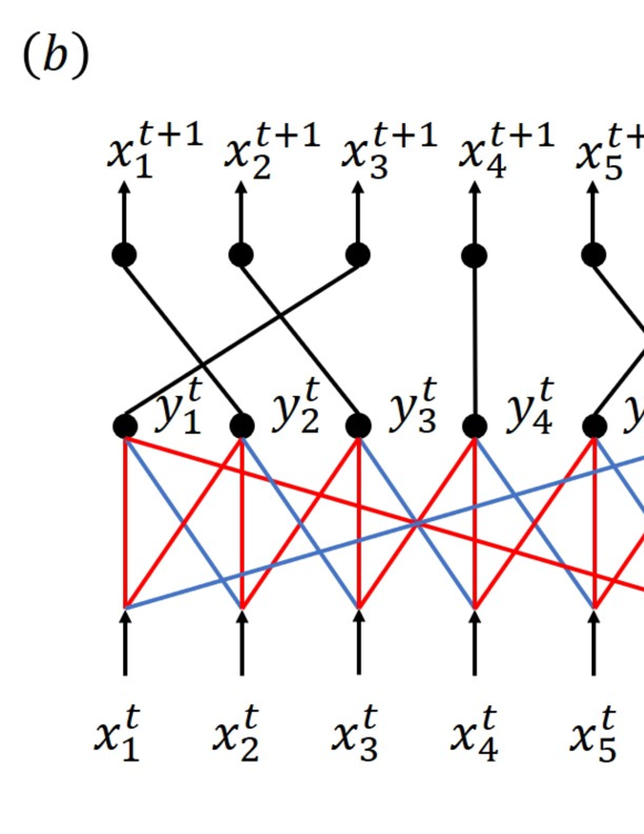
Figure 2. Networks and BPOs. (a) SBNN in Example 1. Red and blue branches denote positive and negative connections, respectively. (b) PBNN in Example 2 (CN6, P231465). Black branches denote permutation connection.

Adding global permutation connection from hidden to output layer, the PBNN is constructed. The dynamics is described by the following $N$-dimensional autonomous difference equation of binary state variables:

$$\begin{array}[]{l}x_{i}^{t+1}=y_{\sigma(i)}^{t}\\ y_{i}^{t}=\mbox{sgn}\left(w_{a}x_{i-1}^{t}+w_{b}x_{i}^{t}+w_{c}x_{i+1}^{t}\right)\end{array}\ \ \sigma=\left(\begin{array}[]{cccc}1&2&\cdots&N\\ \sigma(1)&\sigma(2)&\cdots&\sigma(N)\end{array}\right)$$ (5)

where $y_{i}^{t}\in\bm{B}$ is the $i$-th binary hidden state and $\sigma$ is a permutation. Let $\bm{x}^{t}\equiv(x_{1}^{t},\cdots,x_{N}^{t})$ and let $\bm{y}^{t}\equiv(y_{1}^{t},\cdots,y_{N}^{t})$. The local binary connection (from input to hidden layers) transforms an binary input vector $\bm{x}^{t}$ into the binary hidden vector $\bm{y}^{t}$. The global permutation connection (from hidden to output layers) transforms the $\bm{y}^{t}$ into the binary output vector $\bm{x}^{t+1}$. Fig. 2 (b) shows Example 2: A 6-dimensional PBNN given by

$$(w_{a},w_{b},w_{c})=(+1,+1,-1)\ \ \ \mbox{(CN6)},\ \sigma=\left(\begin{array}[]{cccccc}1&2&3&4&5&6\\ 2&3&1&4&6&5\end{array}\right)\ \ \mbox{(P231465)}$$ (6)

As shown in the figure, this PBNN exhibits a BPO with period 12 where a BPO with period $p$ is defined by

$$\bm{z}^{1},\cdots,\bm{z}^{p},\cdots\ \ \left\{\begin{array}[]{ll}\bm{z}^{t_{1}}=\bm{z}^{t_{2}}&\mbox{for }|t_{2}-t_{1}|=np\\ \bm{z}^{t_{1}}\neq\bm{z}^{t_{2}}&\mbox{for }|t_{2}-t_{1}|\neq np\end{array}\right.$$ (7)

where $\bm{z}^{t}=(z_{1}^{t},\cdots,z_{N}^{t})$, $z_{i}^{t}\in\bm{B}$ and $n$ denotes positive integers. In Example 2, the local binary connection is the same as the connection of SBNN in Example 1: applying the global permutation connection to the SBNN of BPO with period 6, we obtain the PBNN that generates BPO with period 12. Effects of the permutation connection is discussed in Section 5. In order to identify the global permutation connection, we introduce permutation identifier P$\sigma(1)\cdots\sigma(N)$. In Example 2, the PBNN is identified by CN6 and P231465. In general, a PBNN is identified by connection number the CN and the permutation identifier. Here, we have described the parameter space of a PBNN clearly: the parameter subspace of a SBNN consists of 8 points represented by the 8 connection numbers (CNs), the parameter subspace of the permutation consists of $N!$ permutation identifiers, and the parameter space of a PBNN consists of the $8\times N!$ points represented by the CN and the permutation identifier. The binary/permutation connection parameters bring benefits in precise analysis and simple FPGA based hardware implementation.

4. Tools for numerical analysis

4.1. Tool 1: Composition digital return map

In order to visualize the dynamics of PBNNs, we present the Tool 1: composition digital return map (Cmap). The Cmap is a composition of the 1st map $f_{1}$ for local binary connection (SBNN) and the 2nd map $f_{2}$ for global permutation connection. First, we introduce the 1st map $f_{1}$ for the SBNN. The domain and range of the SBNN are the set of all the $N$-dimensional binary vectors $\bm{B}^{N}$. The $\bm{B}^{N}$ is equivalent to a set of $2^{N}$ points $L_{N}\equiv\{c_{1},\cdots,c_{2^{N}}\}$, e. g., $C_{1}\equiv(-1,\cdots,-1)$, $C_{2}\equiv(+1.-1.\cdots,-1)$, $\cdots$, $C_{2^{N}}\equiv(+1,\cdots,+1)$. The dynamics of the SBNN is integrated into

$$\mbox{1st map: }\bm{x}^{t+1}=f_{1}(\bm{x}^{t}),\ \bm{x}^{t}\in\bm{B}^{N}\equiv L_{D}$$ (8)

Here we give basic definition for the 1st map.

Definition 1: A point $\bm{z}_{p}\in L_{D}$ is said to be a binary periodic point (BPP) with period $p$ if $f^{p}(\bm{z}_{p})=\bm{z}_{p}$ and $f_{1}(\bm{z}_{p})$ to $f_{1}^{p}(\bm{z}_{p})$ are all different where $f_{1}^{k}$ is the $k$-fold composition of $f_{1}$. A sequence of the BPPs, $\{f_{1}(\theta_{p}),\cdots,f_{1}^{p}(\theta_{p})\}$, is said to be a BPO with period $p$. A point $\bm{z}_{e}$ is said to be an eventually periodic point (EPP) if $\bm{z}_{e}$ is not a BPP but falls into a BPO, i.e., there exists some positive integer $l$ such that $f_{1}^{l}(\bm{z}_{e})$ is a BPP.

Fig. 3 (a) shows the 1st map consisting of $2^{6}$ points for the 6-dimensional SBNN in Example 1. The 1st map exhibits a BPO with period 6 as shown in Fig. 3 (b) corresponding to the BPO with period 6 in Fig. 2 (a). In the figure, several EPPs are also shown.

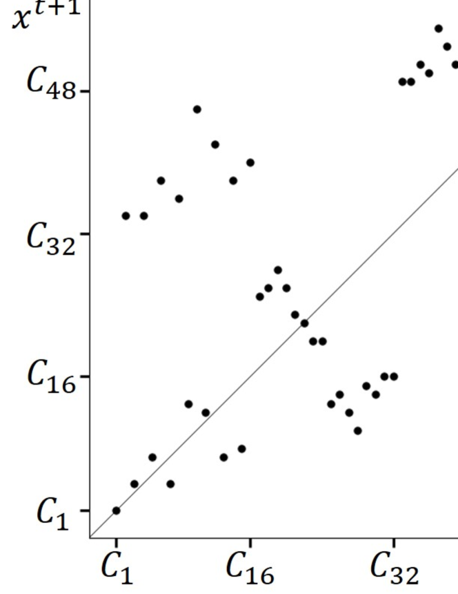
Figure 3. 1st map $f_{1}$ for SBNN, CN6. (a) 1st map of 64 points. (b) BPO(red) with period 6 and EPPs (green).

Next, we introduce the 2nd map $f_{2}$. In the PBNN, the binary hidden state vector $\bm{y}^{t}\in\bm{B}^{N}$ is transformed into the binary output vector $\bm{x}^{t+1}\in\bm{B}^{N}$ via permutation $\sigma$. The transformation is integrated into

$$\mbox{2nd map: }\bm{x}^{t+1}=f_{2}(\bm{y}^{t}),\ \bm{y}^{t}\in\bm{B}^{N}\equiv L_{D}.$$ (9)

The dynamics of the PBNN is integrated into a composition map (Cmap) of the 1st and the 2nd maps:

$$\mbox{Cmap: }\bm{x}^{t+1}=f(\bm{x}^{t})\equiv f_{2}(f_{1}(\bm{x}^{t})),\ \bm{x}^{t}\in\bm{B}^{N}\equiv L_{D}$$ (10)

Fig. 4 shows the Cmap for the 6-dimensional PBNN in Example 2: composing the 1st map in Fig. 4(a) and 2nd map in Fig. 4(b), we obtain the Cmap in Fig. 4 (c). The 1st map visualizes dynamics of the 6-dimsnsional SBNN in Fig. 2 (a), the 2nd map visualizes global permutation connection P231465, and the Cmap visualizes dynamics of the 6-dimensional PBNN in Fig. 2 (b). The Cmap exhibits multiple BPOs including the BPO with period 12 as shown in Fig. 4 (d). This figure suggests that the global permutation connection is effective to realize a variety of BPOs. The BPO, BPP, and EPP of the Cmap are defined by replacing the 1st map $f_{1}$ with the Cmap $f$ in Definition 1.

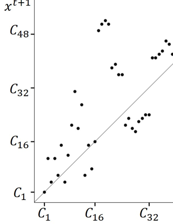
Figure 4. Cmaps for PBNN. (a) The 1st map $f_{1}$ for CN6. (b) The 2nd map $f_{2}$ for P231465. (c) Cmap $f$ of 64 points. (d) BPO with period 12 (red) and EPPs (green). BPO with period 4 (blue).

4.2. Tool 2: Feature quantities

In order to classify PBNNs by their BPOs, we present the Tool 2: two simple feature quantities. As shown in the Cmap in Fig. 4 (d), the PBNN can have multiple BPOs and exhibits one of them depending on the initial points. Since analysis of multiple BPOs is not easy, we consider one BPO with the maximum period (MBPO). In Example 2, the BPO with period 12 is the MBPO as shown in Fig. 4(d). The first feature quantity is defined by

$$\alpha=\mbox{(The period of MBPO)}/2^{N},\ \frac{1}{2^{N}}\leq\alpha\leq 1.$$ (11)

As $\alpha$ increase, the MBPO approaches the M-sequence. Roughly speaking, the quantity $\alpha$ evaluates complexity of the MBPO.

The second feature quantity is defined by

$$\beta=\mbox{(The number of initial points falling into the MBPO)}/2^{N},\ \alpha\leq\beta\leq 1.$$ (12)

Note that the initial points consist of BPPs in the MBPO and EPPs to the MBPO: $\alpha\leq\beta$. The difference $(\beta-\alpha)$ is proportional to the number of EPPs that evaluates stability of the MBPO. In order not to disturb existence of EPPs, the period should not be too long, e.g., $\alpha\leq 1/3$. Note that the stability corresponds to bit error correction capability in digital dynamical systems and corresponds to basin of attraction in analog dynamical systems [6]. As $\beta$ increases, the stability becomes stronger. If multiple MBPOs exist, one MBPO with larger $\beta$ is adopted.

Using the two feature quantities, we construct a feature plane as shown in Fig. 5. In the figure, SBNN in Example 1 is represented by a point $(\alpha,\beta)=(6/64,12/64)$ and PBNN in Example 2 is represented by a point $(\alpha,\beta)=(12/64,40/64)$. The permutation (P231465) increases both $\alpha$ and $\beta$.

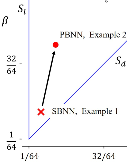
Figure 5. Feature plane and three segments $S_{d}$, $S_{t}$, and $S_{l}$. Red cross: SBNN, Example 1 ($\alpha=6/64$, $\beta=12/64$). Red circle: PBNN, Example 2 ($\alpha=12/64$, $\beta=40/64$).

As stated earlier, as $\alpha$ increases, period of the MBPO becomes longer (more complex). As $(\beta-\alpha)$ increases, stability of the MBPO becomes stronger. A PBNN is represented by its MBPO and the MBPO gives one point in the feature plane. The point exists in a triangle surrounded by the three segments each of which has the following meaning.

• $S_{d}(\alpha=\beta)$: There exists no EPP to the MBPO and no transient phenomenon to the MBPO.

• $S_{t}(\beta=1)$: All the initial points fall into the MBPO and the PBNN has unique BPO=MBPO.

• $S_{l}(\alpha=1/2^{N})$: The MBPO is a fixed point (BPO with period 1).

The feature plane is useful for basic classification of PBNNs.

5. Numerical analysis

Using the Tool 1 and Tool 2, we analyze PBNNs. Since analysis of $N$-dimensional PBNNs is not easy, we consider 6-dimensional PBNNs in this paper. The case $N=6$ is convenient in the following three points. First, the case $N=6$ is applicable to engineering systems such as hexapod walking robots [13] and power converters with 6 switches [9]. Second, in the 6-dimensional PBNNs, the number of points in the parameter space (parameter values) is $8\times 6!=5760$ and the brute force attack is possible to calculate Cmaps and feature quantities. The 5760 points is much smaller than $3^{6^{2}}$ points in the parameter space of the 6-dimensional DBNNs in Eq. (2). An effective calculation method for BPOs and EPPs can be found in [26]. As $N$ increases, the number of elements in the domain $\bm{B}^{N}\equiv L_{N}$ increases exponentially and we must use an evolutionary computation algorithm etc. Third, the Cmap consists of $2^{N}=2^{6}$ points and is visible. As $N$ increases, the number of points increases exponentially and the Cmap is hard to inspect.

Fig. 6 shows 1st maps with MBPOs for all the 8 SBNNs. As stated earlier, the SBNNs correspond to 8 ECAs governed by 8 rules of $\lambda$-parameter 0.5. In CN6, the MBPO with period 6 is applicable to control signal of hexapod robots [13]. Using the two feature quantities, MBPOs of the 8 SBNNs are evaluated:

$$\begin{array}[]{lll}\mbox{CN0}:(w_{a},w_{b},w_{c})=(-1,-1,-1)&\alpha=2/64&\beta=32/64\\ \mbox{CN1}:(w_{a},w_{b},w_{c})=(-1,-1,+1)&\alpha=6/64&\beta=12/64\\ \mbox{CN2}:(w_{a},w_{b},w_{c})=(-1,+1,-1)&\alpha=2/64&\beta=2/64\\ \mbox{CN3}:(w_{a},w_{b},w_{c})=(-1,+1,+1)&\alpha=6/64&\beta=12/64\\ \mbox{CN4}:(w_{a},w_{b},w_{c})=(+1,-1,-1)&\alpha=6/64&\beta=12/64\\ \mbox{CN5}:(w_{a},w_{b},w_{c})=(+1,-1,+1)&\alpha=2/64&\beta=32/64\\ \mbox{CN6}:(w_{a},w_{b},w_{c})=(+1,+1,-1)&\alpha=6/64&\beta=12/64\\ \mbox{CN7}:(w_{a},w_{b},w_{c})=(+1,+1,+1)&\alpha=2/64&\beta=2/64\end{array}$$

Dynamics of all the 8 SBNNs are visualized in the 8 1st maps in Fig. 6 corresponding to all the 8 points in the parameter space. The SBNNs exhibit MBPOs with period 6 and MBPOs with period 2.

Applying global permutation connection to each SBNN of local binary connection, we obtain PBNNs that can generate MBPO with longer period than that of SBNN. Fig. 7 shows Cmaps of a typical PBNN for each SBNN. Using the two feature quantities, MBPOs of the 8 PBNNs are evaluated:

$$\begin{array}[]{llll}\mbox{CN0}:\mbox{P513246}&\alpha=8/64&\beta=20/64\\ \mbox{CN1}:\mbox{P413625}&\alpha=20/64&\beta=62/64\\ \mbox{CN2}:\mbox{P524361}&\alpha=10/64&\beta=36/64\\ \mbox{CN3}:\mbox{P315462}&\alpha=20/64&\beta=62/64\\ \mbox{CN4}:\mbox{P254136}&\alpha=20/64&\beta=62/64\\ \mbox{CN5}:\mbox{P461253}&\alpha=10/64&\beta=62/64\\ \mbox{CN6}:\mbox{P126354}&\alpha=20/64&\beta=62/64\\ \mbox{CN7}:\mbox{P651324}&\alpha=8/64&\beta=20/64\\ \end{array}$$ (13)

Dynamics of the 8 PBNNs are visualized in 8 Cmaps in Fig. 6. In these examples, four PBNNs give the MBPO with the maximum period 20 ($\alpha=20/64$) and the strongest stability ($\beta=62/64$). In each PBNN, the global permutation connection realizes longer period than each SBNN.

Next, applying the brute force attack to all $6!=720$ PBNNs for each SBNN, we have calculated the two feature quantities. The results are summarized in the feature plane in Fig. 8. In each feature plane, the red cross corresponds to the SBNN of the 1st map in Fig. 6 and the red circle corresponds to the PBNN of the Cmap in Fig. 7. The PBNN of the red circle has the MBPO with the longest period ($\alpha$) and the strongest stability ($\beta$) for the longest period. We can see that the global permutation connection is effective to increase the period and stability of MBPOs. Note that points of CN1 and CN4 (respectively, CN3 and CN6) are the same and the points are distributed in wide range: the global permutation connection is effective to generate a variety of MBPOs. In CN2 and CN5, $\alpha$ distributes in a narrow range whereas $\beta$ distributes in a wide range. In CN0 and CN7, both $\alpha$ and $\beta$ distributes in a relatively narrow range: the local binary connection $w=(-1,-1,-1)$ or $(+1,+1,+1)$ seems not to make a variety of BPOs. These results from 6-dimansional PBNNs suggest huge variety of BPOs and hardness of analysis in the higher-dimensional PBNNs. Note that, in Fig. 8, the parameter space of the PBNNs is classified into 8 subspaces (8 CNs). On each parameter subspace, the two feature quantities are distributed and the typical values are red marked. These results provide basic information to consider relationship between the feature quantities and the parameters. The parameters are represented by the permutation identifier and connection number (CN).

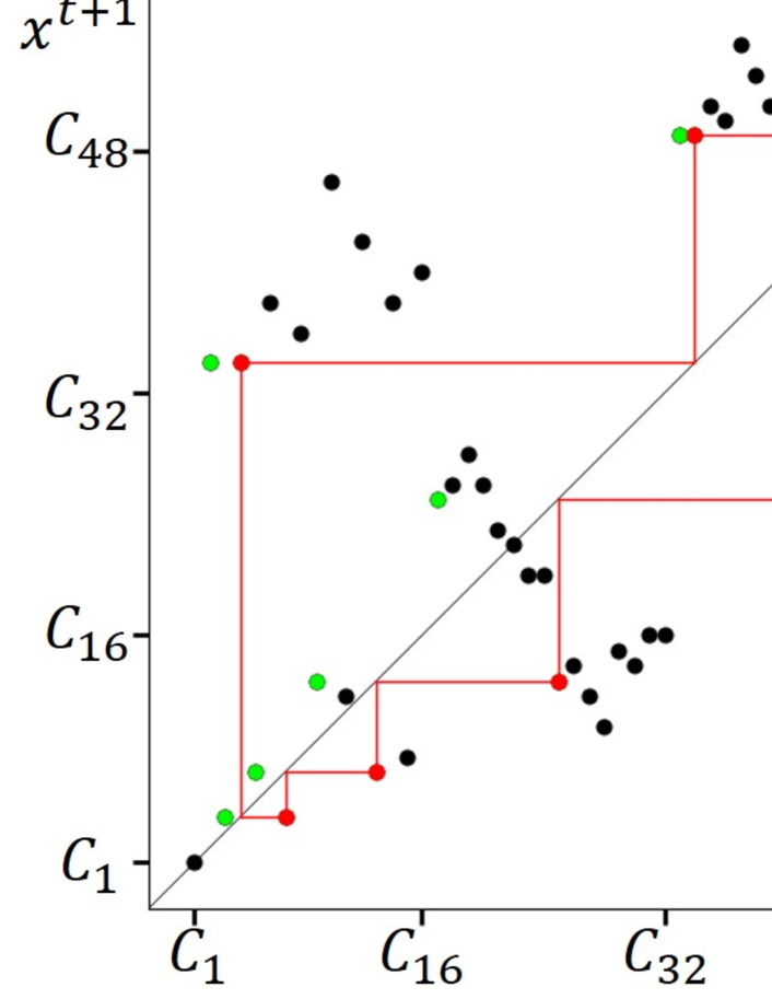
Figure 6. 1st map of 8 SBNNs with MBPO (red) and EPPs (green).

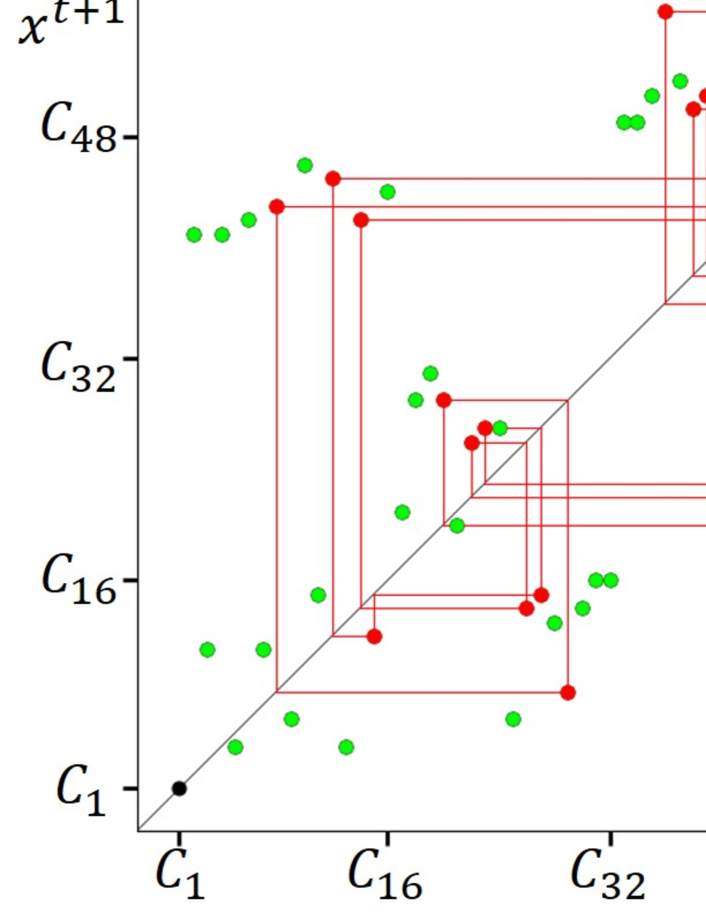
Figure 7. Cmap of PBNNs with MBPO (red) and EPPs (green). CN0: P513246. CN1: P413625. CN2: P524361. CN3: P315462. CN4: P254136. CN5: P461253. CN6: P126354. CN7: P651324.

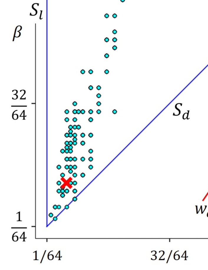
Figure 8. Feature planes. Red cross: SBNN, Red circle: PBNN in Fig. 7. CN0(19 points). CN1(79). CN2(49). CN3(78). CN4(79). CN5(53). CN6(78). CN7(26).

It should be noted that, on each feature plane, the number of points is less than the number of PBNNs. For example, on the feature plane of CN6, 78 points exist for 720 PBNNs. Multiple PBNNs give the same value of the two future quantities $\alpha$ and $\beta$. For more detailed classification, novel feature quantities are necessary.

6. Tool 3: FPGA based hardware

In order to realize engineering applications, we present the Tool 3: an FPGA based hardware prototype. The FPGA is an integrated circuit designed to be configured by a designer after manufacturing. The advantages include high speed/precision operation and high degree of integration [20] [21]. We have designed the hardware and have measured typical BPOs in the following environment.

• Verilog version: Vivado 2018.2 platform (Xilinx).

• FPGA: BASYS3 (Xilinx Artix-7 XC7A35T-ICPG236C).

• Clock: 10[MHz]. The default frequency 100[MHz] is divided for clear measurements.

• Measuring instrument: ANALOG DISCOVERY2.

• Multi-instrument software: Waveforms 2015

Algorithms 1 and 2 show SystemVerilog codes for hardware design. In the Algorithm 1, as a connection number CN (equivalent to a rule number RN) is given, the corresponding Boolean function is obtained and the SBNN is realized. This design strategy is based on the Boolean functions from three input to one output and is applicable to implementation of ECAs for all the 256 rules. In Algorithm 2, as a permutation identifier is given, the global permutation connection is realized. Applying these two algorithms, a desired PBNN is realized. Varying the CN and permutation identifier, we obtain a desired PBNN in $8\times N!$ PBNNs.

Using the algorithms, the SBNN and PBNN are implemented on the FPGA board. Fig. 10(a) shows measured waveform of MBPO1 with period 6 form the SBNN in Fig. 2 (a). The MBPO1 is applicable to control signal of hexapod walking robots and the control strategy can be found in [13]. Fig. 10(b) shows measured waveform of MBPO2 with period 20 corresponding to the Cmap in Fig. 7 CN6. The MBPO2 has the longest period that is impossible in 6-dimensional SBNNs. This FPGA prototype provides basic information to realize engineering applications of 6 or higher dimensional PBNNs.

Algorithm 1 SBNN

  module SBNN(parameter $N=6$)

  (output reg $x[1:N]$,

  reg $[1:N]x^{t+1}$);

  wire $rule0,rule1,\cdots,rule7;$

  parameter RN = 8’b212 ; // Rule Number

  genvar $j$;

  for$(j=1;j<=N;j=j+1)$begin

      assign $rule0=RN[0]^{\ast}($~$x[j-1]\ \&\$~$x[j]\ \&\$~$x[j+1]);$ // Boolean function

      assign $rule1=RN[1]^{\ast}($~$x[j-1]\ \&\$~$x[j]\ \&\ x[j+1]);$

      assign $rule2=RN[2]^{\ast}($~$x[j-1]\ \&\ x[j]\ \&\$~$x[j+1]);$

      assign $rule3=RN[3]^{\ast}($~$x[j-1]\ \&\ x[j]\ \&\ x[j+1]);$

      assign $rule4=RN[4]^{\ast}(x[j-1]\ \&\$~$x[j]\ \&\$~$x[j+1]);$

      assign $rule5=RN[5]^{\ast}(x[j-1]\ \&\$~$x[j]\ \&\ x[j+1]);$

      assign $rule6=RN[6]^{\ast}(x[j-1]\ \&\ x[j]\ \&\$~$x[j+1]);$

      assign $rule7=RN[7]^{\ast}(x[j-1]\ \&\ x[j]\ \&\ x[j+1]);$

      assign $x^{t+1}[j]=(rule0)|(rule1)|~{}...~{}|(rule7);$

  end

  endmodule

Algorithm 2 PBNN

  module PBNN(parameter $N=6$)

  (input clk,load,rst,

  input $i[1:N],$

  output reg $x[1:N]$);

  reg $[1:N]x^{t+1}$;

  integer $k$;

  integer $y[1:N]=[1,2,6,3,5,4];$ // Permutation identifier P126354

  always $@$(posedge clk)begin

    if(load$==1$)begin

      for$(k=1;k<=N;k=k+1)$begin

        $x[k]=i[k];$ // Initial condition

      end

    end else if(rst$==1$)begin

      for$(k=1;k<=N;k=k+1)$begin

        $x[k]=0;$

      end

    end else begin

      for$(k=1;k<=N;k=k+1)$begin

        $x[k]=x^{t+1}[y[k]];$ // Permutation

      end

    end

  end

  SBNN SBNN$(x,x^{t+1})$;

  endmodule

7. Conclusions

The PBNNs and the three tools are presented in this paper: the Cmap for visualization of the dynamics, the two feature quantities for basic classification of PBNNs, and the FPGA based hardware prototype for engineering applications. Using the tools, all the 6-dimensionl PBNNs have been analyzed and typical MBPOs are confirmed experimentally. In our future works, we should consider various problems including the following. 1. Relation between permutation identifier and feature quantities. 2. Application of the global permutation to ECAs of 256 rules and analysis of the dynamics. 3. Novel feature quantities for more detailed classification of PBNNs. 4. Evolutionary algorithms for analysis and synthesis of higher-dimensional PBNNs. 5. Engineering applications of the FPGA based hardware.

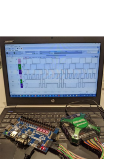
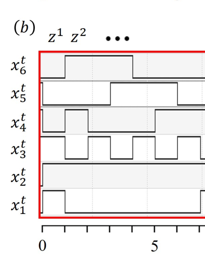
Figure 9. Experimental setup: FPGA and Analog discovery.

Figure 10. Measured waveforms of MBPOs in the FPGA board. (a) MBPO1 with period 6 from SBNN CN6. (b) MBPO2 with period 20 from PBNN CN6 P126354.

References

- [1] [10.1073/pnas.79.8.2554] J. J. Hopfield, \doititleNeural networks and physical systems with emergent collective computation abilities, Proc. Nat. Acad. Sci., 79 (1982), 2554-2558.
- [2] [10.1109/37.55118] A. N. Michel and J.A. Farrell, \doititleAssociative memories via artificial neural networks, IEEE Control Systems Magazine, 10 (1990) 6-17.
- [3] [10.1109/31.62410] A. N. Michel, J.A. Farrell and H. F. Sun, \doititleAnalysis and synthesis techniques for Hopfield type synchronous discrete time neural networks with application to associative memory, IEEE Trans. Circuits Systs., 37 (1990), 1356-1366.
- [4] [10.1016/S0893-6080(96)00061-5] M. Adachi and K. Aihara, \doititleAssociative dynamics in a chaotic neural network, Neural Networks, 10 (1997), 83-98.
- [5] [10.1038/261459a0] R. May, \doititleSimple mathematical models with very complicated dynamics, Nature, 261 (1976), 259-467.
- [6] E. Ott, Chaos in dynamical systems, Cambridge, 1993.
- [7] [10.1007/BF00339943] J. J. Hopfield and D. W. Tank, \doititle‘Neural’ computation of decisions optimization problems, Biological Cybern., 52 (1985), 141-152.
- [8] [10.1038/ncomms1476] L. Appeltant, M. C. Soriano, G. Van der Sande, J. Danckaert, S. Massar, J. Dambre, B. Schrauwen, C. R. Mirasso and I. Fischer, \doititleInformation processing using a single dynamical node as complex system, Nat. Commun., 2 (2011), Article number: 468.
- [9] [10.1016/j.neucom.2016.10.084] R. Sato and T. Saito, \doititleStabilization of desired periodic orbits in dynamic binary neural networks, Neurocomputing, 248 (2017), 19-27.
- [10] [10.1016/j.neucom.2019.03.015] S. Aoki, S. Koyama and T. Saito, \doititleTheoretical analysis of dynamic binary neural networks with simple sparse connection, Neurocomputing, 341 (2019), 149-155.
- [11] [10.1016/j.neucom.2020.01.105] S. Koyama and T. Saito, \doititleGuaranteed storage and stabilization of desired binary periodic orbits in three-layer dynamic binary neural networks, Neurocomputing, 416 (2020), 12–18.
- [12] [10.1016/j.neucom.2021.06.054] S. Anzai, T. Suzuki and T. Saito, \doititleDynamic binary neural networks with time-variant parameters and switching of desired periodic orbits, Neurocomputing, 457 (2021), 357–364.
- [13] [10.1109/CNNA49188.2021.9610809] T. Suzuki and T. Saito, \doititleSynthesis of three-layer dynamic binary neural networks for control of hexapod walking robots, Proc. IEEE/CNNA (2021).
- [14] S. Wolfram, Cellular automata and complexity: collected papers, CRC Press, 2018.
- [15] [10.1142/6014-vol1] L. O. Chua, A nonlinear dynamics perspective of Wolfram’s new kind of science I, World Scientific, 2006.
- [16] [10.1063/1.4771662] M. Schüle and R. Stoop, \doititleA full computation-relevant topological dynamics classification of elementary cellular automata, Chaos, 22 (2012), 043143, 10pp.
- [17] (MR1975953) [10.1016/S0375-9601(01)00610-7] W. Wada, J. Kuroiwa and S. Nara, \doititleCompletely reproducible description of digital sound data with cellular automata, Phys. Lett. A, 306 (2002), 110–115.
- [18] [10.1162/NECO_a_00787] O. Yilmaz, \doititleSymbolic computation using cellular automata-based hyperdimensional computing, Neural Computation, 27 (2015), 2661–2692.
- [19] [10.1109/12.286310] D. R. Chowdhury, S. Basu, I. S. Gupta and P. Chaudhuri, \doititleDesign of CAECC - cellular automata based error correcting code, IEEE Trans. Comput., 43-6 (1994), 756–764.
- [20] https://www.intel.com/content/www/us/en/artificial-intelligence/programmable/overview.html
- [21] [10.3934/dcdss.2020374] H. Uchida, Y. Oishi and T. Saito, \doititleA simple digital spiking neural network: synchronization and spike-train approximation, Discrete Contin. Dyn. Syst. Ser. S., 14 (2021), 1479–1494.
- [22] [10.1109/TNN.2007.899181] W. Holderbaum, \doititleApplication of neural network to hybrid systems with binary inputs, IEEE Trans. Neural Netw., 18 (2007), 1254–1261.
- [23] [10.1109/TNNLS.2019.2945637] M. Lodi, A. L. Shilnikov and M. Storace, \doititleDesign principles for central pattern generators with preset rhythms, IEEE Trans. Neural Netw. Learn. Syst., 31 (2020), 3658–3669.
- [24] [10.1109/TNNLS.2020.3016523] M. Thor, T. Kulvicius and P. Manoonpong, \doititleGeneric neural locomotion control framework for legged robots, IEEE Trans. Neural Netw. Learn. Syst., 32 (2021), 4013–4025.
- [25] [10.1007/s11071-019-05028-z] P. Arena, L. Patané and A. G. Spinosa, \doititleA nullcline-based control strategy for PWL-shaped oscillators, Nonlinear Dyn., 97 (2019), 1011-1033.
- [26] [10.1587/nolta.3.596] N. Horimoto and T. Saito, \doititleAnalysis of digital spike maps based on bifurcating neurons, NOLTA, IEICE, 3 (2012), 596–605.
- [27] [10.1016/j.neunet.2021.08.034] E. J. Schiessler, R. C. Aydin, K. Linka and C. J. Cyron, \doititleNeural network surgery: Combining training with topology optimization, Neural Networks, 144 (2021), 384-393.