Prescribed Performance Adaptive Fixed-Time Attitude Tracking Control of a 3-DOF Helicopter with Small Overshoot

Abstract

In this article, a novel prescribed performance adaptive fixed-time backstepping control strategy is investigated for the attitude tracking of a 3-DOF helicopter. First, a new unified barrier function (UBF) is designed to convert the prescribed performance constrained system into an unconstrained one. Then, a fixed-time (FxT) backstepping control framework is established to achieve the attitude tracking. By virtual of a newly proposed inequality, a non-singular virtual control law is constructed. In addition, a FxT differentiator with a compensation mechanism is employed to overcome the matter of “explosion of complexity”. Moreover, a modified adaptive law is developed to approximate the upper bound of the disturbances. To obtain a less conservative and more accurate approximation of the settling time, an improved FxT stability theorem is proposed. Based on this theorem, it is proved that all signals of the system are FxT bounded, and the tracking error converges to a preset domain with small overshoot in a user-defined time. Finally, the feasibility and effectiveness of the presented control strategy are confirmed by numerical simulations.

I Introduction

In recent decades, as one of the typical rotorcrafts, the helicopter has been paid substantial attention because of its widespread applications in various scenarios [1]. However, the high-performance tracking control design of the helicopter remains a challenging project due to the characteristics of the system [2].

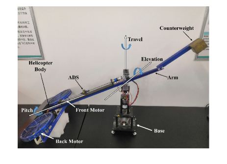
Figure 1: Structure of the 3-DOF helicopter system

Owing to the advantages of high tracking accuracy, fast response, and anti-interference capability, finite-time (FnT) control approaches have become a research hotspot [3]. Recently, a variety of FnT control schemes have been developed and applied to the 3-DOF helicopter platform (Fig. 1). In [4], a robust regulation controller for the laboratory helicopter was constructed based on the super-twisting sliding mode observer (STSMO), which was utilized to estimate the lumped disturbances and identify the state vector in finite time. To tackle the problem that the upper bound of disturbance is usually unknown in advance, the authors in [5] developed an adaptive-gain super-twisting algorithm for the tracking control of the helicopter platform. In [6], an adaptive FnT control law based on a continuous differentiator was presented for the lab helicopter system, which can effectively suppress chattering. An adaptive smooth FnT control protocol, integrated with a singularity-free integral sliding mode surface, was established to fulfill the helicopter attitude tracking in [7]. In [8], a novel control strategy, which embraced a modified FnT backstepping controller based on a newly designed disturbance observer, was presented for the tracking problem of the lab helicopter platform.

The drawback of the above strategies is that the settling time is related to the initial conditions, which is difficult to obtain accurately in many practical systems. Moreover, when the initial states are far from the equilibrium points, the settling time will become longer. To work out this problem, the FxT stability was first put forward in [9], where the settling time has no connection with the initial values. Thereafter, numerous FxT control approaches were developed to solve the control problems of different kinds of systems [10, 11, 12, 13].

Although the above-mentioned control laws can fulfill the satisfactory steady-state performance, the tracking errors’ transient behavior is seldom taken into account. For the sake of addressing this problem, a prescribed performance control approach was first presented in [14], which introduced the concepts of error transformation and performance function (PF) to guarantee the behavior at both transient and steady states. In [15], the FnT prescribed tracking control was achieved by means of a newly designed PF. Authors in [16] proposed a novel prescribed performance FxT control scheme to realize the guaranteed tracking of strict-feedback nonlinear systems. By incorporating the PF with backstepping algorithm, a FxT adaptive control protocol was developed in [17] to cope with the trajectory tracking problem. In addition, a FxT differentiator with a novel auxiliary compensator was adopted to handle the “explosion of complexity”.

Enlightened by the aforementioned observations, this article develops a novel prescribed performance adaptive fixed-time control protocol for the attitude tracking of the 3-DOF helicopter system via the backstepping algorithm. First, a newly designed UBF is utilized to transform the prescribed performance constrained system into an unconstrained one. Then, motivated by [17], a FxT backstepping control strategy is established to fulfill the attitude tracking. By using a newly proposed inequality, a non-singular virtual control law is constructed. In addition, a FxT differentiator with a compensator is adopted to overcome the matter of “explosion of complexity”. To compensate the impact of disturbances, a modified adaptive law is developed. The major innovations of this article can be stated as follows:

1. A novel UBF is developed to convert the prescribed performance restrained system into an unrestrained one, which can effectively diminish the control input by selecting appropriate parameters.

2. An improved FxT stability theorem is proposed to provide a less conservative and more accurate approximation of the settling time than the classical result.

Based on the modified FxT stability theorem, it is proved that all signals of the system are FxT bounded, while the tracking error converges to a predetermined domain with small overshoot in a user-defined time. The feasibility and effectiveness of the proposed control protocol are confirmed by numerical simulations.

The rest of this article is arranged as follows. The mathematical model of the helicopter system, an improved FxT stability theorem and some useful lemmas are presented in Section II. Section III describes the control design procedure. Numerical simulations are conducted in Section V to show the feasibility and effectiveness of the designed control protocol. Section VI draws the conclusion.

Notation: In this article, ${\mathop{\rm sig}\nolimits}{\left(x\right)^{r}}={\left|x\right|^{r}}{\mathop{\rm sgn}}(x)$.

II Problem formulation and preliminaries

II-A Problem Formulation

In light of the attitude tracking problem of elevation and pitch angles, the mathematical model of the helicopter system can be expressed as [7]

$${{\dot{x}}_{1}} ={x_{2}}$$ (1)

$${{\dot{x}}_{2}} =\frac{{{L_{a}}}}{{{J_{\alpha}}}}{{\bar{u}}_{1}}-\frac{g}{{{J_{\alpha}}}}m_{e}{L_{a}}\cos({x_{1}})+{d_{1}}(x,t)$$

$${{\dot{x}}_{3}} ={x_{4}}$$

$${{\dot{x}}_{4}} =\frac{{{L_{h}}}}{{{J_{\beta}}}}{{\bar{u}}_{2}}+{d_{2}}(x,t)$$

The definitions of variables and the values of parameters can be found in [7].

The control aim is to design a prescribed performance FxT control protocol such that the tracking errors can converge to a predetermined domain with small overshoot in a user-defined time, while all signals of the system are bounded within a fixed time.

Assumption 1

The desired tracking signals ${x_{1d}}(t),{x_{3d}}(t)$ and their derivatives are bounded, smooth and known.

Assumption 2

The disturbances are bounded as well as smooth.

II-B Improved FxT stability

Lemma 1

Consider the following system

$$\dot{x}(t)=f(x(t)),x(0)={x_{0}}$$ (2)

where $x\in{R^{n}}$, $f:{R^{n}}\to{R^{n}}$ and $f(0)=0$. If there exists a continuous Lyapunov function $V\left(x\right)$ satisfying:

$$\dot{V}(x(t))\leq-{\mu_{1}}V{(x(t))^{p}}-{\mu_{2}}V{(x(t))^{q}}{\rm{+}}{\mu_{3}}$$ (3)

where ${\mu_{1}}>0,{\mu_{2}}>0,0<{\mu_{3}}<\infty,0<p<1,q>1$, then the origin of system (2) is practical FxT stable, and the residual set is bounded by:

$${F_{x}}=\left\{{x:V\left(x\right)\leq\min\left\{{{{\left({\frac{{{\mu_{3}}}}{{\left({1-\tau}\right){\mu_{1}}}}}\right)}^{\frac{1}{p}}},{{\left({\frac{{{\mu_{3}}}}{{\left({1-\tau}\right){\mu_{2}}}}}\right)}^{\frac{1}{q}}}}\right\}}\right\}$$ (4)

where $\tau\in(0,1)$. Moreover, the settling time $T$ can be estimated by:

$$T\leq{T_{1}}=\max\left\{{\frac{{\Gamma\left({\frac{{1-p}}{{q-p}}}\right)\Gamma\left({\frac{{q-1}}{{q-p}}}\right)}}{{{\mu_{1}}\left({q-p}\right)}}{{\left({\frac{{{\mu_{1}}}}{{\tau{\mu_{2}}}}}\right)}^{\frac{{1-p}}{{q-p}}}}},\right.$$ (5)

$$\phantom{=\;\;}\left.{\frac{{\Gamma\left({\frac{{1-p}}{{q-p}}}\right)\Gamma\left({\frac{{q-1}}{{q-p}}}\right)}}{{\tau{\mu_{1}}\left({q-p}\right)}}{{\left({\frac{{\tau{\mu_{1}}}}{{{\mu_{2}}}}}\right)}^{\frac{{1-p}}{{q-p}}}}}\right\}$$

where $\Gamma\left(z\right)=\int_{0}^{{\rm{+}}\infty}{\exp\left({-\theta}\right)}{\theta^{z-1}}d\theta$ is the gamma function.

Proof:

For a scalar $\tau\in(0,1)$, (3) can be rewritten as

$$\dot{V}(x)\leq-\tau{\mu_{1}}V{(x)^{p}}-(1-\tau){\mu_{1}}V{(x)^{p}}-{\mu_{2}}V{(x)^{q}}{\rm{+}}{\mu_{3}}$$ (6)

or

$$\dot{V}(x)\leq-{\mu_{1}}V{(x)^{p}}-\tau{\mu_{2}}V{(x)^{q}}-(1-\tau){\mu_{2}}V{(x)^{q}}{\rm{+}}{\mu_{3}}$$ (7)

Then using Proposition 1 in [18], the approximation of the settling time (5) can be obtained. ∎

Remark 1

The classical result for the approximation of the settling time is [19, 20]

$${T_{2}}=\frac{1}{{\tau{\mu_{1}}(1-p)}}+\frac{1}{{\tau{\mu_{2}}(q-1)}}$$ (8)

It can be proved that $T_{1}<T_{2}$, which means that Lemma 1 provides a less conservative and more accurate approximation of the settling time than the classical result.

Remark 2

Denote $l=\frac{{1-p}}{{q-p}}$. By means of $\Gamma\left(l\right)\Gamma\left({1-l}\right)=\frac{\pi}{{\sin\left({l\pi}\right)}}$, $T_{1}$ can be rewritten as

$${T_{1}}=\max\left\{{\frac{\pi}{{{\mu_{1}}\left({q-p}\right)\sin\left({l\pi}\right)}}{{\left({\frac{{{\mu_{1}}}}{{\tau{\mu_{2}}}}}\right)}^{l}}},\right.$$ (9)

$$\phantom{=\;\;}\left.{\frac{\pi}{{\tau{\mu_{1}}\left({q-p}\right)\sin\left({l\pi}\right)}}{{\left({\frac{{\tau{\mu_{1}}}}{{{\mu_{2}}}}}\right)}^{l}}}\right\}$$

If $p+q=2$, inspired by [21, 22], a further approximation of the settling time $T$ is obtained as follows.

Lemma 2

If $p+q=2$, the settling time $T$ of Lemma 1 can be further estimated by:

$$T\leq\bar{T}\cdot\max\left\{{\frac{\pi}{2}-\arctan\left({\sqrt{\frac{{{\mu_{2}}}}{{\tau{\mu_{1}}}}}{{\left({\frac{{{\mu_{3}}}}{{(1-\tau){\mu_{1}}}}}\right)}^{\frac{{1-p}}{p}}}}\right)},\right.$$ (10)

$$\phantom{=\;\;}\left.{\frac{\pi}{2}-\arctan\left({\sqrt{\frac{{\tau{\mu_{2}}}}{{{\mu_{1}}}}}{{\left({\frac{{{\mu_{3}}}}{{(1-\tau){\mu_{2}}}}}\right)}^{\frac{{1-p}}{{2-p}}}}}\right)}\right\}$$

where $\bar{T}=\frac{1}{{(1-p)\sqrt{\tau{\mu_{1}}{\mu_{2}}}}}$.

The result of Lemma 2 can be extended to the following more general forms:

Lemma 3

If $(a-1)p+q=a$ with $a\geq 2,a\in{\bf{N^{+}}}$, the settling time $T$ is approximated by $T\leq\max\left\{{{T_{3}},{T_{4}}}\right\}$, where

$${T_{3}}={\bar{T}_{3}}\left({\frac{\pi}{{a\sin\left({\frac{\pi}{a}}\right)}}-{I_{a}}\left({{{\left({\frac{{{\mu_{2}}}}{{\tau{\mu_{1}}}}}\right)}^{\frac{1}{a}}}{{\left({\frac{{{\mu_{3}}}}{{(1-\tau){\mu_{1}}}}}\right)}^{\frac{{1-p}}{p}}}}\right)+{I_{a}}(0)}\right)$$ (11)

$${T_{4}}={\bar{T}_{4}}\left({\frac{\pi}{{a\sin\left({\frac{\pi}{a}}\right)}}-{I_{a}}\left({{{\left({\frac{{\tau{\mu_{2}}}}{{{\mu_{1}}}}}\right)}^{\frac{1}{a}}}{{\left({\frac{{{\mu_{3}}}}{{(1-\tau){\mu_{2}}}}}\right)}^{\frac{{1-p}}{q}}}}\right)+{I_{a}}(0)}\right)$$ (12)

with ${\bar{T}_{3}}=\frac{1}{{(1-p)\tau{\mu_{1}}}}{\left({\frac{{\tau{\mu_{1}}}}{{{\mu_{2}}}}}\right)^{\frac{1}{a}}}$, ${\bar{T}_{4}}=\frac{1}{{(1-p){\mu_{1}}}}{\left({\frac{{{\mu_{1}}}}{{\tau{\mu_{2}}}}}\right)^{\frac{1}{a}}}$, ${\varphi_{k}}=\frac{\pi}{a}(2k-1)$, ${k_{T}}=\bmod(a,2)$,

$${I_{a}}\left(x\right)= \frac{k_{T}}{a}\ln(x+1)+\frac{2}{a}\sum\limits_{k=1}^{\left\lfloor{\frac{a}{2}}\right\rfloor}{\left({\sin{\varphi_{k}}\cdot\arctan\left({\frac{{x-\cos{\varphi_{k}}}}{{\sin{\varphi_{k}}}}}\right)}\right)}$$ (13)

$$-\frac{1}{a}\sum\limits_{k=1}^{\left\lfloor{\frac{a}{2}}\right\rfloor}{\left({\cos{\varphi_{k}}\cdot\ln\left({{x^{2}}-2x\cos{\varphi_{k}}+1}\right)}\right)}$$

Lemma 4

If $0<p={p_{2}}/{p_{1}}<1,q={q_{2}}/{q_{1}}>1$, ${p_{1}},{p_{2}},{q_{1}},{q_{2}}\in{\bf{N^{+}}}$, the settling time $T$ is estimated by $T\leq\max\left\{{{T_{5}},{T_{6}}}\right\}$, where

$${T_{5}}=\frac{{{c_{T}}}}{{\tau{\mu_{1}}\left({q-p}\right)}}{\left({\frac{{\tau{\mu_{1}}}}{{{\mu_{2}}}}}\right)^{l}}-{I_{ef}}\left({{{\left({\frac{{{\mu_{3}}}}{{(1-\tau){\mu_{1}}}}}\right)}^{\frac{1}{{{p_{2}}{q_{1}}}}}}}\right)+{I_{ef}}(0)$$ (14)

$${T_{6}}=\frac{{{c_{T}}}}{{{\mu_{1}}\left({q-p}\right)}}{\left({\frac{{{\mu_{1}}}}{{\tau{\mu_{2}}}}}\right)^{l}}-{I_{ef}}\left({{{\left({\frac{{{\mu_{3}}}}{{(1-\tau){\mu_{2}}}}}\right)}^{\frac{1}{{{p_{1}}{q_{2}}}}}}}\right)+{I_{ef}}(0)$$ (15)

with ${c_{T}}=\frac{\pi}{{\sin\left({l\pi}\right)}}$, ${I_{ef}}(x)=\int{\frac{{{p_{1}}{q_{1}}{x^{{p_{1}}{q_{1}}-1}}}}{{{\mu_{1}}{x^{{p_{2}}{q_{1}}}}+{\mu_{2}}{x^{{p_{1}}{q_{2}}}}}}}dx$ being an elementary function.

II-C Lemmas

Lemma 5 ([23])

For any variables ${\psi_{1}},{\psi_{2}}\in{\bf{R}}$, and constants ${\gamma_{1}}>0,{\gamma_{2}}>0$, we have

$${\left|{{\psi_{1}}}\right|^{{\gamma_{1}}}}{\left|{{\psi_{2}}}\right|^{{\gamma_{2}}}}\leq\frac{{{\gamma_{1}}}}{{{\gamma_{1}}{\rm{+}}{\gamma_{2}}}}{\left|{{\psi_{1}}}\right|^{{\gamma_{1}}{\rm{+}}{\gamma_{2}}}}{\rm{+}}\frac{{{\gamma_{2}}}}{{{\gamma_{1}}{\rm{+}}{\gamma_{2}}}}{\left|{{\psi_{2}}}\right|^{{\gamma_{1}}{\rm{+}}{\gamma_{2}}}}$$ (16)

Lemma 6 ([24])

For ${\chi_{k}}\in{\bf{R}},k=1,2,\cdots,s,0<h\leq 1$, one has

$${\left({\sum\limits_{k=1}^{s}{\left|{{\chi_{k}}}\right|}}\right)^{h}}\leq\sum\limits_{k=1}^{s}{{{\left|{{\chi_{k}}}\right|}^{h}}\leq{s^{1-h}}}{\left({\sum\limits_{k=1}^{s}{\left|{{\chi_{k}}}\right|}}\right)^{h}}$$ (17)

Lemma 7 ([8])

For any variable $w\in{\bf{R}}$ and constants $\delta>0,\varepsilon>0$, it holds that

$$0\leq\left|w\right|-{w^{2}}\sqrt{\frac{{{w^{2}}+{\delta^{2}}+{\varepsilon^{2}}}}{{\left({{w^{2}}+{\varepsilon^{2}}}\right)\left({{w^{2}}+{\delta^{2}}}\right)}}}<\frac{{\varepsilon\delta}}{{\sqrt{{\varepsilon^{2}}+{\delta^{2}}}}}$$ (18)

Enlightened by Lemma 7, we can also develop the following inequalities:

Lemma 8

For any variable $v\in{\bf{R}}$ and positive constant $\delta_{v}$, we have

$$0\leq\left|v\right|-{v^{2}}\sqrt{\frac{{{v^{2}}+\delta_{v}^{2}}}{{{v^{4}}+{v^{2}}\delta_{v}^{2}+\delta_{v}^{4}}}}<0.2576\cdot{\delta_{v}}$$ (19)

$$0\leq\left|v\right|-\frac{2}{\pi}v\cdot\arctan\left({\frac{v}{{{\delta_{v}}}}}\right)<\frac{2}{\pi}\cdot{\delta_{v}}$$ (20)

III Main Results

This section will provide the detailed design process of the elevation angle tracking control.

III-A New UBF Design

The following PFs [25] are adopted as constraints on the tracking error ${e_{1}}={x_{1}}-{x_{1d}}$

$${K_{l}}\left(t\right)={\begin{cases}\left({e_{1}(0)-\Delta+{e_{\infty}}}\right)\frac{{{T_{s}}-t}}{{{T_{s}}}}{e^{\left({1-\frac{{{T_{s}}}}{{{T_{s}}-t}}}\right)}}-{e_{\infty}},t\in\left[{0,{T_{s}}}\right)\hfill\\ -{e_{\infty}},t\in\left[{{T_{s}},+\infty}\right)\hfill\\ \end{cases}}$$ (21)

$${K_{u}}\left(t\right)={\begin{cases}\left({e_{1}(0)+\bar{\Delta}-\bar{e}_{\infty}}\right)\frac{{{T_{s}}-t}}{{{T_{s}}}}{e^{\left({1-\frac{{{T_{s}}}}{{{T_{s}}-t}}}\right)}}+\bar{e}_{\infty},t\in\left[{0,{T_{s}}}\right)\hfill\\ \bar{e}_{\infty},t\in\left[{{T_{s}},+\infty}\right)\hfill\\ \end{cases}}$$ (22)

where ${T_{s}}>0,{e_{\infty}}>0,\Delta>0,\bar{e}_{\infty}>0,\bar{\Delta}>0$ need to be designed.

Moreover, inspired by [25], we can also design the following novel PFs with the same properties as (21), (22): i)

$${K_{1l}}\left(t\right)={\begin{cases}\frac{{\left({{e_{1}}\left(0\right)-\Delta+{e_{\infty}}}\right)}}{{{c_{1l}}}}{\mathop{\rm sech}\nolimits}\left({\frac{{{a_{l}}t}}{{{T_{s}}-t}}+{b_{l}}}\right)-{e_{\infty}},t\in\left[{0,{T_{s}}}\right)\hfill\\ -{e_{\infty}},t\in\left[{{T_{s}},+\infty}\right)\hfill\\ \end{cases}}$$ (23)

$${K_{1u}}\left(t\right)={\begin{cases}\frac{{\left({{e_{1}}\left(0\right)+\bar{\Delta}-{{\bar{e}}_{\infty}}}\right)}}{{{c_{1u}}}}{\mathop{\rm sech}\nolimits}\left({\frac{{{a_{u}}t}}{{{T_{s}}-t}}+{b_{u}}}\right)+\bar{e}_{\infty},t\in\left[{0,{T_{s}}}\right)\hfill\\ \bar{e}_{\infty},t\in\left[{{T_{s}},+\infty}\right)\hfill\\ \end{cases}}$$ (24)

ii)

$${K_{2l}}\left(t\right)={\begin{cases}\frac{{\left({{e_{1}}\left(0\right)-\Delta+{e_{\infty}}}\right)}}{{{c_{2l}}}}{\mathop{\rm csch}\nolimits}\left({\frac{{{a_{l}}t}}{{{T_{s}}-t}}+{b_{l}}}\right)-{e_{\infty}},t\in\left[{0,{T_{s}}}\right)\hfill\\ -{e_{\infty}},t\in\left[{{T_{s}},+\infty}\right)\hfill\\ \end{cases}}$$ (25)

$${K_{2u}}\left(t\right)={\begin{cases}\frac{{\left({{e_{1}}\left(0\right)+\bar{\Delta}-{{\bar{e}}_{\infty}}}\right)}}{{{c_{2u}}}}{\mathop{\rm csch}\nolimits}\left({\frac{{{a_{u}}t}}{{{T_{s}}-t}}+{b_{u}}}\right)+\bar{e}_{\infty},t\in\left[{0,{T_{s}}}\right)\hfill\\ \bar{e}_{\infty},t\in\left[{{T_{s}},+\infty}\right)\hfill\\ \end{cases}}$$ (26)

iii)

$$\small{K_{3l}}\left(t\right)={\begin{cases}\frac{{\left({{e_{1}}\left(0\right)-\Delta+{e_{\infty}}}\right)}}{{{c_{3l}}}}\left[{\coth\left({\frac{{{a_{l}}t}}{{{T_{s}}-t}}+{b_{l}}}\right)-1}\right]-{e_{\infty}},t\in\left[{0,{T_{s}}}\right)\hfill\\ -{e_{\infty}},t\in\left[{{T_{s}},+\infty}\right)\hfill\\ \end{cases}}$$ (27)

$$\small{K_{3u}}\left(t\right)={\begin{cases}\frac{{\left({{e_{1}}\left(0\right)+\bar{\Delta}-{{\bar{e}}_{\infty}}}\right)}}{{{c_{3u}}}}\left[{\coth\left({\frac{{{a_{l}}t}}{{{T_{s}}-t}}+{b_{l}}}\right)-1}\right]+\bar{e}_{\infty},t\in\left[{0,{T_{s}}}\right)\hfill\\ \bar{e}_{\infty},t\in\left[{{T_{s}},+\infty}\right)\hfill\\ \end{cases}}$$ (28)

where ${c_{1l}}=\frac{{2\exp\left({{b_{l}}}\right)}}{{\exp\left({2{b_{l}}}\right)+1}},{c_{1u}}=\frac{{2\exp\left({{b_{u}}}\right)}}{{\exp\left({2{b_{u}}}\right)+1}},{c_{2l}}=\frac{{2\exp\left({{b_{l}}}\right)}}{{\exp\left({2{b_{l}}}\right)-1}},{c_{2u}}=\frac{{2\exp\left({{b_{u}}}\right)}}{{\exp\left({2{b_{u}}}\right)-1}},{c_{3l}}=\frac{2}{{\exp\left({2{b_{l}}}\right)-1}},{c_{3u}}=\frac{2}{{\exp\left({2{b_{u}}}\right)-1}}$. $a_{l}>0,b_{l}>0,a_{u}>0,b_{u}>0$ need to be designed.

To achieve ${K_{l}}\left(t\right)<{e_{1}}<{K_{u}}\left(t\right)$, a new UBF is developed as follows

$${z_{1}}=\frac{{{c_{1}}}}{{{{\left({{K_{l}}(t)-{e_{1}}}\right)}^{m}}}}+\frac{{{c_{2}}}}{{{{\left({{K_{u}}(t)-{e_{1}}}\right)}^{n}}}}$$ (29)

where $m={m_{2}}/{m_{1}},n={n_{2}}/{n_{1}}$, ${m_{1}},{m_{2}},{n_{1}},{n_{2}}$ are positive odd integers, and ${c_{1}}>0,{c_{2}}>0$ are suitable designed parameters.

It is easy to verify that when ${e_{1}}\to{K_{l}}\left(t\right),{z_{1}}\to-\infty$ and ${e_{1}}\to{K_{u}}\left(t\right),{z_{1}}\to+\infty$. Therefore, if $z_{1}$ is bounded, the tracking error can stay in the prescribed domain.

Furthermore, we construct the following new UBF, which can handle both restrained and unrestrained cases in a unified control structure.

$${z_{1}}=\frac{{{{\left({{K_{l}}(t)-{e_{1}}}\right)}^{m}}{e_{1}}+{c_{1}}}}{{2{{\left({{K_{l}}(t)-{e_{1}}}\right)}^{m}}}}+\frac{{{{\left({{K_{u}}(t)-{e_{1}}}\right)}^{n}}{e_{1}}+{c_{2}}}}{{2{{\left({{K_{u}}(t)-{e_{1}}}\right)}^{n}}}}$$ (30)

Remark 3

By selecting appropriate designed parameters, the newly developed UBFs can effectively diminish the consumption of the control input energy caused by the introduction of constraints.

III-B Control Law Design

Differentiating $z_{1}$ yields:

$${\dot{z}_{1}}={\eta_{1}}{\dot{e}_{1}}+{\eta_{2}}$$ (31)

Then the tracking errors with compensation signals ${\zeta_{1}},{\zeta_{2}}$ are developed as

$${w_{1}}={z_{1}}-{\zeta_{1}}$$ (32)

$${w_{2}}={x_{2}}-{x_{1,f}}-{\zeta_{2}}$$

where ${x_{1,f}}$ is acquired from the following FxT differentiator [26] with the non-singular virtual control law ${\alpha_{1}}$ as input.

$${{\dot{x}}_{1,f}}=-{k_{1f}}{\phi_{1}}({\sigma_{f}})+{x_{2,f}}$$ (33)

$${{\dot{x}}_{2,f}}=-{k_{2f}}{\phi_{2}}({\sigma_{f}})$$

where

$${\phi_{1}}\left({{\sigma_{f}}}\right)={\mathop{\rm sig}}{\left({{\sigma_{f}}}\right)^{\frac{1}{2}}}+{\mu_{f}}{\mathop{\rm sig}}{\left({{\sigma_{f}}}\right)^{\frac{3}{2}}}$$ (34)

$${\phi_{2}}\left({{\sigma_{f}}}\right)=\frac{1}{2}{\mathop{\rm sgn}}\left({{\sigma_{f}}}\right)+2{\mu_{f}}{\sigma_{f}}+\frac{3}{2}\mu_{f}^{2}{\mathop{\rm sig}}{\left({{\sigma_{f}}}\right)^{2}}$$

with ${\sigma_{f}}={x_{1,f}}-{\alpha_{1}},{\mu_{f}}>0$.

The compensation variables ${\zeta_{1}},{\zeta_{2}}$ are introduced as below [17]

$${{\dot{\zeta}}_{1}}=-{k_{11}}\zeta_{1}^{p}-{k_{12}}\zeta_{1}^{q}+{\eta_{1}}\left({{x_{1,f}}-{\alpha_{1}}}\right)+{\eta_{1}}{\zeta_{2}}$$ (35)

$${{\dot{\zeta}}_{2}}=-{k_{21}}\zeta_{2}^{p}-{k_{22}}\zeta_{2}^{q}-{\eta_{1}}{\zeta_{1}}$$

where $1/2<p={p_{2}}/{p_{1}}<1,q={q_{2}}/{q_{1}}>1$, ${p_{1}},{p_{2}},{q_{1}},{q_{2}}$ are positive odd integers, and ${k_{11}}>0,{k_{12}}>0,{k_{21}}>0,{k_{22}}>0$ are suitable designed parameters.

Then the novel non-singular virtual control law ${\alpha_{1}}$ and FxT control signal ${\bar{u}_{1}}$ are constructed as follows

$${\alpha_{1}}= {{\dot{x}}_{1d}}-\frac{1}{{{\eta_{1}}}}\left({{\eta_{2}}{\rm{+}}{k_{12}}w_{1}^{q}}\right.$$ (36)

$$\phantom{=\;\;}\left.{+{k_{11}}w_{1}^{1+2p}\sqrt{\frac{{w_{1}^{2+2p}+\delta_{1}^{2}+\varepsilon_{1}^{2}}}{{\left({w_{1}^{2+2p}+\varepsilon_{1}^{2}}\right)\left({w_{1}^{2+2p}+\delta_{1}^{2}}\right)}}}}\right)$$

$${{\bar{u}}_{1}}= \frac{{{J_{\alpha}}}}{{{L_{a}}}}\left({-{k_{21}}w_{2}^{p}-{k_{22}}w_{2}^{q}+\frac{g}{{{J_{\alpha}}}}{m_{e}}{L_{a}}\cos({x_{1}})}\right.$$

$$\phantom{=\;\;}\left.{+{{\dot{x}}_{1,f}}-{\eta_{1}}{z_{2}}-{{\hat{\Omega}}_{d}}{w_{2}}\sqrt{\frac{{w_{2}^{2}+\delta_{2}^{2}+\varepsilon_{2}^{2}}}{{\left({w_{2}^{2}+\varepsilon_{2}^{2}}\right)\left({w_{2}^{2}+\delta_{2}^{2}}\right)}}}}\right)$$

where ${\hat{\Omega}_{d}}$ is the modified adaptive term to compensate the disturbance, which is developed as below

$${\dot{\hat{\Omega}}}={\lambda_{1}}\left[{w_{2}^{2}\sqrt{\frac{{w_{2}^{2}+\delta_{2}^{2}+\varepsilon_{2}^{2}}}{{\left({w_{2}^{2}+\varepsilon_{2}^{2}}\right)\left({w_{2}^{2}+\delta_{2}^{2}}\right)}}}-{\lambda_{2}}{{\hat{\Omega}}_{d}}-{\lambda_{3}}\hat{\Omega}_{d}^{q}}\right]$$ (37)

where ${\lambda_{1}}>0,{\lambda_{2}}>0,{\lambda_{3}}>0$ need to be designed.

III-C Stability Analysis

Theorem 1

Considering the elevation channel of (1) with Assumptions 1-2, the UBF (29) or (30), the FxT differentiator (33) with compensation mechanism (35), the adaptive compensation term (37), the virtual control law and controller (36), the attitude tracking error converges to a predefined region within a designer-defined time while the whole variables of the system are FxT bounded.

Proof:

The Lyapunov function is constructed as below

$$V=\frac{1}{2}\lambda_{1}^{-1}{\left({{{\hat{\Omega}}_{d}}-{{\bar{d}}_{1}}}\right)^{2}}+\frac{1}{2}\sum\limits_{i=1}^{2}{\left({w_{i}^{2}+\zeta_{i}^{2}}\right)}$$ (38)

Then when $t>{t_{1}}$, the derivative of $V$ with respect to time is calculated as

$$\dot{V}\leq -\left[{\left({\frac{{{k_{11}}}}{{1+p}}-\frac{1}{2}}\right)\zeta_{1}^{1+p}+\frac{{{k_{21}}}}{{1+p}}\zeta_{2}^{1+p}+\sum\limits_{i=1}^{2}{\frac{{{k_{i1}}p}}{{1+p}}w_{i}^{1+p}}}\right]$$ (39)

$$-\left[{\left({\frac{{{k_{12}}}}{{1+q}}-\frac{1}{2}}\right)\zeta_{1}^{1+q}+\frac{{{k_{22}}}}{{1+q}}\zeta_{2}^{1+q}+\sum\limits_{i=1}^{2}{\frac{{{k_{i2}}q}}{{1+q}}w_{i}^{1+q}}}\right]$$

$$-\left[{\frac{{{\lambda_{2}}}}{2}{\left({{{\hat{\Omega}}_{d}}-{{\bar{d}}_{1}}}\right)^{1+p}}+\frac{q}{{1+q}}{{\left({{{\hat{\Omega}}_{d}}-{{\bar{d}}_{1}}}\right)}^{1+q}}}\right]+{\mu_{3}}$$

With the aid of Lemma 6, it follows from (39) that

$$\dot{V}(x)\leq-{\mu_{1}}V{(x)^{\frac{{1+p}}{2}}}-{\mu_{2}}V{(x)^{\frac{{1+q}}{2}}}{\rm{+}}{\mu_{3}}$$ (40)

where ${\mu_{1}}>0,{\mu_{2}}>0,{\mu_{3}}>0$.

In light of Lemma 1, the closed-loop system is practical FxT stable, and ${w_{i}},{\zeta_{i}}$ converge to the following residual set within a fixed time:

$$\left|{{w_{i}}}\right|\leq\min\left\{{\sqrt{2{{\left({\frac{{{\mu_{3}}}}{{\left({1-\tau}\right){\mu_{1}}}}}\right)}^{\frac{2}{{1+p}}}}},\sqrt{2{{\left({\frac{{{\mu_{3}}}}{{\left({1-\tau}\right){\mu_{2}}}}}\right)}^{\frac{2}{{1+q}}}}}}\right\}$$ (41)

$$\left|{{\zeta_{i}}}\right|\leq\min\left\{{\sqrt{2{{\left({\frac{{{\mu_{3}}}}{{\left({1-\tau}\right){\mu_{1}}}}}\right)}^{\frac{2}{{1+p}}}}},\sqrt{2{{\left({\frac{{{\mu_{3}}}}{{\left({1-\tau}\right){\mu_{2}}}}}\right)}^{\frac{2}{{1+q}}}}}}\right\}$$

Then $\left|{{z_{1}}}\right|\leq\left|{{w_{1}}}\right|+\left|{{\zeta_{1}}}\right|$ is bounded. According to the property of UBF (29) and (30), it is concluded that the tracking error can converge to a predefined domain within a designer-defined time.

This completes the proof. ∎

IV Simulation Results

To verify the feasibility and effectiveness of the developed control protocol, numerical simulations are performed on the elevation channel. The state is initialized at ${x_{1}}(0)=-\frac{{2\pi}}{{15}}(rad)$ and the disturbance is ${d_{1}}=0.3\sin(2t)({{rad}\mathord{\left/{\vphantom{{rad}{{s^{2}}}}}\right.\kern-1.2pt}{{s^{2}}}})$. The given command is set as:

$${x_{1d}}(t){\rm{=}}\frac{\pi}{{18}}\sin(0.3\pi t-\frac{\pi}{2})$$ (42)

IV-A The effectiveness verification of the designed UBF

In this simulation study, the PF parameters are designed as: ${T_{s}}=1.2,\Delta=0.05,{e_{\infty}}=0.03$, and the parameters of the developed control protocol are presented as follows: ${k_{11}}=1,{k_{12}}=1.5,{k_{21}}=2,{k_{22}}=6,{c_{1}}={c_{2}}=1,{\delta_{1}}=0.1,p=\frac{3}{5},q=\frac{5}{3}$, while $m=n=1,\frac{1}{3},\frac{1}{5},\frac{1}{7}$ respectively to show the performance of the designed UBF. The UBF in [27] is also utilized as the contrasting method, which is marked as classical-UBF.

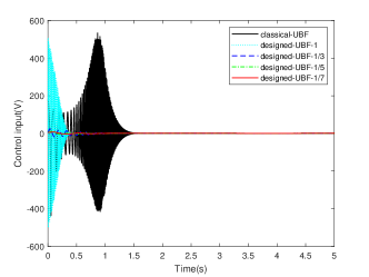
(a) Control inputs with classical and designed UBF

(b) Control inputs with designed UBF

Figure 2: Control inputs

The numerical simulation results are plotted in Fig. 2 (a)-(b). It is observed that by selecting appropriate designed parameters, the newly developed UBF can effectively diminish the consumption of the control input energy caused by the introduction of constraints.

IV-B The simulation of attitude tracking control

In this study, the PF parameters are designed as: ${T_{s}}=1.2,\Delta=0.05,{e_{\infty}}=0.01$, and the parameters of the designed UBF are selected as: ${c_{1}}={c_{2}}=0.2,m=n=\frac{1}{7}$, while the other parameters are identical to those in simulation I. The developed control protocol without PF, and the CFB algorithm in [2] without RBFNN are adopted as the contrasting approaches.

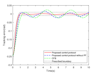
Figure 3: Tracking errors

The curves of the tracking error are displayed in Fig. 3, which demonstrates that the attitude tracking error can converge to a predefined region within a designer-defined time. Furthermore, the tracking error owns better transient behavior, especially small overshoot.

V Conclusion

A novel prescribed performance adaptive fixed-time backstepping control protocol was proposed in this article to tackle the attitude tracking problem of a 3-DOF helicopter subject to disturbances. A newly designed UBF was adopted to transform the prescribed performance constrained system into an unconstrained one. By virtual of an improved FxT backstepping control algorithm, the attitude tracking was fulfilled. A modified FxT stability theorem was presented to provide a less conservative and more accurate approximation of the settling time than the classical result. Theoretical analysis proves that all signals of the system are FxT bounded, while the tracking error converges to a predetermined domain with small overshoot in a user-defined time. Simulation results show the feasibility and effectiveness of the presented control strategy.

References

• [1] Z. Li, H. H. T. Liu, B. Zhu, H. Gao, and O. Kaynak, “Nonlinear robust attitude tracking control of a table-mount experimental helicopter using output feedback,” IEEE Transactions on Industrial Electronics, vol. 62, no. 9, pp. 5665–5676, 2015.
• [2] C. Li and X. Yang, “Neural networks-based command filtering control for a table-mount experimental helicopter,” Journal of the Franklin Institute, vol. 358, no. 1, pp. 321–338, 2021.
• [3] J. Yu, P. Shi, and L. Zhao, “Finite-time command filtered backstepping control for a class of nonlinear systems,” Automatica, vol. 92, pp. 173–180, 2018.
• [4] A. Loza, H. Ríos, and A. Rosales, “Robust regulation for a 3-DOF helicopter via sliding-mode observation and identification,” Journal of the Franklin Institute, vol. 349, no. 2, pp. 700–718, 2012.
• [5] F. Plestan and A. Chriette, “A robust controller based on adaptive super-twisting algorithm for a 3DOF helicopter,” in 2012 IEEE 51st IEEE Conference on Decision and Control (CDC), pp. 7095–7100, 2012.
• [6] H. Castañeda, F. Plestan, A. Chriette, and J. de León-Morales, “Continuous differentiator based on adaptive second-order sliding-mode control for a 3-DOF helicopter,” IEEE Transactions on Industrial Electronics, vol. 63, no. 9, pp. 5786–5793, 2016.
• [7] X. Wang, Z. Li, Z. He, and H. Gao, “Adaptive fast smooth second-order sliding mode control for attitude tracking of a 3-DOF helicopter,” arXiv e-prints, p. arXiv:2008.10817, Aug. 2020.
• [8] X. Wang, “Adaptive smooth disturbance observer-based fast finite-time adaptive backstepping control for attitude tracking of a 3-DOF helicopter,” arXiv e-prints, p. arXiv:2106.13940, Jun. 2021.
• [9] A. Polyakov, “Nonlinear feedback design for fixed-time stabilization of linear control systems,” IEEE Transactions on Automatic Control, vol. 57, no. 8, pp. 2106–2110, 2012.
• [10] J. Ni and P. Shi, “Adaptive neural network fixed-time leader-follower consensus for multiagent systems with constraints and disturbances,” IEEE Transactions on Cybernetics, vol. 51, no. 4, pp. 1835–1848, 2021.
• [11] H. Wang, K. Xu, and J. Qiu, “Event-triggered adaptive fuzzy fixed-time tracking control for a class of nonstrict-feedback nonlinear systems,” IEEE Transactions on Circuits and Systems I: Regular Papers, vol. 68, no. 7, pp. 3058–3068, 2021.
• [12] J. Ni, P. Shi, Y. Zhao, and Z. Wu, “Fixed-time output consensus tracking for high-order multi-agent systems with directed network topology and packet dropout,” IEEE/CAA Journal of Automatica Sinica, vol. 8, no. 4, pp. 817–836, 2021.
• [13] K. Li, Y. Li, and G. Zong, “Adaptive fuzzy fixed-time decentralized control for stochastic nonlinear systems,” IEEE Transactions on Fuzzy Systems, vol. 29, no. 11, pp. 3428–3440, 2021.
• [14] C. P. Bechlioulis and G. A. Rovithakis, “Robust adaptive control of feedback linearizable mimo nonlinear systems with prescribed performance,” IEEE Transactions on Automatic Control, vol. 53, no. 9, pp. 2090–2099, 2008.
• [15] Y. Liu, X. Liu, Y. Jing, and Z. Zhang, “A novel finite-time adaptive fuzzy tracking control scheme for nonstrict feedback systems,” IEEE Transactions on Fuzzy Systems, vol. 27, no. 4, pp. 646–658, 2019.
• [16] J. Ni, C. K. Ahn, L. Liu, and C. Liu, “Prescribed performance fixed-time recurrent neural network control for uncertain nonlinear systems,” Neurocomputing, vol. 363, no. 21, pp. 351–365, 2019.
• [17] G. Cui, W. Yang, J. Yu, Z. Li, and C. Tao, “Fixed-time prescribed performance adaptive trajectory tracking control for a QUAV,” IEEE Transactions on Circuits and Systems II: Express Briefs, pp. 1–1, 2021.
• [18] R. Aldana-López, D. Gómez-Gutiérrez, E. Jiménez-Rodríguez, J. D. Sánchez-Torres, and M. Defoort, “Enhancing the settling time estimation of a class of fixed-time stable systems,” International Journal of Robust and Nonlinear Control, vol. 29, no. 12, 2019.
• [19] Z. Zheng, M. Feroskhan, and L. Sun, “Adaptive fixed-time trajectory tracking control of a stratospheric airship,” ISA transactions, vol. 76, pp. 134–144, 2018.
• [20] Z. Guan, H. Liu, Z. Zheng, M. Lungu, and Y. Ma, “Fixed-time control for automatic carrier landing with disturbance,” Aerospace Science and Technology, vol. 108, p. 106403, 2021.
• [21] S. Parsegov, A. Polyakov, and P. Shcherbakov, “Nonlinear fixed-time control protocol for uniform allocation of agents on a segment,” in 2012 IEEE 51st IEEE conference on decision and control (CDC), pp. 7732–7737, 2012.
• [22] P. Sun, B. Zhu, Z. Zuo, and M. V. Basin, “Vision-based finite-time uncooperative target tracking for UAV subject to actuator saturation,” Automatica, vol. 130, p. 109708, 2021.
• [23] C. Qian and W. Lin, “A continuous feedback approach to global strong stabilization of nonlinear systems,” IEEE Transactions on Automatic Control, vol. 46, no. 7, pp. 1061–1079, 2001.
• [24] X. Huang, W. Lin, and B. Yang, “Global finite-time stabilization of a class of uncertain nonlinear systems,” Automatica, vol. 41, no. 5, pp. 881–888, 2005.
• [25] X. Wang, “Smooth attitude tracking control of a 3-dof helicopter with guaranteed performance,” arXiv e-prints, p. arXiv:2101.11241, Jan. 2021.
• [26] E. Cruz Zavala, J. A. Moreno, and L. M. Fridman, “Uniform robust exact differentiator,” IEEE Transactions on Automatic Control, vol. 56, no. 11, pp. 2727–2733, 2011.
• [27] K. Zhao, Y. Song, C. P. Chen, and L. Chen, “Control of nonlinear systems under dynamic constraints: A unified barrier function-based approach,” Automatica, vol. 119, p. 109102, 2020.