Physics-Aware Safety-Assured Design of
Hierarchical Neural Network based Planner

Abstract.

Neural networks have shown great promises in planning, control, and general decision making for learning-enabled cyber-physical systems (LE-CPSs), especially in improving performance under complex scenarios. However, it is very challenging to formally analyze the behavior of neural network based planners for ensuring system safety, which significantly impedes their applications in safety-critical domains such as autonomous driving. In this work, we propose a hierarchical neural network based planner that analyzes the underlying physical scenarios of the system and learns a system-level behavior planning scheme with multiple scenario-specific motion-planning strategies. We then develop an efficient verification method that incorporates overapproximation of the system state reachable set and novel partition and union techniques for formally ensuring system safety under our physics-aware planner. With theoretical analysis, we show that considering the different physical scenarios and building a hierarchical planner based on such analysis may improve system safety and verifiability. We also empirically demonstrate the effectiveness of our approach and its advantage over other baselines in practical case studies of unprotected left turn and highway merging, two common challenging safety-critical tasks in autonomous driving.

1. Introduction

Neural network based machine learning techniques have been increasingly leveraged in learning-enabled cyber-physical systems (LE-CPSs) (Tuncali et al., 2018; Wang et al., 2020a) for perception, prediction, planning, control, etc. In particular, neural networks may greatly improve performance and efficiency for planning and general decision making in LE-CPSs, such as autonomous driving (Ha et al., 2020), human robot interaction (Fisac et al., 2018), smart grid (Lu and Hong, 2019) and smart buildings (Wei et al., 2017). Moreover, compared with traditional model-based approaches, they can save the time and effort of explicitly modeling systems with complex dynamics and significant uncertainties. However, a major challenge for the neural network based planners is to ensure system safety, especially for safety-critical applications (Zhu et al., 2021) and in near-accident scenarios (Fan et al., 2020; Cao et al., 2020a), such as unprotected left turn and highway merging in autonomous driving. In those scenarios, with only minor changes in environment states, dramatically different behaviors may need to be performed to avoid accidents, which is difficult for both humans and autonomous systems to handle. Our work focuses on addressing such complex scenarios in safety-critical systems.

In this work, we first observe that for systems that may evolve into different physical scenarios under a single neural network based planner, it is often difficult to verify their safety or the planner is indeed unsafe. And we conduct theoretical analysis to show the reason. Based on such observation and the fact that many safety-critical systems may evolve into multiple different physical scenarios and thus require dramatically different behaviors to ensure their safety and improve efficiency, we propose a hierarchical neural network based planner that consists of a system-level behavior planner and multiple scenario-specific motion planners. We then develop an efficient verification method that incorporates novel partition and union techniques and an approach for overapproximating system state reachable set to formally verify the system safety under our hierarchical planner. More specifically, our planner design and verification method address the key open challenges in ensuring the safety of neural network based planners, as follows.

Hierarchical Planner Design: We propose a hierarchical planner design for safety-critical systems to improve both system safety and verifiability. Recently, a variety of neural network based planner designs, including hierarchical planners, have been developed for various applications due to their strengths in improving system performance and reducing accident rate in average (Stock et al., 2015; Cao et al., 2020a; Pettet et al., 2020). However, it is very challenging to formally provide safety guarantee in the worst case for those systems. In particular, we consider the safety-critical systems that may evolve into different physical scenarios based on the dynamic situation, which under a well-designed planner should lead into multiple disjoint subsets of the system state reachable set. We leverage the concept of Lipschitz constant in our theoretical analysis and show that for such systems, most single neural network based planners are either unsafe or will result in significantly harder verification problems when the Lipschitz constant goes to infinity. This motivates our design of a hierarchical planner, which consists of a system-level behavior planner and multiple low-level motion planners, each of which corresponds to an underlying physical scenario for the system. As shown later, our hierarchical planner design, combined with the corresponding improvement in the verification tool, enables formal verification and assurance of system safety.

Efficient Verification: Our design of the hierarchical neural network based planner brings significant challenges but also opportunities for system safety verification. In particular, reachability analysis is a popular formal technique for verifying system safety, with various recent methods for LE-CPSs (Tran et al., 2019; Huang et al., 2019; Dutta et al., 2019; Ivanov et al., 2019). However, these methods cannot be directly applied to systems under our hierarchical planner, and have limited efficiency and accuracy for safety-critical systems that are sensitive to environment changes. To address these challenges, we first develop new partition and union techniques to overcome the limitations in efficiency and accuracy, and then develop a verification method based on the overapproximated reachable set of both behavior planner and selected motion planners for ensuring system safety.

Related Work: Our work is related to a rich literature of planner design and system safety verification. There are a number of varied planner designs, including classical rule-based (Farag, 2019), optimization-based (Liu et al., 2020b) and game theory-based (Liu et al., 2020a) planners, as well as emerging neural network based planners. Many recent neural network based planners demonstrate significant performance improvement and accident rate reduction in average over traditional model-based methods. Some of those learn a single neural network for planning via reinforcement learning (Cao et al., 2020b), imitation learning (Chen et al., 2019), supervised learning (Markolf et al., 2020), etc., while others employ a hierarchical planner design (Zheng et al., 2017; Cao et al., 2020a), which usually consists of low-level planners for different modes and a high-level planner that is responsible for selecting the mode. However, even though safety improvement is often considered and demonstrated empirically through experiments in those works (Naveed et al., 2020; Cao et al., 2020a; Nosrati et al., 2018; Li et al., 2021; Wang et al., 2020b; Ma et al., 2021), formal system safety verification remains a challenging problem. In contrast, our work focuses on formal safety verification, with a hierarchical neural network based planner design that considers the different underlying physical scenarios a system may evolve into.

In terms of safety verification techniques, most recent works present results in ensuring safety for relatively simple scenarios, such as adaptive cruise control and emergency braking (Tran et al., 2019; Huang et al., 2020). Different from these works, we focus on safety verification for complex systems that may evolve into multiple different physical scenarios and thus have multiple disjoint reachable set. Our approach verifies systems by computing a bounded time reachable set. However, different from the verification of neural network controlled systems in the literature (Huang et al., 2019; Fan et al., 2019; Ivanov et al., 2019; Dutta et al., 2019; Tran et al., 2020), where a single planner is considered, our work addresses a hierarchical planner and thus considers a hybrid system. Specifically, we develop novel partition and union techniques across reachability analysis to improve efficiency and accuracy.

In summary, our work makes the following contributions:

• With empirical study and theoretical analysis, we show that for those systems that may evolve into multiple physical scenarios, single neural network based planner is either unsafe, or extremely difficult to verify.

• We design a novel hierarchical neural network based planner with assured safety and better verifiability, based on the underlying physical scenarios of the system.

• We develop novel partition and union techniques to improve efficiency and accuracy of reachability analysis, and propose an overapproximation method for the system under our hierarchical planner.

• We demonstrate the safety enhancement from our hierarchical design through case studies of unprotected left turn and highway merging, compared with single neural network based planners.

The rest of the paper is organized as follows. Section 2 introduces an illustrating example and defines the problem formulation. Section 3 presents our planner design and verification approach. Section 4 shows the case studies and Section 5 concludes the paper.

2. Problem Formulation

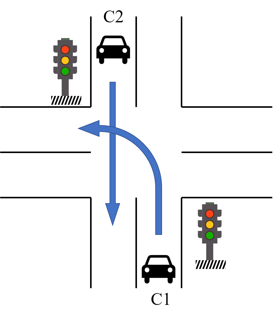
Figure 1. The unprotected left turn system.

We consider the unprotected left turn as a representative application where different planning decisions and system states can eventually lead to different physical scenarios. The system includes a left turn vehicle $C1$ and another vehicle $C2$ going straight from the opposite direction in an intersection, as shown in Fig. 1. We model it as a 5-dimensional system:

(1) $$\begin{cases}\dot{p}_{1}(t)=v_{1}(t)\\ \dot{v}_{1}(t)=u(t)\\ \dot{\tau}_{min}(t)=f_{1}(t)\\ \dot{\tau}_{max}(t)=f_{2}(t)\\ \dot{t}=1\end{cases}$$

where $p_{1}(t)$ and $v_{1}(t)$ are the position and velocity of vehicle $C1$. Vehicle $C2$ is predicted to pass the conflicting area (where the two vehicles may potentially collide) in this intersection within the time window $\left[\tau_{min}(t)\text{, }\tau_{max}(t)\right]$. $u(t)$ is the control input, representing the acceleration of vehicle $C1$. We assume that vehicle $C1$ follows a given path in the intersection to turn left, thus its trajectory can be derived with $u(t)$. $\tau_{min}(t)$ and $\tau_{max}(t)$ may change over time as vehicle $C1$ can update its prediction for $C2$. We assume that this time window will become tighter as two vehicles get closer to each other, i.e., $f_{1}(t)>=0$ and $f_{2}(t)<=0$. We also assume that the traffic signal follows a fixed pattern. First it is green for $t_{g}$ seconds, then it turns yellow for $t_{y}$ seconds, and then it turns red for $t_{r}$ seconds. After that, it turns back to green and repeats this turning pattern.

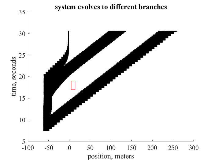
Figure 2. System in Fig. 1 evolves to multiple physical scenarios. The horizontal axis denotes the position of vehicle $C1$ along the planned path, and a negative value means that $C1$ has not entered the intersection. The vertical axis denotes time. The black region represents simulated trajectories of the system. From left to right, the three branches correspond to the scenarios where vehicle $C1$ stops before the intersection, yields to $C2$, and proceeds, respectively. The red rectangle is the unsafe region as vehicle $C2$ is expected to passing the intersection at time interval $\left[17\text{, }19\right]$.

Fig. 2 shows the simulated trajectories based on human driving norm. The horizontal axis denotes the position of vehicle $C1$ along the planned path, where a negative value represents that $C1$ has not entered the intersection. When $p_{1}=4.5$ meters, $C1$ enters the region where two vehicles’ paths may intersect. When $p_{1}=14$ meters, it leaves that conflicting region. There are three obvious branches as time goes on. The leftmost branch corresponds to the behavior of $C1$ stopping before the intersection, when it cannot pass the intersection before the signal turns red. The middle branch corresponds to the behavior of $C1$ yielding to vehicle $C2$ that goes straight, when there is potential danger for collision and $C2$ has the right of way. The rightmost branch corresponds to the behavior of $C1$ proceeding, when it is safe to pass the intersection before $C2$. The red rectangle marks the unsafe region, as vehicle $C2$ is expected to pass the conflicting region within the time window $\left[\tau_{min}(t)\text{, }\tau_{max}(t)\right]\equiv\left[17\text{, }19\right]$ seconds.

To react safely and efficiently, depending on the initial system state and changes in the surrounding traffic, vehicle $C1$ may take different actions. Note that although there may exist some planner $u^{\prime}(t)$ that is safe and can lead to only one branch of system trajectories, i.e., braking and then stopping before the intersection in any case, it is not efficient and ideal in real life.

In some simpler systems such as adaptive cruise control and emergency braking (Tran et al., 2019; Huang et al., 2020), the system state may converge to a constant distance gap or gradually slows down to full stop. Here, the potential reachable states of the unprotected left turn system do not converge to a single scenario, but evolve to multiple different scenarios. This presents significant challenges to safety verification and assurance.

Thus, in this work, we are interested in the following questions: Can vehicle $C1$ turn left safely and efficiently under our designed planner when facing different traffic scenarios, i.e., turning left without hesitance when it is safe and decelerating when facing potential collision? If so, can we formally verify the system safety under our designed planner? To answer these, we will first generally formulate the above-mentioned system where different planning decisions and system states can eventually lead to different physical scenarios.

General Formulation. We consider a dynamic system:

(2) $$\begin{cases}\dot{x}(t)=f(x(t)\text{, }u(t))\text{, }\forall t\geq 0\\ x(t)\in X-S_{u}\text{, }x(0)\in I\text{, }u(t)\in U\end{cases}$$

where $x(t)$ is the state variable, and $u(t)$ is the control input variable. We assume that $f$ is Lipschitz continuous in $x$ and continuous in $u$ to ensure the uniqueness of solution. By including time $t$ in state variable $x(t)$, system function $f$ can be time-variant. $X=\{x\in{\mathbb{R}}^{n}\}$ is the state space. $S_{u}=\{x\in{\mathbb{R}}^{n}|\underset{i}{\land}h_{i}(x)\leq 0\}$ is the unsafe state space, $h$ denotes the linear constraint function and state $x$ is unsafe if $\underset{i}{\land}h_{i}(x)\leq 0$ is satisfied. $X-S_{u}$ is the set difference of $X$ and $S_{u}$. $I\subseteq X-S_{u}$ is the initial set of system state. $U=\{u\in{\mathbb{R}}^{m}\}$ is the control input space.

Let $\delta_{c}$ denote the control time stepsize. At time $t=i*\delta_{c}$, $i=0\text{, }1\text{, }2\text{, \ldots}$, the system controller $\kappa$ takes current state $x(i*\delta_{c})$ and computes control input $u(i*\delta_{c})=\kappa(x(i*\delta_{c}))$ for the next time step, the system becomes $\dot{x}(t)=f(x(t)\text{, }u(i*\delta_{c}))$ in the time interval $t\in\left[i*\delta_{c}\text{, }(i+1)*\delta_{c}\right]$.

The trajectory $\varphi_{x(0)}$ to the system (2) starting from an initial state $x(0)$ can be formulated as:

(3) $$\dot{\varphi}_{x(0)}(t)=f(\varphi_{x(0)}(t)\text{, }u(t))\text{, }x(0)\in I$$

where $\varphi_{x(0)}(0)=x(0)$.

With a well-designed controller $u(t)$, the system trajectories will evolve to disjoint subsets at step $i$ (and possibly at the following steps as well) to avoid the unsafe set. That is:

(4) $$\begin{cases}\varphi_{x(0)}(t)\in\underset{k}{\cup}S_{k}\text{, }\forall t\in\left[(i-1)*\delta_{c}\text{, }i*\delta_{c}\right]\text{, }\forall x(0)\in I\\ ||x-x^{\prime}||>\epsilon_{x}\text{, }\exists\epsilon_{x}>0\text{, }\forall x\in S_{k}\text{, }\forall x^{\prime}\in S_{j}\text{, }\forall k\neq j\end{cases}$$

where $\delta_{c}$ is the control time stepsize, $S_{k}$ is a subset of system states in time interval $\left[(i-1)*\delta_{c}\text{, }i*\delta_{c}\right]$, $\underset{k}{\cup}S_{k}$ is the union of all subsets. The distance between any two elements $x\in S_{k}$ and $x^{\prime}\in S_{j}$ is always strictly greater than a positive real number $\epsilon_{x}$, for any two different subsets $S_{k}$ and $S_{j}$.

It becomes more challenging to design a safety-assured planner due to the properties of the system as in (2) and (4). Since the safe state space $X-S_{u}$ is non-convex, the system reachable set needs to evolve to multiple branches to avoid the unsafe set. However, a planner $\kappa(x)$ that is Lipschitz continuous in $x$ intuitively cannot output significant different control signal $u(x)$ under only minor changes in system state $x$. For these complex systems, accidents cannot be prevented in experiments with previous neural network based planner designs, including hierarchical planners (Naveed et al., 2020; Cao et al., 2020a; Nosrati et al., 2018; Li et al., 2021; Wang et al., 2020b; Ma et al., 2021). Thus, we try to answer: is there a planner design that can enable the change of system trajectory under changing scenarios? If so, can we verify its safety as the system reachable states evolve to multiple possible scenarios? Formally, we try to solve:

Problem 1.

For a dynamical system defined by (2) and (3), is there a planner design $\kappa$ that can satisfy (4)?

Problem 2.

If there exists a planner $\kappa$ that can satisfy (4), the safety verification problem is to determine whether the controlled trajectory $\varphi_{x(0)}(t)\in X-S_{u}\text{, }\forall t\geq 0\text{, }\forall x(0)\in I$.

3. Planner Design and Safety Verification

In this section we first conduct formal analysis for systems under a single neural network based planner. With theoretical analysis, we show that single neural network planners cannot handle well the systems that may evolve into different scenarios, and are hard to verify. To overcome these challenges, we present our design of a hierarchical neural network based planner, and then introduce the partition and union algorithm we developed for the verification of our hierarchical planner.

3.1. Formal Analysis of Single Planner Design

Using a single neural network for planner design is well-studied (Chen et al., 2020; Qureshi et al., 2020; Seidman et al., 2020). Deep neural networks provide better performance for complex systems than many traditional methods (Dong et al., 2020; Zhou et al., 2019; Zeng et al., 2019). However, single neural network based planner has its limitations, especially for safety-critical systems (Cao et al., 2020a). Below we formally analyze the system under a single neural network based planner with reachability analysis of a neural network controlled system (Tran et al., 2020; Huang et al., 2019; Ivanov et al., 2019; Dutta et al., 2019), and we leverage the Bernstein polynomial based reachability analysis (Huang et al., 2019), as it can handle neural networks with general and heterogeneous activation functions. Let us start with introducing reachable set and Bernstein polynomial.

Definition 3.0.

A system state $x$ is reachable at time $t\geq 0$ on a system defined by (2) and (3), if and only if there exists $x(0)\in I$ such that $x=\varphi_{x(0)}(t)$. The reachable set $R$ of the system is defined as the set of all reachable states $R=\{x|x=\varphi_{x(0)}(t)\text{, }\forall t\geq 0\text{, }\forall x(0)\in I\}$.

The system is considered to be safe if its reachable set $R$ has no overlap with the unsafe set $S_{u}$. However, it is proven that computing the exact reachable set for most nonlinear systems is an undecidable problem (Henzinger et al., 1998), not to mention systems with neural network planners. Thus, recent works mainly consider overapproximation of the reachable set. Safety can still be guaranteed if the overapproximated reachable set has no overlap with the unsafe set. Note that in this paper, for simplificy, we use the same notation for both the reachable set and its overapproximation.

For a controller/planner $\kappa_{s}$ defined over a n-dimensional state $x$, its Bernstein polynomials $B_{\kappa_{s},d}(x)$ under degree $d=(d_{1}\text{, }d_{2}\text{, \ldots, }d_{n})$ is:

(5) $$B_{\kappa_{s},d}(x)= \sum_{\begin{subarray}{c}0\leq a_{j}\leq d_{j}\\ j\in\{1\text{, }2\text{, \ldots, }n\}\end{subarray}}\kappa_{s}\bigg{(}\frac{a_{1}}{d_{1}}\text{, }\frac{a_{2}}{d_{2}}\text{, \ldots, }\frac{a_{n}}{d_{n}}\bigg{)}$$

$$\prod_{j=1}^{n}\bigg{(}\Big{(}\begin{subarray}{c}d_{j}\\ a_{j}\end{subarray}\Big{)}x^{a_{j}}_{j}(1-x_{j})^{d_{j}-a_{j}}\bigg{)}$$

where $\Big{(}\begin{subarray}{c}d_{j}\\ a_{j}\end{subarray}\Big{)}$ is a binomial coefficient.

To obtain an overapproximation of the reachable set for a system with a neural network based controller $\kappa_{s}$, we compute an overapproximation of the controller $\kappa_{s}$ using Bernstein polynomials similarly as in (Huang et al., 2019). Note that the reachable set is computed step by step and it is sufficient to perform the overapproximation of $\kappa_{s}$ at step $i$ on the latest computed reachable set $R_{i-1}$. That is, $\kappa_{s}$ is overly approximated by a Bernstein polynomial with bounded error $\epsilon$ on set $R_{i-1}$ as:

(6) $$\kappa_{s}(x)\in B_{\kappa_{s},d}(x)+\left[-\epsilon\text{, }\epsilon\right]\text{, }\forall x\in R_{i-1}$$

where $R_{0}=I$ when performing overapproximation in the first step. In the rest of the paper, $B_{\kappa_{s}}(x)$ is short for $B_{\kappa_{s},d}(x)$, as it is not necessary to have the same $d$ for the overapproximation of different controllers.

With the above approach, the dynamic system with a single neural network based planner $\kappa_{s}$ is transformed into a polynomial system for computing the overapproximation of the reachable set. This enables our following analysis.

Challenge on correctness. Intuitively it is unlikely that Lipschitz continuous planners can output significantly different control signal $u(x)$ under only minor changes in the system state $x$, and enable system trajectory go into several disjoint subsets under different scenarios. Next, let us formally introduce Lipschitz constant and explain that a large number of single neural network planners may indeed be unsafe for the system.

Definition 3.0.

A real-valued function $f:X\rightarrow\mathbb{R}$ is called Lipschitz continuous over $X\subseteq\mathbb{R}^{n}$, if there exists a non-negative real $L$, such that $||f(x)-f(x^{\prime})||\leq L||x-x^{\prime}||$ for $\forall x$, $x^{\prime}\in X$. Any such $L$ is called a Lipschitz constant of $f$ over $X$.

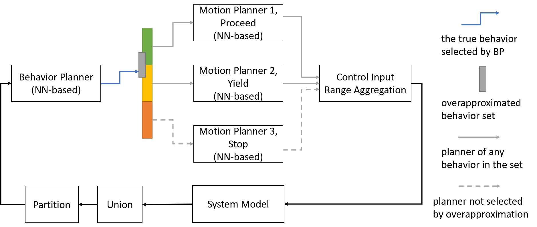
Figure 3. Our design of the hierarchical neural network based planner consists of one behavior planner $\mu$ and $N$ motion planners $\{\kappa_{1}\text{, }\kappa_{2}\text{, \ldots, }\kappa_{N}\}$. Take the unprotected left turn system as an example, there are three underlying physical scenarios: vehicle $C1$ may stop before the intersection, yield to vehicle $C2$, or proceed, and they correspond to three motion planners shown here in the figure. The behavior planner decides the most appropriate behavior for vehicle $C1$ given the system state $x$, and then the corresponding motion planner is enabled to control the system. To compute an overapproximation of the reachable set of the system under such hierarchical planner, we first compute an overapproximated behavior set with Bernstein polynomial approximation as in Eq. (5) and (6), which is illustrated by the grey rectangle in the figure. Then for each behavior in the overapproximated behavior set, the corresponding motion planner’s output range can be aggregated as the possible control input range, thus computing an overapproximation of the system state reachable set under all possible behaviors.

Proposition 3.3.

For a dynamical system defined by (2) and (3) with single neural network based planner $\kappa_{s}$, if $\kappa_{s}$ is a convolutional or fully connected neural network with ReLU, sigmoid or hyperbolic tangent (tanh) activation functions, then the controlled trajectory $\varphi_{x^{\prime}(0)}(t^{\prime})$ will not evolve to several branches as formulated in (4).

Proof.

We will first prove that if a neural network planner $\kappa_{s}$ can ensure that the system evolves to several branches as defined in (4), $\kappa_{s}$ is not Lipschitz continuous. We assume it is at step $i$ that the reachable set $R_{i}$ can be represented as $R_{i}=\underset{k}{\cup}S_{k}$ as in (4) for the first time. Then there exists $x_{i-1}\in R_{i-1}$ and $x^{\prime}_{i-1}\in R_{i-1}$ such that $||x_{i-1}-x^{\prime}_{i-1}||\rightarrow 0$, $x_{i-1}+f(x_{i-1}\text{, }\kappa_{s}(x_{i-1}))*\delta t=x_{i}\in R_{k}$, $x^{\prime}_{i-1}+f(x^{\prime}_{i-1}\text{, }\kappa_{s}(x^{\prime}_{i-1}))*\delta t=x^{\prime}_{i}\in R_{j}$, $k\neq j$ and $\delta t\rightarrow 0$. According to (4), there exists $\epsilon_{x}>0$ such that $||x_{i}-x^{\prime}_{i}||>\epsilon_{x}$, and we have $||f(x_{i-1}\text{, }\kappa_{s}(x_{i-1}))-f(x^{\prime}_{i-1}\text{, }\kappa_{s}(x^{\prime}_{i-1}))||>\epsilon_{f}$ and $\epsilon_{f}>0$. Because $f$ is Lipschitz continuous, then $\kappa_{s}$ is not Lipschitz continuous. However, since $\kappa_{s}$ is a convolutional or fully connected neural network with ReLU, sigmoid and hyperbolic tangent (tanh) activation functions, it should be Lipschitz continuous (Huang et al., 2019). From this contradiction, we know that the controlled trajectory $\varphi_{x^{\prime}(0)}(t^{\prime})$ will not evolve to several branches as formulated in (4). ∎

Based on this proposition, for most single neural network based planners, the system reachable set will cover the unsafe region $S_{u}$ and there is actually no disjoint subsets.

Challenge on verifiability. Even if $\kappa_{s}$ is a neural network based planner that can satisfy (4), it will have infinitely large Lipschitz constant according to Proposition 3.3. This typically makes the safety verification extremely hard due to the importance of Lipschitz constant in the construction of reachable sets. As observed in (Fan et al., 2019; Wang et al., 2021; Ivanov et al., 2019) and shown in our case studies in Sections 4.1.1 and 4.2.1, the reachable set expands more quickly when the Lipschitz constant of neural network based planner is larger. In which case, the verification process may terminate due to uncontrollable approximation error or excessively long computation time. These challenges can be overcome in our hierarchical planner design as introduced below.

3.2. Hierarchical Planner Design and Reachability Analysis

Hierarchical planner design. The drawbacks of a single neural network based planner motivates us to propose a hierarchical planner, as shown in Fig. 3. The main idea is to learn different motion planners for different physical scenarios and a system-level behavior planner for changing between scenarios. Specifically, our hierarchical planner consists of a behavior planner $\mu$ and $N$ motion planners $\{\kappa_{1}\text{, }\kappa_{2}\text{, \ldots, }\kappa_{N}\}$, assuming that the system may evolve into $N$ different physical scenarios. These planners are all neural network based and take system states as inputs. The behavior planner’s output $\mu(x)$ can be mapped to the discrete behavior choice by mapping function $f_{m}$ and we have $f_{m}(\mu(x))\in\{\kappa_{1}\text{, }\kappa_{2}\text{, \ldots, }\kappa_{N}\}$, while motion planners output control variable $u(t)$. To illustrate the idea, we still use the unprotected left turn system as an example: The behavior planner will decide the most appropriate behavior for vehicle $C1$ given the system state $x$. Then the corresponding motion planner, e.g., motion planner $2$ in Fig. 3, will be enabled to control the system. The system will use the same motion planner before the next triggering of the behavior planner. Note that it is flexible to set the trigger conditions for the behavior planner, e.g., behavior planner may be triggered every $t_{bp}$ seconds when the system state has significant changes.

The challenges under a single neural network planner $\kappa_{s}$ can be overcome in our hierarchical planner design as the reachable sets computed under different motion planners correspond to different physical scenarios and are disjoint. For each underlying physical scenario, the corresponding motion planner can generate system trajectory to avoid the unsafe region. Given that all motion planners are safe in their corresponding scenarios, system safety can be guaranteed with the computation of an overapproximated behavior set for the system-level behavior planner.

Reachability verification. Next we first present our partition and union algorithm for general reachable set computation to improve efficiency and accuracy, and then we introduce our method to overapproximate the reachable set for a system under a hierarchical planner $\mu(\kappa_{1}\text{, }\kappa_{2}\text{, \ldots, }\kappa_{N})$.

Result: Reachable set $R$ and verification result

Input : Initial set $I$, unsafe set $S_{u}$ and goal set $S_{g}$

1 $R\leftarrow I$;

2 while $I-S_{g}\neq\emptyset$ and $R\cap S_{u}=\emptyset$ do

3       $\{I_{\gamma}\}\leftarrow Partition(I\text{, }\delta)$;

4       for each grid $I_{\gamma}$ do

5             $R_{\gamma}\leftarrow Reach\_Comp(I_{\gamma}\text{, }n)$;

6             while $Reach\_Comp$ terminates without returning $R_{\gamma}$ do

7                   $\{I_{\gamma^{\prime}}\}\leftarrow Partition(I_{\gamma}\text{, }\delta/2)$;

8                   for each grid $I_{\gamma^{\prime}}$ do

9                         $R_{\gamma^{\prime}}\leftarrow Reach\_Comp(I_{\gamma^{\prime}}\text{, }n)$;

10                        

11                   end for

12                  

13             end while

14            

15       end for

16      $I\leftarrow\underset{\gamma}{\cup}R_{\gamma}$;

17       $R\leftarrow R\cup I$;

18      

19 end while

20if $R\cap S_{u}=\emptyset$ then

21       Verification result is safe. 

22else

23       Verification result is uncertain. 

24 end if

Algorithm 1 Partition and Union for Reachable Set Computation

We develop a partition and union method that can improve the efficiency and accuracy of the overapproximated reachable set at every computation step, as shown in Algorithm 1. Specifically, when the system state has not fully reached the goal set $S_{g}$ and the system is currently safe (line 2), we will keep computing the reachable set as follows. We first partition the initial set $I$ into grids of size $\delta$ (line 3), and then compute the reachable set for each grid $I_{\gamma}$ in the next $n$ steps (line 5). The computation process may terminate without returning $R_{\gamma}$ (line 6) due to memory limitation, low accuracy or no result within certain time. In that case, we will further partition the initial set $I_{\gamma}$ (line 7) and compute the reachable set (line 9). Once the reachable set $R_{\gamma}$ is computed for each grid, we union them as the system reachable set for this round, and reset the initial set $I=\underset{\gamma}{\cup}R_{\gamma}$ (line 13). This process repeats until the system state reaches the goal set $S_{g}$ and is verified to be safe, or the overapproximation of the reachable set has overlap with the unsafe set $S_{u}$ (which presents an uncertain verification results given the nature of overapproximation).

To compute an overapproximated reachable set for a system with planner $\mu(\kappa_{1}\text{, }\kappa_{2}\text{, \ldots, }\kappa_{N})$, we first overapproximate $\mu(x)$ in a similar way as in (6) as:

(7) $$\mu(x)\in B_{\mu}(x)+\left[-\epsilon_{\mu}\text{, }\epsilon_{\mu}\right]\text{, }\forall x\in R_{i-1}$$

where $R_{i-1}$ is the overapproximated reachable set of the system in the $(i-1)$-th step. We then compute the overapproximated output range of $\mu(x)$, $R_{i}^{\mu}$, on the set $R_{i-1}$. By the mapping function $f_{m}$, we have the overapproximated set of the selected planner $S_{ctrl}\subseteq\{\kappa_{1}\text{, }\kappa_{2}\text{, \ldots, }\kappa_{N}\}$. For any planner $\kappa_{a}(x)\in S_{ctrl}$, we can compute its overapproximated system state reachable set $R^{\kappa_{a}}_{i}$ on $R_{i-1}$. Then, the overapproximated reachable set of the system at step $i$ is $R_{i}=\underset{\kappa_{a}\in S_{ctrl}}{\cup}R^{\kappa_{a}}_{i}$. The soundness of our approach can be proven below.

Proposition 3.4.

(Soundness). For a dynamical system defined by (2), (3) and (4) with a hierarchical neural network based planner $\mu(\kappa_{1}\text{, }\kappa_{2}\text{, \ldots, }\kappa_{N})$, the controlled trajectory $\varphi_{x(0)}(t)$ satisfies $\varphi_{x(0)}(t)\in\underset{\kappa_{a}\in S_{ctrl}}{\cup}R^{\kappa_{a}}_{i}\text{, }\forall t\in\left[(i-1)*\delta_{c}\text{, }i*\delta_{c}\right]\text{, }\forall i\in\mathbb{N}^{+}\text{, }\forall x(0)\in I$.

Proof.

Let us prove by contradiction. We assume that it is at step $i$ that we compute the wrong reachable set $R_{i}=\underset{\kappa_{a}\in S_{ctrl}}{\cup}R^{\kappa_{a}}_{i}$ for the first time. Thus $\exists x^{\prime}(0)\in I$ and $\exists\kappa^{\prime}\in\{\kappa_{1}\text{, }\kappa_{2}\text{, \ldots, }\kappa_{N}\}$ such that $\varphi_{x^{\prime}(0)}((i-1)*\delta_{c})=x^{\prime}\in R_{i-1}$, $\varphi_{x^{\prime}(0)}(t)\notin\underset{\kappa_{a}\in S_{ctrl}}{\cup}R^{\kappa_{a}}_{i}$ and $f_{m}(\mu(x^{\prime}))=\kappa^{\prime}$. Since $f_{m}(\mu(x^{\prime}))=\kappa^{\prime}$, we have $\kappa^{\prime}\in S_{ctrl}$ and $R^{\kappa^{\prime}}_{i}\subseteq\underset{\kappa_{a}\in S_{ctrl}}{\cup}R^{\kappa_{a}}_{i}$. Finally $\varphi_{x^{\prime}(0)}(t)\in R^{\kappa^{\prime}}_{i}$ contradicts that $\varphi_{x^{\prime}(0)}(t)\notin\underset{\kappa_{a}\in S_{ctrl}}{\cup}R^{\kappa_{a}}_{i}$.

∎

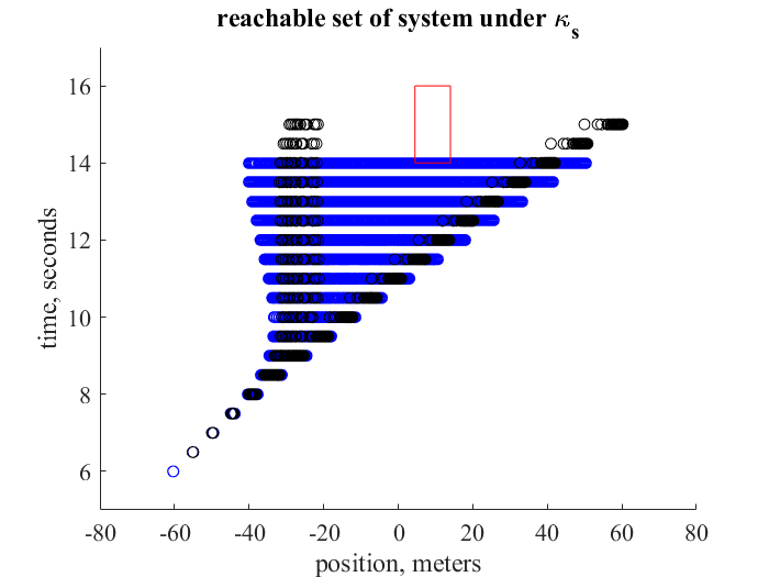
Figure 4. Reachable set and sampled trajectories for the unprotected left turn system with a single neural network planner $\kappa_{s}$. The blue region is the overapproximated reachable set and the black region is 100 sampled trajectories from the same initial set. Initial set $I$ is set as $I=\{x\in\mathbb{R}^{5}|p_{1}\in\left[-60.4\text{, }-60.3\right]\text{, }v_{1}\in\left[10.5\text{, }10.51\right]\text{, }\tau_{min}\equiv 14\text{, }\tau_{max}\equiv 16\text{, }t=6\}$. Unsafe set is $S_{u}=\{x\in\mathbb{R}^{5}|p_{1}\in\left[4.5\text{, }14\right]\text{, }t\in\left[14\text{, }16\right]\}$, and it is marked with a red rectangle.

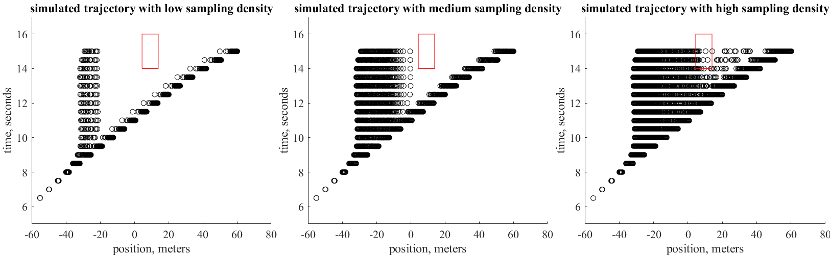
Figure 5. Simulated trajectories with different sampling densities from the initial set $I$, for the unprotected left turn system with a single neural network based planner $\kappa_{s}$. The black region represents simulated trajectories and the red rectangle is the unsafe set $S_{u}$. $I$ and $S_{u}$ are the same as in Fig. 4. From left to right, these three subplots correspond to the trajectories of one hundred, ten thousand and one million samples from the initial set $I$, respectively.

4. Case Studies

Our hierarchical neural network based planner design and safety verification method can be applied to many safety critical systems defined by (2), (3) and (4). In this section, we demonstrate its effectiveness in two case studies of unprotected left turn and highway merging in autonomous driving.

For both applications, we generate the trajectory dataset based on human driving norm and use the same dataset to train all the planning neural networks ($\kappa_{s}\text{, }\mu\text{, }\kappa_{1}\text{, }\kappa_{2}\text{, \ldots, }\kappa_{N}$). These neural networks all have two hidden layers, with each layer having ten neurons. We select ReLU and tanh as the activation functions for the hidden layer and the output layer, respectively. We set control time stepsize $\delta_{c}=0.5$ seconds for all experiments in this work. Based on the verification tool ReachNN (Huang et al., 2019) and POLAR (Huang et al., 2021), we implement Algorithm 1 to compute the overapproximation of reachable set for the system under the single neural network based planner and the hierarchical neural network based planner, respectively.

4.1. Unprotected Left Turn

We conduct experiments for the unprotected left turn system as described earlier in Section 2.

4.1.1. Empirical Study of Single Neural Network Planner

Fig. 4 shows the overapproximated reachable set under a single neural network based planner $\kappa_{s}$, which is consistent with our analysis in Proposition 3.3. We select the initial set $I=\{x\in\mathbb{R}^{5}|p_{1}\in\left[-60.4\text{, }-60.3\right]\text{, }v_{1}\in\left[10.5\text{, }10.51\right]\text{, }\tau_{min}\equiv 14\text{, }\tau_{max}\equiv 16\text{, }t=6\}$ to cover different behaviors (proceed and yield) of vehicle $C1$. The unsafe set $S_{u}$ is determined by $\tau_{min}$ and $\tau_{max}$, i.e., $S_{u}=\{x\in\mathbb{R}^{5}|p_{1}\in\left[4.5\text{, }14\right]\text{, }t\in\left[14\text{, }16\right]\}$. In this figure, the blue region represents the reachable set and the black region is the simulated trajectories of 100 sampling states from the same initial set. The reachable set cannot be represented with several disjoint subsets as described in Eq. (4) and it overlaps with the unsafe set $S_{u}$.

By increasing the number of sampling states from the same initial set $I$, we actually find counterexamples that prove $\kappa_{s}$ is indeed unsafe. Fig. 5 shows the simulated trajectories with different sampling density from $I$. The three subplots from left to right correspond to the trajectories of one hundred, ten thousand and one million samples in the initial set $I$, respectively. Based on our analysis in Proposition 3.3, for any other neural network planner $\kappa^{\prime}_{s}$ that is a convolutional or fully connected neural network with ReLU, sigmoid and tanh activation functions, we can always find counterexamples by increasing the sampling density.

4.1.2. Experiment Results of Hierarchical Planner

For the system with our design of a hierarchical planner $\mu(\kappa_{1}\text{, }\kappa_{2}\text{, }\kappa_{3})$, we compute the overapproximation of the reachable set with the method introduced in Section 3.2, and the results are shown in Figs. 7 and  6.

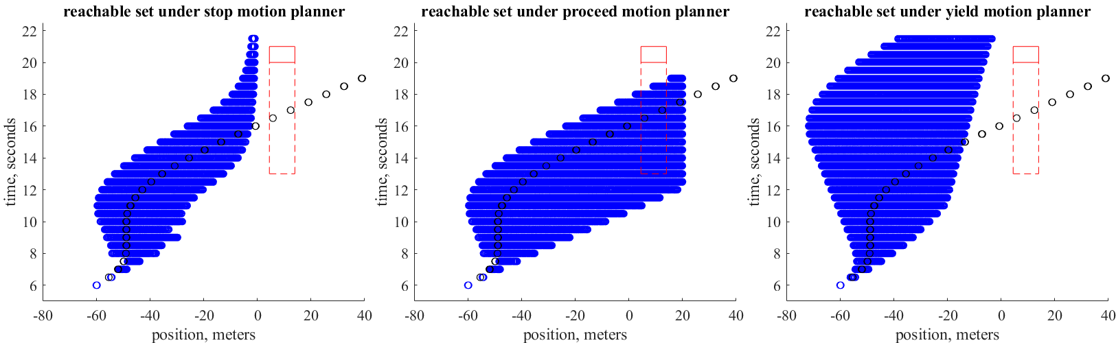
Figure 6. Reachable set and sampled trajectories for the unprotected left turn system under hierarchical neural network planner with changing time window $\left[\tau_{min}\text{, }\tau_{max}\right]$. From left to right, the three subplots present the reachable system states under the stop motion planner, proceed motion planner, and yield motion planner respectively. The blue region is the overapproximated reachable set and the black region is 100 sampled trajectories from the same initial set. Initial set $I$ is set as $I=\{x\in\mathbb{R}^{5}|p_{1}\in\left[-60\text{, }-59.7\right]\text{, }v_{1}\in\left[10.5\text{, }10.51\right]\text{, }\tau_{min}=13\text{, }\tau_{max}=21\text{, }t=6\}$. The time window $\left[\tau_{min}\text{, }\tau_{max}\right]$ is initially $\left[13\text{, }21\right]$ at time $6\leq t<7$, then $\left[15\text{, }21\right]$ at time $7\leq t<8$, $\left[17\text{, }21\right]$ at time $8\leq t<9$, $\left[19\text{, }21\right]$ at time $9\leq t<10$, and finally $\left[20\text{, }21\right]$ at time $t\geq 10$. The unsafe set $S_{u}$ changes with the time window $\left[\tau_{min}\text{, }\tau_{max}\right]$ as time goes on. It is initially the red rectangle with the dashed line and finally the red rectangle with the solid line.

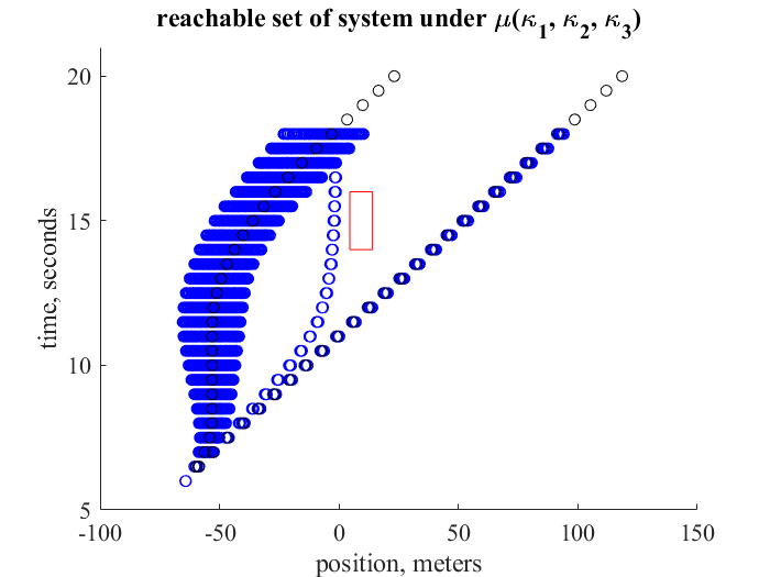
Figure 7. Reachable set and sampled trajectories for the unprotected left turn system with hierarchical neural network planner $\mu(\kappa_{1}\text{, }\kappa_{2}\text{, }\kappa_{3})$. The blue region is the overapproximated reachable set and the black region is 100 sampled trajectories from the same initial set. Initial set $I$ is set as $I=\{x\in\mathbb{R}^{5}|p_{1}\in\left[-64.35\text{, }-64.05\right]\text{, }v_{1}\in\left[10.5\text{, }10.51\right]\text{, }\tau_{min}\equiv 14\text{, }\tau_{max}\equiv 16\text{, }t=6\}$. Unsafe set is $S_{u}=\{x\in\mathbb{R}^{5}|p_{1}\in\left[4.5\text{, }14\right]\text{, }t\in\left[14\text{, }16\right]\}$, and it is marked with a red rectangle. States in the initial set $I$ is assessed by the behavior planner $\mu$ and in this example $S_{ctrl}$ includes all three behaviors (proceed, yield and stop). At the following time steps, vehicle $C1$ will not adjust its behavior and the reachable set of different behaviors are computed independently.

First, we assume that $\tau_{min}$ and $\tau_{max}$ do not change over time. We set the initial set $I=\{x\in\mathbb{R}^{5}|p_{1}\in\left[-64.35\text{, }-64.05\right]\text{, }v_{1}\in\left[10.5\text{, }10.51\right]\text{, }\tau_{min}\equiv 14\text{, }\tau_{max}\equiv 16\text{, }t=6\}$ to cover different behaviors (proceed and yield) of vehicle $C1$. Then the unsafe set is $S_{u}=\{x\in\mathbb{R}^{5}|p_{1}\in\left[4.5\text{, }14\right]\text{, }t\in\left[14\text{, }16\right]\}$. As shown in Fig. 7, due to overapproximation, all three behaviors are included in the reachable set $S_{ctrl}$ by the behavior planner $\mu$ at the beginning. Since the motion estimation for the other vehicle $C2$ remains the same, we assume that the behavior planner is triggered only once. From the figure, we can observe three disjoint reachable subsets in the time interval $t\in\left[10\text{, }16\right]$ and the reachable set has no overlap with the red unsafe region. Thus the planner $\mu(\kappa_{1}\text{, }\kappa_{2}\text{, }\kappa_{3})$ is verified to be safe in this example.

We then consider the case where vehicle $C1$ updates the motion estimation for vehicle $C2$ as the two vehicles get closer to the intersection (which is often the case in practice), and we verify the system safety with the same hierarchical planner. Fig. 6 presents the system state reachable sets under different motion planners $\{R^{\kappa_{1}}\text{, }R^{\kappa_{2}}\text{, }R^{\kappa_{3}}\}$, which all together form the reachable set $R$ under our hierarchical planner. We set the initial set $I=\{x\in\mathbb{R}^{5}|p_{1}\in\left[-60\text{, }-59.7\right]\text{, }v_{1}\in\left[10.5\text{, }10.51\right]\text{, }\tau_{min}=13\text{, }\tau_{max}=21\text{, }t=6\}$. The time window $\left[\tau_{min}\text{, }\tau_{max}\right]$ is initially $\left[13\text{, }21\right]$ at time $6\leq t<7$, then $\left[15\text{, }21\right]$ at time $7\leq t<8$, $\left[17\text{, }21\right]$ at time $8\leq t<9$, $\left[19\text{, }21\right]$ at time $9\leq t<10$, and finally $\left[20\text{, }21\right]$ at time $t\geq 10$. The unsafe set $S_{u}$ changes with the time window $\left[\tau_{min}\text{, }\tau_{max}\right]$ as time goes on. In Fig. 6, the red rectangle with dashed line is the initial unsafe region, and the red rectangle with solid line is the final unsafe region. As there is no overlap between the reachable set with unsafe region, the planner $\mu(\kappa_{1}\text{, }\kappa_{2}\text{, }\kappa_{3})$ is verified to be safe in this case where $C1$ updates its estimation on $C2$ and the time window $\left[\tau_{min}\text{, }\tau_{max}\right]$ is updated over time.

Since the behavior planner is triggered multiple times in the case in Fig. 6, the eventual reachable set $R$ includes system trajectories under switched motion planners and is significantly larger than the reachable set in Fig. 7. Intuitively, if the behavior planner is triggered more frequently, the vehicle $C1$ can adapt to a more appropriate behavior sooner, but this will also results in a larger reachable set and more verification effort.

4.2. Highway Merging

Another common and challenging task for autonomous driving is highway merging. As shown in Fig. 8, vehicle $C1$ intends to merge onto the highway from on-ramp while another vehicle $C2$ stays on the highway. The system can be modeled as follows:

(8) $$\begin{cases}\dot{p}_{1}(t)=v_{1}(t)\\ \dot{v}_{1}(t)=u(t)\\ \dot{p}_{2}(t)=v_{2}(t)\\ \dot{v}_{2}(t)=0\end{cases}$$

where $p_{1}(t)$, $v_{1}(t)$, $p_{2}(t)$ and $v_{2}(t)$ are the longitudinal position and the velocity of vehicle $C1$ and $C2$, respectively. $u(t)$ is the control input, which is the acceleration of vehicle $C1$. In this example, we assume that vehicle $C2$ is a heavy truck and will maintain its speed.

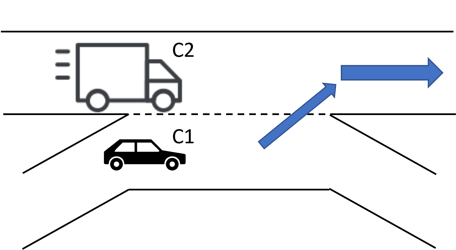
Figure 8. The highway merging system. Vehicle $C1$ is merging onto the highway and vehicle $C2$ stays on the highway. Depending on the positions and velocities of vehicle $C1$ and $C2$, vehicle $C1$ may yield to vehicle $C2$, or proceed.

To simplify this problem, we only discuss longitudinal motion of vehicle $C1$. Merging is considered to be feasible and safe if the longitudinal distance $|p_{1}(t_{x})-p_{2}(t_{x})|$ is larger than a threshold $d_{th}$ at some time point $t_{x}$ when vehicle $C1$ has not reached the end of the side road, i.e, $p_{1}(t_{x})<p_{end}=150$ meters. Different from the unprotected left turn case, the unsafe set $S_{u}$ is not fixed here. The system is safe as long as there exists a position window $\left[p_{1,min}\text{, }p_{1,max}\right]$ for vehicle $C1$ and unsafe set $S_{u}=\{x\in\mathbb{R}^{4}||p_{1}(t)-p_{2}(t)|\leq d_{th}\text{, }p_{1}(t)\in\left[p_{1,min}\text{, }p_{1,max}\right]\}$ such that $S_{u}\cap R=\emptyset$ and $0\leq p_{1,min}\textless p_{1,max}\leq p_{end}$. We select the initial set $I=\{x\in\mathbb{R}^{4}|p_{1}=0\text{, }v_{1}=25\text{, }p_{2}\in\left[-24.5\text{, }-23.5\right]\text{, }v_{2}\in\left[24.5\text{, }25.5\right]\}$ such that vehicle $C1$ may need to choose different behaviors according to the system state.

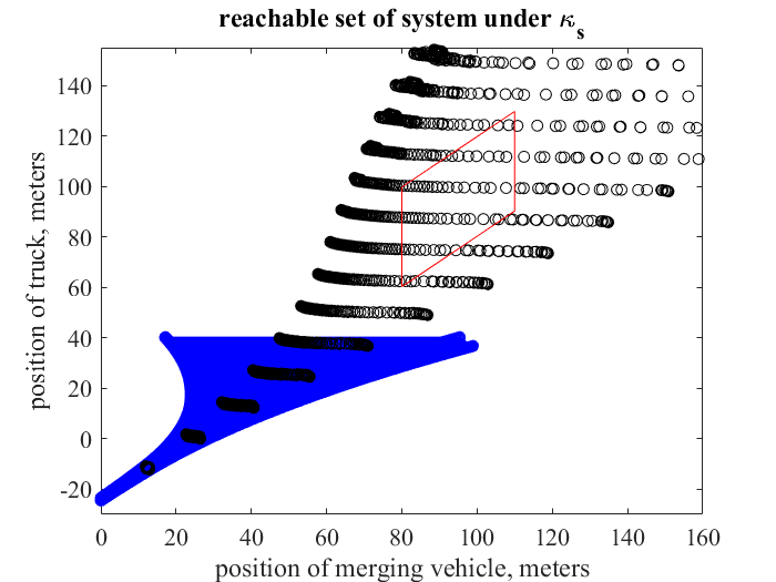
Figure 9. Reachable set and sampled trajectories for the highway merging system under a single neural network planner $\kappa_{s}$. Due to the increasing approximation error, reachability analysis is interrupted and the blue region only shows an overapproximated subset of the reachable set where the position of truck $p_{2}$ is within 40 meters. The black region is 100 sampled trajectories from the same initial set $I=\{x\in\mathbb{R}^{4}|p_{1}=0\text{, }v_{1}=25\text{, }p_{2}\in\left[-24.5\text{, }-23.5\right]\text{, }v_{2}\in\left[24.5\text{, }25.5\right]\}$. An example of unsafe set is $S_{u}=\{x\in\mathbb{R}^{4}||p_{1}(t)-p_{2}(t)|\leq 19.75\text{, }p_{1}(t)\in\left[80\text{, }110\right]\}$, and it is marked with a red parallelogram.

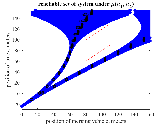
Figure 10. Reachable set and sampled trajectories for the highway merging system under a hierarchical neural network planner $\mu(\kappa_{1}\text{, }\kappa_{2})$. The blue region is the overapproximated reachable set and the black region is 100 sampled trajectories from the same initial set $I=\{x\in\mathbb{R}^{4}|p_{1}=0\text{, }v_{1}=25\text{, }p_{2}\in\left[-24.5\text{, }-23.5\right]\text{, }v_{2}\in\left[24.5\text{, }25.5\right]\}$. In this case, we can find an unsafe set $S_{u}=\{x\in\mathbb{R}^{4}||p_{1}(t)-p_{2}(t)|\leq 19.75\text{, }p_{1}(t)\in\left[80\text{, }110\right]\}$, and it is marked with a red parallelogram. Since $S_{u}\cap R=\emptyset$, vehicle $C1$ can safely merge onto the highway when $p_{1}(t)\in\left[80\text{, }110\right]$.

4.2.1. Empirical Study of Single Neural Network Planner

Similarly as the unprotected left turn case study, we first consider the highway merging system under a single neural network planner $\kappa_{s}$, and Fig. 9 shows the overapproximated reachable set in this case. The reachability analysis is interrupted due to increasing approximation error, and thus the blue region only shows the a subset of the reachable set where the position of truck $p_{2}$ is within 40 meters. This is consistent with our analysis that extremely large Lipschitz constant in this case may greatly increase the difficulty in verification. The black region is the sampled trajectories, which should be strictly covered by the reachable set (if it were computed). From this figure, we cannot find an unsafe set $S_{u}$ that has no overlap with the reachable set, and the system is analyzed to be unsafe under the planner $\kappa_{s}$.

4.2.2. Experiment Results of Hierarchical Planner

We then consider the highway merging system under our design of a hierarchical neural network based planner $\mu(\kappa_{1}\text{, }\kappa_{2})$. We use the same method in Section 3.2 to compute the overapproximation of the reachable set in this case, as shown in Fig. 10. We assume that the behavior planner $\mu$ is triggered only once at the beginning. The left and right branch correspond to yield and proceed behavior of vehicle $C1$, respectively. We can find an unsafe region marked by a red parallelogram, $S_{u}=\{x\in\mathbb{R}^{4}||p_{1}(t)-p_{2}(t)|\leq 19.75\text{, }p_{1}(t)\in\left[80\text{, }110\right]\}$. Since this $S_{u}$ has no overlap with the overapproximated reachable set, vehicle $C1$ can safely merge into the highway when $p_{1}(t)\in\left[80\text{, }110\right]$. This case study once again demonstrates the verifiability and safety of our hierarchical neural network planner.

5. Conclusions

We presented a hierarchical neural network based planner design based on the underlying physical scenarios of the system, and developed novel overapproximation techniques for the reachability analysis of such hierarchical design to ensure system safety. Through theoretical analysis, we showed that our hierarchical design can improve the safety and verifiability for systems that may evolve into different physical scenarios, compared with single neural network based planners. Through two case studies of unprotected left turn and highway merging in autonomous driving, we further demonstrate such advantages empirically.

References

- (1)
- Cao et al. (2020a) Zhangjie Cao, Erdem Bıyık, Woodrow Z Wang, Allan Raventos, Adrien Gaidon, Guy Rosman, and Dorsa Sadigh. 2020a. Reinforcement learning based control of imitative policies for near-accident driving. arXiv preprint arXiv:2007.00178 (2020).
- Cao et al. (2020b) Zhong Cao, Diange Yang, Shaobing Xu, Huei Peng, Boqi Li, Shuo Feng, and Ding Zhao. 2020b. Highway exiting planner for automated vehicles using reinforcement learning. IEEE Transactions on Intelligent Transportation Systems (2020).
- Chen et al. (2019) Jianyu Chen, Bodi Yuan, and Masayoshi Tomizuka. 2019. Deep imitation learning for autonomous driving in generic urban scenarios with enhanced safety. arXiv preprint arXiv:1903.00640 (2019).
- Chen et al. (2020) Yize Chen, Yuanyuan Shi, and Baosen Zhang. 2020. Input convex neural networks for optimal voltage regulation. arXiv preprint arXiv:2002.08684 (2020).
- Dong et al. (2020) Jiqian Dong, Sikai Chen, Yujie Li, Runjia Du, Aaron Steinfeld, and Samuel Labi. 2020. Facilitating connected autonomous vehicle operations using space-weighted information fusion and deep reinforcement learning based control. arXiv preprint arXiv:2009.14665 (2020).
- Dutta et al. (2019) Souradeep Dutta, Xin Chen, and Sriram Sankaranarayanan. 2019. Reachability analysis for neural feedback systems using regressive polynomial rule inference. In Proceedings of the 22nd ACM International Conference on Hybrid Systems: Computation and Control. 157–168.
- Fan et al. (2020) David D Fan, Jennifer Nguyen, Rohan Thakker, Nikhilesh Alatur, Ali-akbar Agha-mohammadi, and Evangelos A Theodorou. 2020. Bayesian learning-based adaptive control for safety critical systems. In 2020 IEEE International Conference on Robotics and Automation (ICRA). IEEE, 4093–4099.
- Fan et al. (2019) Jiameng Fan, Chao Huang, Wenchao Li, Xin Chen, and Qi Zhu. 2019. Towards verification-aware knowledge distillation for neural-network controlled systems. In 2019 IEEE/ACM International Conference on Computer-Aided Design (ICCAD). IEEE, 1–8.
- Farag (2019) Wael Farag. 2019. Complex trajectory tracking using PID control for autonomous driving. International Journal of Intelligent Transportation Systems Research (2019), 1–11.
- Fisac et al. (2018) Jaime F Fisac, Andrea Bajcsy, Sylvia L Herbert, David Fridovich-Keil, Steven Wang, Claire J Tomlin, and Anca D Dragan. 2018. Probabilistically safe robot planning with confidence-based human predictions. arXiv preprint arXiv:1806.00109 (2018).
- Ha et al. (2020) Paul Young Joun Ha, Sikai Chen, Jiqian Dong, Runjia Du, Yujie Li, and Samuel Labi. 2020. Leveraging the capabilities of connected and autonomous vehicles and multi-agent reinforcement learning to mitigate highway bottleneck congestion. arXiv preprint arXiv:2010.05436 (2020).
- Henzinger et al. (1998) Thomas A Henzinger, Peter W Kopke, Anuj Puri, and Pravin Varaiya. 1998. What’s decidable about hybrid automata? Journal of computer and system sciences 57, 1 (1998), 94–124.
- Huang et al. (2021) Chao Huang, Jiameng Fan, Xin Chen, Wenchao Li, and Qi Zhu. 2021. POLAR: A Polynomial Arithmetic Framework for Verifying Neural-Network Controlled Systems. arXiv preprint arXiv:2106.13867 (2021).
- Huang et al. (2019) Chao Huang, Jiameng Fan, Wenchao Li, Xin Chen, and Qi Zhu. 2019. Reachnn: Reachability analysis of neural-network controlled systems. ACM Transactions on Embedded Computing Systems (TECS) 18, 5s (2019), 1–22.
- Huang et al. (2020) Chao Huang, Shichao Xu, Zhilu Wang, Shuyue Lan, Wenchao Li, and Qi Zhu. 2020. Opportunistic intermittent control with safety guarantees for autonomous systems. In 2020 57th ACM/IEEE Design Automation Conference (DAC). IEEE, 1–6.
- Ivanov et al. (2019) Radoslav Ivanov, James Weimer, Rajeev Alur, George J Pappas, and Insup Lee. 2019. Verisig: verifying safety properties of hybrid systems with neural network controllers. In Proceedings of the 22nd ACM International Conference on Hybrid Systems: Computation and Control. 169–178.
- Li et al. (2021) Jinning Li, Liting Sun, Masayoshi Tomizuka, and Wei Zhan. 2021. A Safe Hierarchical Planning Framework for Complex Driving Scenarios based on Reinforcement Learning. arXiv preprint arXiv:2101.06778 (2021).
- Liu et al. (2020a) Xiangguo Liu, Neda Masoud, and Qi Zhu. 2020a. Impact of sharing driving attitude information: A quantitative study on lane changing. In 2020 IEEE Intelligent Vehicles Symposium (IV). IEEE, 1998–2005.
- Liu et al. (2020b) Xiangguo Liu, Guangchen Zhao, Neda Masoud, and Qi Zhu. 2020b. Trajectory planning for connected and automated vehicles: Cruising, lane changing, and platooning. arXiv preprint arXiv:2001.08620 (2020).
- Lu and Hong (2019) Renzhi Lu and Seung Ho Hong. 2019. Incentive-based demand response for smart grid with reinforcement learning and deep neural network. Applied energy 236 (2019), 937–949.
- Ma et al. (2021) Haitong Ma, Jianyu Chen, Shengbo Eben Li, Ziyu Lin, Yang Guan, Yangang Ren, and Sifa Zheng. 2021. Model-based Constrained Reinforcement Learning using Generalized Control Barrier Function. arXiv preprint arXiv:2103.01556 (2021).
- Markolf et al. (2020) Lukas Markolf, Jan Eilbrecht, and Olaf Stursberg. 2020. Trajectory Planning for Autonomous Vehicles combining Nonlinear Optimal Control and Supervised Learning. IFAC-PapersOnLine 53, 2 (2020), 15608–15614.
- Naveed et al. (2020) Kaleb Ben Naveed, Zhiqian Qiao, and John M Dolan. 2020. Trajectory Planning for Autonomous Vehicles Using Hierarchical Reinforcement Learning. arXiv preprint arXiv:2011.04752 (2020).
- Nosrati et al. (2018) Masoud S Nosrati, Elmira Amirloo Abolfathi, Mohammed Elmahgiubi, Peyman Yadmellat, Jun Luo, Yunfei Zhang, Hengshuai Yao, Hongbo Zhang, and Anas Jamil. 2018. Towards practical hierarchical reinforcement learning for multi-lane autonomous driving. (2018).
- Pettet et al. (2020) Geoffrey Pettet, Ayan Mukhopadhyay, Mykel Kochenderfer, and Abhishek Dubey. 2020. Hierarchical Planning for Resource Allocation in Emergency Response Systems. arXiv preprint arXiv:2012.13300 (2020).
- Qureshi et al. (2020) Ahmed Hussain Qureshi, Yinglong Miao, Anthony Simeonov, and Michael C Yip. 2020. Motion planning networks: Bridging the gap between learning-based and classical motion planners. IEEE Transactions on Robotics (2020).
- Seidman et al. (2020) Jacob H Seidman, Mahyar Fazlyab, Victor M Preciado, and George J Pappas. 2020. Robust deep learning as optimal control: Insights and convergence guarantees. In Learning for Dynamics and Control. PMLR, 884–893.
- Stock et al. (2015) Sebastian Stock, Masoumeh Mansouri, Federico Pecora, and Joachim Hertzberg. 2015. Online task merging with a hierarchical hybrid task planner for mobile service robots. In 2015 IEEE/RSJ International Conference on Intelligent Robots and Systems (IROS). IEEE, 6459–6464.
- Tran et al. (2019) Hoang-Dung Tran, Feiyang Cai, Manzanas Lopez Diego, Patrick Musau, Taylor T Johnson, and Xenofon Koutsoukos. 2019. Safety verification of cyber-physical systems with reinforcement learning control. ACM Transactions on Embedded Computing Systems (TECS) 18, 5s (2019), 1–22.
- Tran et al. (2020) Hoang-Dung Tran, Xiaodong Yang, Diego Manzanas Lopez, Patrick Musau, Luan Viet Nguyen, Weiming Xiang, Stanley Bak, and Taylor T. Johnson. 2020. NNV: The Neural Network Verification Tool for Deep Neural Networks and Learning-Enabled Cyber-Physical Systems. In 32nd International Conference on Computer-Aided Verification (CAV).
- Tuncali et al. (2018) Cumhur Erkan Tuncali, James Kapinski, Hisahiro Ito, and Jyotirmoy V Deshmukh. 2018. Reasoning about safety of learning-enabled components in autonomous cyber-physical systems. In Proceedings of the 55th Annual Design Automation Conference. 1–6.
- Wang et al. (2020b) Jingke Wang, Yue Wang, Dongkun Zhang, Yezhou Yang, and Rong Xiong. 2020b. Learning hierarchical behavior and motion planning for autonomous driving. arXiv preprint arXiv:2005.03863 (2020).
- Wang et al. (2021) Yixuan Wang, Chao Huang, Zhilu Wang, Shichao Xu, Zhaoran Wang, and Qi Zhu. 2021. Cocktail: Learn a Better Neural Network Controller from Multiple Experts via Adaptive Mixing and Robust Distillation. arXiv preprint arXiv:2103.05046 (2021).
- Wang et al. (2020a) Yixuan Wang, Chao Huang, and Qi Zhu. 2020a. Energy-efficient control adaptation with safety guarantees for learning-enabled cyber-physical systems. In 2020 IEEE/ACM International Conference On Computer Aided Design (ICCAD). IEEE, 1–9.
- Wei et al. (2017) Tianshu Wei, Yanzhi Wang, and Qi Zhu. 2017. Deep reinforcement learning for building HVAC control. In Proceedings of the 54th annual design automation conference 2017. 1–6.
- Zeng et al. (2019) Wenyuan Zeng, Wenjie Luo, Simon Suo, Abbas Sadat, Bin Yang, Sergio Casas, and Raquel Urtasun. 2019. End-to-end interpretable neural motion planner. In Proceedings of the IEEE/CVF Conference on Computer Vision and Pattern Recognition. 8660–8669.
- Zheng et al. (2017) Stephan Zheng, Yisong Yue, and Patrick Lucey. 2017. Generating long-term trajectories using deep hierarchical networks. arXiv preprint arXiv:1706.07138 (2017).
- Zhou et al. (2019) Mofan Zhou, Yang Yu, and Xiaobo Qu. 2019. Development of an efficient driving strategy for connected and automated vehicles at signalized intersections: a reinforcement learning approach. IEEE Transactions on Intelligent Transportation Systems 21, 1 (2019), 433–443.
- Zhu et al. (2021) Qi Zhu, Chao Huang, Ruochen Jiao, Shuyue Lan, Hengyi Liang, Xiangguo Liu, Yixuan Wang, Zhilu Wang, and Shichao Xu. 2021. Safety-assured design and adaptation of learning-enabled autonomous systems. In 2021 26th Asia and South Pacific Design Automation Conference (ASP-DAC). IEEE, 753–760.