Copula-Based Modeling of RIS-Assisted Communications: Outage Probability Analysis

Abstract

Statistical characterization of the signal-to-noise ratio (SNR) of reconfigurable intelligent surface (RIS)-assisted communications in the presence of phase noise is an important open issue. In this letter, we exploit the concept of copula modeling to capture the non-standard dependence features that appear due to the presence of discrete phase noise. In particular, we consider the outage probability of RIS systems in Rayleigh fading channels and provide joint distributions to characterize the dependencies due to the use of finite resolution phase shifters at the RIS. Numerical assessments confirm the validity of closed-form expressions of the outage probability and motivate the use of bivariate copula for further RIS studies.

I Introduction

Reconfigurable intelligent surfaces (RISs) have recently received remarkable attention as a revolutionary technology for the next generation of wireless communications to provide higher quality of service and spectrum efficiency [1]. It consists of arrays of passive reflecting elements able to introduce specific phase shifts on the impinging signal [2], [3], [4]. Attracted by the appealing advantages of RIS, most works focused on the phase shift matrix design with/without the transmit beamforming to achieve optimal performance and maximum reliability (​​[1] and references therein). The influence of phase noise due to low-resolution quantization and imperfect channel estimation has also been investigated in [4]-​​[10]. In particular, a power scaling analysis in [8] showed that using 2 or 3-bit phase shifters is practically sufficient to achieve close-to-optimal performance. However, there are very few works that derived the outage probability of RIS-aided communication systems in the presence of phase noise. To name a few, the central limit theorem (CLT) was utilized to approximate the RIS channel as a point-to point Nakagami fading channel in [7]. In [9], the authors presented a rough asymptotic outage approximation under the consideration of one bit phase quantization and the non-realistic assumption of perfect independence between the signal components. Despite the large effort, however, the exact outage probability considering $b$-bit phase quantization is still not available in the open literature. The paucity of this investigation is mainly due to the mathematical intricacy of handling the cascaded fading channels of the RIS the existence of non-standard dependence features between the received signal components caused by discrete phase noise. To address this open issue, we utilize the concept of copula modeling to study the impact of the joint distribution of the outage probability. In fact, copulas allow modeling general dependency structures and have already been used in the area of communications [11], [12], [13]
To the best of our knowledge, there has been no previous work applying the copula theory to investigate the performance of RIS-assisted communications. In the previous works, either CLT analysis [7] or asymptotic formulation [5], [9] are suggested for RIS with phase noise. However, the channel models proposed in the absence of phase noise have to be further simplified to tractable formulation as shown in for example [14], where the composite channel gain is approximated by the Gamma distribution. Unlike previous works, we use copula modeling to realize the non-linear dependence structure that appears due to phase noise. As such, we characterize the joint distribution and propose tractable model based on copulas. Using copula model, we derive closed-form outage probabilities considering general $b$-bit phase quantization. Our results provide a solid basis for future studies of and system design of RIS-assisted networks.

II System Model

In this paper, we consider an RIS-aided system, which consists of a single-antenna transmitter, an RIS equipped with $M$ elements, and a single-antenna receiver. The RIS dynamically adjusts the reflecting coefficient of each element to reconfigure the incident signal with the desired phase shift. Thus, the received signal at the receiver is written as

$$y=\sqrt{lp_{t}}{\bf h}{\bf\Phi}{\bf g}s+{z}_{1},$$ (1)

where ${z}_{1}$ represents thermal noise with power $\sigma^{2}$, $p_{t}$ is the transmit power, and $l$ is the equivalent path-loss of the RIS link, which is composed of a forward channel from the transmitter to the RIS and a backward channel from the RIS to the receiver, denoted by ${\bf h}\in{\cal C}^{M\times 1}$ and ${\bf g}\in{\cal C}^{1\times M}$, respectively. We assume that all the channels in the system undergo independent Rayleigh fading, and the instantaneous channel state information (CSI) for all links is assumed to be available at the receiver and RIS. Hence, the RIS is expected to intelligently reconfigure the wireless channel by varying a quantized phase matrix ${\bf\Phi}$ defined as

$${\mathbb{\Phi}}=\Big{\{}e^{j\phi_{n}},\phi_{n}\in\Big{\{}0,\frac{2\pi}{L},\ldots,\frac{2\pi(L-1)}{L}\Big{\}}\Big{\}},$$ (2)

where $L=2^{b}$, with $b\geq 1$, is the number of discrete phases that can be generated by the RIS subject to hardware complexity and power consumption [10],[4].
In practice, the phase shifts of the reconfigurable elements of an RIS cannot be optimized with an arbitrary precision because of the finite number of quantization bits used or possible errors in estimating the phases of fading channels. In this case, the phase of the $i$-th element of the RIS can be written as $\phi_{i}=-\angle{h_{i}}-\angle{g_{i}}+\theta_{i}$, where $\theta_{i}$ denotes a random phase noise, which is assumed to be i.i.d. in this paper. Thus, the equivalent channel observed by the receiver is a complex random variable and the SNR is

$$\gamma=\rho\left|\sum_{i=1}^{M}|h_{i}||g_{i}|e^{j\theta_{i}}\right|^{2},$$ (3)

where $\rho=l\rho_{S}$ with $\rho_{S}=\frac{p_{t}}{\sigma^{2}}$ denoting the transmit SNR and $\theta_{i}$ represents the phase error which is uniformly distributed over $[-\pi/L,\pi/L]$. To the best of our knowledge, characterising the distribution of (3) as the key to the outage analysis of the RIS-aided system is not straightforward, and it is the first endeavor in this paper.

III A Brief Review of Copula Theory

Copula as a novel method to model correlated random variables (RVs) [11], enables the computation of the joint distributions of these RVs from their marginal PDFs. Each copula function is defined by a particular dependence parameter which indicates the intensity of dependency.

Definition 1.

(Copula) A copula is an $n$-dimensional distribution function with standard uniform marginals.

The practical relevance of copulas stems from Sklar’s theorem, which we restate in the following.

Theorem 1.

(Sklar’s Theorem [11]). Let $F(x_{1},x_{2},\ldots,x_{n})$ be an $n$-dimensional joint cumulative distribution function of random variables $(x_{1},x_{2},\ldots,x_{n})$ with marginal CDFs $F_{1}(x_{1}),\ldots,F_{n}(x_{n})$. Then there exists a copula $C$ such that,

$$F(x_{1},\ldots,x_{n})=C(F_{1}(x_{1}),\ldots,F_{n}(x_{n})),$$ (4)

for all $x_{i}\in\mathbb{R}$. Furthermore, if $F(x_{i})$ is continuous for all $i=1,\dots,n$, then $C$ is unique.

Although many types of copulas have been defined so far, we exploit the Farlie Gumbel-Morgenstern (FGM) copula function [12] to analyze the performance metrics of the considered RIS-assisted system. The generalized FGM copula of $n$-dimension is defined as

$$\!\!\!\!\!\!\!\!C(u_{1},\ldots,u_{n})$$ (5)

$$\!\!\!\!\!\!\!\!\!\!\!\!\!\!\!\!\!\!\!\!\!\!\!\!\!\!\!\!\!\!\!\!\!\!\!\!\!\!\!\!\!\!\!\!\!\!=u_{1}u_{2}\ldots u_{n}\left(\!\!1+\sum_{k=2}^{n}\sum_{1\leq j_{1}\leq\ldots\leq j_{n}}\!\!\!\!\!\!\!\!\Theta_{j_{1}j_{2}\ldots,j_{n}}{\tilde{u}}_{1}{\tilde{u}}_{2}\ldots{\tilde{u}}_{n}\!\!\right),$$

where ${\tilde{u}}=1-u$ and $\Theta\in[-1,1]$ is a dependence structure parameter of the FGM copula.

IV Outage Probability Analysis Based on FGM Copula

Here, we provide an FGM copula based construction of bivariate random variables with arbitrary dependency. This construction is then used to derive the outage probability (OP) and unveil the impact of the joint distribution and the dependency on its performance.
The OP is defined as the probability that the instantaneous SNR $\gamma$ fall below a determined threshold $\gamma_{th}$, namely,

$${\cal O}_{p}\!=\!{\rm P}\left(\!\rho\left|\sum_{i=1}^{M}|h_{i}||g_{i}|e^{j\theta_{i}}\right|^{2}\!\!\leq\!\gamma_{th}\!\right)={\rm P}\!\left(\!{X^{2}}\!+\!{Y^{2}}\!\leq\!\rho_{t}\!\right),$$ (6)

where $\rho_{t}={\gamma_{th}}/{\rho}$ , $X=\sum_{i=1}^{M}|h_{i}||g_{i}|\cos(\theta_{i})$ and $Y=\sum_{i=1}^{M}|h_{i}||g_{i}|\sin(\theta_{i})$. In (6), the real part and the imaginary part of the received signal through the RIS are separated. We note that $X$ and $Y$ exhibit generalized dependence structures beyond the simple linear correlation concept widely used in wireless communications. Moreover, considering the randomness of $X$ and $Y$ and using the transformation of random variables, the outage probability can be formulated as

$${\cal O}_{p}=\int_{0}^{\rho_{t}}\int_{0}^{\sqrt{\rho_{t}-x}}\frac{1}{\sqrt{x}}f_{X,Y}\left(\sqrt{x},y\right)dxdy,$$ (7)

where $f_{X,Y}\left(x,y\right)$ is the joint PDF of $X$ and $Y$. Next, we exploit the FGM Copula to construct the joint distribution $f_{X,Y}\left(x,y\right)$ .

Proposition 1.

The copula-based joint distribution of $X$ and $Y$ under one-bit quantization is obtained as

$$f_{X,Y}(x,y) = \frac{e^{-x-|y|}x^{M-1}}{2^{M}\Gamma(M)^{2}}$$ (8)

$$\!\!\!\!\!\!\!\!\!\!\!\!\!\!\!\!\!\!\!\!\!\!\!\!\!\!\!\!\!\!\!\!\!\!\!\!\!\!\!\!\!\times\sum_{k=0}^{M-1}\frac{(M-1+k)!|y|^{M-1+k}}{2^{k}k!(M-1-k)!}\Bigg{(}1+\Theta\left(1-\frac{2\Gamma(M,x)}{\Gamma(M)}\right)$$

$$\!\!\!\!\!\!\!\!\!\!\!\!\!\!\!\!\!\!\!\!\!\!\!\!\!\!\!\!\!\!\!\!\!\!\!\!\!\!\!\!\!\times\left(1-\frac{1}{2^{M-1}\Gamma(M)}\!\!\sum_{k=0}^{M-1}\!\!\frac{(M-1+k)!\Gamma(M-k,y)}{2^{k-1}k!(M-1-k)!}\right)\!\Bigg{)},$$

where $\Theta\in[-1,1]$ and $\Gamma(a,z)$ stands for the incomplete Gamma function [16].

Proof.

Using the copula theory and (4), the corresponding joint PDF can be obtained as follows:

$$f_{X,Y}(x,y) = \frac{d^{2}C(F_{X}(x),F_{Y}(y))}{dxdy}$$ (9)

$$\overset{(a)}{=} c(F_{X}(x),F_{Y}(y))f(x)f(y),$$

where $(a)$ follows by utilizing the concept of Chain rule with $f_{X}(x)$ and $f_{Y}(y)$ being the marginal pdfs of $X$ and $Y$, respectively, and $c(F_{X}(x),F_{Y}(y))$ denotes the bivariate Copula density function obtained from (5) as

$$\!\!\!c(F_{X}(x),F_{Y}(y))=1+\Theta\left(\left(2F_{X}(x)\!-\!1\right)\left(2F_{Y}(y)\!-\!1\right)\right).$$ (10)

We assume that each element of the RIS is a one-bit phase shifter, then considering the phase errors $\theta_{i}$, $i\in\{1,\ldots,M\}$ are mutually independent and uniformly distributed on the interval $[$-$\pi/2,\pi/2]$, the marginal distributions of $X$ and $Y$ can be obtained, by following the rationale presented in Appendix A, as

$$f_{X}(x)=\frac{e^{-x}x^{M-1}}{\Gamma(M)},\quad x\geq 0,$$ (11)

and

$$f_{Y}(y)=\frac{e^{-|y|}}{2^{M}\Gamma(M)}\sum_{k=0}^{M-1}\frac{(M-1-k)!|y|^{M-1+k}}{2^{k}k!(M-1-k)!},\quad y\in\mathbb{R}$$ (12)

while the CDFs of $X$ and $Y$ can be obtained as

$$F_{X}(x)=1-\frac{\Gamma(M,x)}{\Gamma(M)},$$ (13)

and

$$\!\!\!F_{Y}(y)=1-\frac{1}{2^{M}\Gamma(M)}\sum_{k=0}^{M-1}\frac{(M-1+k)!\Gamma(M-k,y)}{2^{k}k!(M-1-k)!}.$$ (14)

Hence, plugging (13)-(14) back into (10) and then substituting (10)-(12) into (9) complete the proof. ∎

Proposition 2.

When the RIS uses one-bit phase shifters, the outage probability in Rayleigh fading is given by (15), shown at the top of this page,

$${\cal O}_{p} = \frac{\rho_{t}^{M/2}(1+\Theta)}{2\sqrt{\pi}\Gamma(M)}{\rm H}_{0,1:1,1,1,2}^{0,0:1,1,2,1}\Bigg{[}\begin{array}[]{ccc}\sqrt{\rho_{t}}\\ \sqrt{\rho_{t}}\end{array}\Bigg{|}\begin{array}[]{ccc}-:(1\!-\!\frac{M}{2},\frac{1}{2});(0,2)\\ (-\frac{M}{2};\frac{1}{2},2)\!:\!(0,1);(0,2),(M-\frac{1}{2},2)\end{array}\Bigg{.}\Bigg{]}$$ (34)

$$-\frac{\rho_{t}^{M/2}\Theta}{2\sqrt{\pi}\Gamma(M)^{2}}{\rm H}_{0,1:2,2,1,2}^{0,0:2,2,2,1}\Bigg{[}\begin{array}[]{ccc}\sqrt{\rho_{t}}\\ \sqrt{\rho_{t}}\end{array}\!\!\Bigg{|}\begin{array}[]{ccc}-:\!(M,1),(1-\frac{M}{2},\frac{1}{2});(0,2)\\ (-\frac{M}{2};\frac{1}{2},2):(0,1),(M,1);(0,2),(M\!-\!\frac{1}{2},2)\end{array}\Bigg{.}\Bigg{]}$$

$$+\frac{\Theta\rho_{t}^{M/2}}{2^{3M}\Gamma(M)^{2}}\!\!\!\sum_{k=0}^{M-1}\sum_{t=0}^{M-1}\sum_{p=0}^{M-t-1}\frac{\Gamma(M\!+\!k)\Gamma(M\!-\!t)}{2^{2k+t+p}k!t!p!\Gamma(M\!-\!k)}\Bigg{(}\!\!{\rm H}_{0,1:1,1,1,2}^{0,0:1,1,2,1}\Bigg{[}\!\!\!\begin{array}[]{ccc}\sqrt{\rho_{t}}\\ 2\sqrt{\rho_{t}}\end{array}\!\!\Bigg{|}\begin{array}[]{ccc}-:(1-\frac{M}{2},\frac{1}{2});(1,1)\\ (0;\frac{1}{2},\frac{1}{2}):(0,1);(M\!+\!k\!+\!p,1),(0,1)\end{array}\Bigg{.}\Bigg{]}$$

$$\!-\!2{\rm H}_{0,1:2,2,1,2}^{0,0:2,2,2,1}\Bigg{[}\begin{array}[]{ccc}\!\!\!\!\sqrt{\rho_{t}}\\ \!\!2\sqrt{\rho_{t}}\!\!\end{array}\!\!\Bigg{|}\begin{array}[]{ccc}-:(M,1),(1\!-\!\frac{M}{2},\frac{1}{2});(1,1)\\ (0;\frac{1}{2},\frac{1}{2})\!:\!(0,1),(M,1);(0,1),(M\!+\!k\!+\!p,1)\end{array}\Bigg{.}\Bigg{]}\Bigg{)},$$

where $H[\cdot,\cdot]$ is the bivariate Fox’s H-function [15, Eq. (2.56)], for which several efficient implementations have been reported in the literature [4].

Proof.

Using the copula-based joint distribution in Proposition 1 and resorting to $\Gamma(n,x)=\Gamma(n)e^{-x}\sum_{k=0}^{n-1}\frac{x^{k}}{k!}$, the inner integral in (7) can be evaluated, yielding

$${\cal O}_{p}\!\!\! = \!\!\!\int_{0}^{\rho_{t}}\frac{f_{X}(\sqrt{x}){\cal K}(\Theta,x)}{2\sqrt{\pi}\Gamma(M)\sqrt{x}}{\rm G}_{0,2}^{2,0}\Bigg{[}\frac{\rho_{t}\!-\!x}{4}\Bigg{|}\begin{array}[]{ccc}-\\ 0,M\!-\!\frac{1}{2}\end{array}\Bigg{.}\!\!\Bigg{]}dx$$ (38)

$$\!\!\!\!\!\!\!\!\!\!\!\!\!\!\!+\int_{0}^{\rho_{t}}\frac{f_{X}(\sqrt{x})}{\sqrt{x}}\left({\cal K}(\Theta,x)-1\right)B(\sqrt{\rho_{t}-x})dx,$$

where ${\cal K}(\Theta,x)=1+\Theta\left(2F_{X}(\sqrt{x})-1\right)$, and

$$\!\!\!\!B(z) = \frac{1}{2^{3M}\Gamma(M)^{2}}\sum_{k=0}^{M-1}\sum_{t=0}^{M-1}\sum_{p=0}^{M-t-1}$$ (41)

$$\!\!\!\!\!\!\!\!\!\!\!\!\!\!\!\!\!\!\!\!\!\!\!\!\!\!\!\!\!\!\!\frac{(M-1+k)!(M-1-t)!}{2^{2k+t+p}k!t!p!(M-1-k)!}{\rm G}_{1,2}^{1,1}\Bigg{[}2z\Bigg{|}\begin{array}[]{ccc}1\\ M+k+p,0\end{array}\Bigg{.}\!\!\Bigg{]},$$

with ${\rm G}(\cdot)$ being the Meijer’s G function [16]. Now substituting (11)-(13) into (38), recognizing that $\exp(-\sqrt{x})=\frac{1}{2\pi j}\int_{{\cal L}}\Gamma(s)x^{-s/2}ds$, $\Gamma(a,\sqrt{x})=\frac{1}{2\pi j}\int_{{\cal L}}\frac{\Gamma(a+s)\Gamma(s)}{\Gamma(1+s)}x^{-s/2}ds$ and [16, Eq. (9.301)] and then utilizing [16, Eq.(3.194.1)], the outage probability follows from applying [15, Definiton A.1], which completes the proof. ∎

Corollary 1.

The asymptotic (for high-SNR) outage probability of an RIS-aided system under one-bit quantization can be formulated as ${\cal O}_{p}\underset{\rho\rightarrow\infty}{\approx}({\cal G}_{c}\rho)^{-{\cal G}_{d}}$, where ${\cal G}_{d}=\frac{M}{2}$ denotes the diversity order and ${\cal G}_{c}=\frac{\Gamma(M-\frac{1}{2})}{2\sqrt{\pi}(1+\frac{M}{2})\Gamma(M)}$ denotes the coding gain.

Proof.

It follows by using the asymptotic expansion of Mellin-Barnes integrals of the bivariate Fox’s H functions in (15) near zero by applying [17, Eq. (1.8.4] and by keeping only the dominant terms using [17, Eq. (1.8.7)]. ∎

In the most general case, i.e., for an arbitrary choice of quantization level $L$ and generalized fading model, the marginal densities and distributions of $X$ and $Y$ are either unknown or expressed in terms of infinite integrals [10, Appendix A]. In this case, the copula-based joint density become much more complex. To circumvent this problem, we combine, hereafter, both copula and Gamma modeling.

Lemma 1.

Letting $Z\in\{X,Y\}$, the distribution of $Z^{2}$ can be accurately approximated by the Gamma PDF with shape and scale parameters given by $\kappa_{Z}$ and $\beta_{Z}$ as

$$Z^{2}\simeq\Gamma(\kappa_{Z},\beta_{Z}),$$ (42)

where $\kappa_{Z}=\frac{\mathbb{E}(Z^{2})^{2}}{\mathbb{E}(Z^{4})-\mathbb{E}(Z^{2})^{2}}$ and $\beta_{Z}=\frac{\kappa_{Z}}{\mathbb{E}(Z^{2})}$.

Proof.

In order to approximate $Z^{2},Z\in\{X,Y\}$ being a Gamma random variable, we have to find the shape and scale parameters (i.e., $\kappa_{Z}$, $\beta_{Z}$) based on the statistical information of $Z$. To this end, we use two different moments of $Z$ i.e., $\mathbb{E}(Z^{2})$ and $\mathbb{E}(Z^{4})$ to find the parameters $\kappa_{Z}$ and $\beta_{Z}$. First, from the definitions of $X$ and $Y$, we have

$$X^{2}=\sum_{i=1}^{M}z_{i}^{2}\cos(\theta_{i})^{2}+\sum_{i=1}^{M}\sum_{j=1,j\neq i}^{M}z_{i}z_{j}\cos(\theta_{i})\cos(\theta_{j}),$$ (43)

and

$$Y^{2}=\sum_{i=1}^{M}z_{i}^{2}\sin(\theta_{i})^{2}+\sum_{i=1}^{M}\sum_{j=1,j\neq i}^{M}z_{i}z_{j}\sin(\theta_{i})\sin(\theta_{j}),$$ (44)

where $z_{i}=|h_{i}||g_{i}|$. Since $|h_{i}|$ and $|g_{i}|$ undergo i.i.d. unit variance Rayleigh fading, we have $\mathbb{E}(z_{i})=\frac{\pi}{4}$, $\mathbb{E}(z_{i}^{2})=1$, $\mathbb{E}(z_{i}^{3})=\frac{9\pi}{16}$, and $\mathbb{E}(z_{i}^{4})=4$. Moreover, since $\theta_{i}$ is a uniform random variable with PDF $f_{\theta}(x)=\frac{L}{2\pi}$, $-\frac{\pi}{L}\leq x\leq\frac{\pi}{L}$, we obtain

$$\mathbb{E}(Z^{2})=\begin{cases}M\left(\frac{1}{2}\!+\!\frac{1}{2}\rm{sinc}\left(\frac{2\pi}{L}\right)\!+\!\frac{(M-1)L^{2}}{16}\sin^{2}\left(\frac{\pi}{L}\right)\right)&Z=X;\\ M\left(\frac{1}{2}-\frac{1}{2}\rm{sinc}\left(\frac{2\pi}{L}\right)\right)&Z=Y,\end{cases}$$ (45)

Next, in order to find the moment $\mathbb{E}(Z^{4})$, we initially expand it as

$$\mathbb{E}(Z^{4}) = \mathbb{E}\left[\left(\sum_{i=1}^{M}d_{i}^{2}\right)^{2}\right]+2\sum_{l=1}^{M}\sum_{i=1}^{M}\sum_{j=1,j\neq i}^{M}\mathbb{E}\left[d_{l}^{2}d_{i}d_{j}\right]$$ (46)

$$+\mathbb{E}\left[\left(\sum_{i=1}^{M}\sum_{j=1,i\neq j}^{M}d_{i}d_{j}\right)^{2}\right],$$

where $d_{i}=z_{i}\cos(\theta_{i})$ if $Z=X$ or $d_{i}=z_{i}\sin(\theta_{i})$ if $Z=Y$. The first term on the rights side of (46) can be expressed as

$$\mathbb{E}\left[\left(\sum_{i=1}^{M}d_{i}^{2}\right)^{2}\right]=\sum_{i=1}^{M}\mathbb{E}\left[d_{i}^{4}\right]+\sum_{i=1}^{M}\sum_{j=1,j\neq i}^{M}\mathbb{E}\left[d_{i}^{2}d_{j}^{2}\right],$$ (47)

which, after some manipulations, can be rewritten as

$$\mathbb{E}\left[\left(\sum_{i=1}^{M}d_{i}^{2}\right)^{2}\right]=\begin{cases}\frac{M}{16\pi^{2}}(A\!+B)&Z=X;\\ \frac{M}{16\pi^{2}}(B-A)&Z=Y,\end{cases}$$ (48)

where $A=4\pi(3\!+\!M)L\sin\left(\frac{2\pi}{L}\right)$ and $B=\!L^{2}(M\!-\!1)\sin^{2}\left(\frac{2\pi}{L}\right)\!+\!2\pi\left(2(5\!+\!M)\pi\!+\!L\sin\left(\frac{4\pi}{L}\right)\right)$. The second term of (46) can be expressed as (49), as shown at the top of this page. Further, the third term of (46) can be expressed as (50), as shown at the top of the this page. Finally, after plugging (48), (49) and (50) back into (46) and using (45) and several simplifications, Lemma 1 is proved.

$$\begin{array}[]{l}2\sum\limits_{l=1}^{M}{\sum\limits_{m=1}^{M}{\sum\limits_{n=1,n\neq m}^{M}{{\mathbb{E}}\left[{d_{l}^{2}{d_{m}}{d_{n}}}\right]}}}=4\sum\limits_{m=1}^{M}{\sum\limits_{n=1,n\neq m}^{M}{{\mathbb{E}}\left[{d_{m}^{3}{d_{n}}}\right]}}+2\sum\limits_{l=1}^{M}{\sum\limits_{m=1,m\neq l}^{M}{\sum\limits_{n=1,n\neq m}^{M}{{\mathbb{E}}\left[{d_{l}^{2}{d_{m}}{d_{n}}}\right]}}}\\ =\begin{cases}\frac{1}{{64\pi}}M\left({M-1}\right){L^{2}}{\sin^{2}}\left({\frac{\pi}{L}}\right)\left((11+4M)\pi+3\pi\cos\left({\frac{2\pi}{L}}\right)+2L(M-1)\sin\left({\frac{2\pi}{L}}\right)\right)&Z=X;\\ 0&Z=Y,\end{cases}\end{array}$$ (49)

$$\begin{array}[]{l}{\mathbb{E}}\left[{{{\left({\sum\limits_{m=1}^{M}{\sum\limits_{n=1,n\neq m}^{N}{{d_{m}}{d_{n}}}}}\right)}^{2}}}\right]=\sum\limits_{j=1}^{M}{\sum\limits_{l=1,l\neq m}^{M}{{{\mathbb{E}}\left[{d_{j}^{2}d_{l}^{2}}\right]}}}+\sum\limits_{l=1}^{M}{\sum\limits_{m=1,m\neq l}^{M}{\sum\limits_{n=m+1,n\neq l}^{N}{{\mathbb{E}}\left[{d_{l}^{2}{d_{m}}{d_{n}}}\right]}}}\\ +\sum\limits_{j=1}^{M}{\sum\limits_{l=1,l\neq j\neq m\neq n}^{M}{\sum\limits_{m=1,l\neq j\neq m\neq n}^{M}{\sum\limits_{n=1,l\neq j\neq m\neq n}^{M}{{\mathbb{E}}\left[{{d_{j}}{d_{l}}{d_{m}}{d_{n}}}\right]}}}}\\ =\begin{cases}\frac{M(M-1)}{256\pi^{2}}\left(8L^{2}(M-1)\pi^{2}\sin\left(\frac{\pi}{L}\right)^{2}+8\pi L^{3}(M-1)\sin\left(\frac{\pi}{L}\right)^{3}\cos\left(\frac{\pi}{L}\right)\right)&Z=X;\\ +L^{4}\left(6-5M+M^{2}\right)\pi^{2}\sin\left(\frac{\pi}{L}\right)^{4}+16\left(2\pi+L\sin\left(\frac{2\pi}{L}\right)\right)^{2}\\ \frac{M^{2}\left(L\sin\left({\frac{2\pi}{L}}\right)-2\pi\right)^{2}}{16\pi^{2}}&Z=Y,\end{cases}\end{array}$$ (50)

∎

Proposition 3.

A copula-based joint distribution of $X^{2}$ and $Y^{2}$ under $b$-bits phase quantization and Rayleigh fading is given by

$$f_{X^{2},Y^{2}}(x,y) = \frac{e^{-\frac{x}{\beta_{X}}-\frac{y}{\beta_{Y}}}x^{\kappa_{X}-1}y^{\kappa_{Y}-1}}{\Gamma(\kappa_{X})\Gamma(\kappa_{Y})\beta_{X}^{\kappa_{X}}\beta_{Y}^{\kappa_{Y}}}$$ (51)

$$\!\!\!\!\!\!\!\!\!\!\!\!\!\!\!\!\!\!\!\!\!\!\!\!\!\!\!\!\!\!\!\!\!\!\!\!\!\!\!\!\!\!\!\!\!\!\!\!\left(1+\Theta\left(1-\frac{2\Gamma(\kappa_{X},\frac{x}{\beta_{X}})}{\Gamma(\kappa_{X})}\right)\left(1-\frac{2\Gamma(\kappa_{Y},\frac{y}{\beta_{Y}})}{\Gamma(\kappa_{Y})}\right)\right).$$

Proof.

The proof follows in the same line of (8) using the Gamma model approximation of $X^{2}$ and $Y^{2}$ in Lemma 1 after recognizing that $f_{Z}(z)=\frac{e^{-\frac{z}{\beta_{Z}}}z^{\kappa_{Z}-1}}{\Gamma(\kappa_{Z})\beta_{Z}^{\kappa_{Z}}}$ and $F_{Z}(z)=1-\frac{\Gamma(\kappa_{Z},\frac{z}{\beta_{Z}})}{\Gamma(\kappa_{Z})}$, $Z\in\{X^{2},Y^{2}\}$. ∎

Proposition 4.

The outage probability of RIS-assisted system with $b$-bit phase quantization can be expressed as

$$\!{\cal O}_{p}\!\!\!\! = \!\!\!\!\!\int_{0}^{\rho_{t}}\!\!f_{X^{2}}(x)\left(\Theta{\cal G}(x)+1\right)\left(1-\frac{\Gamma\left(\kappa_{Y},\frac{\rho_{t}-x}{\beta_{Y}}\right)}{\Gamma(\kappa_{Y})}\right)dx$$ (56)

$$-2\Theta\int_{0}^{\rho_{t}}\frac{{\cal G}(x)f_{X^{2}}(x)}{\Gamma(\kappa_{Y})}\left(\frac{\rho_{t}-x}{\beta_{Y}}\right)^{\kappa_{Y}}$$

$$\!\!\!\!\!\!\!\!\!\!\!\!\!\!\!\!\!\!\!\!\!\!\!\!\!\!\times{\rm H}_{0,1:0,1,1,2}^{0,0:1,0,2,0}\Bigg{[}\begin{array}[]{ccc}\frac{\rho_{t}-x}{\beta_{Y}}\\ \frac{\rho_{t}-x}{\beta_{Y}}\end{array}\Bigg{|}\begin{array}[]{ccc}-:-;(1,1)\\ \!\!\!(\kappa_{Y},1,1):\!(0,1);(0,1),(\kappa_{Y},1)\end{array}\Bigg{.}\!\!\!\!\Bigg{]}dx,$$

where ${\cal G}(x)=1-\frac{2\Gamma(\kappa_{X},\frac{x}{\beta_{X}})}{\Gamma(\kappa_{X})}$.

Proof.

It follows from substituting (51) into (7) and solving the integral with respect to $y$ by following similar steps as in Proposition 2. ∎

To the best of our knowledge, Propositions 1 and 3, characterize for the fisrt time in the literature the joint distribution between the underlying real and imaginary parts of the received signal through RIS, which due to the presence of phase noise, exhibit arbitrary correlation. This finding allows us to derive the exact outage probability for different quantization levels, as shown in Proposition 2 and 4 for the first disclosure.
It is worth noting that other performance metrics, including the ergodic capacity, error probability and secrecy rate, also depend remarkably on the joint distributions in Propositions 1 and 2. It is therefore of interest to investigate in future research how such dependency structure can be exploited in RIS-aided communications. Moreover, by leveraging fundamental results from the Mellin transform [15] and Copula [12] theories, it is possible to extend the current framework to deal with inherent complexities due to generalized fading models such as general multi-path with/without specular component (LOS) and shadowing.

V Numerical Results

In Fig. 1 (a), we show the outage probability for the RIS-aided system under the condition of one-bit phase quantization as described in Proposition 2. It can be observed that the Monte-Carlo simulation of the outage probability matches the copula-based closed-form expression in Proposition 2. Notice that our approach outperforms the Nakagami-m approximation in [7], which is degraded for low outage values. Fig. 1 (a) further illustrates that the copula-based asymptotic analysis is very accurate showing that the diversity order is indeed $M/2$.

In Fig. 1 (b), the behavior of the outage probability based on variations of $M$ and $b$ for selected values of the dependence parameter $\Theta$ is illustrated. We examine the closeness between the simulated values of the outage and the approximations based on the the Gamma model presented in Proposition 4. Fig. 1 (b) corroborates the fact that increasing both $M$ and $b$ improves the performance of the RIS system. In particular, it is shown that using 2 bit phase shifters is practically sufficient to achieve close-to-optimal performance with only approximately $0.9$ dB power loss, which is consistent with [8, Proposition 1].

Denoting the distances to and from the RIS as $l_{1}$, $l_{2}$, the equivalent path-loss of the RIS link can be written as $l=(l_{1}l_{2})^{-\nu}$, where $\nu$ is the path-loss exponent. In Fig. 1 (c), we investigate the outage probability for different geographical deployments of the RIS which is allowed to move along the horizontal line between the transmitter and the receiver. An observation from Fig. 1 (c), which agrees with the finding in [10], is that the RIS has increased outage as it moves far away from either the transmitter or the receiver. It is also noticed from Fig. 1 (b) and (c) that copula is more accurate for positive dependence structure i.e., when $\Theta\in(0,1]$.

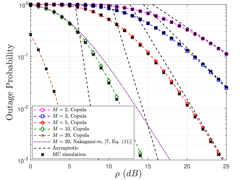
(a)

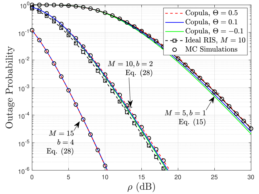
(b)

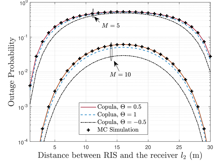
(c)

Figure 1: The outage probability with $\gamma_{th}=5$ dB under (a) one-bit phase quantization with dependence parameter $\theta=0.55$. (b) $b$-bit quantization for different $M$ and $\Theta$ values. (c) one-bit quantization for different positions of the RIS with $p_{t}/\sigma^{2}=15$ dB and $\nu=2.8$.

VI Conclusion

In this letter, we developed a theoretical framework to analyze the outage probability of RIS-aided systems with phase noise in which copulas are exploited to capture the non-linear dependence among the signal components. When a one-bit phase shifter is used at each reflective element, we obtained the expression of the outage probability using the bivariate Fox’s H function. To deal with the complicated scenario where the RIS employs $b$-bit phase shifters, we amalgamated both copula and Gamma modeling to efficiently compute the outage probability. Our results are the foundations of any further study that relies on the joint density and cumulative probability functions of the underlying variables pertaining to the received signal via low resolution RIS.

VII Appendix A

As noted earlier, $\theta_{i}$ is uniformly distributed on the interval $[-\frac{\pi}{2},\frac{\pi}{2}]$. As a result, the PDF of $v_{i}=\cos(\phi_{i})$ is given by

$$f_{v_{i}}(v)=\frac{2}{\pi\sqrt{1-v^{2}}},\quad\text{for~{}}0\leq v\leq 1.$$ (58)

Recall that both forward and backward channels of the RIS-aided system follow i.i.d. Rayleigh fading $f_{y_{i}}(x)=2x{\rm{e}}^{-x^{2}}$, $y\in\{h,g\}$, using (58), the PDF of $x_{i}=h_{i}g_{i}v_{i}$ can be calculated as

$$f_{x_{i}}(z)=\int_{0}^{\infty}\frac{1}{x}f_{h_{i}}(x)f_{g_{i}v_{i}}\left(\frac{z}{x}\right)\textrm{d}x,$$ (59)

where

$$f_{g_{i}v_{i}}\left(x\right)=\frac{4}{\pi}\int_{0}^{1}\frac{\rm{e}^{-\frac{x^{2}}{z^{2}}}}{z^{2}\sqrt{1-z^{2}}}\textrm{d}z.$$ (60)

Hence the pdf of $x_{i}$ is obtained as $f_{x_{i}}(x)=\exp(-x).$ Similarly, the PDF of $y_{i}=h_{i}g_{i}\sin(\theta_{i})$ is $f_{y_{i}}(y)=\frac{1}{2}\exp(-|y|)$. Since the sum of independent exponentially distributed random variables with the same mean is Gamma-distributed, we can obtain easily the PDFs of $X=\sum_{i=1}^{M}x_{i}$ and $Y=\sum_{i=1}^{M}y_{i}$ as given in (11) and (12), respectively.

References

• [1] Y. Liu, X. Liu, X. Mu, T. Hou, J. Xu, M. D. Renzo, N. Al-Dhahir., “Reconfigurable Intelligent Surfaces: Principles and Opportunities” IEEE Communications Surveys & Tutorials., Early Access, May 5, 2021, doi: 10.1109/COMST.2021.3077737.
• [2] M. Di Renzo et al., “Smart radio environments empowered by reconfigurable intelligent surfaces: How it works, state of research, and the road ahead,” IEEE J. Sel. Areas Commun., vol. 38, no. 11, pp. 2450-2525, Nov. 2020.
• [3] Q. Wu, R. Zhang, “Intelligent Reflecting Surface Enhanced Wireless Network via Joint Active and Passive Beamforming”, IEEE Trans. Wireless Communications, vol. 18, no. 11, Nov 2019.
• [4] I. Trigui, W. Ajib, W.-P. Zhu, M. Di Renzo, ”Performance evaluation and diversity analysis of RIS-assisted communications over generalized fading channels in the presence of phase noise”. 2020, [Online]. Available: arxiv.org/abs/2011.12260.
• [5] K. Zhi, C. Pan , H. Ren , and K. Wang., “Uplink Achievable Rate of Intelligent Reflecting Surface-Aided Millimeter-Wave Communications With Low-Resolution ADC and Phase Noise,” IEEE Wireless Commun. Letter, vol. 10, no. 3, 2021.
• [6] X. Qian, M. D. Renzo , J. Liu , A. Kammoun , and M. S. Alouini “Beamforming Through Reconfigurable Intelligent Surfaces in Single-User MIMO Systems: SNR Distribution and Scaling Laws in the Presence of Channel Fading and Phase Noise,” IEEE Wireless Commun. Letter, vol. 10, no. 1, 2021.
• [7] M. A. Badiu and J. P. Coon, “Communication through a large reflecting surface with phase errors,” IEEE Wireless Commun. Lett., vol. 9, no. 2, pp. 184–188, Feb. 2020.
• [8] Q. Wu and R. Zhang, ”Beamforming optimization for wireless network aided by intelligent reflecting surface with discrete phase shifts,” IEEE Trans. Commun.,vol. 68, no. 3, pp. 1838-1851, 2020.
• [9] T. Wang, G. Chen, J. P. Coon, and M.-A. Badiu, ”Study of intelligent reflective surface assisted communications with one-bit phase adjustments,” IEEE Global Communications Conference, pp. 7-11, Dec 2020.
• [10] I. Trigui, E. K. Agbogla, M. Benjillali, W. Ajib, and W. P. Zhu, “Bit Error Rate Analysis for Reconfigurable Intelligent Surfaces with Phase Errors,” IEEE Commun. Letters, vol. 25, no. 7, 2021.
• [11] R. B. Nelsen, An Introduction to Copulas. New York, NY, USA: Springer, 2007
• [12] P. Bickel, P. Diggle, S. Fienberg, U. Gather, I. Olkin, S. Zeger, Copula Theory and Its Applications, Springer, 2009.
• [13] F. R. Ghadi and G. A. Hodtani, “Copula-Based Analysis of Physical Layer Security Performances Over Correlated Rayleigh Fading Channels,” IET Commun., vol. 16, pp. 431–440, 2021.
• [14] Z. Xie, W. Yi, X. Wu, Y. Liu, and A. Nallanathan, ”STAR-RIS aided NOMA in multi-cell networks: A general analytical framework with gamma distributed channel modeling,” [Online]. Available: https://arxiv.org/abs/2108.06704
• [15] A. M. Mathai, R. K. Saxena, and H. J. Haubold, The H-Function: Theory and Applications, Springer Science & Business Media, 2009.
• [16] I. Gradshteyn and I. Ryzhik, Table of Integrals, Series, and Products, Academic Press, 1994.
• [17] A. Kilbas and M. Saigo, H-Transforms: Theory and Applications, CRC Press, 2004.
• [18] Joe, H.: Multivariate models and dependence concepts, Monographs on Statistics and Applied Probability, vol. 73. Chapman & Hall$/$CRC, New York (2001).