Local well-posedness of a nonlinear Fokker-Planck model

Abstract.

Noise or fluctuations play an important role in the modeling and understanding of the behavior of various complex systems in nature. Fokker-Planck equations are powerful mathematical tools to study behavior of such systems subjected to fluctuations. In this paper we establish local well-posedness result of a new nonlinear Fokker-Planck equation. Such equations appear in the modeling of the grain boundary dynamics during microstructure evolution in the polycrystalline materials and obey special energy laws.

1. Introduction

Fluctuations play an essential role in the modeling and understanding of the behavior of various complex processes. Many natural systems are affected by different external and internal mechanisms that are not known explicitly, and very often described as fluctuations or noise. Fokker-Planck models are widely used as a versatile mathematical tool to describe the macroscopic behavior of the systems that undergo such fluctuations, see more detailed discussion and examples in [40, 20, 15, 27, 7, 6, 14, 26], among many others. In our previous work we derived Fokker-Planck type systems as a part of grain growth models of polycrystalline materials, e.g. [2, 4, 1, 18].

From the thermodynamical point of view, many Fokker-Planck type systems can be viewed as special cases of general diffusion [23]. They can be derived from the kinematic continuity equations, the conservation law, and the specific energy dissipation law, using the energetic variational approaches [37, 23]. We want to point out that while the linear and nonlinear Fokker-Planck models with the energy laws can be obtained using such energetic variational approach, not all Fokker-Planck systems derived from stochastic differential equations (SDEs) by the Ito process have underlying energy law principles [41].

First, consider the following conservation law subject to the natural boundary condition,

(1.1) $$\left\{\begin{aligned} \frac{\partial f}{\partial t}+\nabla\cdot(f\bm{u})&=0,&\quad&t>0,\ x\in\Omega,\\ f\bm{u}\cdot\nu|_{\partial\Omega}&=0,&\quad&t>0.\end{aligned}\right.$$

Here $\Omega\subset\mathbb{R}^{n}$ is a convex domain, $f=f(x,t):\Omega\times[0,T)\rightarrow\mathbb{R}$ is a probability density function, $\bm{u}$ is the velocity vector which depends on $x$, $t$, and the probability density function $f$, and $\nu$ is an outer unit normal to the boundary $\partial\Omega$ of the domain $\Omega$. We assume that the above system (1.1) also satisfies the following energy law,

(1.2) $$\frac{d}{dt}\int_{\Omega}\omega(f,x)\,dx=-\int\pi(f,x,t)|\bm{u}|^{2}\,dx.$$

Here, $\omega=\omega(f,x)$ represents the free energy, which defines the equilibrium state of the system, and $\pi(f,x,t)$ is the so-called mobility function which defines the evolution of the system to the equilibrium state. The specific forms of these quantities will be discussed in more details below. Now, take a formal time-derivative on the left-hand side of (1.2), then using integration by parts together with system (1.1), we get,

(1.3) $$\begin{split}\frac{d}{dt}\int_{\Omega}\omega(f,x)\,dx&=\int_{\Omega}\omega_{f}(f,x)f_{t}\,dx\\ &=-\int_{\Omega}\omega_{f}(f,x)\nabla\cdot(f\bm{u})\,dx=\int_{\Omega}\nabla\omega_{f}(f,x)\cdot(f\bm{u})\,dx.\end{split}$$

Using relations (1.2) and (1.3), we have that,

$$-\int\pi(f,x,t)|\bm{u}|^{2}\,dx=\int_{\Omega}\nabla\omega_{f}(f,x)\cdot(f\bm{u})\,dx.$$

Thus, the velocity field $\bm{u}$ of the model (1.1)-(1.2) should satisfy the following relation,

(1.4) $$-\pi(f,x,t)\bm{u}=f\nabla(\omega_{f}(f,x)).$$

In fact (1.4) represents the force balance equation for the system. The left hand side represents the dissipative force and the right hand side is the conservative force obtained using the free energy of the system. This derivation is consistent with the general energetic variational approach in [37, 23].

Let us put this discussion in the context of linear and nonlinear Fokker-Planck models now.

Such systems arise in many physical and engineering applications, e.g., [11, 12, 2, 4, 1, 18, 34]. One example of the application of Fokker-Planck systems is the modeling of grain growth in polycrystalline materials. Many technologically useful materials appear as polycrystalline microstructures, composed of small monocrystalline cells or grains, separated by interfaces, or grain boundaries of crystallites with different lattice orientations. In a planar grain boundary network, a point where three grain boundaries meet is called a triple junction point, see Fig.  1. Grain growth is a very complex multiscale and multiphysics process influenced by the dynamics of grain boundaries, triple junctions and the dynamics of lattice misorientations (difference in the lattice orientations between two neighboring grains that share the grain boundary, Fig.  1), e.g., [3, 38, 39]. In case of the grain growth modeling [18], in the Fokker-Planck system, $f$ may describe the joint distribution function of the lattice misorientation of the grain boundaries and of the position of the triple junctions, $\phi$ may describe the grain boundary energy density, and $D$ is related to the absolute temperature of the entire system [32] (it can be viewed as a function of the fluctuation parameters of the lattice misorientations and of the position of the triple junctions due to fluctuation-dissipation principle [18]).

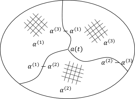
Figure 1. Illustration of the three grain boundaries that meet at a triple junction which is positioned at the $\bm{a}(t)$. Each grain boundary has a lattice misorientation which is the difference between lattice (lined grids on the figure) orientations $\alpha^{(j)},j=1,2,3$ of the grains that share the grain boundary. In [18], a grain boundary network was considered as a system of such triple junctions and the grain boundaries misorientations, and was modeled by the Fokker-Planck equation for the joint distribution function of the position of the triple junctions and the misorientations.

In the cases when $\omega(f,x)=Df(\log f-1)+f\phi$ (free energy density) and $\pi(f,x,t)=f(x,t)$ (mobility), where $D>0$ is a positive constant and the potential function $\phi=\phi(x)$ is a given function. $D$ being a constant is the case of the system with homogeneous absolute temperature [11, 19]. We will recover the corresponding linear Fokker-Planck model from conservation and energy laws, (1.1)-(1.2). First, the direct computation yields,

$$f\nabla\omega_{f}=f\nabla(D\log f+\phi(x)).$$

Hence, from (1.4), the velocity field $\bm{u}$ should be,

(1.5) $$\bm{u}=-\nabla(D\log f+\phi(x))=-\Big{(}D\frac{\nabla f}{f}+\nabla\phi(x)\Big{)}.$$

Using vector field (1.5) in the conservation law (1.1), we obtain the following linear Fokker-Planck equation,

(1.6) $$\frac{\partial f}{\partial t}=\nabla\cdot(\nabla\phi(x)f)+\nabla\cdot(D\nabla f).$$

Note, that the linear Fokker-Planck equation has the associated Langevin equation [41, 21],

(1.7) $$dx=-\nabla\phi(x)dt+\sqrt{2D}dB.$$

The linear Fokker-Planck equation (1.6) can also be derived from the corresponding Langevin equation (1.7) (see [15]).

Some diffusion equations can be interpreted using the idea of Brownian motion [21]. Consider random process

(1.8) $$dx=\upsilon(x)dt+\sigma(x)dB,$$

where $B$ is standard Brownian motion. With a Taylor expansion of probability density function $f(x,t)$, one can obtain the following PDEs:

• Ito calculus provides, $f_{t}+\nabla\cdot(\upsilon f)=\frac{1}{2}\Delta(\sigma^{2}f)$.

• The derivation using Stratonovich integral yields, $f_{t}+\nabla\cdot(\upsilon f)=\frac{1}{2}\nabla\cdot[\sigma\nabla(\sigma f)]$.

• One can also derive PDE with self-adjoint diffusion term, namely, $f_{t}+\nabla\cdot(\upsilon f)=\frac{1}{2}\nabla\cdot[\sigma^{2}\nabla(f)]$.

In many cases, these models can also be treated in the general framework of energetic variational approach. Following the fluctuation-dissipation theorem [13, 30], taking the convection coefficient, $\upsilon(x)=-\frac{1}{2}\sigma(x)^{2}\nabla\phi$, and assuming that $f$ satisfies the conservation law $f_{t}+\nabla\cdot(uf)=0$, the equations above satisfy and can also be obtained from variation of the following energy laws [23],

• For Ito, $\frac{d}{dt}\int_{\Omega}[f\ln(\frac{1}{2}\sigma^{2}f)+\phi f]\,dx=-\int_{\Omega}\frac{f}{\frac{1}{2}\sigma^{2}}|u|^{2}\,dx.$

• For Stratonovich, $\frac{d}{dt}\int_{\Omega}[f\ln(\sigma f)+\phi f]\,dx=-\int_{\Omega}\frac{f}{\frac{1}{2}\sigma^{2}}|u|^{2}\,dx.$

• For self-adjoint case, $\frac{d}{dt}\int_{\Omega}[f\ln f+\phi f]\,dx=-\int_{\Omega}\frac{f}{\frac{1}{2}\sigma^{2}}|u|^{2}\,dx,$

where $\Omega\subset\mathbb{R}^{d}$ is a bounded domain, $d\geq 1$.

In this paper, instead of starting from the stochastic differential equations, we will derive the system from the energetic aspects, by prescribing the kinematic conservation law and the energy dissipation law. We will consider the case of the inhomogeneous absolute temperature and more general dissipation mechanism. In particular, we look at the case with $\omega(f,x)=D(x)f(\log f-1)+f\phi(x)$, and $\pi(f,x,t)=2D(x)f/(b(x,t))^{2}$, where $D=D(x)$ and $\phi=\phi(x)$ are positive functions. The function $b(x,t)$ is also positive, and provides the extra freedom in the dissipation mechanism. As discussed above, such systems may arise in the grain growth modeling, e.g. [18, 17]. In particular, the temperature, in terms of $D$ in this context, will account for some information of the under-resolved mechanisms in the systems, such as critical events/disappearance events (e.g. grain disappearance, facet/grain boundary disappearance, facet interchange, splitting of unstable junctions and nucleation of the grains). The specific form of the mobility function $\pi(f,x,t)$ here is the direct consequence of the fluctuation-dissipation theorem [30, 13, 18], which ensures that the system under consideration will approach the equilibrium configuration.

Since, in this case, the conservative force takes the form

$$f\nabla\omega_{f}=f\nabla(D(x)\log f+\phi(x)).$$

Hence, from (1.4), the velocity field $\bm{u}$ will be,

(1.9) $$\bm{u}=-\frac{(b(x,t))^{2}}{2D(x)}\nabla(D(x)\log f+\phi(x)).$$

Using formula (1.9) in the conservation law (1.1), we obtain the nonlinear Fokker-Planck equation (with energy law as defined in (1.2), see also discussion below in Section 2),

(1.10) $$\frac{\partial f}{\partial t}-\nabla\cdot\left(\frac{(b(x,t))^{2}}{2D(x)}f\nabla(D(x)\log f+\phi(x))\right)=0.$$

Note, that the nonlinearity $f\log f$ in (1.10) comes as a result of inhomogeneity of the absolute temperature $D(x)$. In addition, in contrast with the linear Fokker-Planck model (1.6), the nonlinear Fokker-Planck model does not have the corresponding Langevin equation. Instead it has the associated stochastic differential equation with coefficients that depend on the probability density $f(x,t)$.

This work establishes local well-posedness of the new nonlinear Fokker-Planck type model (1.10) subject to the boundary and initial conditions. Note, inhomogeneity and resulting non-linearity in the new model (1.10) are very different from the vast existing literature on the Fokker-Planck type models. They come as a result of inhomogeneous absolute temperature in a free energy for the system (2.2). Such absolute temperature gives rise to a nonstandard nonlinearity of the form $f\nabla D(x)\log f$ in the corresponding PDE model (see (1.10), or (2.1) in Section 2 below). For example, any conventional entropy methods, including Bakry-Emory method [28] do not extend to such models in a standard or trivial way. In addition models like (1.10) or (2.1) appear as subsystems in the much more complex systems in the grain growth modeling in polycrystalline materials, and hence one needs to know properties of the classical solutions to such PDEs.

The paper is organized as follows. In Section 2, we first state the nonlinear Fokker-Planck system and validate energy law using given partial differential equation and the boundary conditions. After that we show local existence of the solution to the model. In Section 3, we establish uniqueness of the local solution. Some conclusions are given in Section 4.

2. Existence of a local solution

In this section, we will provide a constructive proof of the existence of a local classical solution of the following nonlinear Fokker-Planck type equation with the natural boundary condition (see also (1.10) in Section 1):

(2.1) $$\left\{\begin{aligned} &\frac{\partial f}{\partial t}=-\nabla\cdot\left(\left(-\frac{(b(x,t))^{2}}{2D(x)}\nabla\phi(x)-\frac{(b(x,t))^{2}}{2D(x)}\log f\nabla D(x)\right)f\right)+\frac{1}{2}\nabla\cdot((b(x,t))^{2}\nabla f),\quad x\in\Omega,\ t>0,\\ &\left(\frac{(b(x,t))^{2}}{2D(x)}f\nabla\phi(x)+\frac{(b(x,t))^{2}}{2D(x)}f\log f\nabla D(x)+\frac{1}{2}(b(x,t))^{2}\nabla f\right)\cdot\nu\bigg{|}_{\partial\Omega}=0,\quad t>0,\\ &f(x,0)=f_{0}(x),\quad x\in\Omega,\end{aligned}\right.$$

where $\Omega\subset\mathbb{R}^{d}$ is a bounded domain, $d\geq 1$. Here $b=b(x,t)$ is a positive function on $\Omega\times[0,\infty)$, $D=D(x)$ is a positive function on $\Omega$, $f_{0}=f_{0}(x)$ is a suitable (to be defined later through $\rho_{0}$ in (2.18) and (2.19)) positive probability density function on $\Omega$ and $\phi=\phi(x)$ is a function on $\Omega$. A function $f=f(x,t)>0$ is an unknown probability density function.

The Fokker-Planck equation (2.1) has a dissipative structure for the following free energy,

(2.2) $$F[f]:=\int_{\Omega}\left(D(x)f(x,t)(\log f(x,t)-1)+f(x,t)\phi(x)\right)\,dx.$$

Below, we validate an energy law for the Fokker-Planck equation (2.1) by performing formal calculations.

Proposition 2.1.

Let $b=b(x,t)$, $D=D(x)$, $f_{0}=f_{0}(x)$, $\phi=\phi(x)$ be sufficiently smooth functions. Then a classical solution $f$ of the Fokker-Planck equation (2.1) satisfies the following energy law,

(2.3) $$\frac{d}{dt}F[f]=-\int_{\Omega}\frac{(b(x,t))^{2}}{2D(x)}\left|\nabla(\phi(x)+D(x)\log f(x,t))\right|^{2}f(x,t)\,dx.$$

Proof.

Here, we will validate the energy law via calculation of the rate of change of the free energy $F$ (see also relevant discussion in Section 1 where we postulated the energy law for the model and derived the velocity field, and hence the PDE as a consequence). By direct computation of $\frac{dF}{dt}$ and using the Fokker-Planck equation (2.1) together with $\nabla f=f\nabla\log f$, we have,

(2.4) $$\begin{split}\frac{d}{dt}F[f]&=\int_{\Omega}\left(D(x)\log f(x,t)+\phi(x)\right)\frac{\partial f}{\partial t}(x,t)\,dx\\ &=-\int_{\Omega}\left(D(x)\log f(x,t)+\phi(x)\right)\nabla\cdot(f(x,t)\bm{u})\,dx,\end{split}$$

where we introduced the velocity vector field as,

(2.5) $$\bm{u}:=-\frac{(b(x,t))^{2}}{2D(x)}\nabla\phi(x)-\frac{(b(x,t))^{2}}{2D(x)}\log f(x,t)\nabla D(x)-\frac{1}{2}(b(x,t))^{2}\nabla\log f(x,t).$$

Note that, $\nabla(D(x)\log f(x,t))=\log f(x,t)\nabla D(x)+D(x)\nabla\log f(x,t)$, hence formula (2.5) becomes (1.9). Next, applying integration by parts with the natural boundary condition (2.1), we obtain,

(2.6) $$\int_{\Omega}\left(D(x)\log f(x,t)+\phi(x)\right)\nabla\cdot(f(x,t)\bm{u})\,dx\\ =-\int_{\Omega}\nabla\left(D(x)\log f(x,t)+\phi(x)\right)\cdot(f(x,t)\bm{u})\,dx.$$

From (2.4), (1.9), and (2.6), we obtain the energy law,

$$\frac{d}{dt}F[f]=-\int_{\Omega}\frac{(b(x,t))^{2}}{2D(x)}\left|\nabla\left(\phi(x)+D(x)\log f(x,t)\right)\right|^{2}f(x,t)\,dx.$$

∎

One can observe from the energy law (2.3) that an equilibrium state $f^{\mathrm{eq}}$ for the Fokker-Planck equation (2.1) satisfies $\nabla(\phi(x)+D(x)\log f^{\mathrm{eq}})=0$. Here, we derive the explicit representation of the equilibrium solution for the Fokker-Planck equation (2.1).

Proposition 2.2.

Let $b=b(x,t)$, $D=D(x)$, $f_{0}=f_{0}(x)$, $\phi=\phi(x)$ be sufficiently smooth functions. Then the smooth equilibrium state $f^{\mathrm{eq}}$ for the Fokker-Planck equation (2.1) is given by,

(2.7) $$f^{\mathrm{eq}}(x)=\exp\left(-\frac{\phi(x)-\Cl{const:2.9}}{D(x)}\right),$$

where $\Cr{const:2.9}$ is a constant, which satisfies,

$$\int_{\Omega}\exp\left(-\frac{\phi(x)-\Cr{const:2.9}}{D(x)}\right)\,dx=1.$$

Proof.

We have from the energy law (2.3) that,

$$0=\frac{d}{dt}F[f^{\mathrm{eq}}]=-\int_{\Omega}\frac{(b(x,t))^{2}}{2D(x)}\left|\nabla\left(\phi(x)+D(x)\log f^{\mathrm{eq}}(x)\right)\right|^{2}f^{\mathrm{eq}}(x)\,dx,$$

hence $\nabla\left(\phi(x)+D(x)\log f^{\mathrm{eq}}\right)=0$. Thus, there is a constant $\Cr{const:2.9}$ such that

$$\phi(x)+D(x)\log f^{\mathrm{eq}}(x)=\Cr{const:2.9},$$

and hence

$$f^{\mathrm{eq}}(x)=\exp\left(-\frac{\phi(x)-\Cr{const:2.9}}{D(x)}\right).$$

∎

Remark 2.3.

Note that the nonlinear Fokker-Planck equation (2.1) can also be derived from the dissipation property of the free energy $F[f]$ (2.2) along with the Fokker-Planck equation,

(2.8) $$\frac{\partial f}{\partial t}=-\nabla\cdot\left(\bm{a}(x,t)f\right)+\frac{1}{2}\nabla\cdot\left((b(x,t))^{2}\nabla f\right)$$

subject to the natural boundary condition, $(\bm{a}(x,t)f+\frac{1}{2}(b(x,t))^{2}\nabla f)\cdot\nu|_{\partial\Omega}=0,$ [17]. Let us briefly review the derivation [17]. Indeed, by (2.8) and using the integration by parts, the rate of change of the free energy $\frac{d}{dt}F[f]$ is calculated as,

$$\begin{split}\frac{d}{dt}F[f]&=\int_{\Omega}(D(x)\log f(x,t)+\phi(x))\frac{\partial f}{\partial t}(x,t)\,dx\\ &=-\int_{\Omega}(D(x)\log f(x,t)+\phi(x))\nabla\cdot\left(\left(\bm{a}(x,t)-\frac{1}{2}(b(x,t))^{2}\nabla\log f(x,t)\right)f(x,t)\right)\,dx\\ &=\int_{\Omega}\nabla(D(x)\log f(x,t)+\phi(x))\cdot\left(\bm{a}(x,t)-\frac{1}{2}(b(x,t))^{2}\nabla\log f(x,t)\right)f(x,t)\,dx.\end{split}$$

Since

$$\nabla(D(x)\log f(x,t)+\phi(x))=\log f(x,t)\nabla D(x)+D(x)\nabla\log f(x,t)+\nabla\phi(x),$$

we obtain the energy dissipation estimate as,

$$\frac{d}{dt}F[f]=-\int_{\Omega}\frac{(b(x,t))^{2}}{2D(x)}\left|\nabla(D(x)\log f(x,t)+\phi(x))\right|^{2}f(x,t)\,dx$$

provided the following relation holds,

(2.9) $$\bm{a}(x,t)=-\frac{(b(x,t))^{2}}{2D(x)}\nabla\phi(x)-\frac{(b(x,t))^{2}}{2D(x)}\log f(x,t)\nabla D(x).$$

Note that when $D(x)$ is independent of $x$, $\nabla D(x)=0$ and hence (2.1) becomes a linear Fokker-Planck equation. The relation (2.9) is consistent with the fluctuation-dissipation relation, which should guarantee not only the dissipation property of the free energy $F[f]$, but also that the solution of the nonlinear Fokker-Planck equation (2.1) converges to the equilibrium state $f^{\mathrm{eq}}$ given by (2.7) (see also [18] for more detailed discussion).

Now, let us define the scaled function $\rho$ by taking the ratio of $f$ and $f^{\mathrm{eq}}$ (2.7),

(2.10) $$\rho(x,t)=\frac{f(x,t)}{f^{\mathrm{eq}}(x)},\quad\text{or}\quad f(x,t)=\rho(x,t)f^{\mathrm{eq}}(x)=\rho(x,t)\exp\left(-\frac{\phi(x)-\Cr{const:2.9}}{D(x)}\right).$$

This auxiliary function was also employed in [28, Theorem 2.1] to study long-time asymptotics of the solutions of linear Fokker-Planck equations. Here, we will use the scaled function $\rho$ as a part of local well-posedness study. Hence, below, we will reformulate the nonlinear Fokker-Planck equation (2.1) into a model for the scaled function $\rho$. We have,

$$f^{\mathrm{eq}}\frac{\partial\rho}{\partial t}=\nabla\cdot\left(\frac{(b(x,t))^{2}}{2D(x)}f^{\mathrm{eq}}\rho\left(\nabla\phi(x)+\log(f^{\mathrm{eq}}\rho)\nabla D(x)+D(x)\nabla\log(f^{\mathrm{eq}}\rho)\right)\right).$$

Next, using the equilibrium state (2.7), we have,

$$\nabla D(x)\log f^{\mathrm{eq}}+D(x)\nabla(\log f^{\mathrm{eq}})+\nabla\phi(x)=0.$$

In addition, note that $\log\rho\nabla D(x)+D(x)\nabla\log\rho=\nabla(D(x)\log\rho)$. Thus, the scaled function $\rho$ satisfies,

$$f^{\mathrm{eq}}\frac{\partial\rho}{\partial t}=\nabla\cdot\left(\frac{(b(x,t))^{2}}{2D(x)}f^{\mathrm{eq}}\rho\nabla\left(D(x)\log\rho\right)\right).$$

Employing the property of the equilibrium state (2.7) again, the natural boundary condition (2.1) becomes,

$$\left(\frac{(b(x,t))^{2}}{2D(x)}f^{\mathrm{eq}}\rho\nabla\left(D(x)\log\rho\right)\right)\cdot\nu\bigg{|}_{\partial\Omega}=0.$$

Therefore, the nonlinear Fokker-Planck equation (2.1) transforms into the following initial-boundary value problem for $\rho$ defined in (2.10),

(2.11) $$\left\{\begin{aligned} &f^{\mathrm{eq}}(x)\frac{\partial\rho}{\partial t}=\nabla\cdot\left(\frac{(b(x,t))^{2}}{2D(x)}f^{\mathrm{eq}}(x)\rho\nabla\left(D(x)\log\rho\right)\right),&\quad&x\in\Omega,\ t>0,\\ &\left(\frac{(b(x,t))^{2}}{2D(x)}f^{\mathrm{eq}}(x)\rho\nabla\left(D(x)\log\rho\right)\right)\cdot\nu\bigg{|}_{\partial\Omega}=0,&\quad&t>0,\\ &\rho(0,x)=\rho_{0}(x)=\frac{f_{0}(x)}{f^{\mathrm{eq}}(x)},&\quad&x\in\Omega.\end{aligned}\right.$$

Next, the free energy (2.2) and the energy law (2.3) can also be stated in terms of $\rho$. Using $D(x)\log f^{\mathrm{eq}}(x)=-\phi(x)+\Cr{const:2.9}$ from (2.7), we obtain,

(2.12) $$F[f]=\int_{\Omega}\left(D(x)(\log\rho-1)+\Cr{const:2.9}\right)\rho f^{\mathrm{eq}}(x)\,dx,$$

and,

(2.13) $$\frac{d}{dt}F[f]=-\int_{\Omega}\frac{(b(x,t))^{2}}{2D(x)}\left|\nabla(D(x)\log\rho)\right|^{2}\rho f^{\mathrm{eq}}(x)\,dx.$$

Thus, it is clear from (2.12)-(2.13) that weighted $L^{2}$ space, $L^{2}(\Omega,f^{\mathrm{eq}}(x)\,dx)$ can play an important role in studying the equation (2.11) (see for example, [35, 18]).

However, hereafter, we study a classical solution for the problem (2.11), and we consider Hölder spaces and norms as defined below. We give now the notion of a classical solution of the problem (2.11).

Definition 2.4.

A function $\rho=\rho(x,t)$ is a classical solution of the problem (2.11) in $\Omega\times[0,T)$ if $\rho\in C^{2,1}(\Omega\times(0,T))\cap C^{1,0}(\overline{\Omega}\times[0,T))$, $\rho(x,t)>0$ for $(x,t)\in\Omega\times[0,T)$, and satisfies equation (2.11) in a classical sense.

To state assumptions and the main result, we also define the parabolic Hölder spaces and norms. For the Hölder exponent $0<\alpha<1$, the time interval $T>0$, and the function $f$ on $\Omega\times[0,T)$, we define the supremum norm $\|f\|_{C(\Omega\times[0,T))}$, the Hölder semi-norms $[f]_{\alpha,\Omega\times[0,T)}$, and $\langle f\rangle_{\alpha,\Omega\times[0,T)}$ as,

(2.14) $$\begin{split}\|f\|_{C(\Omega\times[0,T))}&=\sup_{x\in\Omega,\ t\in[0,T)}|f(x,t)|,\\ [f]_{\alpha,\Omega\times[0,T)}&:=\sup_{x,x^{\prime}\in\Omega,\ t\in[0,T)}\frac{|f(x,t)-f(x^{\prime},t)|}{|x-x^{\prime}|^{\alpha}},\\ \langle f\rangle_{\alpha,\Omega\times[0,T)}&:=\sup_{x\in\Omega,\ t,t^{\prime}\in[0,T)}\frac{|f(x,t)-f(x,t^{\prime})|}{|t-t^{\prime}|^{\alpha}},\end{split}$$

here $|x-x^{\prime}|$ denotes the euclidean distance between the vector variables $x$ and $x^{\prime}$ and $|t-t^{\prime}|$ denotes the absolute value of $t-t^{\prime}$. For the Hölder exponent $0<\alpha<1$, the derivative of order $k=0,1,2$, and the time interval $T>0$, we define the parabolic Hölder spaces $C^{k+\alpha,(k+\alpha)/2}(\Omega\times[0,T))$ as,

(2.15) $$C^{k+\alpha,(k+\alpha)/2}(\Omega\times[0,T)):=\{f:\Omega\times[0,T)\rightarrow\mathbb{R},\ \|f\|_{C^{k+\alpha,(k+\alpha)/2}(\Omega\times[0,T))}<\infty\},$$

where

(2.16) $$\begin{split}\|f\|_{C^{\alpha,\alpha/2}(\Omega\times[0,T))}&:=\|f\|_{C(\Omega\times[0,T))}+[f]_{\alpha,\Omega\times[0,T)}+\langle f\rangle_{\alpha/2,\Omega\times[0,T)},\\ \|f\|_{C^{1+\alpha,(1+\alpha)/2}(\Omega\times[0,T))}&:=\|f\|_{C(\Omega\times[0,T))}+\|\nabla f\|_{C(\Omega\times[0,T))}\\ &\qquad+[\nabla f]_{\alpha,\Omega\times[0,T)}+\langle f\rangle_{(1+\alpha)/2,\Omega\times[0,T)}+\langle\nabla f\rangle_{\alpha/2,\Omega\times[0,T)},\\ \|f\|_{C^{2+\alpha,1+\alpha/2}(\Omega\times[0,T))}&:=\|f\|_{C(\Omega\times[0,T))}+\|\nabla f\|_{C(\Omega\times[0,T))}+\|\nabla^{2}f\|_{C(\Omega\times[0,T))}+\left\|\frac{\partial f}{\partial t}\right\|_{C(\Omega\times[0,T))}\\ &\qquad+[\nabla^{2}f]_{\alpha,\Omega\times[0,T)}+\left[\frac{\partial f}{\partial t}\right]_{\alpha,\Omega\times[0,T)}\\ &\qquad+\langle\nabla f\rangle_{(1+\alpha)/2,\Omega\times[0,T)}+\langle\nabla^{2}f\rangle_{\alpha/2,\Omega\times[0,T)}+\left\langle\frac{\partial f}{\partial t}\right\rangle_{\alpha/2,\Omega\times[0,T)}.\end{split}$$

It is well-known that the parabolic Hölder space $C^{k+\alpha,(k+\alpha)/2}(\Omega\times[0,T))$ is a Banach space. More properties of the Hölder spaces can be found in [29, 31, 33]. Next, we give assumptions for the coefficients and the initial data. First, we assume the strong positivity for the coefficients $b$ and $D$, namely, there are constants $\Cl{const:2.1},\Cl{const:2.8}>0$ such that for $x\in\Omega$ and $t>0$,

(2.17) $$b(x,t)\geq\Cr{const:2.1},\quad D(x)\geq\Cr{const:2.8}.$$

Next, we assume the Hölder regularity for $0<\alpha<1$: coefficients $b(x,t)$, $\phi(x)$, $D(x)$, an initial datum $\rho_{0}(x)$ and a domain $\Omega$ satisfy,

(2.18) $$b^{2}\in C^{1+\alpha,(1+\alpha)/2}(\Omega\times[0,T)),\ \phi\in C^{2+\alpha}(\Omega),\ D\in C^{2+\alpha}(\Omega),\ \partial\Omega\ \text{is}\ C^{2+\alpha},\ \text{and}\ \rho_{0}\in C^{2+\alpha}(\Omega).$$

As a consequence of the above assumptions, $f^{\mathrm{eq}}$ is in $C^{2+\alpha}(\Omega)$. Finally, assume the compatibility condition for the initial data $\rho_{0}$,

(2.19) $$\nabla(D(x)\log\rho_{0})\cdot\nu\bigg{|}_{\partial\Omega}=0.$$

Since $b(x,t)$, $D(x)$, $f^{\mathrm{eq}}$, and $\rho$ are positive, (2.19) is sufficient for the compatibility condition of (2.11).

Now we are ready to state the main theorem about existence of a classical solution of (2.11).

Theorem 2.5.

Let coefficients $b(x,t)$, $\phi(x)$, $D(x)$, a positive probability density function $\rho_{0}(x)$ and a bounded domain $\Omega$ satisfy the strong positivity (2.17), the Hölder regularity (2.18) for $0<\alpha<1$, and the compatibility for the initial data (2.19), respectively. Then, there exist a time interval $T>0$ and a classical solution $\rho=\rho(x,t)$ of (2.11) on $\Omega\times[0,T)$ with the Hölder regularity $\rho\in C^{2+\alpha,1+\alpha/2}(\Omega\times[0,T))$.

Corollary 2.6.

Let coefficients $b(x,t)$, $\phi(x)$, $D(x)$, and a bounded domain $\Omega$ satisfy the strong positivity (2.17) and the Hölder regularity (2.18) for $0<\alpha<1$, respectively. Let $f_{0}$ be a positive probability density function from $C^{2+\alpha}(\Omega)$, which is positive everywhere, and satisfies the compatibility condition,

$$\nabla\left(\phi(x)+\log(D(x)f_{0})\right)\cdot\nu\bigg{|}_{\partial\Omega}=0.$$

Then, there exist a time interval $T>0$ and a classical solution $f=f(x,t)$ of (2.1) on $\Omega\times[0,T)$ with the Hölder regularity $f\in C^{2+\alpha,1+\alpha/2}(\Omega\times[0,T))$.

Before we proceed with a proof of the Theorem 2.5, and hence Corollary 2.6, we give a brief overview of the main ideas of the proof:

1. In Section 2.1, we consider the change of variables $h$ in (2.20) and $\xi$ in (2.25). We will derive evolution equations in terms of $h$ and $\xi$ in Lemma 2.7 and Lemma 2.10. Note that, $\xi$ vanishes at $t=0$, namely, we have, $\xi(x,0)=0$.

2. In Section 2.2, we give the decay properties of the Hölder norms $\|\nabla\xi\|_{C^{\alpha.\alpha/2}(\Omega)\times[0,T)}$ and $\|\xi\|_{C^{\alpha.\alpha/2}(\Omega)\times[0,T)}$ in terms of $\xi$, see (2.33) and (2.40). Thanks to the condition that $\xi(x,0)=0$, we can obtain explicit decay of $\|\nabla\xi\|_{C^{\alpha.\alpha/2}(\Omega)\times[0,T)}$ and $\|\xi\|_{C^{\alpha.\alpha/2}(\Omega)\times[0,T)}$.

3. In Section 2.3, we study a linear parabolic equation (2.32) associated with the nonlinear problem (2.26). We show that for the appropriate choice of constants $M,T>0$ and for $\psi\in X_{M,T}$, where $X_{M,T}$ is defined in (2.31), a solution $\xi$ of (2.32) belongs to $X_{M,T}$, see Lemma 2.20. Thus, we can define a solution map $A:\psi\mapsto\xi$ on $X_{M,T}$.

4. In Section 2.4, we show that the solution map has the contraction property, see Lemma 2.22. In order to show that the Lipschitz constant is less than $1$, we use the decay properties of the Hölder norms (2.33), (2.40).

5. Since the solution map is a contraction mapping on $X_{M,T}$, there is a fixed point $\xi\in X_{M,T}$. The fixed point is a classical solution of (2.26), hence we can find a classical solution of (2.11). Once we find a solution $\rho$ of (2.11), by the definition of the scaled function (2.10), we obtain a solution of (2.1). Note, that in Section 3, we show uniqueness of a local solution of the problem (2.11), and hence of a local solution of the problem (2.1).

2.1. Change of variables

The problem (2.11) is well defined only when $\rho>0$. However, it is difficult to prove the positivity of $\rho$ using (2.11) directly due to lack of maximum principle for the nonlinear models. Instead, we will construct a solution $\rho$ of (2.11), and will guarantee the positivity of $\rho$, by introducing a new auxiliary variable $h$ as follows,

(2.20) $$h(x,t)=D(x)\log\rho(x,t),\quad\text{or}\quad\rho(x,t)=\exp\left(\frac{h(x,t)}{D(x)}\right).$$

Once we find a solution $h$, then we can obtain a solution $\rho$ of (2.11) using the change of variables as in (2.20). Furthermore, we will show uniqueness of a local solution $\rho$ in Section 3.

Let us derive the evolution equation in terms of the new variable $h$ in (2.20).

Lemma 2.7.

Let $\rho$ be a classical solution of (2.11) and define $h$ as in (2.20). Then, the auxiliary variable $h$ satisfies the following equation in a classical sense,

(2.21) $$\left\{\begin{aligned} \frac{f^{\mathrm{eq}}(x)}{D(x)}\frac{\partial h}{\partial t}&=\nabla\cdot\left(\frac{(b(x,t))^{2}}{2D(x)}f^{\mathrm{eq}}(x)\nabla h\right)+\frac{(b(x,t))^{2}}{2D(x)}f^{\mathrm{eq}}(x)\nabla h\cdot\nabla\left(\frac{h}{D(x)}\right),\quad x\in\Omega,\ t>0,\\ \nabla h\cdot\nu\bigg{|}_{\partial\Omega}&=0,\quad t>0,\\ h(0,x)&=h_{0}(x)=D(x)\log\rho_{0}(x),\quad x\in\Omega.\end{aligned}\right.$$

Conversely, let $h\in C^{2,1}(\Omega\times(0,T))\cap C^{1,0}(\overline{\Omega}\times[0,T))$ be a solution of (2.21) in a classical sense and define $\rho$ as (2.20). Then, $\rho$ is a classical solution of (2.11).

Proof.

By straightforward calculation of the derivative of $\rho$ using (2.20), we have that $\rho_{t}=\frac{e^{h/D(x)}}{D(x)}h_{t}$, as well as,

$$\frac{(b(x,t))^{2}}{2D(x)}f^{\mathrm{eq}}(x)\rho\nabla\left(D(x)\log\rho\right)=\frac{(b(x,t))^{2}}{2D(x)}f^{\mathrm{eq}}(x)e^{h/D(x)}\nabla h,$$

and,

$$\begin{split}&\quad\nabla\cdot\left(\frac{(b(x,t))^{2}}{2D(x)}f^{\mathrm{eq}}(x)\rho\nabla\left(D(x)\log\rho\right)\right)\\ &=e^{h/D(x)}\nabla\cdot\left(\frac{(b(x,t))^{2}}{2D(x)}f^{\mathrm{eq}}(x)\nabla h\right)+\frac{(b(x,t))^{2}}{2D(x)}f^{\mathrm{eq}}(x)e^{h/D(x)}\nabla h\cdot\nabla\left(\frac{h}{D(x)}\right).\end{split}$$

Note that $b$, $D$, $f^{\mathrm{eq}}$, and $e^{h/D}$ are positive functions, hence the boundary condition of the model (2.11) is equivalent to the Neumann boundary condition for the function $h$. Using these relations, we obtain result of Lemma 2.7. ∎

Remark 2.8.

Note, employing the change of the variable for $\rho$ in terms of $h$ (2.20), the free energy $F[f]$ (2.12) and the dissipation law (2.13) are transformed into,

(2.22) $$F[f]=\int_{\Omega}\left(h(x,t)-D(x)+\Cr{const:2.9}\right)\exp\left(\frac{h(x,t)}{D(x)}\right)f^{\mathrm{eq}}(x)\,dx,$$

and,

(2.23) $$\frac{d}{dt}F[f]=-\int_{\Omega}\frac{(b(x,t))^{2}}{2D(x)}\left|\nabla h(x,t)\right|^{2}\exp\left(\frac{h(x,t)}{D(x)}\right)f^{\mathrm{eq}}(x)\,dx.$$

Remark 2.9.

The non-linearity of the problem (2.21) is the so-called scale critical. The diffusion term $\Delta h$ and the nonlinear term $|\nabla h|^{2}$ have the same scale. To see this, for $\gamma>0$ we consider the following equation,

(2.24) $$\frac{\partial u}{\partial t}(x,t)=\Delta u(x,t)+|\nabla u(x,t)|^{\gamma},\quad x\in\mathbb{R}^{d},\quad t>0.$$

For a positive scaling parameter $\lambda>0$ and $(x_{0},t_{0})\in\mathbb{R}^{d}\times(0,\infty)$, let us consider the change of variables $x-x_{0}=\lambda y$, $t-t_{0}=\lambda^{2}s$, and a scale transformation $v(y,s)=u(x,t)$. Then,

$$\frac{\partial u}{\partial t}(x,t)=\frac{1}{\lambda^{2}}\frac{\partial v}{\partial s}(y,s),\quad\Delta_{x}u(x,t)=\frac{1}{\lambda^{2}}\Delta_{y}v(y,s),\quad|\nabla_{x}u(x,t)|^{\gamma}=\frac{1}{\lambda^{\gamma}}|\nabla_{y}v(y,s)|^{\gamma},$$

hence the scale transformation $v$ satisfies,

$$\frac{\partial v}{\partial s}(y,s)=\Delta_{y}v(y,s)+\lambda^{2-\gamma}|\nabla v(y,s)|^{\gamma},\quad y\in\mathbb{R}^{d},\quad 0<s<t_{0}.$$

When we take $\lambda\downarrow 0$, the function $u(x,t)$ will blow-up at $x=x_{0}$, and is regarded as a perturbation of a linear function around $x=x_{0}$. If $\gamma<2$, which is called scale sub-critical, then $\lambda^{2-\gamma}\rightarrow 0$ as $\gamma\downarrow 0$. Hence, the non-linearity $|\nabla u(x,t)|^{\gamma}$ can be regarded as a small perturbation in terms of the diffusion term $\Delta u(x,t)$. If $\gamma>2$, which is called scale super-critical, then $\lambda^{\gamma-2}\rightarrow 0$ as $\gamma\downarrow 0$. In this case, the non-linear term $|\nabla u(x,t)|^{\gamma}$ becomes a principal term. Thus the behavior of $u$ may be different from solutions of the linear problem, namely, the solutions of the heat equation. If $\gamma=2$, which is called scale critical case, then $\lambda^{2-\gamma}=1$ (like in our model (2.21)). The diffusion term $\Delta u(x,t)$ and the nonlinear term $|\nabla u(x,t)|^{2}$ are balanced, hence the non-linearity $|\nabla u(x,t)|^{2}$ cannot be regarded as the small perturbation anymore, especially for the study of the global existence and long-time asymptotic behavior. Thus, in the problem (2.21), we need to consider the interaction between the diffusion term and the nonlinear term accurately. For the importance of the scale transformation, see for instance [22, 24]. The scale critical case for (2.24) is related to the heat flow for harmonic maps. See for instance, [8, 9, 10, 36]. See also [16, 42] for the steady-state case.

Our goal is to use the Schauder estimates for linear parabolic equations, therefore we rewrite (2.21) in the non-divergence form,

$$\frac{\partial h}{\partial t}=\frac{(b(x,t))^{2}}{2}\Delta h+\frac{D(x)}{f^{\mathrm{eq}}(x)}\nabla\left(\frac{(b(x,t))^{2}}{2D(x)}f^{\mathrm{eq}}(x)\right)\cdot\nabla h+\frac{(b(x,t))^{2}}{2D(x)}|\nabla h|^{2}-\frac{(b(x,t))^{2}}{2(D(x))^{2}}h\nabla h\cdot\nabla D(x).$$

Next, we introduce a new variable $\xi$ as,

(2.25) $$h(x,t)=h_{0}(x)+\xi(x,t),$$

in order to change problem (2.21) into the zero initial value problem with $\xi(x,0)=0$. Note that, when $h$ is sufficiently close to the initial data $h_{0}$ for small $t>0$ in the Hölder space, $\xi$ should be also small enough for small $t>0$. To show the smallness of the nonlinearity in the Hölder space, we consider the nonlinear terms in terms of $\xi$ instead of $h$. Thus, below, we will derive the evolution equation in terms of $\xi$.

Lemma 2.10.

Let $h\in C^{2,1}(\Omega\times(0,T))\cap C^{1,0}(\overline{\Omega}\times[0,T))$ be a solution of (2.21) in a classical sense and define $\xi$ as in (2.25). Then, $\xi$ satisfies the following equation in a classical sense,

(2.26) $$\left\{\begin{aligned} \frac{\partial\xi}{\partial t}&=L\xi+g_{0}(x,t)+G(\xi),\quad x\in\Omega,\ t>0,\\ \nabla\xi\cdot\nu\bigg{|}_{\partial\Omega}&=0,\quad t>0,\\ \xi(0,x)&=0,\quad x\in\Omega,\end{aligned}\right.$$

where

(2.27) $$\begin{split}L\xi&:=\frac{(b(x,t))^{2}}{2}\Delta\xi\\ &\quad+\left(\frac{D(x)}{f^{\mathrm{eq}}(x)}\nabla\left(\frac{(b(x,t))^{2}}{2D(x)}f^{\mathrm{eq}}(x)\right)+\frac{(b(x,t))^{2}}{D(x)}\nabla h_{0}(x)-\frac{(b(x,t))^{2}h_{0}(x)}{2(D(x))^{2}}\nabla D(x)\right)\cdot\nabla\xi\\ &\quad-\left(\frac{(b(x,t))^{2}}{2(D(x))^{2}}\nabla D(x)\cdot\nabla h_{0}(x)\right)\xi,\\ g_{0}(x,t)&:=\frac{(b(x,t))^{2}}{2}\Delta h_{0}(x)+\frac{D(x)}{f^{\mathrm{eq}}(x)}\nabla\left(\frac{(b(x,t))^{2}}{2D(x)}f^{\mathrm{eq}}(x)\right)\cdot\nabla h_{0}(x)\\ &\quad+\frac{(b(x,t))^{2}}{2D(x)}|\nabla h_{0}(x)|^{2}-\frac{(b(x,t))^{2}}{2(D(x))^{2}}h_{0}(x)\nabla h_{0}(x)\cdot\nabla D(x),\\ G(\xi)&:=\frac{(b(x,t))^{2}}{2D(x)}f^{\mathrm{eq}}(x)|\nabla\xi|^{2}-\frac{(b(x,t))^{2}}{2(D(x))^{2}}f^{\mathrm{eq}}(x)\xi\nabla\xi\cdot\nabla D(x).\end{split}$$

Conversely, let $\xi\in C^{2,1}(\Omega\times(0,T))\cap C^{1,0}(\overline{\Omega}\times[0,T))$ be a solution of (2.26) in a classical sense and define $h$ as in (2.25). Then, $h$ is a solution of (2.21) in a classical sense.

Proof.

The equivalence of the initial conditions for functions $h$ and $\xi$ is trivial, so we consider the equivalence of the differential equations and of the boundary conditions for $h$ and $\xi$. First, we derive the differential equation for $\xi$ using the change of variable in (2.25). Assume $h$ is a solution of (2.21) in a classical sense. Since $\xi_{t}=h_{t}$, $\nabla h=\nabla h_{0}+\nabla\xi$, $\Delta h=\Delta h_{0}+\Delta\xi$, we have,

(2.28) $$\begin{split}\frac{\partial\xi}{\partial t}&=\frac{(b(x,t))^{2}}{2}\Delta\xi+\frac{D(x)}{f^{\mathrm{eq}}(x)}\nabla\left(\frac{(b(x,t))^{2}}{2D(x)}f^{\mathrm{eq}}(x)\right)\cdot\nabla\xi\\ &\quad+\frac{(b(x,t))^{2}}{2}\Delta h_{0}(x)+\frac{D(x)}{f^{\mathrm{eq}}(x)}\nabla\left(\frac{(b(x,t))^{2}}{2D(x)}f^{\mathrm{eq}}(x)\right)\cdot\nabla h_{0}(x)\\ &\quad+\frac{(b(x,t))^{2}}{2D(x)}|\nabla\xi+\nabla h_{0}(x)|^{2}-\frac{(b(x,t))^{2}}{2(D(x))^{2}}(\xi+h_{0}(x))\nabla(\xi+h_{0}(x))\cdot\nabla D(x).\end{split}$$

Using the following relations,

$$\begin{split}|\nabla\xi+h_{0}(x)|^{2}&=|\nabla\xi|^{2}+2\nabla h_{0}(x)\cdot\nabla\xi+|\nabla h_{0}(x)|^{2},\\ (\xi+h_{0}(x))\nabla(\xi+h_{0}(x))&=\xi\nabla\xi+\xi\nabla h_{0}(x)+h_{0}(x)\nabla\xi+h_{0}(x)\nabla h_{0}(x),\end{split}$$

the equation (2.28) is transformed into the equation,

$$\begin{split}\frac{\partial\xi}{\partial t}&=\frac{(b(x,t))^{2}}{2}\Delta\xi+\left(\frac{D(x)}{f^{\mathrm{eq}}(x)}\nabla\left(\frac{(b(x,t))^{2}}{2D(x)}f^{\mathrm{eq}}(x)\right)+\frac{(b(x,t))^{2}}{D(x)}\nabla h_{0}(x)-\frac{(b(x,t))^{2}h_{0}(x)}{2(D(x))^{2}}\nabla D(x)\right)\cdot\nabla\xi\\ &\quad-\left(\frac{(b(x,t))^{2}}{2(D(x))^{2}}\nabla D(x)\cdot\nabla h_{0}(x)\right)\xi\\ &\quad+\frac{(b(x,t))^{2}}{2}\Delta h_{0}(x)+\frac{D(x)}{f^{\mathrm{eq}}(x)}\nabla\left(\frac{(b(x,t))^{2}}{2D(x)}f^{\mathrm{eq}}(x)\right)\cdot\nabla h_{0}(x)\\ &\quad+\frac{(b(x,t))^{2}}{2D(x)}|\nabla h_{0}(x)|^{2}-\frac{(b(x,t))^{2}}{2(D(x))^{2}}h_{0}(x)\nabla h_{0}(x)\cdot\nabla D(x)\\ &\quad+\frac{(b(x,t))^{2}}{2D(x)}f^{\mathrm{eq}}(x)|\nabla\xi|^{2}-\frac{(b(x,t))^{2}}{2(D(x))^{2}}f^{\mathrm{eq}}(x)\xi\nabla\xi\cdot\nabla D(x)\\ &=L\xi+g_{0}(x,t)+G(\xi).\end{split}$$

Thus, we obtain the equivalence of the differential equations for $h$ and $\xi$.

Next, we consider boundary condition $\nabla\xi\cdot\nu|_{\partial\Omega}=0$. Using the compatibility condition (2.19), we have,

$$\nabla\xi\cdot\nu\bigg{|}_{\partial\Omega}=\nabla h\cdot\nu\bigg{|}_{\partial\Omega}-\nabla h_{0}\cdot\nu\bigg{|}_{\partial\Omega}=\nabla h\cdot\nu\bigg{|}_{\partial\Omega},$$

hence we also have the equivalence of the boundary conditions for $h$ and $\xi$. ∎

Remark 2.11.

From the change of variable (2.25), the free energy $F[f]$ (2.22) and the energy dissipation law (2.23) are given in terms of $\xi$ below,

(2.29) $$F[f]=\int_{\Omega}\left(\xi(x,t)+h_{0}(x)-D(x)+\Cr{const:2.9}\right)\exp\left(\frac{\xi(x,t)+h_{0}(x)}{D(x)}\right)f^{\mathrm{eq}}(x)\,dx,$$

and

(2.30) $$\frac{d}{dt}F[f]=-\int_{\Omega}\frac{(b(x,t))^{2}}{2D(x)}\left|\nabla\xi(x,t)+\nabla h_{0}(x)\right|^{2}\exp\left(\frac{\xi(x,t)+h_{0}(x)}{D(x)}\right)f^{\mathrm{eq}}(x)\,dx.$$

Remark 2.12.

The idea to consider the variable $\xi$ in (2.25), in order to change (2.21) into the zero initial value problem (2.26), is similar to the study of the inhomogeneous Dirichlet boundary value problems for the elliptic equations, see [25, Theorem 6.8, Theorem 8.3].

In this section, we made several changes of variables. Hereafter we study (2.26) with the homogeneous Neumann boundary condition and with the zero initial condition. As one can observe in (2.27), the initial data $h_{0}$ (or equivalently $\rho_{0}$) is included into the coefficients of the linear operator $L$ and of the external force $g_{0}$ of the problem (2.26).

2.2. Properties of the Hölder spaces with the zero initial condition

In this section, we study properties of the Hölder spaces with the zero initial value condition. The main idea behind the proof of the Theorem 2.5 is to find a solution of the problem (2.26) in a function space as defined below,

(2.31) $$X_{M,T}:=\left\{\zeta\in C^{2+\alpha,1+\alpha/2}(\Omega\times[0,T)):\zeta(x,0)=0\ \text{for}\ x\in\Omega,\ \nabla\cdot\zeta\big{|}_{\partial\Omega}=0,\ \|\zeta\|_{C^{2+\alpha,1+\alpha/2}(\Omega\times[0,T))}\leq M\right\}$$

for the appropriate choice of constants $M,T>0$.

For $\psi\in X_{M,T}$, let $\eta$ be a classical solution of the following linear parabolic problem,

(2.32) $$\left\{\begin{aligned} \frac{\partial\eta}{\partial t}&=L\eta+g_{0}(x,t)+G(\psi),\quad x\in\Omega,\ t>0,\\ \nabla\eta\cdot\nu\bigg{|}_{\partial\Omega}&=0,\quad t>0,\\ \eta(0,x)&=0,\quad x\in\Omega,\end{aligned}\right.$$

where $L$, $g_{0}(x,t)$ and $G$ are defined in (2.27). Note that, in Section 2.3 our goal will be to select constants $M,T>0$ such that for any $\psi\in X_{M,T}$, a solution $\eta$ belongs to $X_{M,T}$. Thus, here we first need to introduce the idea of the solution map and the well-definedness of the solution map on $X_{M,T}$.

Definition 2.13.

For $\psi\in X_{M,T}$, let $\eta=A\psi$ be a solution of (2.32). We call $A$ a solution map for (2.32). The solution map $A$ is well-defined on $X_{M,T}$ if $A\psi\in X_{M,T}$ for all $\psi\in X_{M,T}$.

Once we will show that the solution map $A$ is well-defined in $X_{M,T}$ and is a contraction for the appropriate choices of constants, then we can find a fixed point $\xi\in X_{M,T}$ for the solution map $A$, and thus establish that $\xi$ is a classical solution of the problem (2.26). In order to derive the contraction property of the solution map $A$, first, we obtain the decay estimates for the Hölder’s norm for $\zeta\in X_{M,T}$.

As we noted in the Remark 2.23 below, when a function $\theta\in C^{\alpha,\alpha/2}(\Omega\times[0,T))$ satisfies $\theta(x,0)=0$, the supremum norm of $\theta$ and its derivatives will vanish at $t=0$, namely

$$\sup_{\Omega\times[0,T)}|\theta|,\ \sup_{\Omega\times[0,T)}|\nabla\theta|,\ \sup_{\Omega\times[0,T)}|\nabla^{2}\theta|\rightarrow 0,\quad\text{as}\ T\rightarrow 0,$$

as a consequence of the Hölder’s norm’s estimates (2.33) and (2.40) obtained below. Note again that $\theta(x,0)=0$ is essential for the above convergence. In order to consider the nonlinear model (2.26) as a perturbation of the linear system (2.32), we need some smallness for the norm in general. Hence, we next show explicit decay estimates for the Hölder’s norms which can be applied for a function $\zeta\in X_{M,T}$.

Lemma 2.14.

Let any function $\theta\in C^{2+\alpha,1+\alpha/2}(\Omega\times[0,T))$, $\theta(x,0)=0$ for $x\in\Omega$. Then,

(2.33) $$\|\nabla\theta\|_{C^{\alpha,\alpha/2}(\Omega\times[0,T))}\leq 3(T^{(1+\alpha)/2}+T^{1/2})\|\theta\|_{C^{2+\alpha,1+\alpha/2}(\Omega\times[0,T))}.$$

Thus, for a function $\zeta\in X_{M,T}$, (2.33) also holds.

Proof.

First, we consider $\|\nabla\theta\|_{C(\Omega\times[0,T))}$. For $x\in\Omega$ and $t\in(0,T)$, we have, by $\nabla\theta(x,0)=0$ and the definition of Hölder’s norm, that,

(2.34) $$|\nabla\theta(x,t)|=\frac{|\nabla\theta(x,t)-\nabla\theta(x,0)|}{|t-0|^{(1+\alpha)/2}}|t-0|^{(1+\alpha)/2}\leq t^{(1+\alpha)/2}\langle\nabla\theta\rangle_{(1+\alpha)/2,\Omega\times[0,T)}.$$

Therefore, we have,

(2.35) $$\|\nabla\theta\|_{C(\Omega\times[0,T))}\leq T^{(1+\alpha)/2}\|\theta\|_{C^{2+\alpha,1+\alpha/2}(\Omega\times[0,T))}.$$

Next, we derive the estimate of $[\nabla\theta]_{\alpha,\Omega\times[0,T)}$. For $x,x^{\prime}\in\Omega$ and $t\in(0,T)$, we first assume that $|x-x^{\prime}|<t^{1/2}$. Then, since we assume that $\Omega$ is convex, the fundamental theorem of calculus and the triangle inequality lead to,

$$\begin{split}|\nabla\theta(x,t)-\nabla\theta(x^{\prime},t)|&=\left|\int_{0}^{1}\frac{d}{d\tau}\nabla\theta(\tau x+(1-\tau)x^{\prime},t)\,d\tau\right|\\ &\leq|x-x^{\prime}|\int_{0}^{1}|\nabla^{2}\theta(\tau x+(1-\tau)x^{\prime},t)|\,d\tau.\\ \end{split}$$

Since $\nabla^{2}\theta(\tau x+(1-\tau)x^{\prime},0)=0$, we have,

$$\begin{split}|\nabla^{2}\theta(\tau x+(1-\tau)x^{\prime},t)|&\leq\frac{|\nabla^{2}\theta(\tau x+(1-\tau)x^{\prime},t)-\nabla^{2}\theta(\tau x+(1-\tau)x^{\prime},0)|}{|t-0|^{\alpha/2}}|t-0|^{\alpha/2}\\ &\leq T^{\alpha/2}\langle\nabla^{2}\theta\rangle_{\alpha/2,\Omega\times[0,T)}.\end{split}$$

Using the assumption $|x-x^{\prime}|<t^{1/2}$, and that $|x-x^{\prime}|=|x-x^{\prime}|^{1-\alpha}|x-x^{\prime}|^{\alpha}$, we conclude,

(2.36) $$|\nabla\theta(x,t)-\nabla\theta(x^{\prime},t)|\leq T^{\alpha/2}t^{(1-\alpha)/2}\langle\nabla^{2}\theta\rangle_{\alpha/2,\Omega\times[0,T)}|x-x^{\prime}|^{\alpha}\leq T^{1/2}\langle\nabla^{2}\theta\rangle_{\alpha/2,\Omega\times[0,T)}|x-x^{\prime}|^{\alpha}.$$

Next, we consider the case $|x-x^{\prime}|\geq t^{1/2}$. Using (2.34), we have,

$$|\nabla\theta(x,t)|=\frac{|\nabla\theta(x,t)-\nabla\theta(x,0)|}{|t-0|^{(1+\alpha)/2}}|t-0|^{(1+\alpha)/2}\leq T^{1/2}\langle\nabla\theta\rangle_{(1+\alpha)/2,\Omega\times[0,T)}|x-x^{\prime}|^{\alpha},$$

hence we obtain,

(2.37) $$|\nabla\theta(x,t)-\nabla\theta(x^{\prime},t)|\leq|\nabla\theta(x,t)|+|\nabla\theta(x^{\prime},t)|\leq 2T^{1/2}\langle\nabla\theta\rangle_{(1+\alpha)/2,\Omega\times[0,T)}|x-x^{\prime}|^{\alpha}.$$

Combining (2.36) and (2.37) we arrive at,

(2.38) $$[\nabla\theta]_{\alpha,\Omega\times[0,T)}\leq 2T^{1/2}\|\theta\|_{C^{2+\alpha,1+\alpha/2}(\Omega\times[0,T))}.$$

Finally, we consider $\langle\nabla\theta\rangle_{\alpha/2,\Omega\times[0,T)}$. For $x\in\Omega$ and $t,t^{\prime}\in(0,T)$, we have

$$|\nabla\theta(x,t)-\nabla\theta(x,t^{\prime})|\leq\frac{|\nabla\theta(x,t)-\nabla\theta(x,t^{\prime})|}{|t-t^{\prime}|^{(1+\alpha)/2}}|t-t^{\prime}|^{(1+\alpha)/2}\leq T^{1/2}|t-t^{\prime}|^{\alpha/2}\langle\nabla\theta\rangle_{(1+\alpha)/2,\Omega\times[0,T)},$$

hence

(2.39) $$\langle\nabla\theta\rangle_{\alpha/2,\Omega\times[0,T)}\leq T^{1/2}\|\theta\|_{C^{2+\alpha,1+\alpha/2}(\Omega\times[0,T))}.$$

Combining (2.35), (2.38), and (2.39), we obtain the desired estimate (2.33). ∎

Remark 2.15.

Note that, for arbitrary continuous function $\theta:\Omega\times[0,T)\rightarrow\mathbb{R}$,

$$\|\theta\|_{C(\Omega\times[0,T))}\geq\sup_{x\in\Omega}|\theta(x,0)|,$$

hence, in general, we cannot obtain the decay estimate (2.33), unless $\theta=0$ at $t=0$.

Next, we derive the decay estimate of $\|\theta\|_{C^{\alpha,\alpha/2}(\Omega\times[0,T))}$ that will be also used for $\zeta\in X_{M,T}$.

Lemma 2.16.

Let arbitrary function $\theta\in C^{2+\alpha,1+\alpha/2}(\Omega\times[0,T))$, $\theta(x,0)=0$ for $x\in\Omega$. Then,

(2.40) $$\|\theta\|_{C^{\alpha,\alpha/2}(\Omega\times[0,T))}\leq 3(T+T^{1-\alpha/2})\|\theta\|_{C^{2+\alpha,1+\alpha/2}(\Omega\times[0,T))}.$$

Thus, for $\zeta\in X_{M,T}$, the estimate (2.40) holds as well.

Proof.

First we consider $\|\theta\|_{C(\Omega\times[0,T))}$. For $x\in\Omega$ and $t\in(0,T)$, we have by $\theta(x,0)=0$,

(2.41) $$|\theta(x,t)|=|\theta(x,t)-\theta(x,0)|=\left|\int_{0}^{t}\theta_{t}(x,\tau)\,d\tau\right|\leq t\|\theta_{t}\|_{C(\Omega\times[0,T))},$$

thus,

(2.42) $$\|\theta\|_{C(\Omega\times[0,T))}\leq T\|\theta\|_{C^{2+\alpha,1+\alpha/2}(\Omega\times[0,T))}.$$

Next, we give the estimate of $[\theta]_{\alpha,\Omega\times[0,T)}$. For $x,x^{\prime}\in\Omega$ and $t\in(0,T)$, we first assume $|x-x^{\prime}|<t^{1/2}$. Then, again using the assumption that $\Omega$ is convex, the fundamental theorem of calculus and (2.35) lead to,

$$\begin{split}|\theta(x,t)-\theta(x^{\prime},t)|&\leq|x-x^{\prime}|\int_{0}^{1}|\nabla\theta(\tau x+(1-\tau)x^{\prime},t)|\,d\tau\\ &\leq T^{(1+\alpha)/2}|x-x^{\prime}|\|\theta\|_{C^{2+\alpha,1+\alpha/2}(\Omega\times[0,T))}.\end{split}$$

Using the assumption $|x-x^{\prime}|<t^{1/2}$, we have again,

$$|\theta(x,t)-\theta(x^{\prime},t)|\leq T^{(1+\alpha)/2}t^{(1-\alpha)/2}\|\theta\|_{C^{2+\alpha,1+\alpha/2}(\Omega\times[0,T))}|x-x^{\prime}|^{\alpha}\leq T\|\theta\|_{C^{2+\alpha,1+\alpha/2}(\Omega\times[0,T))}|x-x^{\prime}|^{\alpha}.$$

Next, we consider the case that $|x-x^{\prime}|\geq t^{1/2}$. Using the estimate (2.41), we have,

$$\begin{split}|\theta(x,t)-\theta(x^{\prime},t)|&\leq|\theta(x,t)|+|\theta(x^{\prime},t)|\\ &\leq 2t\|\theta_{t}\|_{C(\Omega\times[0,T))}\leq 2t^{1-\alpha/2}\|\theta\|_{C^{2+\alpha,1+\alpha/2}(\Omega\times[0,T))}|x-x^{\prime}|^{\alpha}\\ &\leq 2T^{1-\alpha/2}\|\theta\|_{C^{2+\alpha,1+\alpha/2}(\Omega\times[0,T))}|x-x^{\prime}|^{\alpha}.\end{split}$$

Combining these estimates, we arrive at,

(2.43) $$[\theta]_{\alpha,\Omega\times[0,T)}\leq(T+2T^{1-\alpha/2})\|\theta\|_{C^{2+\alpha,1+\alpha/2}(\Omega\times[0,T))}.$$

Finally, we consider $\langle\theta\rangle_{\alpha/2,\Omega\times[0,T)}$. For $x\in\Omega$ and $t,t^{\prime}\in(0,T)$, the fundamental theorem of calculus leads to,

$$|\theta(x,t)-\theta(x,t^{\prime})|\leq\left|\int_{t^{\prime}}^{t}\theta_{t}(x,\tau)\,d\tau\right|\leq|t-t^{\prime}|\|\theta_{t}\|_{C(\Omega\times[0,T))}\leq T^{1-\alpha/2}|t-t^{\prime}|^{\alpha/2}\|\theta_{t}\|_{C(\Omega\times[0,T))},$$

hence,

(2.44) $$\langle\theta\rangle_{\alpha/2,\Omega\times[0,T)}\leq T^{1-\alpha/2}\|\theta\|_{C^{2+\alpha,1+\alpha/2}(\Omega\times[0,T))}.$$

Combining (2.42), (2.43), and (2.44), we obtain estimate (2.40). ∎

Remark 2.17.

In the proof of the Lemmas above, in order to apply the fundamental theorem of calculus, we assumed the sufficient condition on the domain $\Omega$ to be convex. However one may generalize the assumptions on the domain to more general conditions.

We later use the norm of the product of the Hölder functions (cf. [29, §8.5]). Therefore, we establish the following result. It is well-known inequalities (for instance, see [25, §4.1]), but we give a proof for readers convenience.

Lemma 2.18.

For functions $\theta\in C^{\alpha,\alpha/2}(\Omega\times[0,T))$ and $\tilde{\theta}\in C^{\alpha,\alpha/2}(\Omega\times[0,T))$, the product of $\theta\tilde{\theta}$ is also in $C^{\alpha,\alpha/2}(\Omega\times[0,T))$. Moreover, the following estimate holds,

$$\|\theta\tilde{\theta}\|_{C^{\alpha,\alpha/2}(\Omega\times[0,T))}\leq\|\theta\|_{C^{\alpha,\alpha/2}(\Omega\times[0,T))}\|\tilde{\theta}\|_{C^{\alpha,\alpha/2}(\Omega\times[0,T))}.$$

Proof.

For $x,x^{\prime}\in\Omega$, $0<t,t^{\prime}<T$, we have,

(2.45) $$|\theta(x,t)\tilde{\theta}(x,t)|\leq\|\theta\|_{C(\Omega\times[0,T))}\|\tilde{\theta}\|_{C(\Omega\times[0,T))}.$$

In addition, we obtain that,

$$\begin{split}|\theta(x,t)\tilde{\theta}(x,t)-\theta(x^{\prime},t)\tilde{\theta}(x^{\prime},t)|&\leq|(\theta(x,t)-\theta(x^{\prime},t))\tilde{\theta}(x,t)|+|\theta(x^{\prime},t)(\tilde{\theta}(x,t)-\tilde{\theta}(x^{\prime},t))|\\ &\leq\left([\theta]_{\alpha,\Omega\times[0,T)}\|\tilde{\theta}\|_{C(\Omega\times[0,T))}+\|\theta\|_{C(\Omega\times[0,T))}[\tilde{\theta}]_{\alpha,\Omega\times[0,T)}\right)|x-x^{\prime}|^{\alpha}.\end{split}$$

Hence, we have that,

(2.46) $$[\theta\tilde{\theta}]_{\alpha,\Omega\times[0,T)}\leq[\theta]_{\alpha,\Omega\times[0,T)}\|\tilde{\theta}\|_{C(\Omega\times[0,T))}+\|\theta\|_{C(\Omega\times[0,T))}[\tilde{\theta}]_{\alpha,\Omega\times[0,T)}.$$

Similarly,

$$\begin{split}|\theta(x,t)\tilde{\theta}(x,t)-\theta(x,t^{\prime})\tilde{\theta}(x,t^{\prime})|&\leq|(\theta(x,t)-\theta(x,t^{\prime}))\tilde{\theta}(x,t)|+|\theta(x,t^{\prime})(\tilde{\theta}(x,t)-\tilde{\theta}(x,t^{\prime}))|\\ &\leq\left(\langle\theta\rangle_{\alpha/2,\Omega\times[0,T)}\|\tilde{\theta}\|_{C(\Omega\times[0,T))}+\|\theta\|_{C(\Omega\times[0,T))}\langle\tilde{\theta}\rangle_{\alpha/2,\Omega\times[0,T)}\right)|t-t^{\prime}|^{\alpha/2}.\end{split}$$

Thus, we obtain,

(2.47) $$\langle\theta\tilde{\theta}\rangle_{\alpha/2,\Omega\times[0,T)}\leq\langle\theta\rangle_{\alpha/2,\Omega\times[0,T)}\|\tilde{\theta}\|_{C(\Omega\times[0,T))}+\|\theta\|_{C(\Omega\times[0,T))}\langle\tilde{\theta}\rangle_{\alpha/2,\Omega\times[0,T)}.$$

Therefore, combining above estimates (2.45)-(2.47), we arrive at the desired inequality,

$$\begin{split}\|\theta\tilde{\theta}\|_{C^{\alpha,\alpha/2}(\Omega\times[0,T))}&=\|\theta\tilde{\theta}\|_{C(\Omega\times[0,T))}+[\theta\tilde{\theta}]_{\alpha,\Omega\times[0,T)}+\langle\theta\tilde{\theta}\rangle_{\alpha/2,\Omega\times[0,T)}\\ &\leq\|\theta\|_{C(\Omega\times[0,T))}\|\tilde{\theta}\|_{C(\Omega\times[0,T))}+\left([\theta]_{\alpha,\Omega\times[0,T)}\|\tilde{\theta}\|_{C(\Omega\times[0,T))}+\|\theta\|_{C(\Omega\times[0,T))}[\tilde{\theta}]_{\alpha,\Omega\times[0,T)}\right)\\ &\qquad+\left(\langle\theta\rangle_{\alpha/2,\Omega\times[0,T)}\|\tilde{\theta}\|_{C(\Omega\times[0,T))}+\|\theta\|_{C(\Omega\times[0,T))}\langle\tilde{\theta}\rangle_{\alpha/2,\Omega\times[0,T)}\right)\\ &\leq\|\theta\|_{C^{\alpha,\alpha/2}(\Omega\times[0,T))}\|\tilde{\theta}\|_{C^{\alpha,\alpha/2}(\Omega\times[0,T))}.\end{split}$$

∎

In this section, results of Lemma 2.14 and Lemma 2.16 hold for any function $\zeta\in X_{M,T}$. Therefore, we obtained the decay estimates for the Hölder norms $\|\nabla\zeta\|_{C^{\alpha,\alpha/2}(\Omega\times[0,T))}$ and $\|\zeta\|_{C^{\alpha,\alpha/2}(\Omega\times[0,T))}$ of $\zeta\in X_{M,T}$. As a consequence, in the following sections, for $\psi\in X_{M,T}$, the nonlinear term $G(\psi)$ can be treated as a small perturbation in terms of the Hölder norms.

2.3. Well-definedness of the solution map

Here, we recall the function space $X_{M,T}$ defined in (2.31). Here, for $\psi\in X_{M,T}$, our goal is to consider first the linear parabolic equation (2.32) associated with the nonlinear problem (2.26). We also recall the definition of the solution map $A:\psi\mapsto\eta$ from the Definition 2.13 associated with the linear parabolic model (2.32). Therefore, in this Section 2.3 and in the next Section 2.4, we are going to show that the solution map $A:\psi\mapsto\eta$ is a contraction mapping on $X_{M,T}$, where $\eta$ is a solution of (2.32). Once we will show that the solution map $A$ is a contraction, we can obtain a fixed point $\xi\in X_{M,T}$ for the solution map $A$, and hence $\xi$ will be a solution of (2.26), [5, §7.2].

First, we will show that the solution map is well-defined on $X_{M,T}$, namely that there exist appropriate positive constants $M,T>0$ such that for any $\psi\in X_{M,T}$, solution $\eta=A\psi$ of the linear parabolic equation (2.32) belongs to $X_{M,T}$.

Let us now recall the Schauder estimates for the following linear parabolic equation:

(2.48) $$\left\{\begin{aligned} \frac{\partial w}{\partial t}&=Lw+g(x,t),\quad x\in\Omega,\ t>0,\\ \nabla w\cdot\nu\bigg{|}_{\partial\Omega}&=0,\quad t>0,\\ w(0,x)&=0,\quad x\in\Omega.\end{aligned}\right.$$

Here, the operator $L$ is defined in (2.27). The following Schauder estimates for the solution of (2.48) can be applicable.

Proposition 2.19 ([31, Theorem 5.3 in Chapter IV], [33, Theorem 4.31]).

Assume the strong positivity (2.17), the regularity (2.18), and let $L$ be the differential operator defined in (2.27). For any Hölder continuous function $g\in C^{\alpha,\alpha/2}(\Omega\times[0,T))$, there uniquely exists a solution $w\in C^{2+\alpha,1+\alpha/2}(\Omega\times[0,T))$ of (2.48), such that,

(2.49) $$\|w\|_{C^{2+\alpha,1+\alpha/2}(\Omega\times[0,T))}\leq\Cl{const:2.2}\|g\|_{C^{\alpha,\alpha/2}(\Omega\times[0,T))},$$

where $\Cr{const:2.2}>0$ is a positive constant.

Using the Schauder estimate (2.49), we now show the well-definedness of the solution map $A$ in $X_{M,T}$.

Lemma 2.20.

Assume the strong positivity (2.17), the regularity (2.18), and let $L$ be the differential operator defined in (2.27). Then, there are constants $M>0$ and $T_{0}>0$, such that for $0<T\leq T_{0}$ and $\psi\in X_{M,T}$, the image of the solution map $A\psi$ belongs to $X_{M,T}$ and the map $A$ is well-defined on $X_{M,T}$.

Proof.

Let us assume that we have constants $M,T>0$ that will be defined later, then consider $\psi\in X_{M,T}$. We use the Schauder estimate (2.49) for $L$ and for $g=g_{0}+G(\psi)$, where $L$, $G(\psi)$ and $g_{0}$ are defined as in (2.27). First, we note that from the strong positivity (2.17) and the regularity (2.18), there is a positive constant $\Cl{const:2.3}>0$ which depends only on $\|b\|_{C^{1+\alpha,(1+\alpha)/2}(\Omega\times[0,T))}$, $\|D\|_{C^{1+\alpha}(\Omega)}$, $\|\phi\|_{C^{1+\alpha}(\Omega)}$, $\|h_{0}\|_{C^{2+\alpha}(\Omega)}$, and the constant $\Cr{const:2.8}$ in (2.17) such that,

(2.50) $$\|g_{0}\|_{C^{\alpha,\alpha/2}(\Omega\times[0,T))}\leq\Cr{const:2.3}.$$

Next, we calculate the norm of $\frac{(b(x,t))^{2}}{2D(x)}f^{\mathrm{eq}}(x)|\nabla\psi|^{2}$. Using Lemma 2.18, the strong positivity (2.17) and the regularity (2.18), we obtain for $\psi\in X_{M,T}$,

$$\left\|\frac{(b(x,t))^{2}}{2D(x)}f^{\mathrm{eq}}(x)|\nabla\psi|^{2}\right\|_{C^{\alpha,\alpha/2}(\Omega\times[0,T))}\leq\left\|\frac{(b(x,t))^{2}}{2D(x)}f^{\mathrm{eq}}(x)\right\|_{C^{\alpha,\alpha/2}(\Omega\times[0,T))}\left\|\nabla\psi\right\|^{2}_{C^{\alpha,\alpha/2}(\Omega\times[0,T))}.$$

Noting that $\psi(x,0)=0$ for $x\in\Omega$, we can apply Lemma 2.14 and use the decay estimate (2.33) to show that,

$$\left\|\nabla\psi\right\|^{2}_{C^{\alpha,\alpha/2}(\Omega\times[0,T))}\leq 9\|\psi\|^{2}_{C^{2+\alpha,1+\alpha/2}(\Omega\times[0,T)))}(T^{(1+\alpha)/2}+T^{1/2})^{2}.$$

Since $\psi\in X_{M,T}$, $\|\psi\|_{C^{2+\alpha,1+\alpha/2}(\Omega\times[0,T)))}\leq M$, hence we have,

(2.51) $$\left\|\frac{(b(x,t))^{2}}{2D(x)}f^{\mathrm{eq}}(x)|\nabla\psi|^{2}\right\|_{C^{\alpha,\alpha/2}(\Omega\times[0,T))}\leq 9\left\|\frac{(b(x,t))^{2}}{2D(x)}f^{\mathrm{eq}}(x)\right\|_{C^{\alpha,\alpha/2}(\Omega\times[0,T))}M^{2}(T^{(1+\alpha)/2}+T^{1/2})^{2}.$$

Next, we calculate the norm of $\frac{(b(x,t))^{2}}{2(D(x))^{2}}f^{\mathrm{eq}}(x)\psi\nabla\psi\cdot\nabla D(x)$. Using Lemma 2.18, the strong positivity (2.17) and the regularity (2.18), we estimate,

$$\begin{split}\left\|\frac{(b(x,t))^{2}}{2(D(x))^{2}}f^{\mathrm{eq}}(x)\psi\nabla\psi\cdot\nabla D(x)\right\|_{C^{\alpha,\alpha/2}(\Omega\times[0,T))}&\leq\left\|\frac{(b(x,t))^{2}}{2(D(x))^{2}}f^{\mathrm{eq}}(x)\nabla D(x)\right\|_{C^{\alpha,\alpha/2}(\Omega\times[0,T))}\\ &\qquad\times\left\|\psi\right\|_{C^{\alpha,\alpha/2}(\Omega\times[0,T))}\left\|\nabla\psi\right\|_{C^{\alpha,\alpha/2}(\Omega\times[0,T))}.\end{split}$$

Using Lemma 2.14 and 2.16 with the initial condition $\psi=0$ at $t=0$, we have by (2.33) and (2.40) that,

$$\left\|\nabla\psi\right\|_{C^{\alpha,\alpha/2}(\Omega\times[0,T))}\leq 3\|\psi\|_{C^{2+\alpha,1+\alpha/2}(\Omega\times[0,T)))}(T^{(1+\alpha)/2}+T^{1/2}),$$

and,

$$\|\psi\|_{C^{\alpha,\alpha/2}(\Omega\times[0,T))}\leq 3\|\psi\|_{C^{2+\alpha,1+\alpha/2}(\Omega\times[0,T))}(T+T^{1-\alpha/2}).$$

Again, since $\psi\in X_{M,T}$, $\|\psi\|_{C^{2+\alpha,1+\alpha/2}(\Omega\times[0,T)))}\leq M$, and thus, we obtain,

(2.52) $$\begin{split}\left\|\frac{(b(x,t))^{2}}{2(D(x))^{2}}f^{\mathrm{eq}}(x)\psi\nabla\psi\cdot\nabla D(x)\right\|_{C^{\alpha,\alpha/2}(\Omega\times[0,T))}&\leq 9\left\|\frac{(b(x,t))^{2}}{2(D(x))^{2}}f^{\mathrm{eq}}(x)\nabla D(x)\right\|_{C^{\alpha,\alpha/2}(\Omega\times[0,T))}\\ &\qquad\times M^{2}(T^{(1+\alpha)/2}+T^{1/2})(T+T^{1-\alpha/2}).\end{split}$$

Together with (2.51) and (2.52), we can take a positive constant $\Cl{const:2.4}>0$ which depends only on $\|b\|_{C^{1+\alpha,(1+\alpha)/2}(\Omega\times[0,T))}$, $\|D\|_{C^{1+\alpha}(\Omega)}$, $\|\phi\|_{C^{1+\alpha}(\Omega)}$, and the constant $\Cr{const:2.8}$, such that,

(2.53) $$\left\|G(\psi)\right\|_{C^{\alpha,\alpha/2}(\Omega\times[0,T))}\leq\Cr{const:2.4}M^{2}\kappa(T),$$

where

(2.54) $$\kappa(T)=(T^{(1+\alpha)/2}+T^{1/2})^{2}+(T^{(1+\alpha)/2}+T^{1/2})(T+T^{1-\alpha/2}).$$

Note that $\kappa(T)$ is an increasing function with respect to $T>0$ and $\kappa(T)\rightarrow 0$ as $T\downarrow 0$. By the Schauder estimate (2.49), together with (2.50) and (2.53), the solution $\xi=A\psi$ of the linear parabolic equation (2.32) satisfies,

(2.55) $$\|A\psi\|_{C^{2+\alpha,1+\alpha/2}(\Omega\times[0,T))}\leq\Cr{const:2.2}\left(\Cr{const:2.3}+\Cr{const:2.4}M^{2}\kappa(T)\right).$$

In order to guarantee $\|A\psi\|_{C^{2+\alpha,1+\alpha/2}(\Omega\times[0,T))}\leq M$ for $0<T\leq T_{0}$, we take,

(2.56) $$M:=2\Cr{const:2.2}\Cr{const:2.3},\qquad\Cr{const:2.4}M^{2}\kappa(T_{0})\leq\Cr{const:2.3}.$$

Then from (2.55), $\|A\psi\|_{C^{2+\alpha,1+\alpha/2}(\Omega\times[0,T))}\leq M$ for $0<T\leq T_{0}$, hence $A\psi\in X_{M,T}$. ∎

Remark 2.21.

Note that from (2.56), a positive constant $M>0$ depends on $\|b\|_{C^{1+\alpha,(1+\alpha)/2}(\Omega\times[0,T))}$, $\|D\|_{C^{1+\alpha}(\Omega)}$, $\|\phi\|_{C^{1+\alpha}(\Omega)}$, $\|h_{0}\|_{C^{2+\alpha}(\Omega)}$, and the constant $\Cr{const:2.8}$. Also, from (2.56), a time interval $T_{0}>0$ can be estimated as,

(2.57) $$\kappa(T_{0})\leq\frac{1}{4\Cr{const:2.2}^{2}\Cr{const:2.3}\Cr{const:2.4}}.$$

Since $\psi=0$ at $t=0$, the auxiliary function $\kappa(T)$ can be written explicitly as in (2.54), in order to estimate the Hölder norm of nonlinear term $G(\psi)$. Thus, using (2.57), we obtain the explicit estimate of the time-interval $T_{0}>0$ to ensure that the solution map $A$ is well-defined on $X_{M,T}$.

2.4. The contraction property

In this section, we show that the solution map $A:X_{M,T}\ni\psi\mapsto\eta\in X_{M,T}$, where $\eta$ is a solution of (2.32), is contraction on $X_{M,T}$. The explicit decay estimates for the Hölder norm of $\psi\in X_{M,T}$ obtained in Lemmas 2.14 and 2.16, are essential for the derivation of the smallness of the nonlinear term $G(\psi)$. Because, for $\psi\in X_{M,T}$, Hölder norms $\|\nabla\psi\|_{C^{\alpha,\alpha/2}(\Omega\times[0,T))}$ and $\|\psi\|_{C^{\alpha,\alpha/2}(\Omega\times[0,T))}$ continuously go to $0$ as $T\rightarrow 0$, thus, the Lipschitz constant of $A$ in $C^{2+\alpha,1+\alpha/2}(\Omega\times[0,T))$ can be taken smaller than $1$ if $T$ is sufficiently small. This is the reason why we consider the change of variables (2.25), and as result, consider the zero initial value problem (2.26) subject to the homogeneous Neumann boundary condition.

Lemma 2.22.

Assume the strong positivity (2.17), regularity (2.18), and let $L$ be the differential operator defined in (2.27). Let $M>0$ and $T_{0}>0$ be the constants obtained in Lemma 2.20, (2.56). Then, there exists $T_{1}\in(0,T_{0}]$ such that $A$ is contraction on $X_{M,T}$ for $0<T\leq T_{1}$.

Proof of Lemma 2.22.

We take $0<T\leq T_{0}$, where $T$ will be specified later in the proof. For $\psi_{1}$, $\psi_{2}\in X_{M,T}$, let $\tilde{\eta}:=A\psi_{1}-A\psi_{2}$. Then from (2.32), $\tilde{\eta}$ satisfies,

(2.58) $$\left\{\begin{aligned} \frac{\partial\tilde{\eta}}{\partial t}&=L\tilde{\eta}+G(\psi_{1})-G(\psi_{2}),\quad x\in\Omega,\ t>0,\\ \nabla\tilde{\eta}\cdot\nu\bigg{|}_{\partial\Omega}&=0,\quad t>0,\\ \tilde{\eta}(0,x)&=0,\quad x\in\Omega.\end{aligned}\right.$$

Due to zero Neumann boundary and the initial conditions for $\tilde{\eta}$, we can use the Schauder estimate (2.49) for the system (2.58), hence, we have,

(2.59) $$\|\tilde{\eta}\|_{C^{2+\alpha,1+\alpha/2}(\Omega\times[0,T))}\leq\Cr{const:2.2}\|G(\psi_{1})-G(\psi_{2})\|_{C^{\alpha,\alpha/2}(\Omega\times[0,T))}.$$

By direct calculation of the difference of the nonlinear terms $G(\psi)$ (2.27), we have,

(2.60) $$G(\psi_{1})-G(\psi_{2})=\frac{(b(x,t))^{2}}{2D(x)}f^{\mathrm{eq}}(x)(|\nabla\psi_{1}|^{2}-|\nabla\psi_{2}|^{2})-\frac{(b(x,t))^{2}}{2(D(x))^{2}}f^{\mathrm{eq}}(x)(\psi_{1}\nabla\psi_{1}-\psi_{2}\nabla\psi_{2})\cdot\nabla D(x).$$

First, we estimate $\|\frac{(b(x,t))^{2}}{2D(x)}f^{\mathrm{eq}}(x)(|\nabla\psi_{1}|^{2}-|\nabla\psi_{2}|^{2})\|_{C^{\alpha,\alpha/2}(\Omega\times[0,T))}$. Since,

$$\left||\nabla\psi_{1}|^{2}-|\nabla\psi_{2}|^{2}\right|=\left|(\nabla\psi_{1}+\nabla\psi_{2})\cdot(\nabla\psi_{1}-\nabla\psi_{2})\right|,$$

we have due to Lemma 2.18 that,

(2.61) $$\||\nabla\psi_{1}|^{2}-|\nabla\psi_{2}|^{2}\|_{C^{\alpha,\alpha/2}(\Omega\times[0,T))}\leq\|\nabla\psi_{1}+\nabla\psi_{2}\|_{C^{\alpha,\alpha/2}(\Omega\times[0,T))}\|\nabla\psi_{1}-\nabla\psi_{2}\|_{C^{\alpha,\alpha/2}(\Omega\times[0,T))}.$$

Since $\psi_{1}$, $\psi_{2}\in X_{M,T}$, we have that $\psi_{1}-\psi_{2}=0$ at $t=0$, and Lemma 2.14 is applicable here to functions $\psi_{1},\psi_{2}$ and $\psi_{1}-\psi_{2}$,

(2.62) $$\begin{split}\|\nabla\psi_{1}\|_{C^{\alpha,\alpha/2}(\Omega\times[0,T))}&\leq 3(T^{(1+\alpha)/2}+T^{1/2})\|\psi_{1}\|_{C^{2+\alpha,1+\alpha/2}(\Omega\times[0,T))},\\ \|\nabla\psi_{2}\|_{C^{\alpha,\alpha/2}(\Omega\times[0,T))}&\leq 3(T^{(1+\alpha)/2}+T^{1/2})\|\psi_{2}\|_{C^{2+\alpha,1+\alpha/2}(\Omega\times[0,T))},\\ \|\nabla\psi_{1}-\nabla\psi_{2}\|_{C^{\alpha,\alpha/2}(\Omega\times[0,T))}&\leq 3(T^{(1+\alpha)/2}+T^{1/2})\|\psi_{1}-\psi_{2}\|_{C^{2+\alpha,1+\alpha/2}(\Omega\times[0,T))}.\end{split}$$

Combining estimates (2.61) and (2.62), we obtain,

$$\begin{split}&\quad\||\nabla\psi_{1}|^{2}-|\nabla\psi_{2}|^{2}\|_{C^{\alpha,\alpha/2}(\Omega\times[0,T))}\\ &\leq 9(T^{(1+\alpha)/2}+T^{1/2})^{2}(\|\psi_{1}\|_{C^{2+\alpha,1+\alpha/2}(\Omega\times[0,T))}+\|\psi_{2}\|_{C^{2+\alpha,1+\alpha/2}(\Omega\times[0,T))})\|\psi_{1}-\psi_{2}\|_{C^{2+\alpha,1+\alpha/2}(\Omega\times[0,T))}.\end{split}$$

Therefore, using the strong positivity (2.17), the regularity (2.18), and that functions $\psi_{1},\psi_{2}\in X_{M,T}$, we arrive at the inequality,

(2.63) $$\left\|\frac{(b(x,t))^{2}}{2D(x)}f^{\mathrm{eq}}(x)(|\nabla\psi_{1}|^{2}-|\nabla\psi_{2}|^{2})\right\|_{C^{\alpha,\alpha/2}(\Omega\times[0,T))}\leq\Cl{const:2.5}M(T^{(1+\alpha)/2}+T^{1/2})^{2}\|\psi_{1}-\psi_{2}\|_{C^{2+\alpha,1+\alpha/2}(\Omega\times[0,T))}.$$

Here, constant

$$\Cr{const:2.5}=9\left\|\frac{(b(x,t))^{2}}{D(x)}f^{\mathrm{eq}}(x)\right\|_{C^{\alpha,\alpha/2}(\Omega\times[0,T))}$$

is a positive constant which depends only on $\|b\|_{C^{\alpha,\alpha/2}(\Omega\times[0,T))}$, $\|D\|_{C^{\alpha}(\Omega)}$, $\|\phi\|_{C^{\alpha}(\Omega)}$, and the constant $\Cr{const:2.8}$ in (2.17).

Next, we estimate, $\|\frac{(b(x,t))^{2}}{2(D(x))^{2}}f^{\mathrm{eq}}(x)(\psi_{1}\nabla\psi_{1}-\psi_{2}\nabla\psi_{2})\cdot\nabla D(x)\|_{C^{\alpha,\alpha/2}(\Omega\times[0,T))}$. Since, we can write,

$$\psi_{1}\nabla\psi_{1}-\psi_{2}\nabla\psi_{2}=\psi_{1}(\nabla\psi_{1}-\nabla\psi_{2})+(\psi_{1}-\psi_{2})\nabla\psi_{2},$$

we can use Lemma 2.18 again,

(2.64) $$\|\psi_{1}\nabla\psi_{1}-\psi_{2}\nabla\psi_{2}\|_{C^{\alpha,\alpha/2}(\Omega\times[0,T))}\\ \leq\|\psi_{1}\|_{C^{\alpha,\alpha/2}(\Omega\times[0,T))}\|\nabla\psi_{1}-\nabla\psi_{2}\|_{C^{\alpha,\alpha/2}(\Omega\times[0,T))}+\|\nabla\psi_{2}\|_{C^{\alpha,\alpha/2}(\Omega\times[0,T))}\|\psi_{1}-\psi_{2}\|_{C^{\alpha,\alpha/2}(\Omega\times[0,T))}.$$

Since $\psi_{1}$, $\psi_{2}\in X_{M,T}$, we have that $\psi_{1}-\psi_{2}=0$ at $t=0$, and thus, we can use Lemma 2.14 and 2.16 to obtain,

(2.65) $$\begin{split}\|\psi_{1}\|_{C^{\alpha,\alpha/2}(\Omega\times[0,T))}&\leq 3(T+T^{1-\alpha/2})\|\psi_{1}\|_{C^{2+\alpha,1+\alpha/2}(\Omega\times[0,T))},\\ \|\nabla\psi_{2}\|_{C^{\alpha,\alpha/2}(\Omega\times[0,T))}&\leq 3(T^{(1+\alpha)/2}+T^{1/2})\|\psi_{2}\|_{C^{2+\alpha,1+\alpha/2}(\Omega\times[0,T))},\\ \|\psi_{1}-\psi_{2}\|_{C^{\alpha,\alpha/2}(\Omega\times[0,T))}&\leq 3(T+T^{1-\alpha/2})\|\psi_{1}-\psi_{2}\|_{C^{2+\alpha,1+\alpha/2}(\Omega\times[0,T))},\\ \|\nabla\psi_{1}-\nabla\psi_{2}\|_{C^{\alpha,\alpha/2}(\Omega\times[0,T))}&\leq 3(T^{(1+\alpha)/2}+T^{1/2})\|\psi_{1}-\psi_{2}\|_{C^{2+\alpha,1+\alpha/2}(\Omega\times[0,T))}.\end{split}$$

Combining (2.64) and (2.65), we obtain the estimate,

$$\begin{split}&\quad\|\psi_{1}\nabla\psi_{1}-\psi_{2}\nabla\psi_{2}\|_{C^{\alpha,\alpha/2}(\Omega\times[0,T))}\\ &\leq 9(T^{(1+\alpha)/2}+T^{1/2})(T+T^{1-\alpha/2})(\|\psi_{1}\|_{C^{2+\alpha,1+\alpha/2}(\Omega\times[0,T))}+\|\psi_{2}\|_{C^{2+\alpha,1+\alpha/2}(\Omega\times[0,T))})\\ &\quad\times\|\psi_{1}-\psi_{2}\|_{C^{2+\alpha,1+\alpha/2}(\Omega\times[0,T))}.\end{split}$$

Therefore, using the strong positivity (2.17), the regularity (2.18), and that $\psi_{1},\psi_{2}\in X_{M,T}$, we get,

(2.66) $$\begin{split}&\quad\left\|\frac{(b(x,t))^{2}}{2(D(x))^{2}}f^{\mathrm{eq}}(x)(\psi_{1}\nabla\psi_{1}-\psi_{2}\nabla\psi_{2})\cdot\nabla D(x)\right\|_{C^{\alpha,\alpha/2}(\Omega\times[0,T))}\\ &\leq\Cl{const:2.6}M(T^{(1+\alpha)/2}+T^{1/2})(T+T^{1-\alpha/2})\|\psi_{1}-\psi_{2}\|_{C^{2+\alpha,1+\alpha/2}(\Omega\times[0,T))},\end{split}$$

where constant

$$\Cr{const:2.6}=9\left\|\frac{(b(x,t))^{2}}{(D(x))^{2}}f^{\mathrm{eq}}(x)\nabla D(x)\right\|_{C^{\alpha,\alpha/2}(\Omega\times[0,T))}$$

is a positive constant which depends only on $\|b\|_{C^{\alpha,\alpha/2}(\Omega\times[0,T))}$, $\|D\|_{C^{1+\alpha}(\Omega)}$, $\|\phi\|_{C^{\alpha}(\Omega)}$, and the constant $\Cr{const:2.8}$ in (2.17).

Finally, combining (2.59), (2.60), (2.63), and (2.66), we arrive at the estimate,

$$\begin{split}\|A\psi_{1}-A\psi_{2}\|_{C^{2+\alpha,1+\alpha/2}(\Omega\times[0,T))}&=\|\tilde{\eta}\|_{C^{2+\alpha,1+\alpha/2}(\Omega\times[0,T))}\\ &\leq\Cl{const:2.7}M\kappa(T)\|\psi_{1}-\psi_{2}\|_{C^{2+\alpha,1+\alpha/2}(\Omega\times[0,T))},\end{split}$$

where $\Cr{const:2.7}=\Cr{const:2.2}\max\{\Cr{const:2.5},\ \Cr{const:2.6}\}>0$ is a positive constant and,

(2.67) $$\kappa(T)=(T^{(1+\alpha)/2}+T^{1/2})^{2}+(T^{(1+\alpha)/2}+T^{1/2})(T+T^{1-\alpha/2}).$$

Note that $\kappa(T)$ is increasing with respect to $T>0$ and $\kappa(T)\rightarrow 0$ as $T\downarrow 0$. Taking $T_{1}\in(0,T_{0}]$ such that,

(2.68) $$\Cr{const:2.7}M\kappa(T_{1})<1,$$

the solution map $A$ is a contraction mapping on $X_{M,T}$ for $0<T\leq T_{1}$. ∎

Remark 2.23.

Note that, for $h\in C^{2+\alpha,1+\alpha/2}(\Omega\times[0,T))$, $\|h\|_{C^{\alpha,\alpha/2}(\Omega\times[0,T))}$ and $\|\nabla h\|_{C^{\alpha,\alpha/2}(\Omega\times[0,T))}$ do not vanish as $T\downarrow 0$ in general. On the other hand, when $\psi=0$ at $t=0$, Hölder’s norms $\|\psi\|_{C^{\alpha,\alpha/2}(\Omega\times[0,T))}$ and $\|\nabla\psi\|_{C^{\alpha,\alpha/2}(\Omega\times[0,T))}$ continuously go to $0$ as $T\downarrow 0$ by (2.33) and (2.40). Thus, we derived the explicit time-interval estimates in (2.67) and in (2.68), to ensure that the solution map $A$ is a contraction map.

Further note that, we may show directly the well-definedness and contraction for the solution map associated with the problem (2.21). Still it is worth considering variable $\xi$ in (2.25): we can easily construct a contraction mapping $A$ on $X_{M,T}$ and get the estimates (2.57) and (2.68) to guarantee the well-definedness and contraction for the solution map.

We are now in position to prove existence of a solution of (2.11).

Proof of Theorem 2.5.

Let $M>0$ be a positive constant obtained in Lemma 2.20, (2.56), and let $T_{1}>0$ be a positive constant from Lemma 2.22, (2.68). Then, due to Lemma 2.20 and 2.22, the solution map $A$ is a contraction on $X_{M,T_{1}}$. Therefore, there is a fixed point $\xi\in X_{M,T_{1}}$, such that $\xi=A\xi$ and $\xi$ is a classical solution of (2.26). Thus,

$$\rho(x,t)=\exp\left(\frac{\xi(x,t)+h_{0}(x)}{D(x)}\right)$$

is a classical solution of (2.11). ∎

In this section, we constructed a solution $\rho$ using auxiliary variables $h$ in (2.20) and $\xi$ in (2.25). Since $\xi=0$ at $t=0$, the time interval of a solution can be explicitly estimated as in (2.56) and in (2.68). As a last step of our construction, we will show uniqueness of the solution $\rho$ of (2.11) in the next section.

3. Uniqueness

In this section, we show uniqueness for a local solution of (2.1). As in Section 2, uniqueness of a solution of (2.11) implies the uniqueness of a solution to (2.1). We make the same assumptions as we did to show existence of a classical solution of (2.11). Note that, the contraction property of the solution map $A$ implies the uniqueness of the fixed point on $X_{M,T}$, but not on $C^{2+\alpha,1+\alpha/2}(\Omega\times[0,T))$. Nevertheless, similar to the proof of the contraction property of the solution map $A$, Lemma 2.22 in Section 2, we show below uniqueness for a classical solution of (2.11) on $C^{2+\alpha,1+\alpha/2}(\Omega\times[0,T))$.

Theorem 3.1.

Let $b(x,t)$, $\phi(x)$, $D(x)$, $\rho_{0}(x)$ and $\Omega$ satisfy the strong positivity (2.17), the Hölder regularity (2.18) for $0<\alpha<1$, and the compatibility for the initial data (2.19), respectively. Then, there exists $T>0$ such that, if $\rho_{1}$, $\rho_{2}\in C^{2+\alpha,1+\alpha/2}(\Omega\times[0,T))$ are classical solutions of (2.11), then $\rho_{1}=\rho_{2}$ on $\Omega\times[0,T)$.

Proof.

First, note that from Lemma 2.7 and Lemma 2.10, it is sufficient to show uniqueness for a solution of (2.26). Hereafter, we will show the uniqueness for a classical solution of the problem (2.26).

Let $\xi_{1},\xi_{2}\in C^{2+\alpha,1+\alpha/2}(\Omega\times[0,T))$ be two distinct solutions of (2.26). We will prove that $\xi_{1}=\xi_{2}$ in $\Omega\times[0,T)$ for sufficiently small $T>0$ using contradiction argument. Assume that $\xi_{1}$ and $\xi_{2}$ are two distinct solutions in $\Omega\times[0,T)$ for any $T>0$. Then, subtracting $\xi_{1}$ from $\xi_{2}$, we obtain the equation,

$$\frac{\partial(\xi_{1}-\xi_{2})}{\partial t}=L(\xi_{1}-\xi_{2})+G(\xi_{1})-G(\xi_{2}),$$

where $L$ and $G$ are defined in (2.27). Since $\xi_{1}-\xi_{2}=0$ at $t=0$, we can apply the Schauder estimates (2.49), and we obtain,

(3.1) $$\|\xi_{1}-\xi_{2}\|_{C^{2+\alpha,1+\alpha/2}(\Omega\times[0,T))}\leq\Cr{const:2.2}\|G(\xi_{1})-G(\xi_{2})\|_{C^{\alpha,\alpha/2}(\Omega\times[0,T))}.$$

As in the proof of the Lemma 2.22, we estimate the norm of,

(3.2) $$G(\xi_{1})-G(\xi_{2})=\frac{(b(x,t))^{2}}{2D(x)}f^{\mathrm{eq}}(x)(|\nabla\xi_{1}|^{2}-|\nabla\xi_{2}|^{2})-\frac{(b(x,t))^{2}}{2(D(x))^{2}}f^{\mathrm{eq}}(x)(\xi_{1}\nabla\xi_{1}-\xi_{2}\nabla\xi_{2})\cdot\nabla D(x).$$

Let $M(T):=\max\{\|\xi_{1}\|_{C^{2+\alpha,1+\alpha/2}(\Omega\times[0,T))},\|\xi_{2}\|_{C^{2+\alpha,1+\alpha/2}(\Omega\times[0,T))}\}>0$. Then, $\xi_{1},\xi_{2}\in X_{M(T),T}$, where $X_{M(T),T}$ is defined in (2.31), and thus, we have the same estimates of (2.63) and (2.66), namely we have,

(3.3) $$\left\|\frac{(b(x,t))^{2}}{2D(x)}f^{\mathrm{eq}}(x)(|\nabla\xi_{1}|^{2}-|\nabla\xi_{2}|^{2})\right\|_{C^{\alpha,\alpha/2}(\Omega\times[0,T))}\leq\Cr{const:2.5}M(T)(T^{(1+\alpha)/2}+T^{1/2})^{2}\|\xi_{1}-\xi_{2}\|_{C^{2+\alpha,1+\alpha/2}(\Omega\times[0,T))},$$

and

(3.4) $$\begin{split}&\quad\left\|\frac{(b(x,t))^{2}}{2(D(x))^{2}}f^{\mathrm{eq}}(x)(\xi_{1}\nabla\xi_{1}-\xi_{2}\nabla\xi_{2})\cdot\nabla D(x)\right\|_{C^{\alpha,\alpha/2}(\Omega\times[0,T))}\\ &\leq\Cr{const:2.6}M(T)(T^{(1+\alpha)/2}+T^{1/2})(T+T^{1-\alpha/2})\|\xi_{1}-\xi_{2}\|_{C^{2+\alpha,1+\alpha/2}(\Omega\times[0,T))},\end{split}$$

where constants,

(3.5) $$\Cr{const:2.5}=9\left\|\frac{(b(x,t))^{2}}{D(x)}f^{\mathrm{eq}}(x)\right\|_{C^{\alpha,\alpha/2}(\Omega\times[0,T))},\mbox{ and }\quad\Cr{const:2.6}=9\left\|\frac{(b(x,t))^{2}}{(D(x))^{2}}f^{\mathrm{eq}}(x)\nabla D(x)\right\|_{C^{\alpha,\alpha/2}(\Omega\times[0,T))}.$$

Combining (3.2), (3.3) and (3.4), we obtain the estimate,

(3.6) $$\|G(\xi_{1})-G(\xi_{2})\|_{C^{\alpha,\alpha/2}(\Omega\times[0,T))}\leq\Cl{const:3.1}M(T)\kappa(T)\|\xi_{1}-\xi_{2}\|_{C^{2+\alpha,1+\alpha/2}(\Omega\times[0,T))},$$

where $\Cr{const:3.1}=\max\{\Cr{const:2.5},\ \Cr{const:2.6}\}>0$ and,

(3.7) $$\kappa(T)=(T^{(1+\alpha)/2}+T^{1/2})^{2}+(T^{(1+\alpha)/2}+T^{1/2})(T+T^{1-\alpha/2}).$$

Note that $M(T)$ and $\kappa(T)$ are increasing with respect to $T>0$, and $\kappa(T)\rightarrow 0$ as $T\downarrow 0$. Therefore, take $T>0$ such that,

(3.8) $$\Cr{const:2.2}\Cr{const:3.1}M(T)\kappa(T)<1.$$

Then combining (3.1), (3.6), and (3.8), we obtain that,

(3.9) $$\begin{split}\|\xi_{1}-\xi_{2}\|_{C^{2+\alpha,1+\alpha/2}(\Omega\times[0,T))}&\leq\Cr{const:2.2}\Cr{const:3.1}M(T)\kappa(T)\|\xi_{1}-\xi_{2}\|_{C^{2+\alpha,1+\alpha/2}(\Omega\times[0,T))}\\ &<\|\xi_{1}-\xi_{2}\|_{C^{2+\alpha,1+\alpha/2}(\Omega\times[0,T))},\end{split}$$

which is a contradiction. Thus, we established that $\xi_{1}=\xi_{2}$ in $\Omega\times[0,T)$. ∎

4. Conclusion

In this paper, we presented a new nonlinear Fokker-Planck equation which satisfies a special energy law with the inhomogeneous absolute temperature of the system. Such models emerge as a part of grain growth modeling in polycrystalline materials. We showed local existence and uniqueness of the solution of the Fokker-Planck system. Large time asymptotic analysis of the proposed Fokker-Planck model, as well as numerical simulations of the system will be presented in a forthcoming paper [17]. As a part of our future research, we will further extend such Fokker-Planck systems to the modeling of the evolution of the grain boundary network that undergoes disappearance/critical events, e.g. [18, 3].

References

[1]
Patrick Bardsley, Katayun Barmak, Eva Eggeling, Yekaterina Epshteyn, David
Kinderlehrer, and Shlomo Ta’asan.
Towards a gradient flow for microstructure.
Atti Accad. Naz. Lincei Rend. Lincei Mat. Appl.,
28(4):777–805, 2017.
[2]
K. Barmak, E. Eggeling, M. Emelianenko, Y. Epshteyn, D. Kinderlehrer, R. Sharp,
and S. Ta’asan.
Critical events, entropy, and the grain boundary character
distribution.
Phys. Rev. B, 83:134117, Apr 2011.
[3]
Katayun Barmak, Anastasia Dunca, Yekaterina Epshteyn, Chun Liu, and Masashi
Mizuno.
Grain Growth and the Effect of Different Time Scales, pages
33–58.
Springer International Publishing, Cham, 2022.
[4]
Katayun Barmak, Eva Eggeling, Maria Emelianenko, Yekaterina Epshteyn, David
Kinderlehrer, Richard Sharp, and Shlomo Ta’asan.
An entropy based theory of the grain boundary character distribution.
Discrete Contin. Dyn. Syst., 30(2):427–454, 2011.
[5]
Haim Brezis.
Functional analysis, Sobolev spaces and partial differential
equations.
Universitext. Springer, New York, 2011.
[6]
José A. Cañizo, José A. Carrillo, Philippe Laurençot, and
Jesús Rosado.