In this paper, we investigated the Dirac and Klein-Gordan equations, as well as the greybody factor for a Schwarzschild black hole (SBH) immersed in quintessence and associated with a cloud of strings. Primarily, we study the Dirac equation using a null tetrad in the Newman- Penrose (NP) formalism. Next, we separate the Dirac equation into radial and angular sets. Using the radial equations, we study the profile of effective potential by transforming the radial equation of motion into standard Schrödinger wave equations form through tortoise coordinate. Similarly, we study the Klein-Gordan equation in this spacetime. The Miller-Good transformation method is employed to compute the greybody factor of bosons. To compute the Gerybody factor for fermions, we use the general method of semi-analytical bounds. We also investigate the effect of string clouds and quintessence parameters on Hawking radiation. According to the results, the greybody factor is strongly influenced by the shape of the potential, which is determined by the model parameters. This is consistent with the ideas of quantum mechanics; as the potential rises, it becomes harder for the wave to penetrate.

I Introduction

We are experiencing an accelerating expansion of the universe [1-2], fueled by an unknown exotic energy called dark energy (DE). DE’s origin and essential characteristics remain elusive despite the enormous cosmological evidence, and this has led to an ongoing debate. Several DE models have been proposed in order to describe the dynamics of the current universe, such as the cosmological constant and the quintessence energy. The quintessence energy [3- 5] is an inhomogeneous, dynamic scalar field which is defined by the equation of state (EoS) $w_{q}=p/\rho$ with $-1<w_{q}<-1/3$, where $P$ and $\rho$ denote the pressure and energy density, respectively.

In astronomy, quintessence can cause remarkable effects such as the gravitational deflection of distant stars’ light [6]. Thus, we may be able to better understand these effects by studying solutions corresponding to a black hole (BH) surrounded by quintessence, such as Kiselev’s [7]. In regards to Kiselev solutions, their rotating counterpart was later constructed [8-9]. The role played by the effects of quintessence on BHs has received considerable attention [10-18].

On the other hand, Letelier [19] proposed a gauge invariant model of a cloud of strings with the purpose of treating gravity coupled to an array of strings within the framework of general relativity. Number of studies have been done about the physics of the cloud of strings [20- 21] and a fluid of strings [22] within the framework of general relativity. Recently, the null and timelike geodesics of the Schwarzschild (S) BH with string cloud background was studied in [23].

In light of recent observations in cosmology, study of the BHs in a background with quintessence and/or strings as additional sources of gravity has revealed much about their physics [24-28]. Examining spacetime characteristics under different kinds of perturbations, including spinor and gauge fields, allows us to understand and analyze its characteristics. In addition, the greybody factor also plays an important role in calculating the partial absorption cross section of a BH [29- 32].

Studies have been conducted to compute the greybody factors, to examine the characteristic bosonic and fermionic quantum radiations, of different BH backgrounds. Such as the Dirac equation in regular Bardeen BH surrounded by quintessence [33], in four-dimensional non-Abelian charged Lifshitz black branes [34], in dRGT massive gravity coupled with nonlinear electrodynamics [35] and recently in Kerr-like black hole in Bumblebee gravity model [36].

It is the purpose of this paper to study the perturbation and greybody radiation for a spacetime representing a SBH surrounded by quintessence and a cloud of strings. Namely, we investigate the Dirac and scalar perturbations of this spacetime that result in corresponding greybody radiations. Additionally, we explicitly demonstrate the effect of the cloud of strings as well as quintessence in this context.

The organization of the paper is as follows. Sect. 2 respectively be devoted to the Dirac and the Klein–Gordon equations in the SBH surrounded by quintessence and a cloud of strings spacetime. In Sect. 3, we compute the greybody factors of this spacetime for both bosons and fermions. The paper ends with the conclusion in Sect. 4.

II Scalar and spinor perturbation

II.1 Dirac equation

Let us start with the spherically symmetric and static BH solution in the quintessential background, which is surrounded by a cloud of strings [37-39], namely:

$$ds^{2}=f\left(r\right)dt^{2}-f^{-1}(r)dr^{2}-r^{2}\left(d\theta^{2}+\sin^{2}\theta d\phi^{2}\right)$$ (1)

where the lapse function $f\left(r\right)$ has the following form

$$f\left(r\right)=1-a-\frac{2M}{r}-\frac{q}{r^{3w_{q}+1}}.$$ (2)

in which, $w_{q},$ $M,$ $a,$ and $q$ are the equation of state parameter (EoS) for quintessence field, mass of the BH, string cloud parameter $(0<a<1)$, and quintessence parameter respectively. The quintessence parameter is defined as $P_{q}=w_{q}\rho_{q}$, with $P_{q}$ and $\rho_{q}$ are the quintessential energy pressure and density, respectively. The EoS parameter for the quintessence field has the values $-1<w_{q}<-1/3$ [7]. Here, $w_{q}$ is set to be responsible for the cosmological acceleration, with $w_{q}=-1$ restoring the cosmological constant. Metric (1) is reduced to SBH if $a$ and $q$ are not present.

To find massive and massless (fermion) Dirac fields propagating in the space of SBH surrounded by quintessence and a string cloud, the Newman-Penrose formalism will be used [40,41]. The Chandrasekhar-Dirac (CD) equations [40] in the NP formalism are given by

$$\left(D+\epsilon-\rho\right)F_{1}+\left(\overline{\delta}+\pi-\alpha\right)F_{2}=i\mu_{0}G_{1},$$

$$\left(\Delta+\mu-\gamma\right)F_{2}+\left(\delta+\beta-\tau\right)F_{1}=i\mu_{0}G_{2},$$

$$\left(D+\overline{\epsilon}-\overline{\rho}\right)G_{2}-\left(\delta+\overline{\pi}-\overline{\alpha}\right)G_{1}=i\mu_{0}F_{2},$$

$$\left(\Delta+\overline{\mu}-\overline{\gamma}\right)G_{1}-\left(\overline{\delta}+\overline{\beta}-\overline{\tau}\right)G_{2}=i\mu_{0}F_{1},$$ (3)

where $F_{1},F_{2},G_{1}$and $G_{2}$ represent the Dirac spinors, $\mu_{0}=\sqrt{2}\mu_{p}$ is the mass of the particle $\rho,\mu,\epsilon,\tau,\gamma,,\beta,$ and $\alpha$ are the spin coefficients to be found and the bar denotes complex conjugation. Now we write the basis vectors of null tetrad in terms of elements of the metric (1) as

$$l^{\mu}=\left(\frac{1}{f},1,0,0\right),\qquad n^{\mu}=\frac{1}{2}\left(1,-f,0,0\right),$$

$$m^{\mu}=\frac{1}{\sqrt{2}r}(0,0,1,\frac{i}{\sin\theta}),\qquad\overline{m}^{\mu}=\frac{1}{\sqrt{2}r}(0,0,1,\frac{-i}{\sin\theta}).$$ (4)

The directional derivatives in CDEs are defined by $D=l^{\mu}\partial_{\mu},\Delta=n^{\mu}\partial_{\mu}$ and $\delta=m^{\mu}\partial_{\mu}$. The spin coefficients can then be computed as

$$\rho =-\frac{1}{r},\mu=\frac{a-1}{2r}+\frac{M}{r^{2}}+\frac{q}{2r^{3w_{q}+2}},\epsilon=\tau=0\qquad$$

$$\gamma =\frac{M}{2r^{2}}+\frac{q(3w_{q}+1)}{4r^{3w_{q}+2}},\beta=-\alpha=\frac{\cot\theta}{2\sqrt{2}r}.$$ (5)

Using equations (4) and (5) CDEs leads to

$$\left(\emph{D}-\frac{1}{r}\right)F_{1}+\frac{1}{\sqrt{2}r}\mathit{L}F_{2}=i\mu_{0}G_{1},$$

$$\frac{-f}{2}\left(\mathit{D}^{{\dagger}}-\frac{f^{\prime}}{2f}+\frac{1}{r}\right)F_{2}+\frac{1}{\sqrt{2}r}\mathit{L}^{{\dagger}}F_{1}=i\mu_{0}G_{2},$$

$$\left(\emph{D}+\frac{1}{r}\right)G_{2}-\frac{1}{\sqrt{2}r}\mathit{L}^{{\dagger}}G_{1}=i\mu_{0}F_{2},$$

$$\frac{f}{2}\left(\mathit{D}^{{\dagger}}-\frac{f^{\prime}}{2f}+\frac{1}{r}\right)G_{1}+\frac{1}{\sqrt{2}r}\mathit{L}G_{2}=i\mu_{0}F_{1},$$ (6)

where the operators are defined as

$$\mathit{D}^{{\dagger}}=-\frac{2}{f}\Delta$$

$$\mathit{L}=\sqrt{2}r\overline{\delta}+\frac{\cot\theta}{2},$$

$$\mathit{L}^{{\dagger}}=\sqrt{2}r\delta+\frac{\cot\theta}{2}.$$ (7)

For the solution of the CDEs (6), we consider the spin- 1/2 wave function as the form of $F=R\left(r\right)A\left(\theta\right)e^{i\left(kt+m\phi\right)}$ , where $k$ is the frequency of the incoming Dirac field and $m$ is the azimuthal quantum number of the wave:

$$F_{1}=R_{1}\left(r\right)A_{1}\left(\theta\right)e^{i\left(kt+m\phi\right)},$$

$$F_{2}=R_{2}\left(r\right)A_{2}\left(\theta\right)e^{i\left(kt+m\phi\right)},$$

$$G_{1}=R_{2}\left(r\right)A_{1}\left(\theta\right)e^{i\left(kt+m\phi\right)},$$

$$G_{2}=R_{1}\left(r\right)A_{2}\left(\theta\right)e^{i\left(kt+m\phi\right)}.$$ (8)

Substituting Eq. (8) into Eqs. (6), the CDEs transform into

$$\frac{r}{R_{2}}\left(\emph{D}-\frac{1}{r}\right)R_{1}+\frac{1}{\sqrt{2}A_{1}}\mathit{L}A_{2}=ir\mu_{0},$$

$$\frac{-rf}{2R_{1}}\left(\mathit{D}^{{\dagger}}-\frac{f^{\prime}}{2f}+\frac{1}{r}\right)R_{2}+\frac{1}{\sqrt{2}A_{2}}\mathit{L}^{{\dagger}}A_{1}=ir\mu_{0},$$

$$\frac{r}{R_{2}}\left(\emph{D}+\frac{1}{r}\right)R_{1}-\frac{1}{\sqrt{2}A_{2}}\mathit{L}^{{\dagger}}A_{1}=ir\mu_{0},$$

$$\frac{rf}{2R_{1}}\left(\mathit{D}^{{\dagger}}-\frac{f^{\prime}}{2f}+\frac{1}{r}\right)R_{2}+\frac{1}{\sqrt{2}A_{1}}\mathit{L}A_{2}=ir\mu_{0}.$$ (9)

To separate equations (9), we define a separation constant. This is carried out by using the angular equations. In fact, it is already known from the literature that the separation constant can be expressed in terms of the spin-weighted spheroidal harmonics. Therefore the radial parts of CDEs become

$$\left(\emph{D}+\frac{1}{r}\right)R_{1}=\frac{1}{r}\left(\lambda+ir\mu_{0}\right)R_{2},$$ (10)

$$\frac{f}{2}\left(\mathit{D}^{{\dagger}}+\frac{f^{\prime}}{2f}+\frac{1}{r}\right)R_{2}=\frac{1}{r}\left(\lambda-ir\mu_{0}\right)R_{1}.$$ (11)

We further assume that

$$R_{1}\left(r\right)=\frac{1}{r}P_{1}\left(r\right),R_{2}\left(r\right)=\frac{\sqrt{f}}{\sqrt{2}r}P_{2}\left(r\right),$$ (12)

then Eqs. (10, 11) transform into,

$$\left(\frac{d}{dr_{\ast}}+ik\right)P_{1}=\sqrt{\frac{f}{r}}\left(\lambda+ir\mu_{0}\right)P_{2},$$ (13)

$$\left(\frac{d}{dr_{\ast}}-ik\right)P_{2}=\sqrt{\frac{f}{r}}\left(\lambda-ir\mu_{0}\right)P_{1},$$ (14)

where the tortoise coordinate $r_{\ast}$ is defined as $\frac{d}{dr_{\ast}}=f\frac{d}{dr}$.

In the end, we combine the solutions in the following way $\psi_{+}=P_{1}+P_{2},\psi_{-}=P_{2}-P_{1}$ in order to write the equations (13, 14) in compact form. Hence, we end up with a pair of one-dimensional Schrödinger like equations with effective potentials $V_{\pm}$,

$$\frac{d^{2}\psi_{+}}{dr_{\ast}^{2}}+\left(k^{2}-V_{+}\right)\psi_{+}=0,$$ (15)

$$\frac{d^{2}\psi_{-}}{dr_{\ast}^{2}}+\left(k^{2}-V_{-}\right)\psi_{-}=0,$$ (16)

$$V_{\pm} = \frac{r^{2}L^{3}f}{D^{2}}\pm\frac{rL^{3/2}}{D^{2}}\sqrt{f}\left[\left(r-M\right)L+3r^{3}\mu_{0}f\right]$$

$$\mp\frac{r^{3}L^{5/2}}{D^{3}}f^{3/2}\left(2rL+2r^{3}\mu_{0}+\frac{\left(r-M\right)\lambda\mu_{0}}{k}\right)$$

where

$$L=\left(\lambda^{2}+\mu_{0}r^{2}\right),\qquad D=r^{2}L+\frac{\lambda\mu_{0}r^{2}}{2k}\left(1-a-\frac{2M}{r}-\frac{q}{r^{3w_{q}+1}}\right).$$ (18)

The effective potential of the massless Dirac fields (fermions) propagating in this spacetime can be obtained by setting $\mu_{0}=0$ in (II.1) namely

$$V_{\pm}=\frac{\lambda^{2}}{r^{2}}f\pm\frac{\lambda\left(r-M\right)}{r^{3}}\sqrt{f}\mp\frac{2\lambda}{r^{2}}f^{3/2}.$$ (19)

Expanding the potentials (II.1) up to order $O\left(\frac{1}{r}\right)^{3}$ enables us to observe the asymptotic behavior of potentials and the string cloud parameter as well as the quintessence parameter. The potentials (II.1) for SBH with string clouds and quintessence (here, we choose $w_{q}=-\frac{1}{3}$ ) behave as

$$V_{\pm}\simeq\left(1-a\right)\mu_{0}^{2}-\frac{2M\mu_{0}^{2}}{r}\pm\left(1-a-q\right)\left(\lambda^{2}+\left(1-a-q\right)\frac{\lambda\mu_{0}}{k}\right)\left(\frac{1}{r}\right)^{2}+O\left(\frac{1}{r}\right)^{3}.$$ (20)

As a consequence of the expanding, the first term is the constant value of the potential at asymptotic infinity. The second term represents the monopole-type (or Coulomb-type) potential, while the third term exhibits a dipole-type potential. The effect of the string cloud parameter as well as the quintessence parameter can be observed at all orders of $\left(\frac{1}{r}\right)$ except the coulomb type term. In the massless case $(\mu=0)$, the potentials (20) simplified to

$$V_{\pm}\simeq\left(1-a-q\right)\lambda^{2}\left(\frac{1}{r}\right)^{2}+O\left(\frac{1}{r}\right)^{3}.$$ (21)

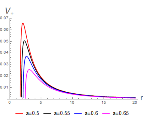
(a)

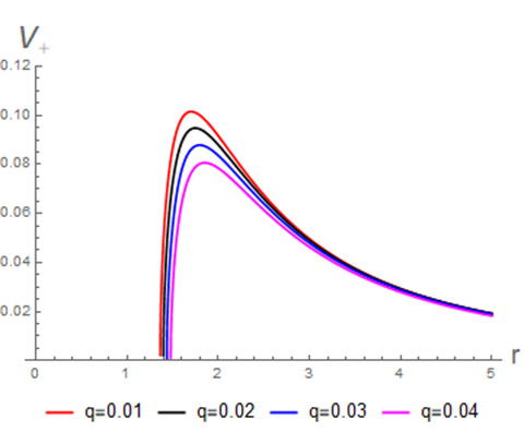
(b)

Figure 1: Shows the behaviour of $V_{+}$ (19) for various values of the string cloud parameter $a$ (left plot) and quintessence parameter $q$ (right plot). Here, $\lambda=1,k=0.2$ and $M=0.4$.

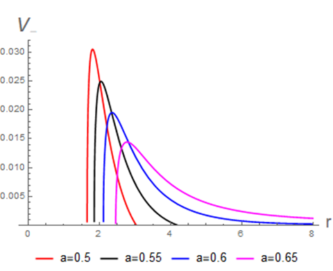
(a)

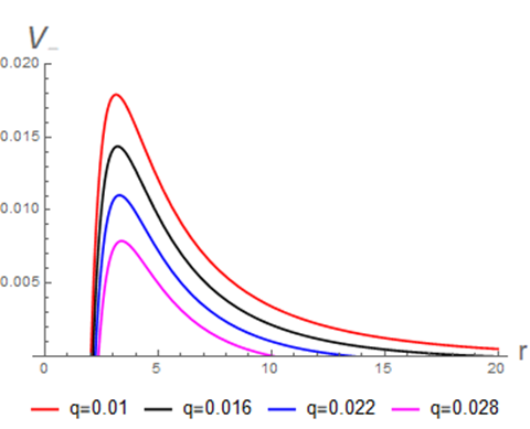
(b)

Figure 2: Shows the behaviour of $V_{-}$ (19) for various values of the string cloud parameter $a$ (left plot) and quintessence parameter $q$ (right plot). Here, $\lambda=1,k=0.2$ and $M=0.4$.

To elaborate the physical behavior of the potentials (19) in the physical region and to explore the effect of the quintessence parameters $q$ and the string cloud parameter $a$, we make two-dimensional plots of the potentials for the case $w_{q}=-2/3$ for which $f\left(r\right)=1-a-\frac{2M}{r}-qr$. Figures 1 and 2 represent the behavior of the potentials (19) for some specific values of the quintessence and the cloud of strings parameters. The figures show that the potentials become smaller with higher values of the quintessence and cloud of strings parameters. The figures indicate that as the quintessence and string cloud parameters increase, the potentials decline, so their main effect is to codify potentials and attenuate their peaks. As a result, we get a hint that when the potentials peaks diminish, the greybody factor will be higher.

II.2 Klein-Gordon equation

The massless scalar field $U(t,r,\theta,\phi)$ obeys the Klein-Gordon equation,

$$\frac{1}{\sqrt{-g}}\partial_{\mu}\sqrt{-g}g^{\mu\nu}\partial_{\nu}U(t,r,\theta,\phi)=0,$$ (22)

where $g$ is the determinant of the spacetime metric (1), so that $\sqrt{-g}=r^{2}\sin\theta$. Here, we are considering a static back ground, the field equation can be separated as $U=R\left(r\right)Y_{m}^{l}\left(\theta,\phi\right)\exp\left(-i\omega t\right)$, where $Y_{m}^{l}$ are the usual spherical harmonics. Then, the Klein-Gordon equation can be reduced to a one dimensional Schrödinger like equation as follows,

$$\frac{d^{2}U}{dr_{\ast}^{2}}+\left(\omega^{2}-V_{eff}\right)U=0,$$ (23)

where $r_{\ast}$ is the tortoise coordinate: $\frac{dr_{\ast}}{dr}=\frac{1}{f},$ and $V_{eff}$ is the effective potential given by

$$V_{eff}=f\left(\frac{\lambda}{r^{2}}+\frac{f^{\prime}}{r}\right).$$ (24)

where $\lambda=$ $-l(l+1)$, ($l$ is the angular quantum number).

The behaviour of the potential (24) is illustrated in Fig. 3. As one can see, the potential becomes lower when both quintessence parameter $q$ and string cloud parameters $a$ increase. Once again, this indicates that the greybody factor will increase as $q$ and $a$ increase.

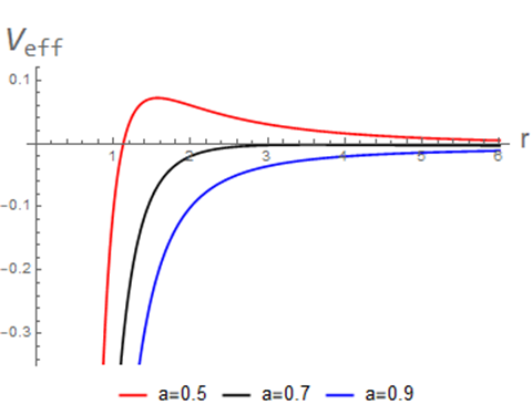
(a)

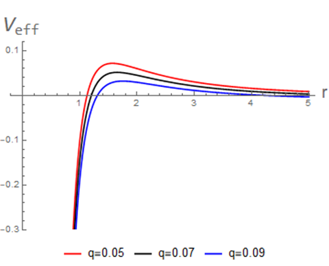
(b)

Figure 3: Shows the behaviour of $V_{eff}$ (24) for various values of the string cloud parameter $a$ (left plot) and quintessence parameter $q$ (right plot). Here, $\lambda=1$ and $M=0.2$.

III Greybody factor from SBH with string clouds and quintessence

III.1 Greybody factor of bosons

When quantum effects are considered, BHs can emit thermal radiation, called Hawking radiation. Greybody factor is one of the quantum quantities of a BH. It is the fraction of Hawking radiation that can reach spatial infinity. The Miller-Good transformation method [42-43] will be used to compute the greybody factor of bosons since the general semi-analytic bounds method yields a measureless greybody factor. Recall that, the Miller-Good transformation method, generates a general bound on quantum transmission probabilities. With this method, a particular transformation is applied to the Schrödinger equation (23) to modify the effective potential (24) and increase the probability that the Hawking quanta will be transmitted [44]. Hence, the transmission probability of bosons [14] is given by

$$\mathcal{T}\geq\sec h^{2}\left\{-\frac{1}{2\omega}\int_{r_{h}}^{+\infty}\left(\frac{f^{\prime}}{r}+\frac{\lambda}{r^{2}}\right)\frac{dr}{f}\right\}$$

which can be rewritten as

$$\mathcal{T}\geq\sec h^{2}\left\{\frac{1}{2\omega}\int_{r_{h}}^{+\infty}\left(2M+qr^{-3w_{q}}+\lambda r\right)\left(\frac{1}{r^{4}}\right)\frac{dr}{qr^{-3w_{q}-2}+\frac{2M}{r^{2}}-\frac{(1-a)}{r}}\right\}.$$ (25)

Here we obtain the gerybody factor for a specific value of EoS parameter for the quintessence $w_{q}$ $=-2/3$. Therefore, we consider the following asymptotic expansion

$$\frac{1}{qr^{-3w_{q}-2}+\frac{2M}{r^{2}}-\frac{(1-a)}{r}}\simeq\frac{1}{q}+\frac{1-a}{q^{2}r^{2}}+\frac{\left(1-a\right)^{2}-2Mq}{q^{3}r^{2}}+...,$$ (26)

as a result, we compute the greybody factor (25) as follows

$$\sigma_{l}\left(\omega\right)\equiv\mathcal{T}\geq\sec h^{2}\left\{\frac{1}{2\omega}\left[\frac{1}{r_{h}}-\frac{\lambda+a-1}{2qr_{h}^{2}}+\frac{1+a^{2}+a(\lambda-2)-\lambda-4Mq}{4q^{2}r_{h}^{3}}\right.\right.\\ \left.\left.\frac{2(a-1)Mq-\lambda(1-2a+a^{2}-2Mq)}{4q^{3}r_{h}^{4}}-\frac{2M(1-2a+a^{2}-2Mq)}{5q^{3}r_{h}^{5}}\right]\right\}.$$ (27)

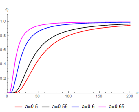
(a)

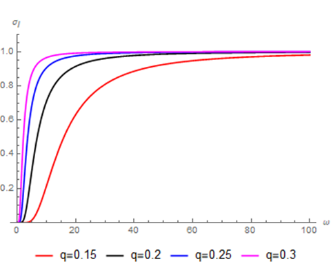
(b)

Figure 4: These plots show the bosonic greybody factor (27) for different values of the string cloud parameter $a$ (left plot) and quintessence parameter $q$ (right plot). Here, $\lambda=1,r=1$ and $M=0.4$.

The above computed equation (27) represents the bosonic greybody factor of SBH surrounded by quintessence and a cloud of strings, which is obtained by the Miller-Good transformation method. There is no doubt that the specific form of the greybody factor depends on some parameters that relate to the potential barrier. The greybody factor bound is actually determined by the shape of the potential. As in quantum theory, when the potential level increases, the amplitude of transmission decreases, and as a result the greybody factor bound decreases. The behavior of greybody factor (27) is depicted in Fig. 4. The plot shows that both the quintessence parameter $q$ and the string cloud parameter $a$ are significant for the greybody factors. A striking result is that $\sigma_{l}\left(\omega\right)$ increases with both $q$ and $a$ increasing.

III.2 Greybody factors of fermions

Here, we shall derive the fermionic gerybody factor of the neutrinos emitted from the SBH with string clouds and quintessence. The formula of the general semi-analytic bounds for greybody factors is  given by

$$\sigma_{l}\left(\omega\right)\geq\sec h^{2}\left(\int_{-\infty}^{+\infty}\wp dr_{\ast}\right),$$ (28)

where $\wp$ is the dimensionless greybody factor:

$$\wp=\frac{\sqrt{\left(h^{\prime}\right)^{2}+\left(\omega^{2}-V_{eff}-h^{2}\right)^{2}}}{2h},$$ (29)

in which $h^{\prime}$ implies the derivation with respect to $r$. By considering the conditions for $h$ (first, it must be positive and second $h\left(+\infty\right)=h\left(-\infty\right)=\omega$), we can simplify the function as [45]

$$\wp=\frac{1}{2\omega}V_{eff},$$ (30)

and using the tortoise coordinate as $\frac{dr_{\ast}}{dr}=\frac{1}{f\left(r\right)}$ then the greybody factor reads

$$\sigma_{l}\left(\omega\right)\geq\sec h^{2}\left(\frac{1}{2\omega}\int_{r_{h}}^{+\infty}V_{eff}\frac{dr}{f}\right).$$ (31)

To obtain analytical results from (31) we consider the case of EoS parameter for the quintessence $w_{q}=-1/3$ for which $f\left(r\right)=1-a-\frac{2M}{r}-q.$ Indeed, according to recent observational data of Planck Collaboration [46] the limit of EoS parameter is $-1.16<w_{q}<-0.92$ at the 95 % confidence level. This signifies a dark energy model of phantom type with $w_{q}$ less than $-1$. We are, however, primarily interested in computing the gerybody factor for a SBH with cloud of strings and quintessence. Thus, we limit our calculations to $-1\leq w_{q}\leq-1/3.$ We can now substitute the effective potential (19) into Eq. (31) to obtain

$$\sigma_{l}^{\pm}\left(\omega\right)\geq\sec h^{2}\frac{\lambda}{2\omega}\left(\frac{\lambda}{r_{h}}\pm\frac{1}{\sqrt{1-a-q}}\left(\frac{1-2a-2q}{r_{h}}+\frac{M\left(a+q-2\right)}{2\left(1-a-q\right)r_{h}^{2}}\right.\right.$$

$$\left.-\frac{M^{2}}{2\left(1-a-q\right)^{2}r_{h}^{3}}-\frac{M^{3}\left(a+q+4\right)}{8\left(1-a-q\right)^{3}r_{h}^{4}}+\frac{M^{4}\left(5-2a-2q\right)}{8\left(1-a-q\right)^{4}r_{h}^{5}}\right),$$ (32)

in which $\sigma_{l}^{+}(w)$ and $\sigma_{l}^{-}(w)$ stand for the greybody factors of the spin-up and spin-down fermions, respectively.

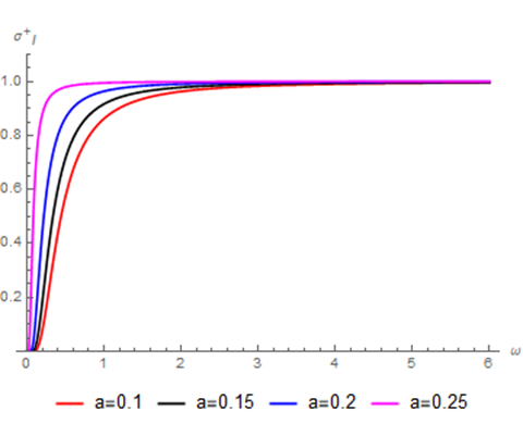
(a)

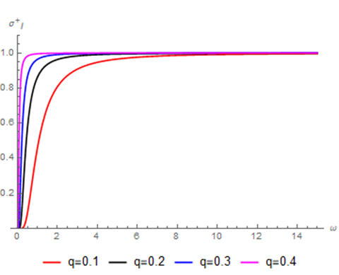
(b)

Figure 5: These plots show the fermionic greybody factor spin (+1/2) (32) for different values of the string cloud parameter $a$ (left plot) and quintessence parameter $q$ (right plot). Here, $\lambda=1,r=1$ and $M=0.5$.

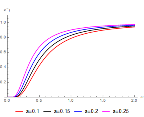
(a)

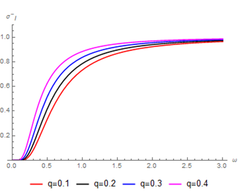
(b)

Figure 6: These plots show the fermionic greybody factor spin (-1/2) (32) for different values of the string cloud parameter $a$ (left plot) and quintessence parameter $q$ (right plot). Here, $\lambda=1,r=1$ and $M=0.5$.

Figures 5 and 6 demonstrate the behavior of spin (+1/2) and spin (-1/2) under the influence of both the quintessence parameter and string cloud parameter. According to 5 and 6 the greybody factors increase as $q$ and $a$ increase as with bosons.

IV Conclusion

In this paper, we have studied the scalar and spinor perturbations as well as the greybody radiation in the spacetime of SBH surrounded by quintessence and a cloud of strings. We examine the Klein-Gordon and Dirac equations, respectively, for scalar and spinor perturbations. Using the massless uncharged scalar/spinor field emitted from the SBH with quintessence and a cloud of strings as Hawking radiation, a Schrödinger-like equation with effective potentials for the radial part of the solution is obtained. Both quintessence $\left(q\right)$ and string cloud $\left(a\right)$ parameters contribute to the effective potentials. To understand the physical interpretations and the effect of $q$ and $a$ on the potentials, we plot the potentials for a variety of parameter values. It is found that the height of the potentials becomes lower as both $q$ and $a$ increase. Consequently, we get a clue that the greybody factor bound will rise as the potential peaks diminish.

In the analysis of the thermal radiation of the SBH surrounded by quintessence and a cloud of strings, we have utilized the Miller-Good transformation and the general semi-analytic bounds to obtain the greybody factors of bosons and fermions, respectively. So, we have shown the effect of $q$ and $a$ parameters on the Hawking radiation, which can be detected by observers at spatial infinity. We also supported our results with graphics. It is found that the greybody factors bound increase as both $q$ and $a$ increase. Thus, the lower the potential, the easier it is for the waves to be transmitted and therefore, the higher the bound of the greybody factors. This is in accordance with quantum mechanics.

Data availability statement:
My manuscript has no associated data.

References

[1] A.G. Riess et al., Observational evidence from supernovae for an accelerating universe and a cosmological constant. Astron. J. 116, 1009–1038 (1998)

[2] S. Perlmutter et al., Measurements of omega and lambda from 42 high redshift supernovae. Astrophys. J. 517, 565–586 (1999)

[3] Steinhardt, P.J., Wang, L., Zlatev, I.: Phys. Rev. D 59, 123504 (1999)

[4] Wang, L., Caldwell, R., Ostriker, J., Steinhardt, P.J.: Astron. J. 530, 17 (2000).

[5] Tsujikawa, S.: Class. Quantum Gravity 30, 214003 (2013).

[6] M. Liu, J. Lu and Y. Gui, Eur. Phys. Jour. C 59 (2009) 107.

[7] V. Kiselev, Class. Quantum Gravity 20 (2003) 1187.

[8] B. Toshmatov, Z. Stuchlík, B. Ahmedov, Eur. Phys. J. Plus 132 (2017).

[9] S.G. Ghosh, Eur. Phys. J. C 76 (2016) 1

[10] S. Fernando, Gen. Relativ. Gravit. 44, 1857 (2012)

[11] K. Ghaderi, Astrophys. Space Sci. 362, 218 (2017).

[12] F. Cicciarella, M. Pieroni, JCAP 1708 (2017).

[13] M. Saleh, B. Thomas, T. Kofane, Eur. Phys. J. C 78:325 (2018).

[14] A. Al-Badawi, S. Kanzi, I. Sakalli, Eur. Phys. J. Plus 135, 219 (2020)

[15] I. AliKhan, A. SultanKhan, S. Islam, Int. J. Mod. Phys. A 35(23), 2050130 (2020).

[16] R. Saadati, F. Shojai, Phys. Rev. D 100, 104041 (2019) 17.

[17] I. Hussaina, S. Alib, Eur. Phys. J. Plus 131, 275 (2016).

[18] K. Ghaderi, B. Malakolkalami, Astrophys. Space Sci. 361 (2016) 161.

[19] P.S. Letelier, Clouds of strings in general relativity. Phys. Rev. D 20, 1294–1302 (1979).

[20] J. Stachel, Phys. Rev. D 21 (1980) 2171.

[21] H. H. Soleng, Gen. Relativ. Gravit. 27 (1995) 367.

[22] L. L. Smalley and J. P. Krisch, Class. Quantum Gravity 14 (1997) 3501.

[23] M. Batool, I. Hussain, Int. J. Mod. Phys. D 26(05), 1741005 (2017).

[24] Efferson de M. Toledo and V. B. Bezerra, Eur. Phys. J. C 78 534 (2018).

[25] Sushant G. Ghosh, Sunil D. Maharaj, Dharmanand Baboolal and Tae-Hun Lee, Eur. Phys. J. C 78 90 (2018).

[26] Estanislav Herscovich and Martin G. Richarte, Phys. Lett. B 689 (2010) 192.

[27] Tae-Hun Lee, Dharmanand Baboolal and Sushant G. Ghosh, Eur. Phys. J. C 75 (2015) 297

[28] Bouetou Bouetou Thomas, Mahamat Saleh and Timoleon Crepin Kofane, Gen. Rel. Grav. 44 (2012) 2181.

[29] Y.S. Myung, H.W. Lee, Classical Quantum Gravity 20 (2003) 3533.

[30] T. Harmark, J. Natario, R. Schiappa, Adv. Theor. Math. Phys. 14 (2010) 727.

[31] I. Sakalli, O.A. Aslan, Astropart. Phys. 74 (2016) 73.

[32] H. Gursel, I. Sakalli, Adv. High Energy Phys. 2018 (2018) 8504894.

[33] A. Al-Badawi, I. Sakalli, S. Kanzi, Ann. Phys. 412, 168026 (2020).

[34] H. Gursel, I. Sakalli, Eur. Phys. J. C 80, 234 (2020).

[35] S. Kanzi, S.H.Mazharimousavi, I. Sakalli, Ann. Phys. 422, 168301 (2020).

[36] S. Kanzi, I. Sakallı, Eur. Phys. J. C 81, 501 (2021).

[37] J.M. Toledoa, V.B. Bezerra, Eur. Phys. J.C 78, 534 (2018).

[38] J.M. Toledo, V.B. Bezerra, Int. J. Mod. Phys. D 28, 1950023 (2019).

[39] M.M. DiaseCosta, J.M. Toledo, V.B. Bezerra, Int. J. Mod. Phys. D 28, 1950074 (2019)

[40] ] S. Chandrasekhar, The Mathematical Theory of Black Holes, Clarendon, London, 1983.

[41] E.T. Newman, R. Penrose, J. Math. Phys. 3 (1962) 566.

[42] P. Boonserm, M. Visser, J. Phys. A Math. Theor. 42, 045301 (2009).

[43] S. C. Miller and R. H. Good, Phys. Rev. 91 (1953) 174–179.

[44] R.M. Wald, General Relativity (The University of Chicago Press, Chicago and London, 1984).

[45] Y.G. Miao, Z.M. Xu, Phys. Lett. B 772 (2017) 542.

[46] Planck Collaboration:. Astron. Astrophys. 571, A16 (2014).