Analysis of a new type of fractional linear multistep method of order two with improved stability

Abstract

We present and investigate a new type of implicit fractional linear multistep method of order two for fractional initial value problems. The method is obtained from the second order super convergence of the Grünwald-Letnikov approximation of the fractional derivative at a non-integer shift point. The proposed method is of order two consistency and coincides with the backward difference method of order two for classical initial value problems when the order of the derivative is one. The weight coefficients of the proposed method are obtained from the Grünwald weights and hence computationally efficient compared with that of the fractional backward difference formula of order two. The stability properties are analyzed and shown that the stability region of the method is larger than that of the fractional Adams-Moulton method of order two and the fractional trapezoidal method. Numerical result and illustrations are presented to justify the analytical theories.

Keywords: Fractional derivative, Grünwald approximation, super convergence, Generating functions, fractional Adams-Moulton methods, stability regions

Subject Classification: 26A33, 34A08, 34D20, 65L05, 65L20

1 Introduction

Consider the fractional initial value problem (FIVP)

$$\;{}^{C}_{t_{0}}D^{\beta}_{t}y(t) =f(t,y(t)),\quad t\geq t_{0},\quad 0<\beta\leq 1,$$ (1a)

$$y(t_{0}) =y_{0},$$ (1b)

where $\;{}^{C}_{t_{0}}D^{\beta}_{t}$ is the left Caputo fractional derivative operator defined in Section 2, $f(t,y)$ is a source function satisfying Lipschitz condition in the second argument $y$ guaranteeing a unique solution to the problem [4].

Fractional calculus, despite its long history, have only recently gained places in science, engineering, artificial intelligence and many other fields.

Many numerical methods have been developed in the recent past for solving (1) approximately. We are interested in the numerical methods of type commonly known as the fractional linear multistep methods (FLMM).

The basic numerical method of FLMM type of order one for (1) is obtained from the Grünwald-Letnikov form for the fractional derivative [22, 21]. The weight coefficients for this basic FLMM are the Grünwald weights obtained from the series of the generating function $(1-z)^{\beta}$.

Lubich [12] introduced a set of higher order FLMMs as convolution quadratures for the Volterra integral equation (VIE) obtained by reformulating (1) (See also eg. [4]). The quadrature coefficients are obtained from the fractional order power of the rational polynomial obtained from the generating polynomials of linear multistep method (LMM) for classical initial value problems (IVPs). As a particular subfamily of these FLMMs, the fractional backward difference formulas (FBDFs) were also proposed by Lubich in [13]. Another particular form of FLMM type is the fractional trapezoidal method of order 2.

Several authors have utilized these formulations to construct variations of the FLMMs, see eg. [5] and the references therein. Galeone and Garrappa [6] studied some implicit FLMMs generalizing the Adams-Moulton methods for classical IVPs. Galeone and Garrappa [7] and Garrappa [8] have investigated a set of explicit FLMMs generalizing the Adams-Bashforth methods.

In [17], the authors constructed a new type of FLMM of order 2 that does not fall under the above mentioned subfamilies of FLMMs and presented an extended abstract in [18].

In this paper, we analyse the method for computation and stability, and present an algorithm. We also compare the method with other known FLMMs of order 2 and show that the presented method outweighs the other methods in stability and/or computational efficiency.

This paper is organized as follows. In Section 2, the preliminaries and previous relevant works are summarized. In Section 3, the new FLMM of order 2 is introduced along with a computational algorithm. Numerical examples for testing the method are given in Section 4. In Section 5, the stability of the method is analysed. In Sections 6, the new method is compared with other FLMMs and Section 7 draws some conclusions.

2 Preliminaries

The Riemann-Liouville fractional integral of order $\beta>0$ of a function $f(t)$ in an interval domain $[t_{0},T)$ ( $T$ can also be infinity) is defined as

$$J_{t}^{\beta}f(t)=\frac{1}{\Gamma(\beta)}\int_{t_{0}}^{t}(t-\tau)^{\beta-1}f(\tau)d\tau,$$ (2)

where $\Gamma(\cdot)$ denotes the Euler-Gamma function.

For a sufficiently smooth function $y(t)$ defined for $t\geq t_{0}$, the left Riemann-Liouville (RL) fractional derivative of order $\beta>0$ is defined by (see eg. [22])

$$\;^{RL}_{t_{0}}D^{\beta}_{t}y(t)=\frac{1}{\Gamma(m-\beta)}\frac{d^{m}}{dx^{m}}\int_{t_{0}}^{t}\frac{y(\tau)}{(t-\tau)^{\beta-m+1}}d\tau,\quad m-1<\beta\leq m,$$ (3)

where $m=\lceil\beta\rceil$ – the smallest integer larger than or equal to $\beta$.

The left Caputo fractional derivative of order $\beta>0$ is defined as

$$\;^{C}_{t_{0}}D^{\beta}_{t}y(t)=J^{m-\beta}_{t}y^{(m)}(t)=\frac{1}{\Gamma(m-\beta)}\int_{t_{0}}^{t}\frac{y^{(m)}(\tau)}{(t-\tau)^{\beta-m+1}}d\tau,\quad m-1<\beta\leq m,$$ (4)

where $y^{(m)}$ is the $m$-th derivative of $y$.

Often, for practical reasons, the integer ceiling $m$ of the fractional order $\beta$ is considered to be one or two. In this paper, we investigate (1) for the case $0<\beta\leq 1$ when $m=1$.

In addition to the above two definitions, the Grünwald-Letnikov(GL) definition is useful for numerical approximations of fractional derivatives.

$$\,^{GL}_{t_{0}}D^{\beta}_{t}y(t)=\lim_{h\rightarrow 0}\frac{1}{h^{\beta}}\sum_{k=0}^{\infty}g_{k}^{(\beta)}y(t-kh),$$ (5)

where $g_{k}^{(\beta)}=(-1)^{k}\frac{\Gamma(\beta+1)}{\Gamma(\beta-k+1)k!}$ are the Grünwald weights and are the coefficients of the series expansion of the Grünwald generating function

$$\omega_{1}(z)=(1-z)^{\beta}=\sum_{k=0}^{\infty}g_{k}^{(\beta)}z^{k}.$$ (6)

The coefficients can be successively computed by the recurrence relation

$$g_{0}^{(\beta)}=1,\qquad g_{k}^{(\beta)}=\left(1-\frac{\beta+1}{k}\right)g_{k-1}^{(\beta)},\quad k=1,2,...\;.$$

For theoretical purposes, the function $y(t)$ has been zero extended for $t<t_{0}$ and hence the infinite summation in the GL definition (5). Practically, the upper limit of the sum is $n=[(t-t_{0})/h]$, where $[x]$ denotes the integer part of $x$.

The three definitions in (3)–(5) are equivalent under homogeneous derivative conditions at the initial point $t_{0}$ [22].

2.1 Approximation of fractional integrals and derivatives

Numerical approximation of the fractional integral (2) is commonly considered via convolution quadrature formulas of the form

$$J_{h}^{\beta}f(t)=h^{\beta}\sum_{k=0}^{n}\omega_{k}f_{n-k},$$ (7)

where the interval $[t_{0},t]$ is discretized by the points set $\{t_{0},t_{1},...,t_{n}\}$ with $t_{k}=t_{0}+kh,f_{k}=f(t_{k}),$ for $k=0,1,...,n,$ and $h=(t-t_{0})/n$. The weights $\omega_{k}$ are from the quadrature rule applied.

For numerical approximation of the fractional derivative, the GL definition is commonly used by dropping the limit in (5) resulting in the Grünwald approximation (GA) for a fixed step $h$ [21].

$$\delta_{h}^{\beta}y(t):=\frac{1}{h^{\beta}}\sum_{k=0}^{\infty}g_{k}^{(\beta)}y(t-kh).$$ (8)

It is known that the GA is of order one [15, 16].

$$\delta_{h}^{\beta}y(t):=\,^{GL}_{t_{0}}D^{\beta}_{t}y(t)+O(h).$$ (9)

A more general Grünwald type approximation is given by the shifted Grunwald approximation (SGA) [15].

$$\delta_{h,r}^{\beta}y(t)=\frac{1}{h^{\beta}}\sum_{k=0}^{\infty}g_{k}^{(\beta)}y(t-(k-r)h),$$ (10)

where $r$ is the shift parameter.

For an integer shift $r$, the SGA is also of first order approximation [15].

$$\delta_{h,r}^{\beta}y(t)=\,^{GL}_{t_{0}}D^{\beta}_{t}y(t)+O(h),\quad r\in\mathbb{Z}.$$

However, it is observed that the SGA gives a second order approximation at a non-integer shift $r=\beta/2$ displaying super convergence [16].

$$\delta_{h,\beta/2}^{\beta}y(t)=\,^{GL}_{t_{0}}D^{\beta}_{t}y(t)+O(h^{2}).$$ (11)

Some higher order Grünwald type approximations with shifts were presented in [10] with the weight coefficients obtained from some generating functions given in an explicit form according to the order and shift requirements.

2.2 Fractional initial value problem

For $m-1<\beta\leq m$, the general form of a FIVP is given by

$$\;{}^{C}_{t_{0}}D^{\beta}_{t}\bar{y}(t) =\bar{f}(t,\bar{y}(t)),\quad t\geq t_{0},\quad m-1<\beta\leq m,$$ (12a)

$$\bar{y}^{(k)}(t_{0}) =y_{0}^{(k)},\quad k=0,1,...,m-1.$$ (12b)

Without loss of generality, one may consider the FIVP with homogeneous initial conditions at the origin ($t_{0}=0$):

$$\,{}^{RL}_{\;\;0}D^{\beta}_{t}y(t) = f(t,y(t)),\quad t\geq 0,\quad m-1<\beta\leq m,$$ (13a)

$$y^{(k)}(0) = 0,\quad k=0,1,...,m-1,$$ (13b)

because $y(t)$ is a solution of (13) if and only if

$$\bar{y}(t)=y(t-t_{0})+T_{m-1}(t-t_{0})$$ (14)

is the solution of (12), where

$$T_{m-1}(t)=\sum_{k=0}^{m-1}\frac{t^{k}}{k!}y_{0}^{(k)},\quad f(t,y)=\bar{f}(t+t_{0},\bar{y}(t+t_{0})).$$

For $0<\beta\leq 1$, we have $T_{0}(t)=y_{0}$ and $f(t,y)=\bar{f}(t+t_{0},y(t+t_{0})+y_{0})$.

The problem (13) can be equivalently expressed by the VIE of second kind [4]

$$y(t)=\frac{1}{\Gamma(\beta)}\int_{0}^{t}(t-\eta)^{\beta-1}f(\eta,y(\eta))d\eta.$$ (15)

2.3 Fractional linear multistep methods

Among the several numerical methods to solve (13) and thus (15), we list the numerical methods that fall under the category of FLMM.

The Grünwald-Letnikov method: The fundamental and widely investigated numerical approximation scheme for the FIVP (13) is the Grünwald-Letnikov method (also called fractional backward Euler method) obtained by replacing the fractional derivative operator in (13a) by its GA operator $\delta^{\beta}_{h}$ in (8) with (9) [22].

$$\frac{1}{h^{\beta}}\sum_{k=0}^{\infty}g_{k}^{(\beta)}y(t-kh)=f(t,y)+O(h).$$ (16)

By choosing the discretization step $h$ appropriately to align the discrete points $t-kh$ with the end points of the problem domain $[0,T]$ and assuming zero extension for the unknown function $y(t)$ for $t<0$, the infinite sum in (16) is reduced to a finite sum. Dropping the first order error term, choosing $h=T/N,N\in\mathbb{N}$ and denoting

$$t_{n}=nh,\quad y_{n}\approx y(t_{n})\quad\text{ and }\quad f_{n}=f(t_{n},y_{n}),$$ (17)

equation (16) gives the GL scheme

$$\sum_{k=0}^{n}g_{k}^{(\beta)}y_{n-k}=h^{\beta}f_{n},\quad n=1,2,...,N.$$ (18)

The FIVP can also be approximated via its VIE form (15) by simply replacing the integral by its approximation (7). Some approximations in this line are the product integration methods [23, 3, 14].

Lubich [13] presented and studied numerical approximation methods for the VIE (15) in the form

$$y_{n}=h^{\beta}\sum_{k=0}^{n}\omega_{k}f_{n-k},\quad n=1,2,...$$ (19)

with weights $\omega_{k}$ as the coefficients of the series expansion of the generating function

$$\omega(\xi)=\left(\frac{\sigma(1/\xi)}{\rho(1/\xi)}\right)^{\beta},$$

where $(\rho,\sigma)$ is a pair of generating polynomials of a LMM of a prescribed order for classical IVP. However, Lubich observed and showed that for approximations of order more than one, the intended order $p$ is achieved only for a certain class of functions, specifically for functions of the form $y(t)=t^{\alpha-1}g(t),\alpha\geq p$, where $g(t)$ is analytic. However, for $\alpha<p,$ the order is reduced to $O(h^{\alpha})$ only. To remedy this order reduction, an additional sum is introduced in (7) to have the approximation scheme

$$y_{n}={h^{\beta}}\sum_{k=0}^{s}w_{n,k}f_{k}+{h^{\beta}}\sum_{k=0}^{n}w_{k}f_{n-k}.$$ (20)

Here, the starting weights $w_{n,k}$ are to compensate the reduced order of convergence.

Another way to approximate the FIVP (13) is to replace the fractional derivative by its approximation in the form (8) with general weights $w_{k}$ as

$$\Omega_{h}^{\beta}y(t):=\frac{1}{h^{\beta}}\sum_{k=0}^{\infty}w_{k}y(t-kh),$$ (21)

where the weights $w_{k}$ are chosen for a desired order of approximation. Thus, Grunwald type approximation schemes for the FIVP have the form expressed in conformance with the classical LMM form as

$$\sum_{k=0}^{n}w_{k}y_{n-k}=h^{\beta}f_{n},\quad n=1,2,...\;.$$ (22)

Remark 1: Note that, analogous to the case of FLMM for VIE, the FLMM for FIVP also displays the order reduction for the class of functions mentioned for the FLMM for VIE. Therefore, an adjusting sum with some starting weights is added to remedy this situation. We also point out, however, that this additional sum does not affect the convergence and stability of the underlying FLMM. Besides, including this sum in the computation of solution, though it rectifies the order, brings additional difficulties in the implementation such as (i) the number of starting weights vary depending on the fractional order $\beta$, (ii) computing the starting weights at every iterations, (iii) the system to solve for the starting weights is highly ill conditions, etc.

It can be shown that the approximation schemes (19) and (22) are equivalent (see [6] and the references therein) and the generating functions $\omega(\xi)$ and $\delta(\xi)$ of the weight coefficients $\omega_{k}$ and $w_{k}$ in (19) and (22) respectively can be shown to have the relation $\delta(\xi)=(\omega(\xi))^{-1}$. Thus, the weights $w_{k}$ in (19) can be chosen as the coefficients of the series expansion of the generating function

$$\delta(\xi)=\left(\frac{\rho(1/\xi)}{\sigma(1/\xi)}\right)^{\beta}.$$ (23)

Lubich [13] also presented some subclasses of FLMMs for VIE with generating functions of general form $(r_{1}(\xi)^{\beta}r_{2}(\xi)$, where $r_{1}(\xi),r_{2}(\xi)$ are rational polynomials. Analogously, the FLMMs for FIVP can also be considered with the generating functions of the form

$$\delta(\xi)=\left(\frac{a(\xi)}{b(\xi)}\right)^{\beta}\frac{p(\xi)}{q(\xi)},$$ (24)

where $a,b,p$ and $q$ are polynomials.

2.4 Stability regions for the FLMM

The following definitions are fundamental for the analysis of stability of a FLMM.

Definition 1.

[Stability] Let $y_{n}$ be a solution of a recurrence relation with initial data vector ${\bf y}_{0}$.

1. $y_{n}$ is stable if for any perturbation $\delta{\bf y}_{0}$ in ${\bf y}_{0}$, the resulting changes $\delta y_{n}$ in $y_{n}$ are uniformly bounded for all $n\in\mathbb{N}$.

2. The solution is asymptotically stable if, moreover, $\delta y_{n}\rightarrow 0$ as $n\rightarrow\infty$.

The stability region for FLMM is given by

$$S_{\beta}=\{\lambda h^{\beta}\in\mathbb{C}\setminus\{0\}:y_{n}\rightarrow 0\text{ as }n\rightarrow\infty\},$$

where $\lambda$ is a complex parameter of the stability test problem  ${}^{C}D^{\beta}y(t)=\lambda y(t),y(0)=y_{0}$.

The generating function for an FLMM directly gives the stability region for the method.

Theorem 1.

[13] The stability region of an FLMM with generating function $\delta(\xi)$ is given by

$$S=\{\delta(\xi):|\xi|>1\},$$ (25)

We list the subfamilies of the FLMMs found in the literature.

1. Fractional trapezoidal method: The fractional trapezoidal method of order 2 (FT2) obtained from the trapezoidal rule for the ODE has the generating function[13]

   $$\delta_{FT2}(\xi)=\left(2\frac{1-\xi}{1+\xi}\right)^{\beta}.$$

   It is the only method known so far in the form $\delta(\xi)=\left(\frac{a(\xi)}{b(\xi)}\right)^{\beta}$ with $b(\xi)\neq 1,p(\xi)=q(\xi)=1$ in (24).

2. Fractional backward difference formula: The fractional backward difference formula (FBDF) obtained from the BDF for classical IVP has the generating functions of the form $\delta(\xi)=(a(\xi))^{\beta}$.

   For orders $1\leq m\leq 6$, a set of 6 FDBF$m$ methods have been obtained with polynomials corresponding to the generating polynomials of the BDF of order $m$ given by $a(\xi)=\sum_{k=1}^{m}\frac{1}{k}(1-\xi)^{k}$.

3. Fractional Adams methods: The fractional Adams methods have the generating functions of the form $\delta(\xi)=\frac{(a(\xi)^{\beta}}{q(\xi)}$, where the polynomial $a(\xi)$ is one of the polynomials in FBDF methods and $q(\xi)$ is determined to have a specified order of consistency for the method. Often, $a(\xi)=1-\xi$ [5, 6, 7, 8]. However, other polynomials in the FBDF have also appeared in the literature [2, 11].

   When $q_{0}=0$, the method is explicit and is called fractional Adams-Bashforth methods (FABs) [7, 8]. $q_{0}\neq 0$ gives implicit methods and are called fractional Adams-Moulton methods (FAMs).

4. Rational approximation: In [1], a classical LMM type of approximation is proposed to obtain a class of FLMMs by rational approximations of the FBDF generating functions in the form $\delta(\xi)=\frac{p(\xi)}{q(\xi)}$.

The order of consistency of a FLMM can also be determined from its generating function.

Theorem 2.

[20, 19, 10]. The order of an FLMM with generating function $\delta(\xi)$ is $p$ if and only if

$$\frac{1}{x^{\beta}}\delta(e^{-x})=1+O(x^{p}).$$ (26)

Moreover, the approximation corresponding to $\delta(\xi)$ satisfies, with $D_{t}^{\beta}$ denoting the RL fractional derivative,

$$\delta_{h}^{\beta}y(t)=D_{t}^{\beta}y(t)+h^{p}a_{p}(\beta)D_{t}^{\beta+p}y(t)+h^{p+1}a_{p+1}(\beta)D_{t}^{\beta+p+1}y(t)+...,$$

where $y(t)$ is assumed to be sufficiently smooth.

3 A new fractional linear multistep method

We present the main result of constructing a new FLMM of order 2.

The fractional derivative of the FIVP (13) is replaced by the approximation (11) with super convergence of order 2. This gives at $t=t_{n}$,

$$\delta_{h,\beta/2}^{\beta}y(t_{n})=\frac{1}{h^{\beta}}\sum_{k=0}^{\infty}g_{k}^{(\beta)}y(t_{n}-(k-\beta/2)h)=f(t_{n},y(t_{n}))+O(h^{2}).$$ (27)

Since $k-\beta/2$ is not integer for $0<\beta\leq 1$, the point $t_{n}-(k-\beta/2)h=:t_{n-k+\beta/2}$ is not aligned with the discrete points of the computational domain $\{t_{m},m=0,1,...,N\}$. Replace it with an order 2 approximation with points $t_{n-k}$ and $t_{n-k-1}$ in the computational domain given by

$$y\left(t_{n-k+\beta/2}\right)=\left(1+\beta/2\right)y(t_{n}-kh)-(\beta/2)y(t_{n}-(k-1)h)+O(h^{2}).$$ (28)

With the notations in (17), we obtain the new implicit FLMM approximation scheme

$$\sum_{k=0}^{\infty}g_{k}^{(\beta)}\left[\left(1+\frac{\beta}{2}\right)y_{n-k}-\frac{\beta}{2}y_{n-k-1}\right]=h^{\beta}f_{n},\quad n=1,2,\cdots.$$ (29)

The coefficients in the new FLMM (29) are linear expressions of the Grünwald weights $g_{k}^{(\beta)}$ and thus does not involve any extra computations.

For the order of the method, we have the following:

Theorem 3.

The new FLMM in (29) is consistent with order 2.

Proof.

Immediately follows from (11), (27) and (28). ∎

Theorem 4.

The generating function of the new implicit FLMM is given by

$$\delta(\xi)=(1-\xi)^{\beta}p(\xi),$$ (30)

where $p(\xi)=\left(1+\frac{\beta}{2}\right)-\frac{\beta}{2}\xi.$ Moreover, the generating function satisfies

$$\frac{1}{x^{\beta}}\delta(e^{-x})=1+O(x^{2})$$

confirming order 2 consistency.

Proof.

The sum on the left side of (29) is manipulated with $p_{0}=1+\beta/2,\quad p_{1}=-\beta/2$ as follows:

$$\sum_{k=0}^{\infty}g_{k}^{(\beta)}\left(p_{0}y_{n-k}+p_{1}y_{n-k-1}\right) =p_{0}\sum_{k=0}^{\infty}g_{k}^{(\beta)}y_{n-k}+p_{1}\sum_{k=0}^{\infty}g_{k}^{(\beta)}y_{n-k-1}$$

$$=p_{0}\sum_{k=0}^{\infty}g_{k}^{(\beta)}y_{n-k}+p_{1}\sum_{k=1}^{\infty}g_{k-1}^{(\beta)}y_{n-k}=\sum_{k=0}^{\infty}\left(p_{0}g_{k}^{(\beta)}+p_{1}g_{k-1}^{(\beta)}\right)y_{n-k},$$ (31)

where we have set $g_{-1}^{(\beta)}=0$. The weights

$$w_{k}=p_{0}g_{k}^{(\beta)}+p_{1}g_{k-1}^{(\beta)},\quad k=0,1,...\;.$$ (32)

are the coefficients of the generating function

$$\delta(\xi)=p_{0}(1-\xi)^{\beta}+p_{1}\xi(1-\xi)^{\beta}=(1-\xi)^{\beta}(p_{0}+p_{1}\xi).$$

Moreover, we have

$$\frac{1}{x^{\beta}}\delta(e^{-x})=1-\frac{\beta(3\beta+5)}{24}x^{2}+O(x^{3}).$$

which completes the proof. ∎

Remark 2: When $\alpha=1$, the new FLMM coincides with the BDF2 method $(\rho,\sigma)$ of order 2 for the classical IVP with generating polynomials $\rho(\xi)=\frac{3}{2}-2\xi+\frac{1}{2}\xi^{2}$ and $\sigma(\xi)=1$.

Remark 3: The notion of super convergence and nodal alignment have been applied for space fractional diffusion equations in [16] and [24]. To the knowledge of the authors, super convergence of Grünwald approximation for time fractional differential equations has not appeared before in the literature.

3.1 Implementation

Here, we give two algorithms to compute the approximate solutions for the FIVP for linear and non-linear cases using the new FLMM .

As the starting weights do not affect the convergence and stability, we exclude the starting sum in the algorithms (see also Remark 1). For details of implementing the starting sum, the reader is directed to [9].

For brevity of notations, the convolution of two vectors ${\bf a,b}$ of size $n+1$ is denoted by ${\bf a*b}=\sum_{k=0}^{n}a_{k}b_{n-k}$. For a sequence ${\bf a}$, the vector slice $[a(i),a(i+1),\ldots,a(j)]$ is denoted by ${\bf a}_{i,j}$.

We reformulate the new FLMM scheme (29) with (31) and (32) as

$$\sum_{k=0}^{n}w_{k}y_{n-k}={\bf w}_{0,n}*{\bf y}_{0,n}=w_{0}y_{n}+{\bf w}_{1,n}*{\bf y}_{0,n-1}=\lambda h^{\beta}f_{n}.$$ (33)

In the case of linear FIVP, we have $f(t,y)=\lambda y(t)+s(t)$ for some constant $\lambda$ and function $s(t)$.

We write the scheme (33) for this case, with $s_{n}=s(t_{n})$, as

$$w_{0}y_{n}+{\bf w}_{1,n}*{\bf y}_{0,n-1}=h^{\beta}(\lambda y_{n}+s_{n})\Rightarrow y_{n}=\frac{1}{w_{0}-\lambda h^{\beta}}\left[h^{\beta}s_{n}-{\bf w}_{1,n}*{\bf\bar{y}}_{0,n-1}\right],\quad n=1,2,...\;.$$

Hence, the algorithm for the linear FIVP is devised as

Algorithm 1 [For linear FIVP]

1. Input $\lambda,s(t)$ , $y_{0}$ and $t_{0},h,N$.

2. Compute sequence ${\bf w}_{0,N}$.

3. For $n=1,2,\ldots,N$, Compute $y_{n}=\frac{1}{w_{0}-\lambda h^{\beta}}\left[h^{\beta}s_{n}-{\bf w}_{1,n}*{\bf\bar{y}}_{0,n-1}\right]$.

For non-linear FIVP, the non-linear equation (33) in $y_{n}$ needs to be solved for the unknown $y_{n}$. The Newton-Raphson method is used to numerically solve this with an initial seed $y_{n,0}=y_{n-1}$. Thus, the following algorithm results for non-linear FIVP.

Algorithm 2 [For non-linear FIVP]

1. Input $f(t,y),f_{y}(t,y)$ , $y_{0}$

2. For $n=1,2,\ldots,N$,

3. $c_{n}={\bf w}_{1,n}*{\bf\bar{y}}_{0,n-1}$

4. Set $y_{n,0}=y_{n-1}$.

5. For $k=1,2,\ldots,$

6. Compute $F_{k-1}=w_{0}y_{n,k-1}-h^{\beta}f(t_{n},y_{n,k-1})+c_{n}$.

7. Compute $JF_{k-1}=w_{0}-h^{\beta}f_{y}(t_{n},y_{n,k-1})$

8. Compute $y_{n,k}=y_{n,k-1}-\frac{F_{k-1}}{JF_{k-1}}.$

9. Until convergence at $k=K$.

10. Set $y_{n}=y_{n,K}$.

4 Numerical Tests

We used the new FLMM to compute approximate solutions of the non-linear FIVP

$$D^{\beta}y(t) =f(t,y),\quad 0\leq t\leq 1,0<\beta\leq 1,$$

$$y(0) =0.$$

where

$$f(t,y)=\frac{\Gamma(2\beta+5)}{\Gamma(\beta+5)}t^{\beta+4}-\frac{240}{\Gamma(6-\beta)}t^{(5-\beta)}+(t^{2\beta+4}-2t^{5})^{2}-y(t)^{2}.$$

The exact solution of the problems is given by $y(t)=t^{2\beta+4}-2t^{5}$.

The problem is solved with fractional orders $\beta=0.4,0.6,0.8$ and $1.0$. The computational domain of the problem is $\{t_{n}=n/M,n=0,1,\cdots,M\}$ and step size $h=1/M$, where $M$ is the number of subintervals of the problem domain $[0,1]$. The problem was computed for $M=2^{j},j=3,4,...,12$.

The computational order of the method is computed by the formula

$$p_{j+1}=\log(E_{j+1}/E_{j})/\log(h_{j+1}/h_{j})$$

where $E_{j},h_{j}$ are the Maximum error and the step size for $M=2^{j}$.

Table 1 list the results obtain in the computations.

	$\beta=0.4$		$\beta=0.6$		$\beta=0.8$		$\beta=1.0$
$M$	Max. Error	Order	Max Error	Order	Max Error	Order	Max Error	Order
8	1.698e-01	–	9.070e-02	–	7.835e-02	–	6.985e-02	–
16	2.779e-02	2.61128	2.169e-02	2.06382	1.978e-02	1.98599	1.769e-02	1.98155
32	6.648e-03	2.06349	5.503e-03	1.97912	5.060e-03	1.96667	4.466e-03	1.98563
64	1.663e-03	1.99866	1.398e-03	1.97644	1.286e-03	1.97645	1.122e-03	1.99286
128	4.186e-04	1.99047	3.534e-04	1.98446	3.245e-04	1.98628	2.812e-04	1.99660
256	1.052e-04	1.99271	8.888e-05	1.99117	8.155e-05	1.99260	7.037e-05	1.99836
512	2.638e-05	1.99566	2.229e-05	1.99530	2.044e-05	1.99616	1.760e-05	1.99920
1024	6.605e-06	1.99764	5.583e-06	1.99758	5.117e-06	1.99804	4.402e-06	1.99960
2048	1.653e-06	1.99877	1.397e-06	1.99877	1.280e-06	1.99901	1.101e-06	1.99980
4096	4.133e-07	1.99938	3.494e-07	1.99938	3.202e-07	1.99950	2.752e-07	1.99990

Table 1: Computational order of the new FLMM

5 Analysis of linear stability

For the analysis of stability of a FLMM, we have the following preparations. The analytical solution of the test problem

$${}^{C}D_{t}^{\beta}y(t)=\lambda y(t),\quad y(0)=y_{0}$$

is given by $y(t)=E_{\beta}(\lambda t^{\beta})y_{0}$, where $E_{\beta}(\cdot)$ is the the Mittag-Leffler function $E_{\beta}(x)=\sum_{k=0}^{\infty}\frac{x^{k}}{\Gamma(\beta k+1)}.$

The analytical solution $y(t)$ of the test problem is stable in the sense that it vanishes in the $\beta\pi$-angled region

$$\Sigma_{\beta}=\left\{\xi\in\mathbb{C}:|\arg(\xi)|>\frac{\beta\pi}{2}\right\}.$$

The analytical unstable region is thus the infinite wedge $\{\xi\in\mathbb{C}:|\arg(\xi)|\leq\frac{\beta\pi}{2}\}=\mathbb{C}\setminus\Sigma_{\beta}$.

For the numerical stability of FLMM, we have the following criteria:

Definition 2.

Let $S$ be the numerical stability region of a FLMM. For an angle $\alpha$, define the wedge

$$S(\alpha)=\{\xi:|\arg(\xi)-\pi|\leq\alpha\}=\{\xi:|\arg(\xi)|>\alpha\}.$$

The FLMM is said to be

1. $A(\alpha)$-stable if $S(\alpha)\subseteq S$.

2. $A$-stable if it is $A(\beta\pi/2)$-stable. That is, $\Sigma_{\beta}\subseteq S$.

3. unconditionally stable if the negative real line $(-\infty,0)\subseteq S$.

We analyse the stability of the new FLMM through its stability region

$$S=\{(1-\xi)^{\beta}p(\xi):|\xi|>1\}=\mathbb{C}\setminus S^{c},$$

where $S^{c}=\{(1-\xi)^{\beta}p(\xi):|\xi|\leq 1\}$ is the unstable region.

Theorem 5.

The unstable region $S^{c}$ is bounded and symmetric about the real axis. Moreover, For $0<\beta\leq 1$, if $\Im(\xi)>0$, then $\Re\delta(\xi)=\Re\delta(\bar{\xi})>0$ and $\Im\delta(\xi)=-\Im\delta(\bar{\xi})<0$.

Proof.

For the boundedness, we see that, for $|\xi|\leq 1$, $|\delta(\xi)|\leq(1+|\xi|)^{\beta}\left[\left(1+\frac{\beta}{2}\right)+\frac{\beta}{2}|\xi|\right]\leq 2^{\beta}(1+\beta)<\infty$.

For the symmetry about the real axis, we immediately see that $\delta(\bar{\xi})=\overline{\delta(\xi)}$.

Again, for $\xi=e^{i\theta}$, we have $1-\xi=\left(e^{-\frac{i\theta}{2}}-e^{\frac{i\theta}{2}}\right)e^{\frac{i\theta}{2}}=2i\sin\frac{\theta}{2}e^{\frac{i\theta}{2}}=2\sin\frac{\theta}{2}e^{i(\frac{\theta}{2}-\frac{\pi}{2})}=:be^{i\phi},$
where $\phi\equiv\phi(\theta)=\frac{\theta}{2}-\frac{\pi}{2}$ and $b=2\sin\frac{\theta}{2}=2\cos\phi>0$ for $0<\theta<\pi$.

Since $\delta(\xi)=(1-\xi)^{\beta}[1+\frac{\beta}{2}(1-\xi)]$, we have for its real part,

$$\Re{(\delta(\xi))}=b^{\beta}[\cos\beta\phi+\beta\cos\phi\cos(\beta+1)\phi]=:b^{\beta}g(\theta).$$ (34)

where, with some trigonometric manipulations,

$$g(\theta)=\left(1+\frac{\beta}{2}\right)\cos\beta\phi+\frac{\beta}{2}\cos(\beta+2)\phi.$$

Now, $g^{\prime}(\theta)=-\beta\left(1+\frac{\beta}{2}\right)[\sin\beta\phi+\sin(\beta+2)\phi]\phi^{\prime}=-\beta(2+\beta)\sin(\beta+1)\phi\cos\phi>0,$ because for $0<\theta<\pi$, $\phi\in(-\pi/2,0)$ where $\cos\phi>0$ and $(\beta+1)\phi\in[-(\beta+1)\pi/2,0]$ in the quadrants III and IV for $0<\beta\leq 1$ where $\sin(\beta+1)\phi<0$. Hence, $g(\theta)$ is increasing with $g(0)=\cos(\beta\pi/2)>0$. Thus, $g(\theta)>0$ for $0<\theta<\pi$. It then follows from the symmetry that $\Re\delta(\xi)=\Re\delta(\bar{\xi})>0$ .

For the imaginary part of $\delta(\xi)$,

$$\Im\delta(\xi)=b^{\beta}[\sin\beta\phi+\beta\cos\phi\sin(\beta+1)\phi]=:b^{\beta}h(\theta)<0,$$ (35)

because, when $0<\theta<\pi$, we see $\phi$ and $\beta\phi$ are in the quadrant IV where $\cos\phi>0$ and $\sin\beta\phi<0$, and $(\beta+1)\phi$ is in the quadrants III and IV where $\sin(\beta+1)\phi<0$. This gives, along with the symmetry about real axis, that $\Im(\delta(\xi(\theta))=-\Im(\delta(\xi(-\theta)))<0\quad\text{ for }0<\theta<\pi$ and the proof is completed. ∎

Theorem 5(1) tells us that the new FLMM is $A(\frac{\pi}{2})$-stable. In fact, we have a stronger result.

Theorem 6.

The FLMM in (29) is $A$-stable for $0<\beta\leq 1$.

Proof.

From (34) and (35), the tangent at $\theta\in[0,\pi]$ on the stability boundary $\{\delta(\xi):|\xi|=1\}$ is $h(\theta)/g(\theta)$ with the derivative

$$\frac{d}{d\theta}\frac{h(\theta)}{g(\theta)}=\frac{\beta(\beta+1)(\beta+2)\cos^{2}\phi}{2(g(\theta))^{2}}>0.$$

Thus, the tangent is monotonically increasing in $[0,\pi]$ with the minimum $(h/g)(0)=-\tan(\beta\pi/2)$ at $\theta=0$.

Therefore, from the symmetry, the unstable region is contained in the wedge $\{\xi:|\arg(\xi)|\leq\frac{\beta\pi}{2}\}=\mathbb{C}\setminus\Sigma_{\beta}$ meaning that the new FLMM is $A$-stable. ∎

The $A$-stability indicates that, for $0<\beta\leq 1$, our new FLMM is $A(\pi/2)$-stable and hence unconditionally stable.

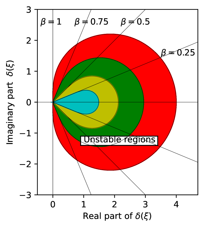
Figure 1: Unstable regions and $A$-stable tangent boundaries for the new FLMM

In Figure 1, the unstable regions and the A-stable tangent boundaries for fractional order values $\beta=0.25,0.5,0.75,1$ are shown.

6 Comparison of stability regions

We compare the stability regions of previously established implicit FLMMs of order 2 with our new FLMM which we now denote by NFLMM2 for want of an abbreviation.

For this, we consider the Lubich’s fractional backward difference method FBDF2 [13], the fractional Adams-Moulton method FAM1 [6] and the fractional Trapezoidal rule (FT2) [13], [9] given by their respective generating functions

$$\delta_{FBDF2}(\xi)=\left(\frac{3}{2}-2\xi+\frac{1}{2}\right)^{\beta},\quad\delta_{FAM1}(\xi)=\frac{(1-\xi)^{\beta}}{(1-\frac{\beta}{2})+\frac{\beta}{2}\xi}\quad\text{ and }\quad\delta_{FT2}(\xi)=\left(2\frac{1-\xi}{1+\xi}\right)^{\beta}.$$

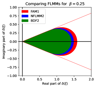
(a) $\beta=0.25$	(b) $\beta=0.50$
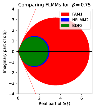
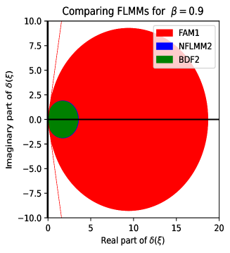
(c) $\beta=0.75$	(d) $\beta=0.90$

Figure 2: Comparing the unstable regions for NFLMM2 with other FLMMs for for $\beta=0.25,0.50,0.75,0.90$

In Figure 2, the unstable regions for these FLMMs and our NFLMM2 are shaded for various values of $\beta$. Note that the straight lines in the figures depicts the boundary of the stability region of the FT2 method in which the left side of the lines are the stability regions which are also correspond to the boundary of the analytical stability regions $\Sigma_{\beta}$. The unstable regions of FT2 arenot shaded for clarity.

The advantage of our NFLMM2 is, in terms of the unstable regions (UR), is that the UR of the NFLMM2 is smaller than that of FAM1 and is very much close to the UR of the FBDF2. Also, the UR of the FT2 is the largest among all the URs.

We note this from the observation that for the unstable regions ( see also the figures in Figure 2 )

$$\delta_{FBDF2}(-1)<\delta_{NFLMM2}(-1)<\delta_{FAM1}(-1)<\delta_{FT2}(-1)=+\infty.$$

Another interesting observation is that, as $\beta$ approaches 1, the UR of FAM1 rapidly expands to the unbounded UR of FT2 while the UR of our NFLMM2 gets closer to the bounded UR of FBDF2 with very slow expnasion.

This is confirmed from the fact, as $\beta$ approaches 1, that the generating function of the NFLMM2 converges to that of the FBDF2 while the generating function of the FAM1 converges to that of the FT2.

As for computational efficiency, the weights $w_{k}$ of NFLMM2 has the simplest computational effort as they involve only a linear combinations the Grünwald weights $g_{k}^{(\beta)}$ (see (32)).

Obviously, the weights of FBDF2 requires computations using the Miller’s formula (see eg. [6] ) with two previous weights.

The weights of FAM1 can be computed with the same amount of computation as that of NFLMM2. However, the right side of FAM1 scheme requires two coefficients from the Newton-Gregory expansion [6].

Finally, the weights of FT2 need more efforts as they require the first $n$ coefficients of its generating function and requires FFT to compute [9].

7 Conclusion

We proposed and analysed a new FLMM of order two for FIVPs that falls under a new type of FLMM that is different from previously known types. The new FLMM is $A$-stable as the other known order two methods. However, the proposed method outweighs the other methods in terms of stability and/or computational cost.

References

- [1] Aceto, L., Magherini, C., and Novati, P. On the construction and properties of m-step methods for fdes. SIAM Journal on Scientific Computing 37, 2 (2015), A653–A675.
- [2] Bonab, Z. F., and Javidi, M. Higher order methods for fractional differential equation based on fractional backward differentiation formula of order three. Mathematics and Computers in Simulation 172 (2020), 71–89.
- [3] Cameron, R., and McKee, S. Product integration methods for second-kind abel integral equations. Journal of computational and applied mathematics 11, 1 (1984), 1–10.
- [4] Diethelm, K. The analysis of fractional differential equations: An application-oriented exposition using differential operators of Caputo type. Springer Science & Business Media, 2010.
- [5] Galeone, L., and Garrappa, R. On multistep methods for differential equations of fractional order. Mediterranean Journal of Mathematics 3, 3 (2006), 565–580.
- [6] Galeone, L., and Garrappa, R. Fractional adams–moulton methods. Mathematics and Computers in Simulation 79, 4 (2008), 1358–1367.
- [7] Galeone, L., and Garrappa, R. Explicit methods for fractional differential equations and their stability properties. Journal of Computational and Applied Mathematics 228, 2 (2009), 548–560.
- [8] Garrappa, R. On some explicit adams multistep methods for fractional differential equations. Journal of computational and applied mathematics 229, 2 (2009), 392–399.
- [9] Garrappa, R. Trapezoidal methods for fractional differential equations: Theoretical and computational aspects. Mathematics and Computers in Simulation 110 (2015), 96–112.
- [10] Gunarathna, W. A., Nasir, H. M., and Daundasekera, W. B. An explicit form for higher order approximations of fractional derivatives. Applied Numerical Mathematics 143 (2019), 51–60.
- [11] Heris, M. S., and Javidi, M. On fractional backward differential formulas methods for fractional differential equations with delay. International Journal of Applied and Computational Mathematics 4, 2 (2018), 1–15.
- [12] Lubich, C. Fractional linear multistep methods for abel-volterra integral equations of the second kind. Mathematics of computation 45, 172 (1985), 463–469.
- [13] Lubich, C. Discretized fractional calculus. SIAM Journal on Mathematical Analysis 17, 3 (1986), 704–719.
- [14] Lubich, C. A stability analysis of convolution quadraturea for abel-volterra integral equations. IMA journal of numerical analysis 6, 1 (1986), 87–101.
- [15] Meerschaert, M. M., and Tadjeran, C. Finite difference approximations for fractional advection–dispersion flow equations. Journal of Computational and Applied Mathematics 172, 1 (2004), 65–77.
- [16] Nasir, H. M., Gunawardana, B. L. K., and Abeyrathna, H. M. N. P. A second order finite difference approximation for the fractional diffusion equation. International Journal of Applied Physics and Mathematics 3, 4 (2013), 237–243.
- [17] Nasir, H. M., and Kathija, A. A new type of fractional linear multi-step method with improved stability. Brazilian Symposium on Fractional calculus, Jan. 17, 2022.
- [18] Nasir, H. M., and Kathija, A. A new type of fractional linear multi-step method with improved stability. CQD – Revista Eletrônica Paulista de Matemática Accepted, 2022 (2022).
- [19] Nasir, H. M., and Nafa, K. Algebraic construction of a third order difference approximation for fractional derivatives and applications. ANZIAM Journal 59, EMAC2017 (2018), C231–C245.
- [20] Nasir, H. M., and Nafa, K. A new second order approximation for fractional derivatives with applications. SQU Journal of Science 23, 1 (2018), 43–55.
- [21] Oldham, K., and Spanier, J. The fractional calculus theory and applications of differentiation and integration to arbitrary order. Elsevier, 1974.
- [22] Podlubny, I. Fractional differential equations: an introduction to fractional derivatives, fractional differential equations, to methods of their solution and some of their applications, vol. 198. Academic press, 1998.
- [23] Young, A. The application of approximate product-integration to the numerical solution of integral equations. Proceedings of the Royal Society of London. Series A. Mathematical and Physical Sciences 224, 1159 (1954), 561–573.
- [24] Zhao, L., and Deng, W. A series of high-order quasi-compact schemes for space fractional diffusion equations based on the superconvergent approximations for fractional derivatives. Numerical Methods for Partial Differential Equations 31, 5 (2015), 1345–1381.