Target Sensing with Intelligent Reflecting Surface: Architecture and Performance

Abstract

Intelligent reflecting surface (IRS) has emerged as a promising technology to reconfigure the radio propagation environment by dynamically controlling wireless signal’s amplitude and/or phase via a large number of reflecting elements. In contrast to the vast literature on studying IRS’s performance gains in wireless communications, we study in this paper a new application of IRS for sensing/localizing targets in wireless networks. Specifically, we propose a new self-sensing IRS architecture where the IRS controller is capable of transmitting probing signals that are not only directly reflected by the target (referred to as the direct echo link), but also consecutively reflected by the IRS and then the target (referred to as the IRS-reflected echo link). Moreover, dedicated sensors are installed at the IRS for receiving both the direct and IRS-reflected echo signals from the target, such that the IRS can sense the direction of its nearby target by applying a customized multiple signal classification (MUSIC) algorithm. However, since the angle estimation mean square error (MSE) by the MUSIC algorithm is intractable, we propose to optimize the IRS passive reflection for maximizing the average echo signals’ total power at the IRS sensors and derive the resultant Cramer-Rao bound (CRB) of the angle estimation MSE. Last, numerical results are presented to show the effectiveness of the proposed new IRS sensing architecture and algorithm, as compared to other benchmark sensing systems/algorithms.

I Introduction

The future sixth-generation (6G) wireless systems need to enable the emerging location-aware applications such as virtual reality, robot navigation, autonomous driving, and so on. These applications impose more stringent requirements on both the communication and sensing performance of today’s wireless systems, such as ultra-high data rate, ubiquitous and seamless coverage, extremely-high reliability and ultra-low latency, as well as high-precision/resolution sensing [1, 2]. With the development of massive multi-input multi-output (MIMO) and millimeter wave (mmWave) communication technologies, the base station (BS) in communication systems has the capability to achieve high-resolution sensing in the angular domain. This thus gives rise to the emerging research area of joint communication and sensing, which advocates to share the hardware, platform, and radio resource in the design and use of communication and sensing systems to achieve their substantially enhanced performance with reduced cost [3, 4, 5, 6].

Specifically, in the conventional mono-static BS sensing system, the transmit and receive antennas are co-located at the BS or the BS antenna array is exploited for both transmitting and receiving radar probing signals in a full-duplex (FD) manner [7]. This mono-static sensing system generally entails a small number of angle-and-distance parameters to be estimated, due to the same direction-of-angle (DOA) and distance over the BS$\to$target and target$\to$BS links. However, the BS receive array may suffer non-negligible interference from its transmit array. Moreover, the localization performance of the BS is deteriorated with the increase of the target distance, due to the severe product-distance round-trip path-loss as well as random blockages between the BS and targets [8]. Alternatively, in the bi-static mobile sensing system, the transmit and receive arrays are placed in different sites (e.g., BSs and/or mobile devices). For example, a BS transmits probing signals, while a multi-antenna mobile device receives the echo signals reflected by the target for its localization. As such, the bi-static sensing system has the potential to improve the sensing performance over its mono-static sensing counterpart, due to the smaller product-distance path-loss and less susceptibility to interference, provided that the mobile device is near the target and far away from the BS. Nevertheless, the bi-static sensing system generally requires more parameters to be estimated for target localization, due to the different DOAs and distances over the BS$\to$target and target$\to$device links.

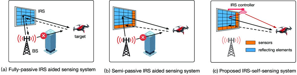
Figure 1: Different IRS-aided sensing systems.

To meet the high demands of future 6G systems in terms of both communication and sensing, the concept of smart radio environment has been recently proposed [9], which essentially leverages the digitally-controlled metasurface, termed intelligent reflecting surface (IRS) (or reconfigurable intelligent surface (RIS) equivalently), to reconfigure the wireless propagation environment in favor of both wireless communication and radar sensing [10, 11, 12, 13, 14]. In particular, by dynamically controlling phase shifts via a large number low-cost reflecting elements, IRS is able to realize many desired functions, such as bypassing environment obstacles, reshaping channel realizations/distributions, and increasing the multi-antenna/MIMO channel rank. These functions have been exploited and thoroughly investigated in the existing literature for improving the communication performance in various wireless systems, by developing efficient designs of IRS passive beamforming/reflection, channel estimation, and placement (see, e.g., [15, 16, 17, 18, 19, 20, 21]). On the other hand, in terms of radar sensing, IRS is able to establish a line-of-sight (LoS) link with the target in its vicinity, which is particularly helpful when the direct sensing link between the BS and target is blocked. Moreover, in addition to the direct BS-target link, IRS provides an extra LoS reflected link to sense the target from a different angle, thus potentially enhancing the sensing performance. The above benefits have motivated active research recently on designing different IRS systems/algorithms for improving the sensing performance.

Among others, a fully-passive IRS aided sensing system was studied in [22, 23, 24, 25, 26, 27], where an IRS without any transmit/receive radio-frequency (RF) chains is employed to help estimate the direction of a nearby target in the challenging scenario where the direct link between the BS and target is blocked. In this case, the BS sends probing signals, which are reflected by the IRS to illuminate the target with dynamically tuned beam directions. After the IRS-reflected beam hits the target, the echo signal is consecutively reflected by the target and IRS (again), and finally received at the BS, which estimates the direction of the target with respect to (w.r.t.) the IRS. However, this approach may suffer severe path-loss over the multiple (three-hop) signal reflections, i.e., BS$\to$IRS$\to$target$\to$IRS$\to$BS as shown in Fig. 1(a), and thus degraded DOA estimation performance. To tackle this issue, an alternative IRS-aided sensing method is to utilize the semi-passive IRS, where the IRS is equipped with dedicated (low-cost) sensors to receive signals for facilitating channel estimation in communications as well as target localization [28, 29, 30, 10]. Specifically, one efficient way is letting the IRS reflect the probing signals sent by the BS to the target, while the IRS sensors receive the echo signals reflected by the target for estimating its angle w.r.t. the IRS. Various approaches can be applied to estimate the target angle w.r.t. the IRS, such as Capon’s minimum variance method [31], maximum likelihood estimation (MLE) [32], and the subspace-based algorithms (e.g., multiple signal classification (MUSIC) algorithm [33] and estimation of signal parameters via rotational invariance techniques (ESPRIT) algorithm [34]). Nevertheless, the angle estimation performance is still constrained by the sensors’ received signal-to-noise ratio (SNR), due to the high path-loss of the two-hop signal reflections, i.e., BS$\to$IRS$\to$target$\to$sensors, as illustrated in Fig. 1(b).

To improve the sensing performance of the aforementioned IRS aided sensing systems, we propose in this paper a new IRS-self-sensing system as shown in Fig. 1(c), where the IRS reflecting elements are illuminated by the probing signals from the IRS controller in short distance and form reflected beams to sense the locations of its nearby targets. Moreover, receiving sensors are installed at the IRS to receive the echo signals from two types of links: 1) the two-hop IRS-reflected echo link, i.e., IRS controller$\to$IRS elements$\to$target$\to$IRS sensors; and 2) the one-hop direct echo link, i.e., IRS controller$\to$target$\to$IRS sensors. This thus greatly reduces the product-distance path-loss in the IRS-reflected echo link as compared to both the conventional fully- and semi-passive IRS aided sensing systems (see Figs. 1(a) and 1(b)), since the probing signals are transmitted from the IRS controller (instead of the BS) that is placed very close to the IRS reflecting elements in practice. Moreover, the MUSIC algorithm can be applied to estimate the target DOA with better resolution based on the received echo signals from both links at the IRS sensors. On the other hand, from a network implementation perspective, the self-sensing IRS does not involve the BS or any mobile device in the sensing process, hence greatly reducing the communication and control overhead required for target sensing. Thus, it is beneficial to deploy such low-cost self-sensing IRSs in the network to locate their nearby targets in a distributed manner, which can significantly alleviate the sensing task at the BS/device side in wireless networks. In the following, we summarize the main contributions of this paper.

First, we apply a customized MUSIC algorithm for our considered IRS-self-sensing system to estimate the DOA of a target near the IRS, based on the received echo signals over both the direct and IRS-reflected echo links. Although the DOA estimation MSE by the MUSIC algorithm is intractable, we formulate an optimization problem to optimize the IRS passive reflection for maximizing the average echo signals’ total power at IRS sensors. We show that in the presence of both the direct and IRS-reflected echo links, the discrete Fourier transform (DFT) based IRS passive reflection is optimal, which generates an omnidirectional beampattern in the angular domain for target sensing. Second, we show that the received signal power due to the IRS-reflected echo link linearly increases with the number of IRS reflecting elements, and it is larger than that due to the direct echo link when the number of IRS reflecting elements is sufficiently large. Moreover, we analytically show that it is beneficial to employ the IRS controller for sending probing signals as compared to the benchmark scheme by using instead a nearby mobile device. Furthermore, the Cramer-Rao bound (CRB) of the target DOA estimation MSE is analytically derived. Last, numerical results are presented to validate the performance gain of the proposed IRS-self-sensing system as compared to various benchmark sensing systems/algorithms.

The rest of this paper is organized as follows. We first present in Section II the proposed new IRS-self-sensing system and its sensing protocol. In Section III, we present the customized DOA estimation algorithm and the optimal IRS passive reflection for target sensing. Subsequently, we analytical show the advantages of the proposed new IRS architecture and the resultant CRB for the DOA estimation in Section IV. Numerical results are provided in Section V, followed by the conclusions in Section VI.

Notations: $\left\|\cdot\right\|_{2}$ denotes the Euclidean norm, $\text{vec}(\cdot)$ denotes the operation that stacks the columns of a matrix, $\mathrm{diag}({\bf x})$ denotes a diagonal matrix with the diagonal entries specified by vector ${\bf x}$. $\Re(x)$ and $\Im(x)$ denote the real and imaginary parts of a complex number $x$. For a complex symbol, $(\cdot)^{\dagger}$, $(\cdot)^{H}$, and $(\cdot)^{T}$ denote its complex conjugate, conjugate transpose, and transpose, respectively. For a square matrix $\mathbf{S}$, $\mathbf{S}\succeq 0$ means that $\mathbf{S}$ is positive semi-definite, and $\mathrm{tr}(\mathbf{S})$ denotes its trace. The Hadamard product is denoted by $\odot$, and the Kronecker product is denoted by $\otimes$. The distribution of a circularly symmetric complex Gaussian (CSCG) random variable with mean $u$ and covariance $\sigma^{2}$ is denoted by $\mathcal{CN}(u,\sigma^{2})$, $\backsim$ stands for “distributed as”, $\mathbb{E}(\cdot)$ denotes the statistical expectation, and $\dot{\mathbf{a}}(x)$ denotes the first-order partial derivative w.r.t. $x$.

II System Model

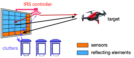
Figure 2: An IRS-self-sensing system.

We consider the proposed IRS-self-sensing system as shown in Fig. 2, where an IRS is deployed in the network to sense the location of an unknown target in the presence of $L$ clutters under the assumption that the IRS location is known a priori. The IRS consists of $N_{0}=N_{\rm h}\times N_{\rm v}$ reflecting elements, where $N_{\rm h}$ and $N_{\rm v}$ denote respectively the number of horizontal and vertical elements with the inter-element (horizontal and vertical) distance denoted by $d_{\rm I}$. The reflecting elements are illuminated by the probing signals from a single omnidirectional-antenna IRS controller that is capable of transmitting signals as well as dynamically controlling the IRS passive reflection for localizing the target. Moreover, to estimate both the azimuth and elevation angles of the target, $M_{0}$ (assumed to be an even number) sensors are installed adjacent to the IRS reflecting elements to receive the echoed signals by the target as shown in Fig. 2, where $M_{\rm h}=M_{\rm v}=(M_{0}+1)/2$ sensors are placed along the horizontal and vertical axes, respectively, with the inter-sensor distance given by $d_{\rm s}$. For simplicity, we focus on the target’s azimuth angle estimation in this paper based on the received signals on the $M_{\rm h}$ horizontal sensors, while the results can be extended to estimate its elevation angle as well.

II-A Radar Channel Model

We assume a narrow-band sensing system, where the IRS controller consecutively sends probing signals over $T$ snapshots, within which all the associated channels are assumed to remain static. At each snapshot, the sensors receive the signals transmitted from the IRS controller and that reflected by the target as well as clutters, with and without the IRS reflection. Specifically, the received signals reflected by the target undergo two types of links: 1) the two-hop IRS-reflected echo link, i.e., IRS controller$\to$IRS elements$\to$target$\to$IRS sensors; and 2) the single-hop direct echo link, i.e., IRS controller$\to$target$\to$IRS sensors. These two links are modeled as follows in detail, respectively.

First, consider the IRS-reflected echo link associated with the target. Let ${\bf u}(\bar{\vartheta},\bar{N})$ denote the steering vector function, which is defined as

$${\bf u}(\bar{\vartheta},\bar{N})\triangleq[e^{\frac{-\jmath(\bar{N}-1)\pi\bar{\vartheta}}{2}},e^{\frac{-\jmath(\bar{N}-3)\pi\bar{\vartheta}}{2}},\dots,e^{\frac{\jmath(\bar{N}-1)\pi\bar{\vartheta}}{2}}]^{T},$$ (1)

where $\bar{N}$ (assumed to be an even number) denotes the uniform linear array (ULA) size and $\bar{\vartheta}$ denotes the constant phase difference between the observations at two adjacent elements/sensors. Then, the IRS controller$\to$IRS elements channel, denoted by ${\bf h}_{{\rm CI}}\in\mathbb{C}^{N_{0}\times 1}$, can be modeled as follows based on the far-field LoS channel model.

$${\bf h}_{{\rm CI}}={\alpha}_{{\rm CI}}{\bf a}(\theta_{\rm CI,h},\theta_{\rm CI,v}),$$ (2)

where ${\alpha}_{{\rm CI}}=\sqrt{\frac{\lambda^{2}}{16\pi^{2}d_{\rm CI}^{2}}}e^{\frac{\jmath 2\pi d_{\rm CI}}{\lambda}}$ denotes the complex-valued path gain of the IRS controller$\to$IRS elements channel, $\lambda$ denotes the carrier wavelength, $d_{{\rm CI}}$ denotes the distance between the IRS controller and IRS central element, and $\theta_{\rm CI,h}\in[-\pi/2,\pi/2]$ and $\theta_{\rm CI,v}\in[-\pi/2,\pi/2]$ denote respectively the physical azimuth and vertical angles-of-arrival (AoA) at the IRS. Therein, ${\bf a}(\cdot)$ denotes the response vector function of the IRS, which is defined as

$${\bf a}(\theta_{\rm CI,h},\theta_{\rm CI,v})={\bf u}(\phi_{\rm CI,h},N_{\rm h})\otimes{\bf u}(\phi_{\rm CI,v},N_{\rm v}),$$ (3)

where $\phi_{\rm CI,h}\triangleq\frac{2d_{\rm I}}{\lambda}\sin(\theta_{\rm CI,h})\sin(\theta_{\rm CI,v})\in[-\frac{2d_{\rm I}}{\lambda},\frac{2d_{\rm I}}{\lambda}]$ and $\phi_{\rm CI,v}\triangleq\frac{2d_{\rm I}}{\lambda}\cos(\theta_{\rm CI,v})\in[-\frac{2d_{\rm I}}{\lambda},\frac{2d_{\rm I}}{\lambda}]$ are referred to as the horizontal and vertical spatial directions, respectively. Under the far-field condition, the AoAs from the target to IRS sensors can be assumed to be the same as the angles-of-departure (AoDs) from the IRS elements to target. As such, the echo channel of the IRS elements$\to$target$\to$IRS (horizontal) sensors link can be modeled as

$${\bf H}_{{\rm ITS}}=\alpha_{\rm r}{\bf b}(\theta_{\rm IT,h}){\bf a}^{T}(\theta_{\rm IT,h},\theta_{\rm IT,v}),$$ (4)

where $\theta_{\rm IT,h}$ and $\theta_{\rm IT,v}$ denote the azimuth and vertical AoDs from the IRS to target, respectively, ${\bf b}(\theta_{\rm IT,h})={\bf u}(\frac{2d_{\rm s}}{\lambda}\sin(\theta_{\rm IT,h}),M_{\rm h})\in\mathbb{C}^{M_{\rm h}\times 1}$ denotes the receive response vector from the target to IRS sensors, and $\alpha_{\rm r}=\beta_{\rm r}G_{\rm r}$ represents the complex-valued path gain with $\beta_{\rm r}\backsim\mathcal{CN}(0,1)$ denoting the small-scale complex channel gain and $G_{\rm r}=\sqrt{\frac{{{\lambda^{2}}\kappa}}{{64{\pi^{3}}{d_{\rm IT}^{4}}}}}$ denoting the signal attenuation caused by the propagation from IRS to the target and then from the target to IRS sensors as well as the scattering process. Therein, $d_{\rm IT}$ denotes the distance between the IRS and target, and $\kappa$ denotes the radar cross section (RCS), which is a measurement of power scattered in a given direction when a target is illuminated by an incident wave. Let ${\bm{\varphi}}_{0}[t]\in\mathbb{C}^{N_{0}\times 1}$ denote the IRS reflection vector at each snapshot $t\in\mathcal{T}\triangleq\{1,\cdots,T\}$ with each coefficient $[{\bm{\varphi}}_{0}[t]]_{n}=e^{\jmath\omega_{n}},n\in\{1,\cdots,N_{0}\}$ denoting the phase shift of IRS reflecting element $n$. Based on the above, the channel of the echo signal reflected from the target over the IRS-reflected link (i.e., IRS controller$\to$IRS elements$\to$target$\to$IRS sensors) at snapshot $t$ is given by

$${\bf g}_{\rm r}[t]={\bf H}_{{\rm ITS}}\mathrm{diag}({\bm{\varphi}}_{0}[t]){\bf h}_{{\rm CI}}$$

$$=\alpha_{\rm r}\alpha_{\rm CI}{\bf b}(\theta_{\rm IT,h}){\bf a}^{T}(\theta_{\rm IT,h},\theta_{\rm IT,v})\mathrm{diag}({\bm{\varphi}}_{0}[t]){\bf a}(\theta_{\rm CI,h},\theta_{\rm CI,v}).$$ (5)

Next, the direct echo link (i.e., IRS controller$\to$target$\to$IRS sensors) can be modeled as

$${\bf g}_{\rm d} =\alpha_{\rm d}{\bf b}(\theta_{\rm IT,h}),$$ (6)

where $\alpha_{\rm d}=\beta_{\rm d}G_{\rm d}$ denotes the complex-valued reflection path gain with $\beta_{\rm d}\backsim\mathcal{CN}(0,1)$ being the small-scale complex channel gain and $G_{\rm d}=\sqrt{\frac{{{\lambda^{2}}\kappa}}{{64{\pi^{3}}{d_{\rm CT}^{2}d_{\rm IT}^{2}}}}}$. Herein, $d_{\rm IT}$ denotes the distance between the IRS and target, and $d_{\rm CT}$ denotes the distance from the IRS controller to target. Note that ${\bf g}_{\rm d}$ remains static over $T$ snapshots.

On the other hand, for the clutters, let ${\bf g}_{{\rm r},I_{\ell}}[t]\in\mathbb{C}^{M_{\rm h}\times 1}$ and ${\bf g}_{{\rm d},I_{\ell}}\in\mathbb{C}^{M_{\rm h}\times 1}$ denote respectively the IRS-reflected and direct echo links associated with each clutter ${\ell}\in 1,\cdots,L$ at each snapshot $t$, which can be similarly modeled as (5) and (6) for the target. In addition, we denote by ${\bf h}_{{\rm CS}}\in\mathbb{C}^{M_{\rm h}\times 1}$ the IRS controller$\to$IRS sensors channel, which can be modeled similar to the IRS controller$\to$IRS elements channel in (2). As such, the received signals at the IRS (horizontal) sensors at each snapshot $t$ is given by

$${\bf y}_{0}[t] =\left({\bf g}_{\rm r}[t]+{\bf g}_{\rm d}+\underbrace{\sum_{\ell=1}^{L}({\bf g}_{{\rm r},I_{\ell}}[t]+{\bf g}_{{\rm d},I_{\ell}})+{\bf h}_{{\rm CS}}}_{\rm background~{}channel}\right)x[t]$$

$$+{\bf z}_{0}[t],t\in\mathcal{T},$$ (7)

where $x[t]$ is the signal sent by the IRS controller at snapshot $t$ which is simply set as $x[t]=1,\forall t$, and ${\bf z}_{0}[t]\in\mathbb{C}^{M_{\rm h}\times 1}\backsim\mathcal{CN}(\mathbf{0}_{M_{\rm h}},\sigma_{0}^{2}\mathbf{I}_{M_{\rm h}})$ denotes the zero-mean additive white Gaussian noise (AWGN) vector at snapshot $t$ with the normalized noise power $\sigma_{0}^{2}$.

II-B Proposed Protocol for IRS-enabled Target Angle Estimation

The signal model in (7) is assumed to be obtained in a particular range-Doppler bin of interest, for which the range and the Doppler parameters are omitted in the model. Thus, we focus on the (azimuth) angle estimation in this paper The main procedures consist of two phases, namely, the offline training phase that estimates the static background channel at the IRS sensors w.r.t. each IRS reflection pattern available, followed by the online estimation phase that tunes IRS reflections for estimating the target angle w.r.t. the IRS. Specifically, in the offline training, we assume that the environmental state remains unchanged over a much larger timescale than that of the real-time sensing and there is no target in the environment; while the IRS applies all reflection patterns/vectors in a predefined IRS reflection matrix (to be specified in Section III). As such, when the IRS applies the passive reflection vector ${\bm{\varphi}}$, the received signal vector at the IRS sensors is given by

$${{\bf y}}_{\rm int}({\bm{\varphi}})=\left(\underbrace{\sum_{\ell=1}^{L}({\bf g}_{{\rm r},I_{\ell}}({\bm{\varphi}})+{\bf g}_{{\rm d},I_{\ell}})+{\bf h}_{{\rm CS}}}_{{\bf g}_{\rm int}(\bm{\varphi}):~{}\rm background~{}channel}\right)x+\tilde{\bf z},$$ (8)

where ${\bf g}_{{\rm r},I_{\ell}}({\bm{\varphi}})$ depends on the IRS reflection vector $\bm{\varphi}$ in general. Thus, with $x=1$, the static background channel given IRS reflection vector $\bm{\varphi}$ can be estimated as $\hat{{\bf g}}_{\rm int}(\bm{\varphi})={{\bf y}}_{\rm int}({\bm{\varphi}})$, which includes the channels from the IRS controller and all nearby clutters to the IRS sensors. Next, consider the online estimation phase. For each IRS reflection vector ${\bm{\varphi}}_{0}[t]$ in snapshot $t$, undesired interference from the IRS controller and all clutters is first removed in the received signal ${\bf y}_{0}[t]$ based on the correspondingly estimated background channel, which yields

$${\bf y}[t] ={\bf y}_{0}[t]-\hat{{\bf g}}_{\rm int}(\bm{\varphi}[t])=({\bf g}_{\rm r}[t]+{\bf g}_{\rm d})x[t]+{\bf z}[t],$$

$$=\alpha_{\rm r}\alpha_{\rm CI}{\bf b}(\theta_{\rm IT,h}){\bf a}^{T}(\theta_{\rm IT,h},\theta_{\rm IT,v})\mathrm{diag}({\bm{\varphi}}_{0}[t]){\bf a}(\theta_{\rm CI,h},\theta_{\rm CI,v})$$

$$+\alpha_{\rm d}{\bf b}(\theta_{\rm IT,h})+{\bf z}[t],$$ (9)

where $\mathbf{z}[t]=(\mathbf{z}_{0}[t]-\tilde{\mathbf{z}})\sim\mathcal{CN}(\mathbf{0},\sigma^{2}\mathbf{I})$ with $\sigma^{2}\triangleq 2\sigma_{0}^{2}$. To facilitate the IRS passive reflection design over space and time, we denote ${\bm{\varphi}}_{0}[t]$ as the Hadamard product of two vectors, i.e., ${\bm{\varphi}}_{0}[t]={\bm{\varphi}}_{\rm h}[t]\otimes{\bm{\varphi}}_{\rm v}[t]$, where ${\bm{\varphi}}_{\rm h}=[e^{\jmath\omega_{1}},\cdots,e^{\jmath\omega_{N_{\rm h}}}]^{T}$ and ${\bm{\varphi}}_{\rm v}=[e^{\jmath\omega_{1}},\cdots,e^{\jmath\omega_{N_{\rm v}}}]^{T}$ are referred to as the horizontal and vertical IRS reflection vectors, respectively. Then, we have

$${s}({\bm{\varphi}}_{0}[t]) \triangleq{\bf a}^{T}(\theta_{\rm IT,h},\theta_{\rm IT,v})\mathrm{diag}({\bm{\varphi}}_{0}[t]){\bf a}(\theta_{\rm CI,h},\theta_{\rm CI,v})$$

$$=({\bf a}^{T}(\theta_{\rm IT,h},\theta_{\rm IT,v})\odot{\bf a}^{T}(\theta_{\rm CI,h},\theta_{\rm CI,v})){\bm{\varphi}}_{0}[t]$$

$$=({\bf u}^{T}(\phi_{\rm IT,h},N_{\rm h})\otimes{\bf u}^{T}(\phi_{\rm IT,v},N_{\rm v}))\odot({\bf u}^{T}(\phi_{\rm CI,h},N_{\rm h})$$

$$~{}~{}~{}\otimes{\bf u}^{T}(\phi_{\rm CI,v},N_{\rm v})){\bm{\varphi}}_{0}[t]$$

$$=[{\bf u}^{T}(\tilde{\phi}_{\rm IT,h},N_{\rm h})\otimes{\bf u}^{T}(\tilde{\phi}_{\rm IT,v},N_{\rm v})][{\bm{\varphi}}_{\rm h}[t]\otimes{\bm{\varphi}}_{\rm v}[t]]$$

$$=({\bf u}^{T}(\tilde{\phi}_{\rm IT,h},N_{\rm h}){\bm{\varphi}}_{\rm h}[t])\otimes({\bf u}^{T}(\tilde{\phi}_{\rm IT,v},N_{\rm v}){\bm{\varphi}}_{\rm v}[t]),$$ (10)

where $\tilde{\phi}_{\rm IT,h}\triangleq\phi_{\rm IT,h}+\phi_{\rm CI,h}$ and $\tilde{\phi}_{\rm IT,v}\triangleq\phi_{\rm IT,v}+\phi_{\rm CI,v}$. For simplicity, we assume that the IRS vertical reflection vector has been aligned. Thus, (II-B) can be simplified as

$${\bf y}[t] =\alpha_{\rm r}\alpha_{\rm CI}{\bf b}(\theta_{\rm IT,h}){\bf q}^{T}(\theta_{\rm IT,h}){\bm{\varphi}}_{\rm h}[t]\eta_{\rm r}+\alpha_{\rm d}{\bf b}(\theta_{\rm IT,h})+{\bf z}[t],$$ (11)

where ${\bf q}^{T}(\theta_{\rm IT,h})\triangleq{\bf u}^{T}(\tilde{\phi}_{\rm IT,h},N_{\rm h})\in\mathbb{C}^{1\times N_{h}}$ and $\eta_{\rm r}\triangleq{\bf u}^{T}(\tilde{\phi}_{\rm IT,v},N_{\rm v}){\bm{\varphi}}_{\rm v}[t]$. For ease of notation, in the sequel, we simply re-denote $\theta_{\rm IT,h}$ by $\theta$, $N_{\rm h}$ by $N$, $M_{\rm h}$ by $M$, $\bm{\varphi}_{\rm h}[t]$ by $\bm{\varphi}[t]$, and thus

$${\bf y}[t] =\gamma_{\rm r}{\bf b}(\theta){\bf q}^{T}(\theta){\bm{\varphi}}[t]+\alpha_{\rm d}{\bf b}(\theta)+{\bf z}[t]$$

$$={\bf b}(\theta){f}({\bm{\varphi}[t]})+{\bf z}[t],$$ (12)

with

$${f}({\bm{\varphi}[t]})=\gamma_{\rm r}{\bf q}^{T}(\theta){\bm{\varphi}}[t]+\alpha_{\rm d},$$ (13)

where $\gamma_{\rm r}=\alpha_{\rm r}\alpha_{\rm CI}\eta_{\rm r}$. Then, the DOA of the target (i.e., $\theta$) is estimated from $\{{\bf y}[t]\}_{t=1}^{T}$ by using the MUSIC algorithm, as elaborated in the next section. Note that different from the traditional MIMO radar/phased-array radar for target sensing [42], the IRS sensors in the proposed self-sensing IRS receive signals over the two links from the same echo angle, i.e., $\theta$, and hence achieving enhanced DOA estimation performance.

III IRS Passive Reflection Design and DOA Estimation

In this section, we design the IRS passive reflection for estimating the azimuth angle from the target based on the MUSIC algorithm.

III-A DOA Estimation

To estimate the DOA of the target by using the celebrated MUSIC algorithm, we first stack the received echo signals at the IRS sensors from the target, i.e., $\{{\bf y}[t]\}_{t=1}^{T}$, and express them in the following matrix form

$$\mathbf{Y} =[{\bf y}[1],\cdots,{\bf y}[T]]={\bf b}(\theta)[{f}({\bm{\varphi}}[1]),\cdots,{f}({\bm{\varphi}}[T])]+{\bf Z}$$

$$\triangleq{\bf b}(\theta){\bf f}^{H}+{\bf Z},$$ (14)

where $\mathbf{Z}\triangleq[\mathbf{z}[1],\cdots,\mathbf{z}[T]]\in\mathbb{C}^{M\times T}$ and ${\bf f}^{H}\triangleq[{f}({\bm{\varphi}}[1]),\cdots,{f}({\bm{\varphi}}[T])]\in\mathbb{C}^{1\times T}$. Thus, the covariance matrix of $\mathbf{Y}$ is given by

$$\mathbf{R}_{\mathbf{Y}}=\frac{1}{T}\mathbf{Y}\mathbf{Y}^{H}=\frac{1}{T}{\bf b}(\theta){\bf f}^{H}\,{\bf f}{\bf b}^{H}(\theta)+\sigma^{2}{\bf I}_{M},$$ (15)

Following the procedures of the MUSIC algorithm, the eigenvalue decomposition of $\mathbf{R}_{\mathbf{Y}}$ in (15) is first obtained as

$$\mathbf{R}_{\mathbf{Y}}=[\mathbf{U}_{s},\mathbf{U}_{z}]\begin{bmatrix}\bm{\Sigma}_{s}&&\\ &&\bm{\Sigma}_{z}\end{bmatrix}\begin{bmatrix}\mathbf{U}_{s}^{H}\\ \mathbf{U}_{z}^{H}\\ \end{bmatrix}$$ (16)

where $\mathbf{U}_{s}\in\mathbb{C}^{M\times 1}$ and $\mathbf{U}_{z}\in\mathbb{C}^{M\times(M-1)}$ are the eigenvectors that span the signal and noise subspaces, respectively. As $\mathbf{b}(\theta)$ is orthogonal to $\mathbf{U}_{z}$, the MUSIC spectrum parameter is given by

$$P_{\mathrm{MUSIC}}(\theta)=\frac{1}{\mathbf{b}(\theta)^{H}\mathbf{U}_{z}\mathbf{U}_{z}^{H}\mathbf{b}(\theta)}.$$ (17)

By finding the maximum value of (17) over $\theta$, the DOA of the target is estimated accordingly.

III-B IRS Reflection Design

Although it is difficult to characterize the DOA estimation MSE of the MUSIC algorithm, it has been shown in [43] that the MSE tends to decrease with the increase of the average received signal power at the sensors. This is intuitively expected, since with a larger signal power illuminating the target, the received SNR of the echo signals reflected by the target is also higher at the IRS sensors, thus leading to a lower DOA estimation MSE [44].

According to (II-B), the average received signal power at IRS sensors is given by

$$P(\{{\bm{\varphi}[t]}\})=\mathbb{E}\left[\frac{1}{T}\sum_{t=1}^{T}{f}^{\dagger}({\bm{\varphi}[t]}){\bf b}^{H}(\theta){\bf b}(\theta){f}({\bm{\varphi}[t]})\right]$$

$$=\mathbb{E}\left[\frac{M}{T}\sum_{t=1}^{T}{f}^{\dagger}({\bm{\varphi}[t]}){f}({\bm{\varphi}[t]})\right]$$

$$=\mathbb{E}\left[\frac{M}{T}\sum_{t=1}^{T}(\gamma_{\rm r}^{\dagger}{\bm{\varphi}}^{H}[t]{\bf q}^{\dagger}(\theta)+\alpha_{\rm d}^{\dagger})\left(\gamma_{\rm r}{\bf q}^{T}(\theta){\bm{\varphi}}[t]+\alpha_{\rm d}\right)\right]$$

$$=\mathbb{E}[\gamma_{\rm r}\gamma_{\rm r}^{\dagger}]\text{tr}(\mathbf{R_{\bm{\varphi}}B})+{M\mathbb{E}[\alpha_{\rm d}\alpha_{\rm d}^{\dagger}]}+\frac{M}{T}\mathbb{E}[\beta_{\rm r}\beta_{\rm d}^{\dagger}]G_{\rm r}G_{\rm d}\alpha_{\rm CI}\eta_{\rm r}$$

$$\times{\bf q}^{T}(\theta)\sum_{t=1}^{T}{\bm{\varphi}}[t]+\frac{M}{T}\mathbb{E}[\beta_{\rm r}^{\dagger}\beta_{\rm d}]G_{\rm r}G_{\rm d}\alpha_{\rm CI}^{\dagger}\eta_{\rm r}^{\dagger}\sum_{t=1}^{T}{\bm{\varphi}}^{H}[t]{\bf q}^{\dagger}(\theta),$$ (18)

where the expectation is taken w.r.t. the random small-scale fading coefficients $\beta_{\rm r}$ and $\beta_{\rm d}$, $\mathbf{R}_{\bm{\varphi}}=\frac{1}{T}\sum_{t=1}^{T}{\bm{\varphi}}[t]{\bm{\varphi}}^{H}[t]$, and $\mathbf{B}=M{\bf q}^{\dagger}(\theta){\bf q}^{T}(\theta)$. Since $\mathbb{E}[\beta_{\rm r}]=0$ and $\mathbb{E}[\beta_{\rm d}]=0$, we have

$$P(\{{\bm{\varphi}[t]}\})=\mathbb{E}[\gamma_{\rm r}\gamma_{\rm r}^{\dagger}]\text{tr}(\mathbf{R_{\bm{\varphi}}B})+{M\mathbb{E}[\alpha_{\rm d}\alpha_{\rm d}^{\dagger}]}.$$ (19)

We aim to optimize the IRS passive reflection vectors, $\{\bm{\varphi}[t]\}$, for maximizing $P(\{{\bm{\varphi}[t]}\})$, which is equivalent to maximizing $\mathrm{tr}(\mathbf{R_{\bm{\varphi}}B})$ for any given $\theta$. As the IRS has no prior knowledge of the target location, we aim to maximize $\text{tr}(\mathbf{R_{\bm{\varphi}}B})$ in the worst-case scenario w.r.t. $\mathbf{B}$, which is formulated as the following optimization problem

$$(\mathrm{P1}):~{} \!\!\!\!\mathop{\max}\limits_{\{\bm{\varphi}[t]\}}\mathop{\min}\limits_{\mathbf{B}}\text{tr}(\mathbf{R_{\bm{\varphi}}B})$$

$$\!\!\mathrm{s.t.}~{}[\mathbf{R}_{\bm{\varphi}}]_{n,n}=1,~{}~{}n\in\mathcal{N},$$ (20)

$$\!\!\!\!~{}~{}~{}~{}~{}~{}\mathbf{R}_{\bm{\varphi}}\succeq 0,~{}\mathbf{B}\succeq 0,$$ (21)

$$\!\!\!\!~{}~{}~{}~{}~{}~{}\lambda_{n}(\mathbf{B})\geq\epsilon,~{}~{}~{}n\in\mathcal{N},$$ (22)

$$\!\!\!\!~{}~{}~{}~{}~{}~{}|[\bm{\varphi}[t]]_{n}|=1,~{}~{}~{}n\in\mathcal{N},t\in\mathcal{T},$$ (23)

where $\mathcal{N}\triangleq\{1,\cdots,N\}$, $\epsilon\geq 0$ and the constraint in (22) is imposed to eliminate the trivial solution of $\mathbf{B}=0$. Similar to [44], it can be shown that the optimal solution to problem (P1) satisfies $\mathbf{R}^{*}_{\bm{\varphi}}=\mathbf{I}_{N}$. Let $\bm{\Theta}\triangleq[{\bm{\varphi}}[1],\cdots,{\bm{\varphi}}[T]]\in\mathbb{C}^{N\times T}$ and thus we have $\mathbf{R}_{\bm{\varphi}}=\frac{1}{T}\bm{\Theta}\bm{\Theta}^{H}=\mathbf{I}_{N}$. This indicates that the optimal passive reflection matrix $\bm{\Theta}^{*}$ should be an orthogonal matrix with each entry satisfying the unit-modulus constraint. For example, one such matrix for $\bm{\Theta}^{*}$ is the matrix that concatenates the first $N$ columns of a $T\times T$ DFT matrix with $T\geq N$, with each entry given by

$$[\bm{\Theta}]_{n,t}=e^{-j\frac{2\pi(t-1)(n-1)}{T}},~{}n\in\mathcal{N},t\in\mathcal{T}.$$ (24)

Note that in this case, the optimal passive reflection matrix generates an omnidirectional beampattern in the angular domain for scanning the target in all possible directions. This is expected since the omnidirectional IRS beampattern is optimal for the IRS-reflected echo link to locate the target direction, while the resultant random phase difference between the two signals (reflected by IRS and non-reflected by IRS) arriving at the target does not affect the average estimation performance.

IV Performance analysis

In this section, we first show the performance advantage of the proposed IRS sensing system as compared to a baseline IRS sensing system assisted by a mobile device/user. Then, we characterize the CRB of the DOA estimation MSE in the considered IRS sensing system.

IV-A Performance Gain

IV-A1 IRS-reflected versus direct echo links

First, we show that the IRS-reflected echo link dominates the direct echo link in the average received signal power at the IRS sensors, when the number of IRS reflecting elements is sufficiently large. To this end, we characterize the average powers of the signals over these two links as follows.

Lemma 1

With the IRS reflection matrix given in (24), the average received signal powers at the IRS sensors over the IRS-reflected and direct echo links, denoted by $P_{\rm r}$ and $P_{\rm d}$, respectively, are given by

$$P_{\rm r}=\frac{{{NM\eta_{\rm r}\lambda^{4}}\kappa}}{{1024{\pi^{5}}{d_{\rm IT}^{4}d_{{\rm CI}}^{2}}}},~{}~{}~{}~{}~{}P_{\rm d}=\frac{M{{\lambda^{2}}\kappa}}{{64{\pi^{3}}{d_{\rm CT}^{2}d_{\rm IT}^{2}}}}.$$ (25)

Proof: For the IRS-reflected echo link ${\bf g}_{\rm r}[t]$, the average received signal power is given by

$$P_{\rm r} =\frac{1}{T}\sum_{t=1}^{T}\mathbb{E}\left[(\gamma_{\rm r}^{\dagger}{\bm{\varphi}}^{H}[t]{\bf q}^{\dagger}(\theta){\bf b}^{H}(\theta))(\gamma_{\rm r}{\bf b}(\theta){\bf q}^{T}(\theta){\bm{\varphi}}[t])\right]$$

$$=\mathbb{E}[\gamma_{\rm r}\gamma_{\rm r}^{\dagger}]\text{tr}(\mathbf{R_{\bm{\varphi}}B})=NM\mathbb{E}[\gamma_{\rm r}\gamma_{\rm r}^{\dagger}]=\frac{{{NM\eta_{\rm r}\lambda^{4}}\kappa}}{{1024{\pi^{5}}{d_{\rm IT}^{4}}d_{{\rm CI}}^{2}}}.$$ (26)

Next, for the direct echo link ${\bf g}_{\rm d}[t]$, the average received signal power is given by

$$P_{\rm d} =\frac{1}{T}\sum_{t=1}^{T}\mathbb{E}\left[(\alpha_{\rm d}^{\dagger}{\bf b}^{H}(\theta))(\alpha_{\rm d}{\bf b}(\theta))\right]=\frac{{M{\lambda^{2}}\kappa}}{{64{\pi^{3}}{d_{\rm CT}^{2}d_{\rm IT}^{2}}}}.$$ (27)

$\Box$

Lemma 1 shows that the average power of the IRS-reflected echo link is linearly increasing with the number of IRS reflecting elements, i.e., $N$. Moreover, based on Lemma 1, we obtain the following result.

Lemma 2

The average power of the IRS-reflected echo link exceeds that of the direct echo link when

$$N\geq N_{\rm th}\triangleq\frac{d_{\rm IT}^{2}d_{\rm CI}^{2}16\pi^{2}}{\eta_{r}\lambda^{2}d_{\rm CT}^{2}}.$$

Lemma 2 shows that when the number of IRS reflecting elements is sufficiently large, the IRS-reflected echo link leads to a more dominant received signal power in the IRS-reflected echo link than the direct echo link. Moreover, to exploit this gain, it is desirable to place the IRS controller closer to IRS reflecting elements for reducing their path-loss in the IRS controller$\to$IRS elements link.

IV-A2 IRS controller versus mobile user for sending probing signals

Next, we show that the proposed IRS sensing architecture by exploiting the IRS controller to send probing signals achieves better estimation performance than a benchmark system that needs a nearby mobile user to send probing signals. Note that in this user-aided system, the estimation performance critically depends on the location of the assisting mobile user.

For ease of comparison, we consider a typical case where the mobile device locates at the $x$-axis with its position given by $(d_{\rm UI},0,0)$. As such, given the DOA of the target $\theta$ and the IRS elements-target distance $d_{\rm IT}$, the distance between the device and target is obtained as

$$d_{\mathrm{UT}}=\sqrt{d_{{\rm UI}}^{2}+d_{\mathrm{IT}}^{2}-2d_{{\rm UI}}d_{\mathrm{IT}}\cos(\theta)}.$$ (28)

For convenience, we set $\theta=0$ and consider the case where the device locates between the IRS and target, i.e., $0<d_{\rm UI}<d_{\rm IT}$. Note that in (28), the case with a sufficiently small $d_{\rm UI}$ reduces to the proposed IRS self-sensing system. Based on Lemma 1 and (28), we first derive the average power of the combined channel including both the IRS-reflected and direct echo links w.r.t. $d_{\rm UI}$ for the user-aided IRS sensing system as follows.

Lemma 3

For the user-aided IRS sensing system with $0<d_{\rm UI}<d_{\rm IT}$, the average power of the combined channel at the IRS sensors is given by

$$P_{\rm c}(d_{\rm UI}) =P_{\rm r}(d_{\rm UI})+P_{\rm d}(d_{\rm UI})$$

$$=MN\eta_{\rm r}\frac{{{\lambda^{4}}\kappa}}{{1024{\pi^{5}}{d_{\mathrm{IT}}^{4}}}d_{\rm UI}^{2}}$$

$$+\frac{M{{\lambda^{2}}\kappa}}{{64{\pi^{3}}{d_{\mathrm{IT}}^{2}(d_{\rm UI}^{2}+d_{\mathrm{IT}}^{2}-2d_{\rm UI}d_{\mathrm{IT}}\cos(\phi))}}}.$$ (29)

Then, the effects of $d_{\rm UI}$ on $P_{\rm r},P_{\rm d}$, and $P_{\rm c}$ are characterized as follows.

Lemma 4

For the user-aided IRS sensing system, as $d_{\rm UI}$ increases, we have

• $P_{\rm r}(d_{\rm UI})$ monotonically decreases;

• $P_{\rm d}(d_{\rm UI})$ monotonically increases;

• $P_{\rm c}(d_{\rm UI})$ first monotonically decreases and then increases.

Proof: The first two results on $P_{\rm r}(d_{\rm UI})$ and $P_{\rm d}(d_{\rm UI})$ can be easily obtained, since the device$\to$IRS link distance increases and the device$\to$target link distance decreases. For the combined link, it can be shown that the first-order derivative of $P_{\rm c}(d_{\rm UI})$ is

$$P_{\rm c}^{\prime}(d_{\rm UI})=\frac{-2NM\eta_{r}\lambda^{4}\kappa(d_{\rm IT}-d_{\rm UI})^{3}+32M\lambda^{2}\kappa\pi^{2}d_{\rm IT}^{2}d_{\rm UI}^{3}}{1024\pi^{5}d_{\rm IT}^{4}d_{\rm UI}^{3}(d_{\rm IT}-d_{\rm UI})^{3}}.$$ (30)

Then, it follows that there exists a ${\bar{d}}_{\rm UI}$, such that $P_{\rm c}^{\prime}(d_{\rm UI})<0$ when $0<d_{\rm UI}<{\bar{d}}_{\rm UI}$ and $P_{\rm c}^{\prime}(d_{\rm UI})\geq 0$ when ${\bar{d}}_{\rm UI}\leq d_{\rm UI}<d_{\rm UT}$, thus leading to the desired result.  $\Box$

Lemma 4 shows that when the mobile device locates closer to the IRS as compared to the target, the IRS-reflected echo link yields a much larger power than the direct echo link in the average due to the prominent IRS passive beamforming gain. In contrast, when the mobile user gets closer to the target, the channel gain of the direct echo link is greatly enhanced due to the smaller path-loss from the user to the target, while the IRS-reflected echo link is severely attenuated.

Example 1

In Figs. 3 and  4, we plot the DOA estimation MSE by the MUSIC algorithm and average received signal power at the IRS sensors, respectively. We set $d_{\mathrm{IT}}=30$ m, $N=64$. It is observed that for the case with $d_{\rm UI}=0.47$ m, the direct echo link and IRS-reflected echo link achieve the same signal power at the sensors and thus the same MSE performance, which is consistent with Lemmas 1 and 2. In addition, it is observed that as $d_{\rm UI}$ increases, $P_{\rm c}$ first decreases and then increases. In contrast, the DOA estimation MSE first increases and then decreases with $d_{\rm UI}$. By letting $P_{\rm c}^{\prime}(d_{\rm UI})=0$ (see (30)), we obtain that $P_{\rm c}(d_{\rm UI})$ achieves its minimum value when $d_{\rm UI}=1.7852$ m, which also achieves the maximum MSE.

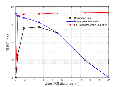
Figure 3: Effect of $d_{\rm UI}$ on the DOA estimation MSE.

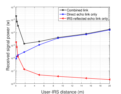
Figure 4: Effect of $d_{\rm UI}$ on the received signal power.

Remark 1

Example 1 shows that it is beneficial to employ the helping mobile device near either the IRS or the target for target localization, such that the DOA estimation MSE is minimized. Note that the former case exploits the IRS passive beamforming gain, while the latter case mainly relies on the short-distance user-target link for DOA estimation. However, in practice, since the availability of such helping user is random and so is its location, the estimation performance of the user-aided IRS sensing system is not guaranteed. In contrast, using the IRS controller as the probing signal transmitter (which is equivalent to the case of short user-IRS distance in Example 1) avoids this issue and thus offers a more predictable estimation performance than the user-aided IRS sensing system.

IV-B Cramer-Rao Bound

Since the DOA estimation MSE of the MUSIC algorithm is difficult to obtain, we analyze in this subsection the CRB of the proposed IRS self-sensing system that characterizes a lower bound of the DOA estimation MSE. Moreover, we gain useful insights into the effects of the number of IRS reflecting elements or sensors on the estimation performance.

First, we obtain the following result of the CRB for the target DOA estimation accuracy in the proposed IRS self-sensing system.

Theorem 1

For the proposed IRS self-sensing system, the CRB of the target DOA estimation MSE is given by (31) at the top of next page,

$$\mathrm{CRB}(\theta)\!=\!\frac{1/2}{\frac{T|\xi\alpha_{\rm{CI}}\eta_{\rm r}|^{2}}{\sigma^{2}}\!\left(\!w_{2}\frac{N^{3}-N}{6}\varsigma^{2}(\theta)M+\!w_{1}\frac{M^{3}-M}{6}\cos^{2}(\theta)N\!+\!w_{1}\frac{(M^{3}-M)}{6}\frac{\cos^{2}(\theta)}{\alpha_{\rm CI}\alpha_{\rm CI}^{\dagger}\eta_{\rm r}\eta_{\rm r}^{\dagger}}\!+\!w_{1}\frac{(M^{3}-M)}{6}\cos^{2}(\theta)p(\theta)\right)\!}.\!\!$$ (31)

where

$$w_{1}\! =\!\frac{\pi^{2}d_{\rm s}^{2}}{\lambda^{2}},~{}~{}w_{2}\!=\!\frac{\pi^{2}d_{\rm I}^{2}}{\lambda^{2}},~{}~{}\xi\!=\!\max(\alpha_{\rm r},\alpha_{\rm d}),$$

$${\varsigma}(\theta)\! =\!\cos(\theta)\sin(\theta_{\rm IT,v})\!+\sin(\theta_{\rm CI,h})\sin(\theta_{\rm CI,v}),$$

$$p(\theta)\! =\!\Re\left\{\frac{2}{T\alpha_{\rm CI}^{\dagger}\eta_{\rm r}^{\dagger}}\sum_{t=1}^{T}\!\left({{\bm{\varphi}}[t]_{1}e^{j(N-1)\pi\frac{{\rm d_{I}}}{\lambda}\bar{\varsigma}(\theta)}}+\cdots\right.\right.$$

$$\left.\left.+{{\bm{\varphi}}[t]_{N}e^{-j(N-1)\pi\frac{{\rm d_{I}}}{\lambda}\bar{\varsigma}(\theta)}}\!\right)\!\right\},$$

$$\bar{\varsigma}(\theta) =\sin(\theta)\sin(\theta_{\rm IT,v})\!+\sin(\theta_{\rm CI,h})\sin(\theta_{\rm CI,v}),$$

with ${\bm{\varphi}}[t]_{n}$ being the $n$th element of vector ${\bm{\varphi}}[t]$.

Proof: Please refer to Appendix A.  $\Box$

Remark 2

Theorem 1 shows that the CRB of the DOA estimation MSE decreases with both the number of IRS sensors, $M$, and that of IRS reflecting elements, $N$. Specifically, in the denominator of (31), the first two terms show the effects of the IRS-reflected echo link on the CRB performance, while the third term (i.e., $\frac{T|\xi|^{2}}{\sigma^{2}}(\!w_{1}\frac{M^{3}-M}{6}\cos^{2}(\theta))$) shows the effect of the direct echo link. The last term shows the effect of the IRS-reflected echo link and the direct echo link. Such results reveal that when $|\alpha_{\rm{CI}}\eta_{\rm r}|^{2}$ is small, a large number of IRS reflecting elements (i.e., a large $N$) is needed to compensate the severe path-loss due to the two-hop signal reflections in the IRS-reflected echo link. On the other hand, increasing the number of IRS sensors can improve the performance as it is beneficial for boosting the estimation SNR of the received signals over both the direct and IRS-reflected echo links.

V Numerical Results

TABLE I: Simulation parameters

Parameter	Value
Number of IRS reflecting elements	$N=64$
Number of IRS sensors	$M=8$
Distance from IRS to target	$d_{\rm IT}=30$ m
Angle of target w.r.t. IRS	$\theta=60^{\circ}$
Target RCS	$\kappa=7$ dBsm
Noise power	$-109$ dBm
Wavelength	$\lambda=0.2$ m
Number of BS transmit antennas	$64$
Number of BS receive antennas	$8$
Distance from IRS to BS	$d_{\rm BI}=100$ m
Angle of BS w.r.t. IRS	$\theta_{\rm I}=80^{\circ}$
Angle of IRS w.r.t. BS	$\theta_{\rm B}=80^{\circ}$
Distance from IRS controller to reflecting elements	$d_{\rm CI}=0.5$ m
Successful angle estimation threshold	$\delta=0.01$
Number of snapshots	$T=64$
Angle of device w.r.t. IRS	$60^{\circ}$
Distance from helping user to IRS	Uniformly distributed in $[0.5,100]$ m or $[0.5,135]$ m

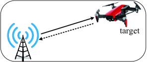
(a) BTB scheme

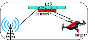
(b) BITS scheme

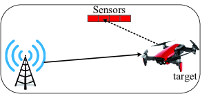
(c) BTS scheme

(d) BITIB scheme

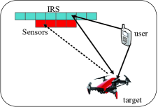
(e) Mobile-user aided scheme (MUS)

Figure 5: Different benchmark sensing systems with/without IRS.

In this section, we present numerical results to evaluate the performance of the proposed IRS-self-sensing system. For simplicity, we consider a ULA IRS as shown in Fig. 6, where the IRS is equipped with $N=64$ reflecting elements and $M=8$ sensors. The distance between the IRS and target is $d_{\rm IT}=30$ m, the azimuth angle of the target w.r.t. the IRS is set as $\theta=60^{\circ}$. Moreover, for the benchmark schemes detailed in the sequel, we consider there is a BS equipped with $64$ transmit antennas and $8$ receive antennas, where the distance between the IRS and BS is set as $d_{\rm BI}=100$ m. The other simulation parameters are set according to Table I, unless stated otherwise. It is worth noting that the IRS controller in our considered system is practically located in the far-field of ‘each IRS element’ due to its small size as composed to the distance with the controller. The DOA estimation performance is evaluated in terms of root mean square error (RMSE) and probability of successful estimation. Specifically, RMSE is defined as $\textrm{RMSE}\triangleq\sqrt{\mathbb{E}[(\theta-\hat{\theta})^{2}]}$, where $\hat{\theta}$ is the estimation of $\theta$. A target is said to be localized successfully in a given trial if $|\hat{\theta}-\theta|\leq\delta$ with a tunable constant $\delta$ [45, 46]. Herein, $\delta$ is set to be $0.01$.

We consider the following benchmark schemes that include the traditional radar system and the schemes that apply IRS in different ways to form the echo links to estimate the DOA of the target.

• BTB scheme: As illustrated in Fig. 5(a), the BS transmits and receives probing signals for target sensing; thus the echo link is BS$\to$target$\to$BS.

• BITS scheme: As illustrated in Fig. 5(b), the BS transmits probing signals, which are reflected by the IRS and received by its sensors; thus the echo link is BS$\to$IRS elements$\to$target$\to$ IRS sensors.

• BTS scheme: As illustrated in Fig. 5(c), the BS transmits probing signals, which are reflected by the target and received by its sensors; thus the echo link is BS$\to$target$\to$ IRS sensors.

• BITIB scheme: As illustrated in Fig. 5(d), the BS transmits probing signals, which are consecutively reflected over the BS$\to$IRS elements$\to$target$\to$IRS elements$\to$BS echo link.

• Mobile-user aided scheme (MUS): This scheme, as illustrated in Fig. 5(e) and previously considered in Example 1, is similar to our proposed scheme, while except that the probing signals are sent by a mobile user (instead of the IRS controller) whose location is random in practice.

Note that for the BITIB scheme, the DOA of target is estimated by the on-grid beam training method due to the lack of IRS sensors; while the MUSIC algorithm is applied to estimate the target DOA in the other benchmark schemes.

In Fig. 7, we show the RMSE of the proposed IRS self-sensing scheme versus BS transmit power. It is observed that the proposed scheme exhibits superior performance than the other benchmark schemes in the entire transmit power range. This is because, in the proposed IRS self-sensing scheme, the IRS is placed near the target with its controller and sensors for transmitting and receiving signals, respectively. As such, the signal traveling distance from the transmitter to the target and then to the receiver is much shorter than that of the BTB, BITS, BTS, and BITIB schemes. Note that in these four benchmark schemes, the signal is sent by the far-away BS, thus suffering severe path-loss. Moreover, the proposed IRS scheme can receive signals over both the direct and IRS-reflected echo links at the same time. As stated in Lemma 3, the proposed scheme with the combined links performs better than those based on the individual link only. Thus, the proposed IRS-self-sensing scheme that exploits both the IRS passive beamforming gain and the direct echo link gain for target DOA estimation is practically appealing. Besides, the proposed scheme substantially improves the RMSE performance as compared to the MUS scheme, since the latter scheme cannot guarantee that there always exists a helping device near the IRS/target.

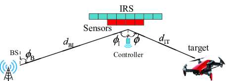
Figure 6: Simulation setup.

In Fig. 8, we evaluate the probability of successful estimation of the proposed scheme versus the transmit power against the other benchmark schemes. It is observed that the proposed scheme attains a much higher successful estimation probability than the other schemes. Moreover, the successful estimation probability of all schemes increases with the transmit power due to the increased received SNR at the BS/sensors. It is observed that when the distance from helping user to IRS is short, e.g., [0.5, 100] m, the proposed scheme performs worse than the MUS scheme in terms of probability of successful estimation in the low transmit power region, while it attains better performance when the transmit power increases. The reason is that when the transmit power is small, our proposed IRS self-sensing system has a low probability of successful estimation due to the low receive SNR at the sensors; while the MUS scheme has the potential to attain a higher probability of successful estimation, since the user has some likelihood to be located in the vicinity of the target which leads to higher DOA estimation accuracy. On the other hand, in the high-transmit power region, the proposed IRS self-sensing system achieves a high probability of successful estimation at high SNR, while the MUS scheme suffers some performance loss, since the user may be far away from the target and/or IRS and thus become the performance bottleneck.

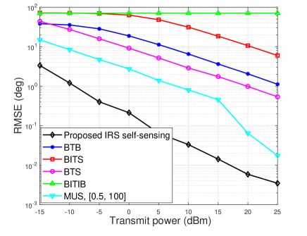
Figure 7: RMSE versus transmit power.

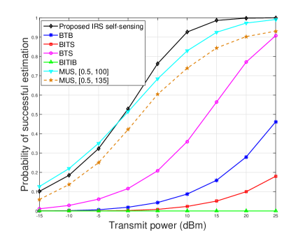
Figure 8: Probability of successful estimation versus transmit power.

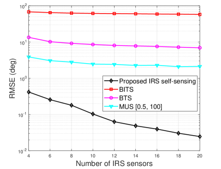
Figure 9: RMSE versus number of IRS sensors.

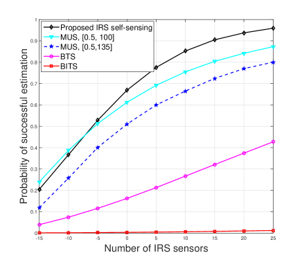
Figure 10: Probability of successful estimation versus number of IRS sensors.

Next, we investigate the impact of the number of sensors on the performance of the proposed IRS-self-sensing scheme in Fig. 9 and Fig. 10. It is observed that the estimation performance is critically dependent on the number of IRS sensors, i.e., $M$. Specifically, an increasing $M$ leads to a decreasing NMSE and an increasing probability of successful estimation for all schemes. One can observe that the proposed IRS-self-sensing scheme requires a small number of sensors for achieving a high DOA estimation accuracy as compared to the BITS, BTS, and MUS schemes that all use IRS sensors to receive signals. Note that there also exists a threshold on the number of sensors, above which the proposed IRS self-sensing system achieves a higher probability of successful estimation. This is fundamentally due to the increasing average SNR at the sensors with the increasing number of IRS sensors; thus similar arguments as for the effect of transmit power (see Fig. 8) apply. Moreover, the performance gap of the proposed scheme against other benchmark schemes is enlarged as the number of sensors increases.

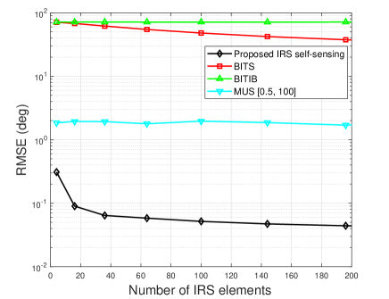
Figure 11: RMSE versus number of IRS reflecting elements.

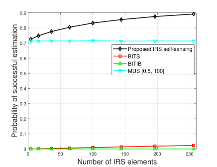
Figure 12: Probability of successful estimation versus number of IRS reflecting elements

.

In Fig. 11 and Fig. 12, we show the impact of the number of IRS reflecting elements on the sensing performance. It is observed that the proposed scheme obviously outperforms the schemes that sends the signal from BS or user. For the proposed scheme, the NMSE monotonically decreases with the IRS reflecting elements, i.e., $N$ and the probability of successful estimation monotonically increases with $N$. The reason is that as the number of IRS reflecting elements increases, the IRS passive beamforming gain continues to increase. However, the sensing performance of benchmark schemes does not improve too much when $N$ increases, since for those schemes, the IRS passive beamforming gain cannot greatly compensate the path-loss, especially in the case of far-away BS$\to$ IRS link. It is observed that as $N$ increases, the RMSE (or the probability of successful estimation) of the proposed scheme first rapidly decreases (increases) and then more slowly when $N$ is sufficiently large.

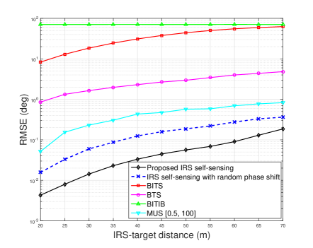
Figure 13: RMSE versus distance between IRS/sensors and target.

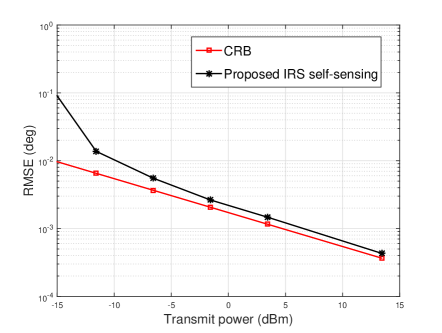
Figure 14: CRB and IRS self-sensing performance for DOA estimation.

In Fig. 13, we show the NMSE performance of different sensing schemes versus the IRS/sensors-target distance. It is observed that the proposed scheme achieves a small NMSE even at a long sensing range, thanks to the IRS controller in short distance with the reflecting elements. In contrast, the other benchmark schemes suffer a poor NMSE performance when the target is far from the IRS/sensors. Since the signal traveling distance from the transmitter to the receiver is too long, the average received signal power at IRS sensors is extremely low and the target cannot be sensed at long distances. Moreover, compared with the random-phase scheme that randomly generates IRS reflection over time, our proposed IRS reflection design for target sensing achieves a much smaller RMSE, since it yields an omnidirectional beampattern for target sensing.

Last, we compare in Fig. 14 the RMSE of the proposed IRS-self-sensing scheme by using the MUSIC algorithm and its CRB in Theorem 1. It is observed that although there is a notable gap in the low transmit power regime, the achieved NMSE of the proposed scheme gets very close to the obtained CRB when the transmit power is sufficiently large. This demonstrates the effectiveness of the proposed IRS-self-sensing scheme.

VI Conclusion

In this paper, we proposed a new IRS-self-sensing system, where the IRS controller is employed to transmit probing signals, and dedicated sensors are installed at the IRS for location/angle estimation based on the reflected signals by the target with and without the IRS reflection. The MUSIC algorithm was applied to estimate the DOA of the target in the IRS’s vicinity with high accuracy, without the involvement of either the BS or any mobile device. Although the DOA estimation MSE by the MUSIC algorithm is intractable, we optimized the IRS passive reflection matrix for maximizing the average received signals’ total power at the IRS sensors, which leads to the minimum MSE. Besides, we analytically showed that it is beneficial to employ the IRS controller (instead of a helping mobile device at random location) for sending probing signals, and obtained the CRB for the target DOA estimation.

Appendix A Proof of Theorem 1

We first introduce an auxiliary variable $\mathbf{c}=[0,\cdots,\frac{1}{\alpha_{\rm{CI}}\eta_{r}},\cdots,0]^{T}\in\mathbb{R}^{N\times 1}$. Then, (II-B) can be rewritten as

$${\bf y}[t] =\alpha_{\rm r}\alpha_{\rm{CI}}\eta_{\rm r}{\bf b}(\theta){\bf q}^{T}(\theta){\bm{\varphi}}[t]+\alpha_{\rm d}{\bf b}(\theta)+{\bf z}[t]$$

$$\overset{(a_{1})}{=}\alpha_{\rm{CI}}\eta_{\rm r}{\bf b}(\theta){\bf q}^{T}(\theta)\left(\alpha_{\rm r}{\bm{\varphi}}[t]+\alpha_{\rm d}\mathbf{c}\right)+{\bf z}[t],$$ (32)

where we use the property $\alpha_{\rm{CI}}\eta_{\rm r}{\bf q}^{T}(\theta){\bf c}=1$ in $(a_{1})$. Without loss of generality, by setting $\xi=\max(\alpha_{\rm r},\alpha_{\rm d})$, (A) can be approximated as

$${\bf y}[t]\approx\xi\alpha_{\rm{CI}}\eta_{\rm r}{\bf b}(\theta){\bf q}^{T}(\theta)\left({\bm{\varphi}}[t]+\mathbf{c}\right)+{\bf z}[t].$$ (33)

Since ${\bf z}[t]$ is CSCG distributed, the received signal at the sensors, ${\bf y}[t]$, can be modeled as an independent CSCG vector, i.e., ${\bf y}[t]\sim\mathcal{CN}(\xi\alpha_{\rm{CI}}\eta_{\rm r}{\bf b}(\theta){\bf q}^{T}(\theta)\left({\bm{\varphi}}[t]+\mathbf{c}\right),\sigma^{2}\mathbf{I})$.

$$\mathrm{CRB}(\theta)=\frac{1}{2\frac{T|\xi\alpha_{\rm{CI}}\eta_{\rm r}|^{2}}{\sigma^{2}}\left({\bf q}^{H}(\theta)\mathbf{R}^{T}_{\rm c}{\bf q}(\theta)\left\|\dot{\bf b}(\theta)\right\|_{2}^{2}+M\dot{\bf q}^{H}(\theta)\mathbf{R}^{T}_{\rm c}\dot{\bf q}(\theta)-\frac{M|{\mathbf{q}}^{H}(\theta)\mathbf{R}^{T}_{\rm c}\dot{\mathbf{q}}(\theta)|^{2}}{{\bf q}^{H}(\theta)\mathbf{R}^{T}_{\rm c}{\bf q}(\theta)}\right)}.$$ (49)

$${\bf q}^{H}(\theta)\mathbf{R}^{T}_{\rm c}{\bf q}(\theta)\left\|\dot{\bf b}(\theta)\right\|_{2}^{2}=4\sum_{m=1,2,\cdots,\frac{M-1}{2}}\pi^{2}\frac{d_{\rm s}^{2}}{\lambda^{2}}m^{2}\cos^{2}(\theta)\left(N+\frac{1}{\alpha_{\rm CI}\alpha_{\rm CI}^{\dagger}\eta_{\rm r}\eta_{\rm r}^{\dagger}}\right.$$

$$\left.+\underbrace{\Re\left\{\frac{2}{T\alpha_{\rm CI}^{\dagger}\eta_{\rm r}^{\dagger}}\sum_{t=1}^{T}\left({{\bm{\varphi}}[t]_{1}e^{j(N-1)\pi\frac{{\rm d_{I}}}{\lambda}\bar{\varsigma}(\theta)}}+\cdots+{{\bm{\varphi}}[t]_{N}e^{-j(N-1)\pi\frac{{\rm d_{I}}}{\lambda}\bar{\varsigma}(\theta)}}\right)\right\}}_{p(\theta)}\right)$$

$$=\frac{M^{3}-M}{6}\pi^{2}\frac{d_{\rm s}^{2}}{\lambda^{2}}\cos^{2}(\theta)\left(N+\frac{1}{\alpha_{\rm CI}\alpha_{\rm CI}^{\dagger}\eta_{\rm r}\eta_{\rm r}^{\dagger}}+p(\theta)\right),$$ (53)

Let $\bm{\varpi}=[\theta,\bar{\bm{\xi}}]^{T}$ denote the vector of unknown parameters to be estimated, which includes the DOA and the complex amplitudes with $\bar{\bm{\xi}}=[\Re\{\xi\},\Im\{\xi\}]^{T}$. The log-likelihood function for estimating $\bm{\varpi}$ from $\mathbf{Y}=({\bf y}[1],\cdots,{\bf y}[T])$ can be derived as

$$\log f_{\mathbf{Y}}(\mathbf{Y};\bm{\varpi})=\bar{f}_{1}(\mathbf{Y})+\bar{f}_{2}(\bm{\varpi})+\bar{f}_{3}(\mathbf{Y},\bm{\varpi}),$$ (34)

where $\bar{f}_{1}(\mathbf{Y})=-MN\log(\pi\sigma^{2})-\frac{1}{\sigma^{2}}\sum_{t=1}^{T}\left\|{\bf y}[t]\right\|_{2}^{2}$, and $\bar{f}_{2}(\bm{\varpi})$ is given by

$$\bar{f}_{2}(\bm{\varpi})=-\frac{1}{\sigma^{2}}\sum_{t=1}^{T}\left\|\xi\alpha_{\rm{CI}}\eta_{\rm r}{\bf b}(\theta){\bf q}^{T}(\theta)\left({\bm{\varphi}}[t]+\mathbf{c}\right)\right\|_{2}^{2}$$

$$\!=\!-\frac{1}{\sigma^{2}}\sum_{t=1}^{T}\xi^{\dagger}\xi\alpha_{\rm{CI}}^{\dagger}\alpha_{\rm{CI}}\eta_{\rm r}^{\dagger}\eta_{\rm r}\!\left(\!{\bm{\varphi}}^{H}[t]\!+\!\mathbf{c}^{H}\!\right)\!\mathbf{A}^{H}(\theta)\mathbf{A}(\theta)\left({\bm{\varphi}}[t]\!+\!\mathbf{c}\right)$$

$$=-\frac{T}{\sigma^{2}}\xi^{\dagger}\xi\alpha_{\rm{CI}}^{\dagger}\alpha_{\rm{CI}}\eta_{\rm r}^{\dagger}\eta_{\rm r}\text{tr}(\mathbf{A}(\theta)\mathbf{R}_{c}\mathbf{A}^{H}(\theta)),$$ (35)

where $\mathbf{A}(\theta)={\bf b}(\theta){\bf q}^{T}(\theta)$ and

$$\mathbf{R}_{c}=\frac{1}{T}\sum_{t=1}^{T}\left({\bm{\varphi}}[t]+\mathbf{c}\right)\left({\bm{\varphi}}^{H}[t]+\mathbf{c}^{H}\right).$$ (36)

Moreover, $\bar{f}_{3}(\mathbf{Y},\bm{\varpi})$ is given by

$$\bar{f}_{3}(\mathbf{Y},\bm{\varpi})\!=\!\frac{2}{\sigma^{2}}\Re\!\left\{\!\xi^{\dagger}\alpha_{\rm{CI}}^{\dagger}\eta_{\rm r}^{\dagger}\sum_{t=1}^{T}\!\left(\!{\bm{\varphi}}^{H}[t]+\mathbf{c}^{H}\!\right)\!{\bf q}^{\dagger}(\theta){\bf b}(\theta)^{H}{\bf y}[t]\!\right\}$$

$$\!=\!\frac{2\sqrt{T}}{\sigma^{2}}\Re\!\left\{\!\xi^{\dagger}\alpha_{\rm{CI}}^{\dagger}\eta_{\rm r}^{\dagger}\sum_{n=1}^{N}\mathbf{A}_{:,n}^{H}(\theta)\left(\frac{1}{\sqrt{T}}\sum_{t=1}^{T}{\bf y}[t]\!\left(\!{\bm{\varphi}}^{\dagger}_{n}[t]\!+\!\mathbf{c}^{\dagger}_{n}\!\right)\!\right)\!\right\},$$ (37)

where $\mathbf{c}^{\dagger}_{n}$ denotes the $n$-th element of vector $\mathbf{c}^{\dagger}$. It is observed from (A) that

$$\bar{\bf v}_{n}=\frac{1}{\sqrt{T}}\sum_{t=1}^{T}{\bf y}[t]\left({\bm{\varphi}}^{\dagger}_{n}[t]+\mathbf{c}^{\dagger}_{n}\right),\forall n\in\mathcal{N},$$ (38)

is the sufficient statistic [47], which contains all information relevant to $\bm{\varpi}$ derived from data $\mathbf{Y}$. In order to reduce the dimensionality and computational complexity, instead of using log-likelihood function in (34), we derive the fisher information matrix (FIM) [40] in the following sufficient statistic matrix:

$${{\bf V}}=[\bar{\bf v}_{1},\cdots,\bar{\bf v}_{N}]=\frac{1}{\sqrt{T}}\sum_{t=1}^{T}{\bf y}[t]\left({\bm{\varphi}}^{H}[t]+\mathbf{c}^{H}\right).$$ (39)

To make ${\{\bar{\bf v}}_{n}\}_{n=1}^{N}$ statistically independent, we decompose the matrix from (36) by using singular value decomposition (SVD) as $\mathbf{R}_{c}=\mathbf{U}\bm{\Gamma}\mathbf{U}$, where $\mathbf{U}$ and $\bm{\Gamma}$ are the matrices of eigenvectors and eigenvalues of $\mathbf{R}_{c}$, respectively. As such, the vector $\bm{\chi}={\bm{\varphi}}[t]+\mathbf{c}$ can be written as a linear transformation of independent signals, which is given by

$$\widetilde{\bm{\chi}}=\bm{\Gamma}^{-\frac{1}{2}}\mathbf{U}^{H}\left({\bm{\varphi}}[t]+\mathbf{c}\right).$$ (40)

Substituting (40) into (39) and vectorizing it, we have

$${\bf v} =\text{vec}\left(\frac{1}{\sqrt{T}}\sum_{t=1}^{T}{\bf y}[t]\left({\bm{\varphi}}^{H}[t]+\mathbf{c}^{H}\right)\mathbf{U}\bm{\Gamma}^{-\frac{1}{2}}\right)$$

$$=\xi\alpha_{\rm{CI}}\eta_{\rm r}\sqrt{T}\text{vec}\left({\bf b}(\theta){\bf q}^{T}(\theta)\mathbf{U}\bm{\Gamma}^{\frac{1}{2}}\right)$$

$$+\text{vec}\left(\frac{1}{\sqrt{T}}\sum_{t=1}^{T}\mathbf{z}[t]\left({\bm{\varphi}}^{H}[t]+\mathbf{c}^{H}\right)\mathbf{U}\bm{\Gamma}^{-\frac{1}{2}}\right)$$

$$=\xi\alpha_{\rm{CI}}\eta_{\rm r}\underbrace{\sqrt{T}\text{vec}\left({\bf b}(\theta){\bf q}^{T}(\theta)\mathbf{U}\bm{\Gamma}^{\frac{1}{2}}\right)}_{{\rm\mathbf{w}}(\theta)}+\bar{\mathbf{z}},$$ (41)

where $\bar{\mathbf{z}}=\text{vec}(\frac{1}{\sqrt{T}}\sum_{t=1}^{T}\mathbf{z}[t]\left({\bm{\varphi}}^{H}[t]+\mathbf{c}^{H}\right)\mathbf{U}\bm{\Gamma}^{-\frac{1}{2}})$ obeys the CSCG distribution with zero mean and variance $\sigma^{2}\mathbf{I}$. $\mathbf{w}(\theta)$ denotes the array response at the direction $\theta$, and hence the last equation of (A) represents the equivalent model to (33).

Next, the FIM for estimating the parameters $\bm{\varpi}=[\theta,\bar{\bm{\xi}}]^{T}$ from the sufficient statistic (A) is given by

$$\mathbf{F}({\bf v})=\begin{bmatrix}{f}_{\theta\theta}&\mathbf{f}_{\theta\bar{\bm{\xi}}}\\ \mathbf{f}^{T}_{\theta\bar{\bm{\xi}}}&\mathbf{f}_{\bar{\bm{\xi}}\bar{\bm{\xi}}}\end{bmatrix},$$ (42)

and the CRB for the $\theta$ estimation can be written as

$${\rm CRB}(\theta)=\left[{f}_{\theta\theta}-\mathbf{f}_{\theta\bar{\bm{\xi}}}\mathbf{f}_{\bar{\bm{\xi}}\bar{\bm{\xi}}}^{-1}\mathbf{f}^{T}_{\theta\bar{\bm{\xi}}}\right]^{-1},$$ (43)

where ${f}_{\theta\theta}\in\mathbb{R}^{1}$, $\mathbf{f}_{\theta\bar{\bm{\xi}}}^{T}\in\mathbb{R}^{2}$ and $\mathbf{f}_{\bar{\bm{\xi}}\bar{\bm{\xi}}}\in\mathbb{R}^{2\times 2}$. Since the array origin defined in (1) is at the array centroid, we have

$${\bf q}^{H}(\theta)\dot{{\bf q}}(\theta)=0,~{}~{}~{}{\bf b}^{H}(\theta)\dot{{\bf b}}(\theta)=0,$$ (44)

$$\dot{\bf q}^{H}(\theta){{\bf q}(\theta)}=0,~{}~{}~{}\dot{\bf b}^{H}(\theta){{\bf b}(\theta)}=0,~{}\forall\theta.$$ (45)

Leveraging this orthogonality property, ${f}_{\theta\theta}$, $\mathbf{f}_{\theta\bar{\bm{\xi}}}$ and $\mathbf{f}_{\bar{\bm{\xi}}\bar{\bm{\xi}}}$ can be calculated as

$${f}_{\theta\theta} =\frac{2}{\sigma^{2}}\Re\left\{\xi^{\dagger}\alpha_{\rm{CI}}^{\dagger}\eta_{\rm r}^{\dagger}\dot{{\bf w}}^{H}(\theta)\xi\alpha_{\rm{CI}}\eta_{\rm r}\dot{{\bf w}}(\theta)\right\}$$

$$=\frac{2T}{\sigma^{2}}\Re\left\{\xi\xi^{\dagger}\alpha_{\rm{CI}}\alpha_{\rm{CI}}^{\dagger}\eta_{\rm r}\eta_{\rm r}^{\dagger}\text{tr}\left(\dot{\mathbf{A}}(\theta)\mathbf{R}_{\rm c}\dot{\mathbf{A}}^{H}(\theta)\right)\right\}$$

$$=\frac{2T|\xi\alpha_{\rm{CI}}\eta_{\rm r}|^{2}}{\sigma^{2}}\text{tr}\left(\left[\dot{\bf b}(\theta){\bf q}^{T}(\theta)+{\bf b}(\theta)\dot{\bf q}^{T}(\theta)\right]\mathbf{R}_{\rm c}\right.$$

$$\left.\times\left[\dot{\bf b}(\theta)^{\dagger}{\bf q}^{H}(\theta)+{\bf b}(\theta)^{\dagger}\dot{\bf q}^{H}(\theta)\right]\right)\!=\!\frac{2T|\xi\alpha_{\rm{CI}}\eta_{\rm r}|^{2}}{\sigma^{2}}\!$$

$$\times\left(\!{\bf q}^{H}(\theta)\mathbf{R}^{T}_{\rm c}{\bf q}(\theta)\left\|\dot{\bf b}(\theta)\right\|_{2}^{2}\!+\!M\dot{\bf q}^{T}(\theta)\mathbf{R}_{\rm c}\dot{\bf q}^{\dagger}(\theta)\!\right),$$ (46)

$$\mathbf{f}_{\theta\bar{\bm{\xi}}} =\frac{2}{\sigma^{2}}\Re\left\{\xi^{\dagger}\alpha_{\rm{CI}}^{\dagger}\eta_{\rm r}^{\dagger}\dot{{\bf w}}^{H}(\theta)\left((1,j)\otimes\alpha_{\rm{CI}}\eta_{\rm r}{{\bf w}}(\theta)\right)\right\}$$

$$=\frac{2T}{\sigma^{2}}\Re\left\{\xi^{\dagger}\alpha_{\rm{CI}}^{\dagger}\eta_{\rm r}^{\dagger}\alpha_{\rm{CI}}\eta_{\rm r}\text{tr}\left({\mathbf{A}}(\theta)\mathbf{R}_{\rm c}\dot{\mathbf{A}}^{H}(\theta)\right)(1,j)\right\}$$

$$=\frac{2TM\alpha_{\rm{CI}}^{\dagger}\eta_{\rm r}^{\dagger}\alpha_{\rm{CI}}\eta_{\rm r}}{\sigma^{2}}\Re\left\{\xi^{\dagger}{\mathbf{q}}^{H}(\theta)\mathbf{R}^{T}_{\rm c}\dot{\mathbf{q}}(\theta)(1,j)\right\},$$ (47)

$$\mathbf{f}_{\bar{\bm{\xi}}\bar{\bm{\xi}}} =\frac{2T}{\sigma^{2}}\Re\left\{((1,j)\otimes\alpha_{\rm{CI}}\eta_{\rm r}{{\bf w}}(\theta))^{H}((1,j)\otimes\alpha_{\rm{CI}}\eta_{\rm r}{{\bf w}}(\theta))\right\}$$

$$=\frac{2T}{\sigma^{2}}\Re\left\{\alpha_{\rm{CI}}^{\dagger}\eta_{\rm r}^{\dagger}\alpha_{\rm{CI}}\eta_{\rm r}(1,j)^{H}(1,j)\text{tr}\left({\mathbf{A}}(\theta)\mathbf{R}_{\rm c}{\mathbf{A}}^{H}(\theta)\right)\right\}$$

$$=\frac{2T}{\sigma^{2}}M\alpha_{\rm{CI}}^{\dagger}\eta_{\rm r}^{\dagger}\alpha_{\rm{CI}}\eta_{\rm r}{\bf q}^{H}(\theta)\mathbf{R}^{T}_{\rm c}{\bf q}(\theta)\mathbf{I}.$$ (48)

Substituting (A)–(A) into (43) yields (49) at the top of previous page.

For $\mathbf{R}_{c}$ in (36), we first perform the following transformation

$$\mathbf{R}_{c}\!=\!\frac{1}{T}\sum_{t=1}^{T}{\bm{\varphi}}[t]{\bm{\varphi}}^{H}[t]\!+\!\mathbf{c}\mathbf{c}^{H}\!+\!\frac{1}{T}\sum_{t=1}^{T}{\bm{\varphi}}[t]\mathbf{c}^{H}+\frac{1}{T}\sum_{t=1}^{T}\mathbf{c}{\bm{\varphi}}^{H}[t].$$ (50)

Then, inserting (50) into (49) and using the property derived in Section III. B that $\mathbf{R}_{\bm{\varphi}}=\frac{1}{T}\sum_{t=1}^{T}{\bm{\varphi}}[t]{\bm{\varphi}}^{H}[t]=\mathbf{I}$, we have

$$\frac{M|{\mathbf{q}}^{H}(\theta)\mathbf{R}^{T}_{\rm c}\dot{\mathbf{q}}(\theta)|^{2}}{{\bf q}^{H}(\theta)\mathbf{R}^{T}_{\rm c}{\bf q}(\theta)}=0.$$ (51)

Since $\dot{\bf q}^{H}(\theta)(\mathbf{c}\mathbf{c}^{H})^{T}\dot{\bf q}(\theta)=\dot{\bf q}^{H}(\theta)(\frac{1}{T}\sum_{t=1}^{T}{\bm{\varphi}}[t]\mathbf{c}^{H})^{T}\dot{\bf q}(\theta)=\dot{\bf q}^{H}(\theta)(\frac{1}{T}\sum_{t=1}^{T}\mathbf{c}{\bm{\varphi}}^{H}[t])^{T}\dot{\bf q}(\theta)=0$, we obtain that

$$M\dot{\bf q}^{H}(\theta)\mathbf{R}^{T}_{\rm c}\dot{\bf q}(\theta)=M\dot{\bf q}^{H}(\theta)\mathbf{R}_{\bm{\varphi}}^{T}\dot{\bf q}(\theta)$$

$$\!=\!4M\!\!\!\sum_{n=1,\cdots,\frac{N-1}{2}}\!\!\!n^{2}\pi^{2}\frac{d_{\rm I}^{2}}{\lambda^{2}}{\varsigma}^{2}(\theta)\!=\!\frac{N^{3}-N}{6}\pi^{2}\frac{d_{\rm I}^{2}}{\lambda^{2}}{\varsigma}^{2}(\theta)M,$$ (52)

where ${\varsigma}(\theta)=\cos(\theta)\sin(\theta_{\rm IT,v})+\sin(\theta_{\rm CI,h})\sin(\theta_{\rm CI,v})$. After some calculation, we know that ${\bf q}^{H}(\theta)\mathbf{R}_{\bm{\varphi}}^{T}{\bf q}(\theta)=N$ and ${\bf q}^{H}(\theta)(\mathbf{c}\mathbf{c}^{H})^{T}{\bf q}(\theta)\!=\!\frac{1}{\alpha_{\rm{CI}}^{\dagger}\eta_{\rm r}^{\dagger}\alpha_{\rm{CI}}\eta_{\rm r}}$. As such, we finally can state that (A) at top of previous page, where $\bar{\varsigma}(\theta)=\sin(\theta)\sin(\theta_{\rm IT,v})+\sin(\theta_{\rm CI,h})\sin(\theta_{\rm CI,v})$. Substituting (51)–(A) into (49) leads to the desired result in (31). The proof of Theorem 1 is thus completed.

References

- [1] K. B. Letaief, W. Chen, Y. Shi, J. Zhang, and Y. A. Zhang, “The roadmap to 6G: AI empowered wireless networks,” IEEE Commun. Mag., vol. 57, no. 8, pp. 84-90, Aug. 2019.
- [2] M. Z. Chowdhury, M. Shahjalal, S. Ahmed, and Y. M. Jang, “6G wireless communication systems: Applications, requirements, technologies, challenges, and research directions,” IEEE Open J. Commun. Society, vol. 1, pp. 957-975, 2020.
- [3] Y. Cui, F. Liu, X. Jing, and J. Mu, “Integrating sensing and communications for ubiquitous IoT: Applications, trends and challenges,” arXiv preprint arXiv:2104.11457, 2021.
- [4] F. Liu, C. Masouros, A. P. Petropulu, H. Griffiths, and L. Hanzo, “Joint radar and communication design: Applications, state-of-the-art, and the road ahead,” IEEE Trans. Commun., vol. 68, no. 6, pp. 3834–3862, Jun. 2020.
- [5] D. Ma, N. Shlezinger, T. Huang, Y. Liu, and Y. C. Eldar, “Joint radar-communication strategies for autonomous vehicles: Combining two key automotive technologies,” IEEE Signal Process. Mag., vol. 37, no. 4, pp. 85–97, Apr. 2020.
- [6] Z. Feng, Z. Fang, Z. Wei, X. Chen, Z. Quan, and D. Ji, “Joint radar and communication: A survey,” China Commun., vol. 17, no. 1, pp. 1–27, Jan. 2020.
- [7] R. J. Burkholder, L. J. Gupta, and J. T. Johnson, “Comparison of monostatic and bistatic radar images,” IEEE Ante. Propa. Mag., vol. 45, no. 3, pp. 41-50, June 2003.
- [8] L. Liu and S. Zhang, “A two-stage radar sensing approach based on MIMO-OFDM technology,” in proc IEEE Globecom Workshops, Dec. 2020, pp. 1-6.
- [9] C. Liaskos, S. Nie, A. Tsioliaridou, A. Pitsillides, S. Ioannidis, and I. Akyildiz, “A new wireless communication paradigm through software-controlled metasurfaces,” IEEE Commun. Mag., vol. 56, no. 9, pp. 162–169, Sep. 2018.
- [10] Q. Wu, S. Zhang, B. Zheng, C. You, and R. Zhang, “Intelligent reflecting surface aided wireless communications: A tutorial,” IEEE Trans. Commun., vol. 69, no. 5, pp. 3313–3351, May 2021.
- [11] E. Basar, M. Di Renzo, J. De Rosny, M. Debbah, M. Alouini, and R. Zhang, “Wireless communications through reconfigurable intelligent surfaces,” IEEE Access, vol. 7, pp. 116 753–116 773, Aug. 2019.
- [12] H. Liu, X. Yuan, and Y. -J. A. Zhang, “Matrix-calibration-based cascaded channel estimation for reconfigurable intelligent surface aided multiuser MIMO,” IEEE J. Sel. Areas Commun., vol. 38, no. 11, pp. 2621-2636, Nov. 2020.
- [13] S. Xia and Y. Shi, “Intelligent reflecting surface for massive device connectivity: Joint activity detection and channel estimation,” IEEE Intern. Conf. Acoustics, Speech and Signal Process. (ICASSP), Barcelona, Spain, 2020, pp. 5175-5179.
- [14] W. Yuan, Z. Wei, S. Li, and D. W. K. Ng, “Integrated sensing and communication-assisted orthogonal time frequency space transmission for vehicular networks,” arXiv preprint arXiv:2105.03125, 2021.
- [15] Q. Wu and R. Zhang, “Intelligent reflecting surface enhanced wireless network via joint active and passive beamforming,” vol. 18, no. 11, pp. 5394–5409, Nov. 2019.
- [16] C. Huang, A. Zappone, G. C. Alexandropoulos, M. Debbah, and C. Yuen, “Reconfigurable intelligent surfaces for energy efficiency in wireless communication,” IEEE Trans. Wireless Commun., vol. 18, no. 8, pp. 4157–4170, Aug. 2019.
- [17] X. Yu, D. Xu, Y. Sun, D. W. K. Ng, and R. Schober, “Robust and secure wireless communications via intelligent reflecting surfaces,” IEEE J. Sel. Areas Commun., vol. 38, no. 11, pp. 2637–2652, Nov. 2020.
- [18] C. You, B. Zheng, and R. Zhang, “Channel estimation and passive beamforming for intelligent reflecting surface: Discrete phase shift and progressive refinement,” IEEE J. Sel. Areas Commun., vol. 38, no. 11, pp. 2604–2620, Nov. 2020.
- [19] S. Zhang and R. Zhang, “Intelligent reflecting surface aided multi-user communication: Capacity region and deployment strategy,” IEEE Trans. Commun, 2021, Early Access.
- [20] C. You and R. Zhang, “Wireless communication aided by intelligent reflecting surface: Active or passive?” IEEE Wireless Commun. Lett., vol. 10, no. 12, pp. 2659-2663, Dec. 2021.
- [21] C. You, Z. Kang, Y. Zeng, and R. Zhang, “Enabling smart reflection in integrated air-ground wireless network: IRS meets UAV,” arXiv preprint arXiv:2103.07151, 2021.
- [22] R. S. Sankar, B. Deepak, S. P. Chepuri, “Joint communication and radar sensing with reconfigurable intelligent surfaces,” arXiv preprint arXiv:2105.01966, 2021.
- [23] W. Lu, Q. Lin, N. Song, Q. Fang, X. Hua, and B. Deng, “Target detection in intelligent reflecting surface aided distributed MIMO radar systems,” IEEE Sensors Lett., vol. 5, no. 3, pp. 1-4, Mar. 2021.
- [24] H. Zhang, H. Zhang, B. Di, K. Bian, Z. Han, and L. Song, “MetaLocalization: Reconfigurable intelligent surface aided multi-user wireless indoor localization,” IEEE Trans. Wireless Commun., Jun. 2021, Early Access.
- [25] J. Yao, Z. Zhang, X. Shao, C. Huang, C. Zhong, and X. Chen, “Concentrative intelligent reflecting surface aided computational imaging via fast block sparse Bayesian learning,” IEEE Veh. Techno. Conf. (VTC), Jun. 2021, pp. 1-6.
- [26] J. Hu et al., “Reconfigurable intelligent surface based RF sensing: Design, optimization, and implementation,” IEEE J. Sel. Areas Commun., vol. 38, no. 11, pp. 2700-2716, Nov. 2020.
- [27] C. You, B. Zheng, and R. Zhang, “Fast beam training for IRS-assisted multiuser communications,” IEEE Wireless Commun. Lett., vol. 9, no. 11, pp. 1845-1849, Nov. 2020.
- [28] A. Taha, M. Alrabeiah, and A. Alkhateeb, “Enabling large intelligent surfaces with compressive sensing and deep learning,” IEEE Access, vol. 9, pp. 44304-44321, 2021.
- [29] G. C. Alexandropoulos and E. Vlachos, “A hardware architecture for reconfigurable intelligent surfaces with minimal active elements for explicit channel estimation,” in Proc. IEEE Inter. Conf. Acoustics, Speech Signal Process. (ICASSP), May 2020, pp. 9175-9179.
- [30] Y. Lin, S. Jin, M. Matthaiou, and X. You, “Tensor-based algebraic channel estimation for hybrid IRS-assisted MIMO-OFDM,” IEEE Trans. Wireless Commun., vol. 20, no. 6, pp. 3770-3784, June 2021.
- [31] AK. Shauerman and AA. Shauerman, “Spectral-based algorithms of direction-of-arrival estimation for adaptive digital antenna arrays,” Intern. Conf. Seminar Micro/Nano. Ele. Devices, Novosibirsk, Russia, 2010, pp. 251-255.
- [32] H. L. Van Trees, Optimum Array Processing. New York, NY, USA: Wiley-Interscience, 2002.
- [33] P. Stoica and A. Nehorai, “Music, maximum likelihood and Cramer-Rao bound,” IEEE Trans. Acoust., Speech Signal Process., vol. 37, pp. 720-741, May 1989.
- [34] R. Roy and T. Kailath, “ESPRIT-estimation of signal parameters via rotational invariance techniques,” IEEE Trans. Acoust. Speech Signal Process. vol. 37, no. 7, pp. 984-995, 1989.
- [35] B. Zheng and R. Zhang, “IRS meets relaying: Joint resource allocation and passive beamforming optimization,” IEEE Wireless Commun. Lett., vol. 10, no. 9, pp. 2080-2084, Sept. 2021.
- [36] Q. Wu and R. Zhang, “Towards smart and reconfigurable environment: Intelligent reflecting surface aided wireless network,” IEEE Commun. Mag., vol. 58, no. 1, pp. 106-112, Jan. 2020.
- [37] T.-J. Shan, M. Wax, and T. Kailath, “On spatial smoothing for directionof-arrival estimation of coherent signals,” IEEE Trans. Acoust. Speech Signal Process., vol. 33, no. 4, pp. 806-811, Aug. 1985.
- [38] C. Feng, H. Lu, Y. Zeng, S. Jin, and R. Zhang, “Wireless communication with extremely large-scale intelligent reflecting surface,” arXiv preprint arXiv:2106.06106, 2021.
- [39] H. Lu and Y. Zeng, “Communicating with extremely large-scale array/surface: unified modelling and performance analysis,” arXiv preprint arXiv:2104.13162, 2021.
- [40] S. M. Kay, Fundamentals of Statistical Signal Processing: Estimation Theory, Englewood Cliffs, NJ: Prentice-Hall, 1993.
- [41] D. Johnson and D. Dudgeon, “Array Signal Processing: Concepts and Techniques. Prentice-Hall, 1993.
- [42] M. Liu, G. Hu, J. Shi, and H. Zhou, “DOA estimation method for multi-path targets based on TR MIMO radar,” The J. Eng., vol. 2019, no. 2, pp. 461-465, Jan. 2019.
- [43] P. Stoica, J. Li, and Y. Xie, “On probing signal design for MIMO radar,” IEEE Trans. Signal Process., vol. 55, no. 8, pp. 4151-4161, Aug. 2007.
- [44] P. Stoica and G. Ganesan, “Maximum-SNR spatialtemporal formatting designs for MIMO channels,” IEEE Trans. Signal Process., vol. 50, no. 12, pp. 3036-3042, Dec. 2002.
- [45] B. Yao, W. Wang, and Q. Yin, “DOD and DOA estimation in bistatic non-uniform multiple-input multiple-output radar systems,” IEEE Commun. Lett., vol. 16, no. 11, pp. 1796-1799, Nov. 2012.
- [46] A. Govinda Raj and J. H. McClellan, “Single snapshot super-resolution DOA estimation for arbitrary array geometries,” IEEE Signal Process. Lett., vol. 26, no. 1, pp. 119-123, Jan. 2019.
- [47] D. Basu, “On statistics independent of a complete sufficient statistic,” Selected Works of Debabrata Basu. Springer, New York, NY, 2011: 61-64.