Differentially Private SGDA for Minimax Problems

Abstract

Stochastic gradient descent ascent (SGDA) and its variants have been the workhorse for solving minimax problems. However, in contrast to the well-studied stochastic gradient descent (SGD) with differential privacy (DP) constraints, there is little work on understanding the generalization (utility) of SGDA with DP constraints. In this paper, we use the algorithmic stability approach to establish the generalization (utility) of DP-SGDA in different settings. In particular, for the convex-concave setting, we prove that the DP-SGDA can achieve an optimal utility rate in terms of the weak primal-dual population risk in both smooth and non-smooth cases. To our best knowledge, this is the first-ever-known result for DP-SGDA in the non-smooth case. We further provide its utility analysis in the nonconvex-strongly-concave setting which is the first-ever-known result in terms of the primal population risk. The convergence and generalization results for this nonconvex setting are new even in the non-private setting. Finally, numerical experiments are conducted to demonstrate the effectiveness of DP-SGDA for both convex and nonconvex cases.

1 Introduction

In recent years, there is a growing interest on studying the minimax problems which involve both minimization over the primal variable $\mathbf{w}$ and maximization over the dual variable $\mathbf{v}$. Notable examples include generative adversarial networks (GANs) [Goodfellow et al., 2014, Arjovsky et al., 2017], AUC maximization [Gao et al., 2013, Ying et al., 2016, Natole et al., 2018, Liu et al., 2020, Zhao et al., 2011], robust learning [Audibert and Catoni, 2011, Xu et al., 2009], adversarial training [Sinha et al., 2017], algorithmic fairness [Mohri et al., 2019, Li et al., 2019, Wang et al., 2020b, Martinez et al., 2020, Diana et al., 2021], and Markov Decision Process (MDP) [Puterman, 2014, Wang, 2017]. Details of these motivating examples are given in Appendix A.

The minimax problem can be formulated as

$$\min_{\mathbf{w}\in\mathcal{W}}\max_{\mathbf{v}\in\mathcal{V}}\Big{\{}F(\mathbf{w},\mathbf{v}):=\mathbb{E}_{\mathbf{z}\sim\mathcal{D}}[f(\mathbf{w},\mathbf{v};\mathbf{z})]\Big{\}},$$ (1)

where $\mathcal{W}\subseteq\mathbb{R}^{d_{1}}$ and $\mathcal{V}\subseteq\mathbb{R}^{d_{2}}$ are two nonempty closed and convex domains and $\mathbf{z}$ is a random variable from some distribution $\mathcal{D}$ taking values in $\mathcal{Z}$. Since the distribution $\mathcal{D}$ is usually unknown and one has access only to an i.i.d. training dataset $S=\{\mathbf{z}_{1},\cdots,\mathbf{z}_{n}\}$, one resorts to solving its empirical minimax problem

$$\min_{\mathbf{w}\in\mathcal{W}}\max_{\mathbf{v}\in\mathcal{V}}\Big{\{}F_{S}(\mathbf{w},\mathbf{v}):=\frac{1}{n}\sum_{i=1}^{n}f(\mathbf{w},\mathbf{v};\mathbf{z}_{i})\Big{\}}.$$

One popular optimization algorithm for solving this problem is SGDA. Specifically, at iteration $t$, upon receiving a random data point or mini-batch from $S$, it performs gradient descent over $\mathbf{w}$ with the stepsize $\eta_{\mathbf{w},t}$ and gradient ascent over $\mathbf{v}$ with the stepsize $\eta_{\mathbf{v},t}$.

As SGDA is conceptually simple and easy to implement, it is widely deployed in solving minimax problems, e.g., GANs [Goodfellow et al., 2014], adversarial learning [Sinha et al., 2017], and AUC maximization [Ying et al., 2016]. Its local convergence analysis for nonconvex-(strongly)-concave problems was established in Lin et al. [2020]. Other variants of SGDA were proposed and studied in Luo et al. [2020], Nouiehed et al. [2019], Rafique et al. [2021], Yan et al. [2020].

On another front, collected data often contain sensitive information such as individual records from hospitals, online behavior from social media, and genomic data from cancer diagnosis. Differential privacy [Dwork et al., 2014] has emerged as a well-accepted mathematical definition of privacy which ensures that an attacker gets roughly the same information from the dataset regardless of whether an individual is present or not. Its related technologies have been adopted by Google [Erlingsson et al., 2014], Apple [Ding et al., 2017], and the US Census Bureau [Abowd, 2016]. While SGD and SGDA have become the workhorse behind the remarkable progress of machine learning and AI, it is of pivotal importance for developing their counterparts with DP constraints.

Many studies analyze the privacy and utility of DP-SGD for the ERM problem that only involves the minimization over $\mathbf{w}$ [Bassily et al., 2019, 2020, Feldman et al., 2020, Song et al., 2013, Wang et al., 2021a, 2020a, 2019b, Wu et al., 2017, Zhou et al., 2020]. In contrast, there is little work on analysing the utility of minimax optimization algorithms with DP constraints except the recent work of Boob and Guzmán [2021]. However, Boob and Guzmán [2021] focus on the noisy stochastic extragradient method on convex-concave and smooth settings.

Studying the computational and statistical behavior of DP-SGDA is fundamental towards the understanding of stochastic optimization algorithm for minimax problem under the differential privacy constraint. In this paper, we propose novel convergence and stability analysis to establish the utility of DP-SGDA in empirical saddle point and population forms such as the weak primal-dual population risk and the primal population risk. We collect in Table 1 the notations and results of performance measures in this paper. In particular, our contributions can be summarized as follows.

Algorithm	Assumption	Measure	Rate	Complexity	Simplicity
NSEG	C-C, Lip, S	$\triangle^{w}(A_{\mathbf{w}}(S),A_{\mathbf{v}}(S))$	$\mathcal{O}\Big{(}\frac{1}{\sqrt{n}}+\frac{\sqrt{d\log(1/\delta)}}{n\epsilon}\Big{)}$	$\mathcal{O}(n^{2})$	Single-loop
NISPP	C-C, Lip, S	$\triangle^{w}(A_{\mathbf{w}}(S),A_{\mathbf{v}}(S))$	$\mathcal{O}\Big{(}\frac{1}{\sqrt{n}}+\frac{\sqrt{d\log(1/\delta)}}{n\epsilon}\Big{)}$	$\mathcal{O}(n^{3/2}\log(n))$	Double-loop
DP-SGDA (Ours)	C-C, Lip, S	$\triangle^{w}(A_{\mathbf{w}}(S),A_{\mathbf{v}}(S))$	$\mathcal{O}\Big{(}\frac{1}{\sqrt{n}}+\frac{\sqrt{d\log(1/\delta)}}{n\epsilon}\Big{)}$	$\mathcal{O}(n^{3/2})$	Single-loop
	C-C, Lip	$\triangle^{w}(A_{\mathbf{w}}(S),A_{\mathbf{v}}(S))$	$\mathcal{O}\Big{(}\frac{1}{\sqrt{n}}+\frac{\sqrt{d\log(1/\delta)}}{n\epsilon}\Big{)}$	$\mathcal{O}(n^{5/2})$
	PL-SC, Lip, S	$R(A_{\mathbf{w}}(S))-\min_{\mathbf{w}}R(\mathbf{w})$	$\mathcal{O}\Big{(}\frac{1}{n^{1/3}}+\frac{\sqrt{d\log(1/\delta)}}{n^{5/6}\epsilon}\Big{)}$	$\mathcal{O}(n^{3/2})$

Table 1: Summary of Results. DP-SGDA is Algorithm 1 in this paper. NSEG and NISPP are Algorithm 1 and 2 in Boob and Guzmán [2021], respectively. Here C-C means convexity and concavity, PL-SC means PL condition and strong concavity, Lip means Lipschitz continuity, S means the smoothness. $\triangle^{w}(A_{\mathbf{w}}(S),A_{\mathbf{v}}(S))$ is the weak PD population risk and $R(A_{\mathbf{w}}(S))-\min_{\mathbf{w}}R(\mathbf{w})$ is the excess primal population risk.

$\bullet$ We analyze the privacy and utility of DP-SGDA under the convex-concave setting in terms of the weak primal-dual population risk, i.e., $\max_{\mathbf{v}\in\mathcal{V}}\mathbb{E}\big{[}F(A_{\mathbf{w}}(S),\mathbf{v})\big{]}\!-\!\min_{\mathbf{w}\in\mathcal{W}}\mathbb{E}\big{[}F(\mathbf{w},A_{\mathbf{v}}(S))\big{]}$, ​ where $(A_{\mathbf{w}}(S),\!A_{\mathbf{v}}(S))$ is the output of DP-SGDA. Specifically, we show that it can guarantee $(\epsilon,\delta)$-DP and achieve the optimal rate $\mathcal{O}\Big{(}\frac{1}{\sqrt{n}}+\frac{\sqrt{d\log(1/\delta)}}{n\epsilon}\Big{)}$ for smooth and nonsmooth cases where $d=\max\{d_{1},d_{2}\}.$ To our best knowledge, this is the first-ever known result for DP-SGDA in the nonsmooth case.

$\bullet$ We further study the utility of DP-SGDA in the nonconvex-strongly-concave case in terms of the primal population risk, i.e., $R(A_{\mathbf{w}}(S))=\max_{\mathbf{v}\in\mathcal{V}}\mathbb{E}\big{[}F(A_{\mathbf{w}}(S),\mathbf{v})\big{]}.$ In particular, under the Polyak-Łojasiewicz (PL) condition of $F_{S}$, we prove that the excess primal population risk, i.e., $R(A_{\mathbf{w}}(S))-\min_{\mathbf{w}\in\mathcal{W}}R(\mathbf{w})$, enjoys the rate $\mathcal{O}\Big{(}\frac{1}{n^{1/3}}+\frac{\sqrt{d\log(1/\delta)}}{n^{5/6}\epsilon}\Big{)}$ while guaranteeing $(\epsilon,\delta)$-DP. The key techniques involve the convergence analysis of $R_{S}(A_{\mathbf{w}}(S))-\min_{\mathbf{w}}R_{S}(\mathbf{w})$ and the stability analysis for $A_{\mathbf{w}}(S)$ which are of interest in their own rights. As far as we are aware, these results are the first ones known for DP-SGDA in the nonconvex setting.

$\bullet$ We perform numerical experiments on three benchmark datasets which validate the effectiveness of DP-SGDA for both convex and non-convex cases.

1.1 Motivating Examples

We give two examples of minimax problems under the DP constraint. See Appendix A for more examples and details.

AUC Maximization. Area Under the ROC Curve (AUC) is a widely used measure for binary classification. It has been shown optimizing AUC is equivalent to a minimax problem once auxiliary variables $a,b,v\in\mathbb{R}$ are introduced [Ying et al., 2016].

$$\min_{\theta,a,b}\max_{v}\Big{\{}F(\theta,a,b,v)=\mathbb{E}_{\mathbf{z}}[f(\theta,a,b,v;\mathbf{z})]\Big{\}}.$$

Differential privacy has been applied to learn private classifier by optimizing AUC [Wang et al., 2021b].

Generative Adversarial Networks. Originally proposed in Goodfellow et al. [2014], GAN in general can be written as a minimax problem between a generator network $G_{\mathbf{v}}$ and a discriminator network $D_{\mathbf{w}}$

$$\min_{\mathbf{w}}\max_{\mathbf{v}}\mathbb{E}[f(\mathbf{w},\mathbf{v};\mathbf{z},\xi)]\!=\!\mathbb{E}_{\mathbf{z}}[D_{\mathbf{w}}(\mathbf{z})]\!-\!\mathbb{E}_{\xi}[D_{\mathbf{w}}(G_{\mathbf{v}}(\xi))].$$

DP-SGDA and its variants were employed to train differential private GANs by Xie et al. [2018]. Recently differential privacy has successfully applied to private data generation by GAN framework [Jordon et al., 2018, Beaulieu-Jones et al., 2019].

1.2 Related Work

Below we briefly discuss some related work.

Convergence analysis for SGDA. It is a classical result that SGDA can achieve a convergence rate $\mathcal{O}(1/\sqrt{T})$ in the convex and concave case [Nedić and Ozdaglar, 2009, Nemirovski et al., 2009] where $T$ is the number of iterations. For the nonconvex-(strongly)-concave case, the work of Lin et al. [2020] shows the local convergence of SGDA if the stepsizes $\eta_{\mathbf{w},t}$ and $\eta_{\mathbf{v},t}$ are chosen to be appropriately different. Other important studies consider variants of SGDA and prove their local convergence for the nonconvex case. Such algorithms include nested algorithms [Rafique et al., 2021] for weakly-convex-weakly-concave problems, multi-step GDA [Nouiehed et al., 2019] under the one-sided PL condition, epoch-wise SGDA [Yan et al., 2020], and stochastic recursive SGDA [Luo et al., 2020] for nonconvex-strongly-concave problems, to mention but a few.

Stability and generalization of non-private SGD and SGDA. The studies of [Hardt et al., 2016, Charles and Papailiopoulos, 2018, Kuzborskij and Lampert, 2018] use uniform stability Bousquet and Elisseeff [2002] to derive the generalization of non-private SGD for the convex and smooth case while the convex and nonsmooth case was established by Bassily et al. [2020], Lei and Ying [2020]. The nonconvex case under the PL-condition was considered by Charles and Papailiopoulos [2018], Lei and Ying [2021]. The stability and generalization of SGDA for minimax problems were studied by Lei et al. [2021] in different forms for convex and nonconvex, smooth, and nonsmooth cases, and by Farnia and Ozdaglar [2021] with focus on the smooth cases.

DP-SGD and DP-SGDA. DP-SGD was shown to attain the optimal excess population risk $\mathcal{O}({1}/{\sqrt{n}}+{\sqrt{d\log(1/\delta)}}/{n\epsilon})$ in Bassily et al. [2019, 2020], Wang et al. [2021a, 2020a] for the convex case. For nonconvex objectives, Wang et al. [2019a] studied the DP Gradient Langevin Dynamics, and Zhang et al. [2021b] studied a multi-stage type of DP-SGD assuming the weakly-quasi-convexity and PL condition. In Xie et al. [2018], Zhang et al. [2018], DP-SGDA and its variants together with clipping techniques were employed to train differentially private GANs which showed promising results in applications. However, no utility analysis was given there. Boob and Guzmán [2021] focused on the noisy stochastic extragradient method with DP constraints for minimax problems in the convex-concave and smooth settings and provided its utility analysis using variational inequality (VI) and stability approaches.

2 Problem Formulation

In this section, we introduce necessary assumptions, notations and the DP-SGDA algorithm.

2.1 Assumptions and Notations

Firstly, we introduce necessary assumptions and notations. A function $h:\mathcal{W}\rightarrow\mathbb{R}$ is said to be convex if, for all $\mathbf{w},\mathbf{w}^{\prime}\in\mathcal{W}$, there holds $h(\mathbf{w})\geq h(\mathbf{w}^{\prime})+\langle\nabla h(\mathbf{w}^{\prime}),\mathbf{w}-\mathbf{w}^{\prime}\rangle$ where $\nabla$ is the gradient operator and $\langle\cdot,\cdot\rangle$ is the inner product. Let $\|\cdot\|_{2}$ denote the Euclidean norm. We say $h$ is $\rho$-strongly-convex if $h-\frac{\rho}{2}\|\mathbf{w}\|_{2}^{2}$ is convex, $h$ is concave if $-h$ is convex, and $\rho$-strongly-concave if $-h-\frac{\rho}{2}\|\mathbf{w}\|_{2}^{2}$ is convex. Let $[n]:=\{1,2,\ldots,n\}$.

Definition 1.

Given a function $h:\mathcal{W}\times\mathcal{V}\rightarrow\mathbb{R}$. We say $h$ is convex-concave if for any $\mathbf{v}\in\mathcal{V}$, the function $\mathbf{w}\mapsto h(\mathbf{w},\mathbf{v})$ is convex and for any $\mathbf{w}\in\mathcal{W}$, the function $\mathbf{v}\mapsto h(\mathbf{w},\mathbf{v})$ is concave.

Assumption 1 (A1).

The function $f$ is said to be Lipschitz continuous if there exist $G_{\mathbf{w}},G_{\mathbf{v}}>0$ such that, for any $\mathbf{w},\mathbf{w}^{\prime}\in\mathcal{W},\mathbf{v},\mathbf{v}^{\prime}\in\mathcal{V}$ and $\mathbf{z}\in\mathcal{Z}$, $\|f(\mathbf{w},\mathbf{v};\mathbf{z})-f(\mathbf{w}^{\prime},\mathbf{v};\mathbf{z})\|_{2}\leq G_{\mathbf{w}}\|\mathbf{w}-\mathbf{w}^{\prime}\|_{2}$, and $\|f(\mathbf{w},\mathbf{v};\mathbf{z})-f(\mathbf{w},\mathbf{v}^{\prime};\mathbf{z})\|_{2}\leq G_{\mathbf{v}}\|\mathbf{v}-\mathbf{v}^{\prime}\|_{2}.$ And denote $G=\max\{G_{\mathbf{w}},G_{\mathbf{v}}\}$.

Assumption 2 (A2).

For randomly drawn $j\in[n]$, the gradients $\nabla_{\mathbf{w}}f(\mathbf{w},\mathbf{v};\mathbf{z}_{j})$ and $\nabla_{\mathbf{v}}f(\mathbf{w},\mathbf{v};\mathbf{z}_{j})$ have bounded variances $B_{\mathbf{w}}$ and $B_{\mathbf{v}}$ respectively. And let $B=\max\{B_{\mathbf{w}},B_{\mathbf{v}}\}$.

Assumption 3 (A3).

The function $f$ is said to be smooth if it is continuously differentiable and there exists a constant $L>0$ such that for any $\mathbf{w},\mathbf{w}^{\prime}\in\mathcal{W}$, $\mathbf{v},\mathbf{v}^{\prime}\in\mathcal{V}$ and $\mathbf{z}\in\mathcal{Z}$,

$$\left\|\!\begin{pmatrix}\!\nabla_{\mathbf{w}}f(\mathbf{w},\mathbf{v};\mathbf{z})\!-\!\nabla_{\mathbf{w}}f(\mathbf{w}^{\prime},\mathbf{v}^{\prime};\mathbf{z})\!\\ \!\nabla_{\mathbf{v}}f(\mathbf{w},\mathbf{v};\mathbf{z})\!-\!\nabla_{\mathbf{v}}f(\mathbf{w}^{\prime},\mathbf{v}^{\prime};\mathbf{z})\!\end{pmatrix}\!\right\|_{2}\!\leq\!L\!\left\|\!\begin{pmatrix}\!\mathbf{w}\!-\!\mathbf{w}^{\prime}\\ \!\mathbf{v}\!-\!\mathbf{v}^{\prime}\end{pmatrix}\!\right\|_{2}$$

We also require the Polyak-Łojasiewicz (PL) condition.

Definition 2 ([Polyak, 1964]).

A function $h:\mathcal{W}\rightarrow\mathbb{R}$ satisfies the PL condition if there exist a constant $\mu>0$ such that, for any $\mathbf{w}\in\mathcal{W}$, $\frac{1}{2}\|\nabla h(\mathbf{w})\|_{2}^{2}\geq\mu(h(\mathbf{w})-\min_{\mathbf{w}^{\prime}\in\mathcal{W}}h(\mathbf{w}^{\prime})).$

We refer to Karimi et al. [2016] for a nice discussion of this condition and other general conditions that allow the global convergence of gradient descent.

2.2 DP-SGDA Algorithm

We now move on to the definition of differential privacy and the description of DP-SGDA. Differential privacy was introduced by Dwork et al. [2006, 2014]. We say that two datasets $S,S^{\prime}$ are neighboring datasets if they differ by at most one example.

Algorithm 1 Differentially Private Stochastic Gradient Descent Ascent (DP-SGDA) Method

1:  Inputs: data $S=\{\mathbf{z}_{i}:i\in[n]\}$, privacy budget $\epsilon,\delta$, number of iterations $T$, learning rates $\{\eta_{\mathbf{w},t},\eta_{\mathbf{v},t}\}_{t=1}^{T}$, and initialize $(\mathbf{w}_{0},\mathbf{v}_{0})$

2:  Compute noise parameters $\sigma_{\mathbf{w}}$ and $\sigma_{\mathbf{v}}$ based on Eq. (3)

3:  for $t=1$ to $T$ do

4:     Sample a mini-batch $I_{t}=\{i_{t}^{1},\cdots,i_{t}^{m}\in[n]\}$ uniformly with replacement

5:     Sample independent noises $\xi_{t}\sim\mathcal{N}(0,\sigma_{\mathbf{w}}^{2}I_{d_{1}})$ and $\zeta_{t}\sim\mathcal{N}(0,\sigma_{\mathbf{v}}^{2}I_{d_{2}})$

6:     $\!\mathbf{w}_{t\!+\!1}\!=\!\Pi_{\mathcal{W}}\!\Big{(}\!\mathbf{w}_{t}\!-\!\eta_{\mathbf{w},t}\!\Big{(}\frac{1}{m}\!\sum_{j\!=\!1}^{m}\!\nabla_{\mathbf{w}}\!f(\mathbf{w}_{t},\mathbf{v}_{t};\mathbf{z}_{i_{t}^{j}})\!+\!\xi_{t}\!\Big{)}\!\Big{)}$

7:     $\mathbf{v}_{t\!+\!1}\!=\!\Pi_{\mathcal{V}}\!\Big{(}\!\mathbf{v}_{t}\!+\!\eta_{\mathbf{v},t}\!\Big{(}\!\frac{1}{m}\!\sum_{j=1}^{m}\!\nabla_{\mathbf{v}}\!f(\mathbf{w}_{t},\mathbf{v}_{t};\mathbf{z}_{i_{t}^{j}})\!+\!\zeta_{t}\!\Big{)}\!\Big{)}$

8:  end for

9:  Outputs:​​ $(\bar{\mathbf{w}}_{T},\bar{\mathbf{v}}_{T})\!=\!\frac{1}{T}\displaystyle\sum_{t=1}^{T}(\mathbf{w}_{t},\mathbf{v}_{t})$ or $({\mathbf{w}}_{T},{\mathbf{v}}_{T})$

Definition 3 (Differential Privacy).

A (randomized) algorithm $A$ is called $(\epsilon,\delta)$-differentially private (DP) if, for all neighboring datasets $S,S^{\prime}$ and for all events $O$ in the output space of $A$, the following holds

$$\mathbb{P}[A(S)\in O]\leq e^{\epsilon}\mathbb{P}[A(S^{\prime})\in O]+\delta.$$

Our aim is to design a randomized algorithm satisfying $(\epsilon,\delta)$-DP which solves the empirical minimax problem:

$$\min_{\mathbf{w}\in\mathcal{W}}\max_{\mathbf{v}\in\mathcal{V}}\Big{\{}F_{S}(\mathbf{w},\mathbf{v})=\frac{1}{n}\sum_{i=1}^{n}f(\mathbf{w},\mathbf{v};\mathbf{z}_{i})\Big{\}}.$$ (2)

Notice that in the standard ERM problem, which involves the minimization only with respect to $\mathbf{w}$, DP-SGD [Wu et al., 2017, Song et al., 2013, Bassily et al., 2019, Wang et al., 2020a] uses the gradient perturbation at each iteration. Specifically, at each iteration of this algorithm, a randomized gradient estimated from a random subset (mini-batch) of $S$ is perturbed by a Gaussian noise and then the model parameter is updated based on this noisy gradient.

Following the same spirit, DP-SGDA [Xie et al., 2018, Zhang et al., 2018] adds Gaussian noises per iteration to the randomized gradient mapping $(g_{\mathbf{w},t},g_{\mathbf{v},t})=(\frac{1}{m}\sum_{j=1}^{m}\nabla_{\mathbf{w}}f(\mathbf{w}_{t},\mathbf{v}_{t};\mathbf{z}_{i_{t}^{j}}),\frac{1}{m}\sum_{j=1}^{m}\nabla_{\mathbf{v}}f(\mathbf{w}_{t},\mathbf{v}_{t};\mathbf{z}_{i_{t}^{j}}))$ where the index of example $\mathbf{z}_{i_{t}^{j}}$ is from the mini-batch $I_{t}$. Then, the primal variable $\mathbf{w}$ is updated by gradient descent based on the noisy gradient $g_{\mathbf{w},t}+\xi_{t}$ and the dual variable $\mathbf{v}$ is updated by gradient ascent based on the noisy gradient $g_{\mathbf{v},t}+\zeta_{t}$. The pseudo-code for DP-SGDA is given in Algorithm 1. The noise levels $\sigma_{\mathbf{w}},\sigma_{\mathbf{v}}$ are given by (3) which will be specified soon in Section 3 in order to guarantee $(\epsilon,\delta)$-DP. The notations $\Pi_{\mathcal{W}}(\cdot)$ and $\Pi_{\mathcal{V}}(\cdot)$ denote the projections to $\mathcal{W}$ and $\mathcal{V}$, respectively. From now on, the notation $A$ denotes the DP-SGDA algorithm and its output is denoted by $A(S)=(A_{\mathbf{w}}(S),A_{\mathbf{v}}(S)).$

2.3 Measures of Utility

Since the model $A(S)$ is only trained based on the training data $S$, its empirical behavior as measured by $F_{S}$ may not generalize well on test data. Our goal is to investigate the statistical behavior of $A(S)$ on the test data in terms of some population risk. However, unlike the standard statistical learning theory (SLT) setting where there is only a minimization of $\mathbf{w}$, we have different measures of population risk due to the minimax structure [Zhang et al., 2021a, Lei et al., 2021]. Let $\mathbb{E}[\cdot]$ denote the expectation with respect to the randomness of algorithm $A$ and data $S$. We are particularly interested in the following metrics.

Definition 4 (Weak Primal-Dual (PD) Risk).

The weak primal-dual population risk of $A(S)$, denoted by $\triangle^{w}(A_{\mathbf{w}}(S),A_{\mathbf{v}}(S))$, is defined as

$$\max_{\mathbf{v}\in\mathcal{V}}\mathbb{E}\big{[}F(A_{\mathbf{w}}(S),\mathbf{v})\big{]}\!-\!\min_{\mathbf{w}\in\mathcal{W}}\mathbb{E}\big{[}F(\mathbf{w},A_{\mathbf{v}}(S))\big{]}.$$

The corresponding weak PD empirical risk, denoted by $\triangle^{w}_{S}(A_{\mathbf{w}}(S),A_{\mathbf{v}}(S))$, is defined as

$$\max_{\mathbf{v}\in\mathcal{V}}\mathbb{E}\big{[}F_{S}(A_{\mathbf{w}}(S),\mathbf{v})\big{]}\!-\!\min_{\mathbf{w}\in\mathcal{W}}\mathbb{E}\big{[}F_{S}(\mathbf{w},A_{\mathbf{v}}(S))\big{]}.$$

Definition 5 (Primal Risk).

The primal population risk of $A(S)$ is given by $R(A_{\mathbf{w}}(S))=\max_{\mathbf{v}\in\mathcal{V}}F(A_{\mathbf{w}}(S),\mathbf{v})$ and empirical risk is defined by $R_{S}(A_{\mathbf{w}}(S))=\max_{\mathbf{v}\in\mathcal{V}}F_{S}(A_{\mathbf{w}}(S),\mathbf{v})$, respectively. The excess primal population risk is defined as

$$\mathbb{E}\big{[}R(A_{\mathbf{w}}(S))-\min_{\mathbf{w}\in\mathcal{W}}R(\mathbf{w})\big{]}.$$

The corresponding excess primal empirical risk is then

$$\mathbb{E}\big{[}R_{S}(A_{\mathbf{w}}(S))-\min_{\mathbf{w}\in\mathcal{W}}R_{S}(\mathbf{w})\big{]}.$$

Meanwhile, the strong PD risk defined as $\triangle^{s}({\mathbf{w}},{\mathbf{v}})=\mathbb{E}\big{[}\sup_{\mathbf{v}^{\prime}\in\mathcal{V}}F({\mathbf{w}},\mathbf{v}^{\prime})-\inf_{\mathbf{w}^{\prime}\in\mathcal{W}}F(\mathbf{w}^{\prime},{\mathbf{v}})\big{]}$. We have $\triangle^{w}(A_{\mathbf{w}}(S),A_{\mathbf{v}}(S))\leq\triangle^{s}(A_{\mathbf{w}}(S),A_{\mathbf{v}}(S))$ by applying Jensen’s inequality. However, when $F$ is strongly-convex-strongly-concave, the point distance from the model $(A_{\mathbf{w}}(S),A_{\mathbf{v}}(S))$ to the true saddle point $(\mathbf{w}^{*},\mathbf{v}^{*})\in\arg\min_{\mathbf{w}\in\mathcal{W}}\max_{\mathbf{v}\in\mathcal{V}}F(\mathbf{w},\mathbf{v})$ can be bounded by the weak PD population risk, i.e. $\mathbb{E}[\|A_{\mathbf{w}}(S)-\mathbf{w}^{*}\|_{2}^{2}+\|A_{\mathbf{v}}(S)-\mathbf{v}^{*}\|_{2}^{2}]\leq\mathcal{O}(\triangle^{w}(A_{\mathbf{w}}(S),A_{\mathbf{v}}(S)))$. For certain problems, it is suffices to bound the weak PD risk, such as the learning problem for Markov decision process in Appendix A. The primal risk is more meaningful when one is concerned about the risk with respect to the primal variable, such as the AUC maximization problem.

3 Main Results

In this section, we present our main theoretical results for DP-SGDA. For the privacy guarantee, we leverage the moments accountant method [Abadi et al., 2016], which implies tight privacy loss for adaptive Gaussian mechanisms with amplification by subsampling. Below we summarize a specific version of this method that suffices for our purpose.

Theorem 1.

Let (A1) hold true. Then, there exist constants $c_{1},c_{2}$ and $c_{3}$ so that given the mini-batch size $m$ and total iterations $T$, for any $\epsilon<c_{1}m^{2}T/n^{2}$, Algorithm 1 is $(\epsilon,\delta)$-differentially private for any $\delta>0$ if we choose

$$\sigma_{\mathbf{w}}\!=\!\frac{c_{2}G_{\mathbf{w}}\sqrt{T\log(1/\delta)}}{n\epsilon},\,\sigma_{\mathbf{v}}\!=\!\frac{c_{3}G_{\mathbf{v}}\sqrt{T\log(1/\delta)}}{n\epsilon}.$$ (3)

The proof of Theorem 1 is given in Appendix B.

Remark 1.

In practice, given privacy budget $\epsilon,\delta$ and parameters $m,T$, the constant $c_{2}$ and hence $\sigma$ can be found by grid search [Abadi et al., 2016]. Here we provide a set of parameters that satisfies the condition in that reference and our Theorem 1. That is, by choosing $\epsilon\leq 1,\delta\leq 1/n^{2}$ and $m=\max(1,n\sqrt{\epsilon/(4T)})$, then we have explicit values for the variances as $\sigma_{\mathbf{w}}=\frac{8G_{\mathbf{w}}\sqrt{T\log(1/\delta)}}{n\epsilon},\sigma_{\mathbf{v}}=\frac{8G_{\mathbf{v}}\sqrt{T\log(1/\delta)}}{n\epsilon}.$

Remark 2.

Our Algorithm 1 allows the application of independent noises $\xi_{t},\zeta_{t}$ with different $\sigma_{\mathbf{w}},\sigma_{\mathbf{v}}$, respectively. In Boob and Guzmán [2021], a uniform $\sigma$ is used (Theorem 5.4 or 7.4 there) for both primal and dual variables. In many examples, the primal and dual gradients $\nabla_{\mathbf{w}}f(\mathbf{w}_{t},\mathbf{v}_{t},\mathbf{z}_{i_{t}^{j}}),\nabla_{\mathbf{v}}f(\mathbf{w}_{t},\mathbf{v}_{t},\mathbf{z}_{i_{t}^{j}})$ enjoy different Lipschitz constants ($\ell_{2}$-sensitivity). Therefore, our treatment leads to a more delicate way of calibrating the variances of the Gaussian noises. As we shall see in the experiments in Section 4, this treatment enables Algorithm 1 to achieve better performance.

In the subsequent subsections, we present our main contribution of this paper, i.e., the utility bounds of DP-SGDA for the convex-concave and nonconvex-strongly-concave cases, respectively.

3.1 Convex-Concave Case

In this subsection, we present the utility bound of DP-SGDA for the convex-concave case in terms of the weak PD risk of the output $(\bar{\mathbf{w}}_{T},\bar{\mathbf{v}}_{T})$ of Algorithm 1.

Theorem 2.

Assume the function $f$ is convex-concave. Assume $\mathcal{W}$ and $\mathcal{V}$ are bounded so that $\max_{\mathbf{w}\in\mathcal{W}}\|\mathbf{w}\|_{2}\leq D_{\mathbf{w}}$, $\max_{\mathbf{v}\in\mathcal{V}}\|\mathbf{v}\|_{2}\leq D_{\mathbf{v}}$. And let $D=\max\{D_{\mathbf{w}},D_{\mathbf{v}}\}$. Let the stepsizes $\eta_{\mathbf{w},t}=\eta_{\mathbf{v},t}=\eta$ for all $t\in[T]$ with some $\eta>0$. Under one of the condition

1. Assumption (A1) and (A3) hold true and we choose $T\asymp n$ and $\eta\asymp 1/\big{(}\max\{\sqrt{n},\sqrt{d\log(1/\delta)}/\epsilon\}\big{)}$,

2. or Assumption (A1) holds true and we choose $T\asymp n^{2}$ and $\eta\asymp 1/\big{(}n\max\{\sqrt{n},\sqrt{d\log(1/\delta)}/\epsilon\}\big{)}$,

then Algorithm 1 satisfies

$$\triangle^{w}(\bar{\mathbf{w}}_{T},\bar{\mathbf{v}}_{T})=\mathcal{O}\Big{(}\max\Big{\{}\frac{1}{\sqrt{n}},\frac{\sqrt{d\log(1/\delta)}}{n\epsilon}\Big{\}}\Big{)}.$$

Its detailed proof can be found in Appendix C. The proof mainly relies on the concept of stability [Bousquet and Elisseeff, 2002, Charles and Papailiopoulos, 2018, Hardt et al., 2016, Kuzborskij and Lampert, 2018]. Specifically, the weak PD population risk can be decomposed as follows:

$$\triangle^{w}(\bar{\mathbf{w}}_{T},\bar{\mathbf{v}}_{T})= \triangle^{w}(\bar{\mathbf{w}}_{T},\bar{\mathbf{v}}_{T})-\triangle^{w}_{S}(\bar{\mathbf{w}}_{T},\bar{\mathbf{v}}_{T})$$

$$+\triangle^{w}_{S}(\bar{\mathbf{w}}_{T},\bar{\mathbf{v}}_{T}),$$ (4)

where the term $\triangle^{w}(\bar{\mathbf{w}}_{T},\bar{\mathbf{v}}_{T})-\triangle^{w}_{S}(\bar{\mathbf{w}}_{T},\bar{\mathbf{v}}_{T})$ is the generalization error and $\triangle^{w}_{S}(\bar{\mathbf{w}}_{T},\bar{\mathbf{v}}_{T})$ is the optimization error.

The estimation for the optimization error can be conducted by standard techniques [Nemirovski et al., 2009]. We give a self-contained proof in Appendix C.1. The generalization error is estimated using a concept of weak stability [Lei et al., 2021]. Specifically, we say the randomized algorithm $A$ is $\varepsilon$-weakly-stable if, for any neighboring sets $S,S^{\prime}$ differing at one single datum, there holds

$$\sup_{\mathbf{z}}\big{(}\!\sup_{\mathbf{v}\in\mathcal{V}}\mathbb{E}_{A}[f(A_{\mathbf{w}}(S),\mathbf{v};\mathbf{z})-f(A_{\mathbf{w}}(S^{\prime}),\mathbf{v};\mathbf{z})]$$

$$+\sup_{\mathbf{w}\in\mathcal{W}}\mathbb{E}_{A}[f(\mathbf{w},A_{\mathbf{v}}(S);\mathbf{z})\!\!-\!\!f(\mathbf{w},A_{\mathbf{v}}(S^{\prime});\mathbf{z})]\big{)}\!\!\leq\varepsilon.$$

We know from Lei et al. [2021] that $\varepsilon$-weak-stability implies $\triangle^{w}(A_{\mathbf{w}}(S),A_{\mathbf{v}}(S))-\triangle^{w}_{S}(A_{\mathbf{w}}(S),A_{\mathbf{v}}(S))\leq\varepsilon.$

In Appendix C.2, we prove the weak stability of DP-SGDA (i.e. Algorithm 1) for both smooth and nonsmooth cases. Putting the estimations for the optimization error and generalization error into (3.1) can yield the bound in Theorem 2. We end this subsection with some remarks.

Remark 3.

The utility bound $\mathcal{O}\Big{(}\max\Big{\{}\frac{1}{\sqrt{n}},\frac{\sqrt{d\log(1/\delta)}}{n\epsilon}\Big{\}}\Big{)}$ is optimal for convex-concave minimax problem. A lower bound with the same order has been established in the convex ERM setting [Bassily et al., 2014, 2019, Feldman et al., 2020] and the measure of utility is given by $\mathbb{E}[F(A_{\mathbf{w}}(S))-min_{\mathbf{w}\in\mathcal{W}}F(\mathbf{w})]$. Here we slightly abuse the notation to indicate $F$ as the population risk and $A_{\mathbf{w}}(S)$ as the algorithm for the ERM problem. Since the convex-concave minimax problem is a special case of convex ERM problems when the dual variable is constant, this lower bound also applies to our setting.

Remark 4.

The same optimal utility was claimed in Boob and Guzmán [2021]. Yet our results also possess two theoretical gains compared to theirs. Firstly, when the smoothness assumption holds, Part a) in our Theorem 2 shows the optimal utility with $T=\mathcal{O}(n)$ iterations and $\mathcal{O}(n^{3/2})$ gradient computations by Remark 1, while their single-looped algorithm (Algorithm 1 there) requires $\mathcal{O}(n^{2})$ gradient computations in their Theorem 5.4. They further improved the gradient complexity to $\mathcal{O}(n^{3/2}\log(n))$ in Theorem 7.4, which, however, requires an extra subroutine algorithm (inner-loop) (Algorithm 2 there). Secondly, we also derive the same optimal bound with only Lipschitz continuous assumption for the nonsmooth case which was not addressed in Boob and Guzmán [2021].

3.2 Nonconvex-Strongly-Concave Case

We proceed to the case when $f$ is non-convex-strongly-concave. In this case, we can present utility bounds of DP-SGDA in terms of the primal excess risk, i.e., $R(\mathbf{w}_{T})-\min_{\mathbf{w}\in\mathcal{W}}R(\mathbf{w})$, where $\mathbf{w}_{T}$ is the last iterate of Algorithm 1. Generally speaking, a saddle point may not always exist without the convexity assumption. Since our goal in this paper is to find global optima, we assume that the saddle point of the empirical minimax problem exists, i.e., there exists $(\hat{\mathbf{w}}_{S},\hat{\mathbf{v}}_{S})$ such that, for any $\mathbf{w}\in\mathcal{W}$ and $\mathbf{v}\in\mathcal{V}$,

$$F_{S}(\hat{\mathbf{w}}_{S},\mathbf{v})\leq F_{S}(\hat{\mathbf{w}}_{S},\hat{\mathbf{v}}_{S})\leq F_{S}(\mathbf{w},\hat{\mathbf{v}}_{S}).$$

To estimate the primal excess risk, we define $R^{*}_{S}=\min_{\mathbf{w}\in\mathcal{W}}R_{S}(\mathbf{w}),\text{ and }R^{*}=\min_{\mathbf{w}\in\mathcal{W}}R(\mathbf{w}).$ Then, for any $\mathbf{w}^{*}\in\arg\min_{\mathbf{w}}R(\mathbf{w})$ we have the error decomposition:

$$\mathbb{E}[R(\mathbf{w}_{T}) \!-\!R^{*}]\!=\!\mathbb{E}[R(\mathbf{w}_{T})\!\!-\!\!R_{S}(\mathbf{w}_{T})]\!+\!\mathbb{E}[R_{S}(\mathbf{w}_{T})\!\!-\!\!R_{S}^{*}]$$

$$+\mathbb{E}[R_{S}^{*}\!-\!R_{S}(\mathbf{w}^{*})]\!+\!\mathbb{E}[R_{S}(\mathbf{w}^{*})\!-\!R(\mathbf{w}^{*})]$$

$$\leq \mathbb{E}[R(\mathbf{w}_{T})\!-\!R_{S}(\mathbf{w}_{T})]\!+\!\mathbb{E}[R_{S}(\mathbf{w}^{*})\!-\!R(\mathbf{w}^{*})]$$

$$+\mathbb{E}[R_{S}(\mathbf{w}_{T})\!-\!R_{S}^{*}],$$ (5)

where the last inequality follows from the fact that $R_{S}^{*}-R_{S}(\mathbf{w}^{*})\leq 0$ since $R_{S}^{*}=\min_{\mathbf{w}\in\mathcal{W}}R_{S}(\mathbf{w})$. The term $\mathbb{E}[R_{S}(\mathbf{w}_{T})-R_{S}^{*}]$ is the optimization error which characterizes the discrepancy between the primal empirical risk of an output of Algorithm 1 and the least possible one. The term $\mathbb{E}[R(\mathbf{w}_{T})-R_{S}(\mathbf{w}_{T})]+\mathbb{E}[R_{S}(\mathbf{w}^{*})-R(\mathbf{w}^{*})]$ is called the generalization error which measures the discrepancy between the primal population risk and the empirical one. The estimations for these two errors are described as follows.

Optimization Error. The next theorem characterizes the primal empirical risk of DP-SGDA under the PL-SC assumption.

Theorem 3.

Assume Assumptions (A1) and (A2) hold true, and the function $F_{S}(\mathbf{w},\cdot)$ is $\rho$-strongly concave and $F_{S}(\cdot,\mathbf{v})$ satisfies $\mu$-PL condition. Assume $\mathcal{V}$ is bounded. Let $\kappa=L/\rho$. If we choose $\eta_{\mathbf{w},t}\asymp\frac{1}{\mu t}$ and $\eta_{\mathbf{v},t}\asymp\frac{\kappa^{2.5}}{\mu^{1.5}t^{2/3}}$, then

$$\mathbb{E}[R_{S}(\mathbf{w}_{T+1})-R_{S}^{*}]=\mathcal{O}\Big{(}\frac{\kappa^{3.5}}{\mu^{2.5}}\Big{(}\frac{1/m+d(\sigma_{\mathbf{w}}^{2}+\sigma_{\mathbf{v}}^{2})}{T^{2/3}}\Big{)}\Big{)}.$$

We provide the proof of Theorem 3 in Appendix D.1. In the non-private setting, i.e. $\sigma_{\mathbf{w}}=\sigma_{\mathbf{v}}=0$, Theorem 3 implies that the convergence rate in terms of the primal empirical risk is of the order $\mathcal{O}(\frac{\kappa^{3.5}}{\mu^{2.5}T^{2/3}}),$ which is a new result even in the non-private case as far as we are aware of.

In Lin et al. [2020], the local convergence of SGDA in the non-private case was proved in terms of the metric $\mathbb{E}_{\tau}[\|\nabla R_{S}(\mathbf{w}_{\tau})\|_{2}^{2}]$ where $\tau$ is chosen uniformly at random from the set $\{1,2,\ldots,T\}.$ Our analysis is much more involved since it proves the global convergence of the last iterate $\mathbf{w}_{T}$. Our main idea is to prove the coupled recursive inequalities for two terms, i.e., $a_{t}=R_{S}(\mathbf{w}_{t})-R_{S}^{*}$ and $b_{t}=\|\mathbf{v}_{t}-\hat{\mathbf{v}}_{S}(\mathbf{w}_{t})\|_{2}^{2}$ where $\hat{\mathbf{v}}_{S}(\mathbf{w}_{t})=\arg\max_{\mathbf{v}\in\mathcal{V}}F_{S}(\mathbf{w}_{t},\mathbf{v})$, and then carefully derive the the convergence rate for $a_{t}+\lambda_{t}b_{t}$ by choosing $\lambda_{t}$ appropriately. The convergence rate and its proof can be of interest in their own right. One can find more detailed arguments in Appendix D.1.

Generalization Error. We present the bound for the generalization error which is proved again using the stability approach.

We begin with a discussion of the saddle points. While the saddle point $(\hat{\mathbf{w}}_{S},\hat{\mathbf{v}}_{S})$ may not be unique, $\hat{\mathbf{v}}_{S}$ must be unique if $F_{S}(\mathbf{w},\mathbf{v})$ is strongly-concave in $\mathbf{v}$ (see Proposition 1 in Appendix D). Therefore, we can define $\pi_{S}(\mathbf{w})$ the projection of $\mathbf{w}$ to the set of saddle points, as ${\Omega}_{S}=\bigl{\{}\hat{\mathbf{w}}_{S}:(\hat{\mathbf{w}}_{S},\hat{\mathbf{v}}_{S})\in\arg\min_{\mathbf{w}\in\mathcal{W}}\max_{\mathbf{v}\in\mathcal{V}}F_{S}(\mathbf{w},\mathbf{v})\bigr{\}}=\bigl{\{}\hat{\mathbf{w}}_{S}:\hat{\mathbf{w}}_{S}\in\arg\min_{\mathbf{w}\in\mathcal{W}}F_{S}(\mathbf{w},\hat{\mathbf{v}}_{S})\bigr{\}}$.

Recall that $\mathbf{w}_{T}$ is the iterate of DP-SGDA at time $T$ based on the training data $S$. Likewise, we denote by $\mathbf{w}^{\prime}_{T}$ based on the training set $S^{\prime}$ which differs from $S$ at one single datum. Due to the possibly multiple saddle points, we need the following critical assumption for estimating the generalization error.

Assumption 4 (A4).

For the (randomized) algorithm DP-SGDA, assume that $\pi_{S^{\prime}}(\pi_{S}(\mathbf{w}_{T}))=\pi_{S^{\prime}}(\mathbf{w}^{\prime}_{T})$ for any neighboring sets $S$ and $S^{\prime}.$

Assumption (A4) was introduced in Charles and Papailiopoulos [2018] for studying the stability of SGD in the non-convex case which only involves the minimization over $\mathbf{w}$. In our case, (A4) holds true whether the saddle point is unique (e.g., $F_{S}$ is strongly-convex and strongly-concave) or the two sets of saddle points based on $S$ and $S^{\prime}$, i.e. $\Omega_{S}$ and $\Omega_{S^{\prime}}$ do not change too much. Since our algorithm satisfies $(\epsilon,\delta)$-DP it means that the distributions of $\mathbf{w}_{T}$ and $\mathbf{w}^{\prime}_{T}$ generated from two neighboring sets $S$ and $S^{\prime}$ are “close”, which indicates $\sup_{S,S^{\prime}}\|\pi_{S^{\prime}}(\pi_{S}(\mathbf{w}_{T}))-\pi_{S^{\prime}}(\mathbf{w}^{\prime}_{T})\|_{2}$ can be small. Proving such statement serves as an interesting open problem.

Now we can state the results on the generalization error.

Theorem 4 (Generalization Error).

Assume Assumptions (A1), (A3) and (A4) hold true, and assume the function $f(\mathbf{w},\cdot;\mathbf{z})$ is $\rho$-strongly concave and $F_{S}(\cdot,\mathbf{v})$ satisfies $\mu$-PL condition. Let $\kappa=L/\rho$. If $\mathbb{E}[R_{S}(\mathbf{w}_{T})-R_{S}^{*}]\leq\varepsilon_{T}$, then

$$\!\mathbb{E}[R(\mathbf{w}_{T})\!-\!R_{S}(\mathbf{w}_{T})]\!\leq\!(1\!+\!\kappa)G_{\mathbf{w}}\Big{(}\sqrt{\frac{\varepsilon_{T}}{2\mu}}\!+\!\frac{1}{n}\sqrt{\frac{G_{\mathbf{w}}^{2}}{4\mu^{2}}\!+\!\frac{G_{\mathbf{v}}^{2}}{\rho\mu}}\Big{)},$$

and

$$\mathbb{E}[R_{S}(\mathbf{w}^{*})-R(\mathbf{w}^{*})]\leq\frac{4G_{\mathbf{v}}^{2}}{\rho n}.$$

The proof of Theorem 4 is provided in Appendix D.2.

Remark 5.

The generalization error bounds given in Theorem 4 indicate that if the optimization error $\mathbb{E}[R_{S}(\mathbf{w}_{T})-R_{S}^{*}]$ is small then the generalization error will be small. This is consistent with the observation in the stability and generalization analysis of SGD [Charles and Papailiopoulos, 2018, Hardt et al., 2016, Lei and Ying, 2021] for the minimization problems in the sense of “optimization can help generalization".

We can derive the following utility bound for DP-SGDA by combining the results in Theorems 4 and 3.

Theorem 5.

Under the same assumptions of Theorem 4, if we choose $T\asymp n$, $\eta_{\mathbf{w},t}\asymp\frac{1}{\mu t}$ and $\eta_{\mathbf{v},t}\asymp\frac{\kappa^{2.5}}{\mu^{1.5}t^{2/3}}$, then

$$\mathbb{E}[R(\mathbf{w}_{T+1})-R^{*}]=\mathcal{O}\Big{(}\frac{\kappa^{2.75}}{\mu^{1.75}}\Big{(}\frac{1}{n^{1/3}}+\frac{\sqrt{d\log(1/\delta)}}{n^{5/6}\epsilon}\Big{)}\Big{)}.$$

The proof can be found in Appendix D.3.

4 Experiments

In this section, we evaluate the performance of DP-SGDA by taking AUC maximization as an example. Due to space limitation, we present the most significant information and results of our experiments while more detailed information and additional results are given in Appendix E and F.

4.1 Experimental Settings

Baseline Model. We perform experiments on the problem of AUC maximization with the least square loss to evaluate the DP-SGDA algorithm in linear and non-linear settings (two-layer multilayer perceptron (MLP)). In this case, AUC maximization can be formulated as

$$\min_{\mathbb{\theta}\in\Theta}\mathbb{E}_{\mathbf{z},\mathbf{z}^{\prime}}[(1-h(\theta;\mathbf{x})+h(\theta;\mathbf{x}^{\prime}))^{2}|y=1,y^{\prime}=-1],$$

where $h:\Theta\times\mathbb{R}^{d}\rightarrow\mathbb{R}$ is the scoring function. As shown in Ying et al. [2016], it is equivalent to a minimax problem:

$$\min_{\mathbf{w}=(\theta,a,b)}\max_{\mathbf{v}}\mathbb{E}_{\mathbf{z}}[f(\theta,a,b,\mathbf{v};\mathbf{z})],$$

where $f=(1-p)(h(\theta;\mathbf{x})-a)^{2}\mathbb{I}[y=1]+p(h(\theta;\mathbf{x})-b)^{2}\mathbb{I}[y=-1]+2(1+\mathbf{v})(ph(\theta;\mathbf{x})\mathbb{I}[y=-1]-(1-p)h(\theta;\mathbf{x})\mathbb{I}[y=1])]-p(1-p)\mathbf{v}^{2}$ and $p=\mathbb{P}[y=1]$.

When $h$ is a linear function, the AUC learning objective above is convex-strongly-concave. On the other hand, when $h$ is a MLP function, it becomes a nonconvex-strongly-concave minimax problem. In addition, following Liu et al. [2020], we use Leaky ReLU as an activation function for MLP. It was shown in their paper the empirical AUC objective satisfies the PL condition with this choice of $h$. Without a special statement, we set $256$ as the number of hidden units in MLP and $64$ as the mini-batch size during the training.

Datasets and Evaluation Metrics. Our experiments are based on three popular datasets, namely ijcnn1 [Chang and Lin, 2011], MNIST [LeCun et al., 1998], and Fashion-MNIST [Xiao et al., 2017] that have been used in previous studies. For MNIST and Fashion-MNIST, following Gao et al. [2013], Ying et al. [2016], we transform their classes into binary classes by randomly partitioning the data into two groups, each with an equal number of classes. For ijcnn1, we randomly split its original training set into new training ($80\%$) and testing ($20\%$) sets. For MNIST and Fashion-MNIST, we use their original training set and testing set. For each method, the reported performance is obtained by averaging the AUC scores on the test set according to $5$ random seeds (for initial $\mathbf{w}$ and $\mathbf{v}$, sampling and noise generation).

Dataset	ijcnn1			MNIST			Fashion-MNIST
Algorithm	Linear		MLP	Linear		MLP	Linear		MLP
	NSEG	DP-SGDA	DP-SGDA	NSEG	DP-SGDA	DP-SGDA	NSEG	DP-SGDA	DP-SGDA
Original	92.191	92.448	96.609	93.306	93.349	99.546	96.552	96.523	98.020
$\epsilon$=0.1	90.106	91.110	92.763	91.247	91.858	97.878	95.446	95.468	95.692
$\epsilon$=0.5	90.346	91.357	95.840	91.324	92.058	98.656	95.530	95.816	96.988
$\epsilon$=1	90.355	91.371	96.167	91.330	92.070	98.705	95.534	95.834	97.102
$\epsilon$=5	90.363	91.383	96.294	91.334	92.078	98.742	95.538	95.848	97.198
$\epsilon$=10	90.363	91.386	96.297	91.334	92.080	98.747	95.539	95.850	97.213

Table 2: Comparison of AUC performance in NSEG and DP-SGDA (Linear and MLP settings) on three datasets with different $\epsilon$ and $\delta$=1e-6. The “Original” means no noise ($\epsilon=\infty$) is added in the algorithms.

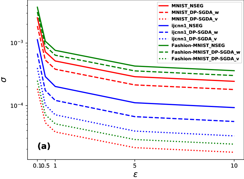
Figure 1: (a) Comparison of $\sigma$ for NSEG and DP-SGDA (Linear setting) on three datasets with different $\epsilon$ and $\delta$=1e-6. (b)Comparison of AUC performance for SGDA and DP-SGDA in MLP settings on three datasets with different hidden units and $\epsilon$=1 and $\delta$=1e-6. (c) Comparison of AUC performance for DP-SGDA (Linear and MLP settings) on three datasets with different batch size and $\epsilon$=1 and $\delta$=1e-6.

Privacy Budget Settings. In the experiments, we set up five privacy levels from small to large: $\epsilon\in\{0.1,0.5,1,5,10\}$. We also consider three different $\delta$ from $\{\mathrm{1e\!-\!4},\mathrm{1e\!-\!5},\mathrm{1e\!-\!6}\}$. Due to space limitation, we only report the performance when $\delta=\mathrm{1e\!-\!6}$. More results can be found in Appendix F. To estimate the Lipschitz constants $G_{\mathbf{w}}$ and $G_{\mathbf{v}}$ (in Theorem 1), we first run the algorithms without adding noise. Then we calculate the maximum gradient norms of AUC loss w.r.t $\mathbf{w}$ and $\mathbf{v}$ and assign them as $G_{\mathbf{w}}$ and $G_{\mathbf{v}}$, respectively. According to these parameters, we calculate the noise parameter $\sigma$ by applying autodp, which is widely used in the existing works [Wang et al., 2019b].

Compared Algorithms. Boob and Guzmán [2021] is the only existing paper that considers differential privacy in the convex-concave minimax problem. Therefore, we use their single-loop NSEG algorithm as our baseline method on the AUC optimization under the linear setting.

4.2 Results

We report our evaluation and results on the utility and privacy trade-off of the DP-SGDA. Then we follow the experiment design by [Abadi et al., 2016] to study the effect of the parameters - hidden units and batch sizes.

General AUC Performance vs Privacy. The general performance of all algorithms under linear and MLP settings of AUC optimization is shown in Table 2. Since the standard deviation of the AUC performance is around $[0,0.1\%]$ and the difference between different algortihms is very small, we only report the average AUC performance. First, without adding noise into gradients, we can find the NSEG method and our DP-SGDA method have similar performance under the linear case. Furthermore, we can find the performance of the DP-SGDA with MLP model can outperform linear models on all datasets. This is because non-linear models have better expression power and therefore it can learn more information among features than linear models. Second, by adding noise into the gradients, we can find the AUC performance of all models is decreased on all datasets. However, by increasing the privacy budget $\epsilon$, the AUC performance is increased. The reason is that $\epsilon$ and $\sigma$ have opposite trends according to equation (3). The relation between $\epsilon$ and AUC score also verifies our Theorem 2 and Theorem 5. Third, to verify our statement in Remark 2, we compare the $\sigma$ values from NSEG and DP-SGDA on all datasets in Figure 1(a). From the figure, it is clear that the $\sigma$ from NSEG is larger than ours in all $\epsilon$ settings since it is calibrated based on the gradients’ sensitivity from both $\mathbf{w}$ and $\mathbf{v}$. In fact, the sensitivity w.r.t. $\mathbf{v}$ is small as it is a one-dimensional variable for AUC maximization. Therefore, NSEG leads to overestimate on the noise addition towards $\mathbf{v}$. From Table 2 we observe our DP-SGDA achieves better AUC score than NSEG under the same privacy budget.

Different Hidden Units. In DP-SGDA under the MLP setting, the hidden unit is one of the most important factors affecting the model performance. Therefore, we compare the AUC performance with respect to the different hidden units in Figure 1(b). If we provide a small number of hidden units, the model will suffer from poor generalization capability. Using a large number of hidden units will make the model easier to fit the training set. For SGDA (non-private) training, it is often helpful to apply a large number of hidden units, as long as the model does not overfit. In agreement with this intuition, we find the model performance improves with increasing hidden units in Figure 1(b). However, for DP-SGDA training, more hidden units increase the sensitivity of the gradients, which leads to more noise added at each update. Therefore, in contrast to the non-private setting, we find the AUC performance decreases when the number of hidden units increases.

Different Mini-Batch Size. From Theorem 1 and Theorem 3, we find mini-batch size can influence the Gaussian noise variances $\sigma_{\mathbf{w}}^{2}$ and $\sigma_{\mathbf{v}}^{2}$ as well as the convergence rate. Selecting the mini-batch size must balance two conflicting objectives. On one hand, a small mini-batch size may lead to sub-optimal performance. On the other hand, for large batch sizes, the added noise has a smaller relative effect. Therefore, we show the AUC score for DP-SGDA with different mini-batch sizes in Figure 1(c). The experimental results show that the mini-batch size has a relatively large impact on the AUC performance when the mini-batch size is small.

5 Conclusion

In this paper, we have used algorithmic stability to conduct utility analysis of the DP-SGDA algorithm for minimax problems under DP constraints. For the convex-concave setting, we proved that DP-SGDA can attain an optimal rate $\mathcal{O}(\frac{1}{\sqrt{n}}+\frac{\sqrt{d\log(1/\delta)}}{n\epsilon})$ in terms of the weak primal-dual population risk while providing $(\epsilon,\delta)$-DP for both smooth and nonsmooth cases. For the nonconvex-strongly-concave case, assuming that the empirical risk satisfies the PL condition we proved the excess primal population risk of DP-SGDA can achieve a utility bound $\mathcal{O}\bigl{(}\frac{1}{n^{1/3}}+\frac{\sqrt{d\log(1/\delta)}}{n^{5/6}\epsilon}\bigr{)}$. Experiments on three benchmark datasets illustrate the effectiveness of DP-SGDA.

For future work, it would be interesting to improve the utility bound for the nonconvex-strongly-convex setting. It also remains unclear to us how to establish the utility bound for DP-SGDA when gradient clipping techniques are enforced at each iteration. Finally, it would also be interesting to evaluate the performance of DP-SGDA on other motivating examples such as GAN, MDP and robust optimization.

Appendix for "Differentially Private SGDA for Minimax Problems"

Appendix A Motivating Examples

We provide several examples that can be formulated as a stochastic minimax problem. All these examples have corresponding empirical minimax formulations.

AUC Maximization. Area Under the ROC Curve (AUC) is a widely used measure for binary classification. Optimizing AUC with square loss can be formulated as

$$\min_{\theta\in\Theta}\mathbb{E}_{\mathbf{z},\mathbf{z}^{\prime}}[(1-h(\theta;\mathbf{x})+h(\theta;\mathbf{x}^{\prime}))^{2}|y=1,y^{\prime}=-1]$$

where $h:\Theta\times\mathbb{R}^{d}\rightarrow\mathbb{R}$ is the scoring function for the classifier. It has been shown this problem is equivalent to a minimax problem once auxiliary variables $a,b,\mathbf{v}\in\mathbb{R}$ are introduced [ying2016stochastic-supp].

$$\min_{\theta,a,b}\max_{\mathbf{v}}F(\theta,a,b,c)=\mathbb{E}_{\mathbf{z}}[f(\theta,a,b,\mathbf{v};\mathbf{z})]$$

where $f=(1-p)(h(\theta;\mathbf{x})-a)^{2}\mathbb{I}[y=1]+p(h(\theta;\mathbf{x})-b)^{2}\mathbb{I}[y=-1]+2(1+\mathbf{v})(ph(\theta;\mathbf{x})\mathbb{I}[y=-1]-(1-p)h(\theta;\mathbf{x})\mathbb{I}[y=1])]-p(1-p)\mathbf{v}^{2}$ and $p=\mathbb{P}[y=1]$. Such problem is (non)convex-concave. In particular, liu2019stochastic-supp showed that when $h$ is a one hidden layer neural network the objective $f$ satisfies the Polyak-Łojasiewicz condition. Differential privacy has been applied to learn private classifier by optimizing AUC [wang2021differentially-supp]. The proposed privacy mechanisms there are objective perturbation and output perturbation.

Generative Adversarial Networks (GANs). GAN is introduced in goodfellow2014generative-supp which can be regarded as a game between a generator network $G_{\mathbf{v}}$ and a discriminator network $D_{\mathbf{w}}$. The generator network produces synthetic data from random noise $\xi$, while the discriminator network discriminates between the true data and the synthetic data. In particular, a popular variant of GAN named as WGAN [arjovsky2017wasserstein-supp] can be written as a minimax problem

$$\min_{\mathbf{w}}\max_{\mathbf{v}}\mathbb{E}[f(\mathbf{w},\mathbf{v};\mathbf{z},\xi)]:=\mathbb{E}_{\mathbf{z}}[D_{\mathbf{w}}(\mathbf{z})]-\mathbb{E}_{\xi}[D_{\mathbf{w}}(G_{\mathbf{v}}(\xi))].$$

Recently sahiner2021hidden-supp showed that WGAN with a two-layer discriminator and generator can be expressed as a convex-concave problem. An heuristic differentially private version of RMSProp were employed to train GANs by xie2018differentially-supp. Recently differential privacy has successfully applied to private synthetic data generation by GAN framework [jordon2018pate-supp, beaulieu2019privacy-supp].

Markov Decision Process (MDP). Let $\mathcal{A}$ be a finite action space. For any $a\in\mathcal{A}$, $P(a)\in[0,1]^{n\times n}$ is the state-transition probability matrix and $\mathbf{r}(a)\in[0,1]^{n}$ is the vector of expected state-transition rewards. In the infinite-horizon average-reward Markov decision problem, one aims to find a stationary policy $\pi$ to make an infinite sequence of actions and optimize the average-per-time-step reward $\bar{v}$. By classical theory of dynamics programming [puterman2014markov-supp], finding an optimal policy is equivalent as solving the fixed-point Bellman equation

$$\bar{v}^{*}+h^{*}_{i}=\max_{a\in\mathcal{A}}\big{\{}\sum_{j=1}^{n}(p_{ij}(a)h^{*}_{i}+p_{ij}(a)r_{ij}(a))\big{\}},\quad\forall i$$

where $\mathbf{h}\in\mathbb{R}^{n}$ is the difference-of-value vector. wang2017primal-supp showed that this problem is equivalent to the minimax problem as follow

$$\min_{\mathbf{h}\in\mathcal{H}}\max_{\mu\in\mathcal{U}}\mu^{\top}((P(a)-I)\mathbf{h}+\mathbf{r}(a))$$

where $\mathcal{H}$ and $\mathcal{U}$ are the feasible regions chosen according to the mixing time and stationary distribution. We refer to zhang2021generalization-supp for a discussion on the measure of population risk.

Robust Optimization and Fairness. Let $\mathcal{D}_{1},\cdots,\mathcal{D}_{m}$ be $m$ different distributions on some support. The aim is to minimize the worst population risks $L$ parameterized by some $\mathbf{w}$ among multiple scenarios:

$$\min_{\mathbf{w}\in\mathcal{W}}L(\mathbf{w})=\max_{1\leq i\leq m}\big{\{}\mathbb{E}_{\mathbf{z}_{1}\sim\mathcal{D}_{1}}[\ell(\mathbf{w};\mathbf{z}_{1})],\cdots,\mathbb{E}_{\mathbf{z}_{m}\sim\mathcal{D}_{m}}[\ell(\mathbf{w};\mathbf{z}_{m})]\big{\}}$$

This problem can be reformulated as a zero-sum game between two players $\mathbf{w}$ and $\mathbf{v}$ as follow

$$\min_{\mathbf{w}\in\mathcal{W}}\max_{\mathbf{v}\in\Delta_{m}}\sum_{i=1}^{m}v_{i}\mathbb{E}_{\mathbf{z}_{i}\sim\mathcal{D}_{i}}[\ell(\mathbf{w};\mathbf{z}_{i})]=\mathbb{E}\Big{[}\sum_{i=1}^{m}v_{i}\ell(\mathbf{w};\mathbf{z}_{i})\Big{]}$$

where $\Delta_{m}=\bigl{\{}\mathbf{v}\in\mathbb{R}^{m}:v_{i}\geq 0,\sum_{i=1}^{m}v_{i}=1\bigr{\}}$ denotes the $m$-dimensional simplex. Such robust optimization formulation has been recently proposed to address fairness among subgroups [mohri2019agnostic-supp] and federated learning on heterogeneous populations [li2019fair-supp].

Appendix B Proofs of Theorem 1 and Remark 1

In this section, we prove the privacy guarantee of DP-SGDA based on the privacy-amplification by the subsampling result, which is a direct application of Theorem 1 in abadi2016deep-supp. First we introduce some necessary definitions.

Definition 6.

Given a function $g:\mathcal{Z}^{n}\rightarrow\mathbb{R}^{d}$, we say $g$ has $\Delta(g)$ $\ell_{2}$-sensitivity if for any neighboring datasets $S,S^{\prime}$ we have

$$\|g(S)-g(S^{\prime})\|_{2}\leq\Delta(g).$$

Definition 7 ([abadi2016deep-supp]).

For an (randomized) algorithm $A$, and neighboring datasets $S,S^{\prime}$ the $\lambda$-th moment is given as

$$\alpha_{A}(\lambda,S,S^{\prime})=\log\mathbb{E}_{O\sim A(S)}\Big{[}\Big{(}\frac{\mathbb{P}[A(S)=O]}{\mathbb{P}[A(S^{\prime})=O]}\Big{)}^{\lambda}\Big{]}.$$

The moments accountant is then defined as

$$\alpha_{A}(\lambda)=\sup_{S,S^{\prime}}\alpha_{A}(\lambda,S,S^{\prime}).$$

Lemma 1 ([abadi2016deep-supp]).

Consider a sequence of mechanisms $\{A_{t}\}_{t\in[T]}$ and the composite mechanism $A=(A_{1},\cdots,A_{T})$.

1. [Composability] For any $\lambda$,

   $$\alpha_{A}(\lambda)=\sum_{t=1}^{T}\alpha_{A_{t}}(\lambda).$$

2. [Tail bound] For any $\epsilon$, the mechanism $A$ is $(\epsilon,\delta)$ differentially private for

   $$\delta=\min_{\lambda}\alpha_{A}(\lambda)-\lambda\epsilon.$$

Lemma 2 ([abadi2016deep-supp]).

Consider a sequence of mechanisms $A_{t}=g_{t}(S_{t})+\xi_{t}$ where $\xi\sim\mathcal{N}(0,\sigma^{2}I)$. Here each function $g_{t}:\mathcal{Z}^{m}\rightarrow\mathbb{R}^{d}$ has $\ell_{2}$-sensitivity of $1$. And each $S_{t}$ is a subsample of size $m$ obtained by uniform sampling without replacement from $S$, i.e. $S_{t}\sim(Unif(S))^{m}$, Then

$$\alpha_{A}(\lambda)\leq\frac{m^{2}n\lambda(\lambda+1)}{n^{2}(n-m)\sigma^{2}}+\mathcal{O}(\frac{m^{3}\lambda^{3}}{n^{3}\sigma^{3}}).$$

Theorem 6 (Theorem 1 restated).

There exist constants $c_{1},c_{2}$ and $c_{3}$ so that for any $\epsilon<c_{1}T/n^{2}$, Algorithm 1 is $(\epsilon,\delta)$-differentially private for any $\delta>0$ if we choose

$$\sigma_{\mathbf{w}}\geq\frac{c_{2}G_{\mathbf{w}}\sqrt{T\log(1/\delta)}}{n\epsilon}\text{ and }\sigma_{\mathbf{v}}\geq\frac{c_{3}G_{\mathbf{v}}\sqrt{T\log(1/\delta)}}{n\epsilon}.$$

Proof.

Let $S=\{\mathbf{z}_{1},\cdots,\mathbf{z}_{n}\}$ and $S^{\prime}=\{\mathbf{z}^{\prime}_{1},\cdots,\mathbf{z}^{\prime}_{n}\}$ be two neighboring datasets. At iteration $t$, we first focus on $A_{t}^{\mathbf{w}}=\frac{1}{m}\sum_{j=1}^{m}\nabla_{\mathbf{w}}f(\mathbf{w}_{t},\mathbf{v}_{t};\mathbf{z}_{i_{t}^{j}})+\xi_{t}$. Since $f(\cdot,\mathbf{v};\mathbf{z})$ is $G_{\mathbf{w}}$-Lipschitz continuous, it implies for any neighboring datasets $S,S^{\prime}$,

$$\Big{\|}\frac{1}{m}\sum_{j=1}^{m}\nabla_{\mathbf{w}}f(\mathbf{w}_{t},\mathbf{v}_{t};\mathbf{z}_{i_{t}^{j}})-\frac{1}{m}\sum_{j=1}^{m}\nabla_{\mathbf{w}}f(\mathbf{w}_{t},\mathbf{v}_{t};\mathbf{z}^{\prime}_{i_{t}^{j}})\Big{\|}_{2}\leq\frac{2G_{\mathbf{w}}}{m}.$$

Therefore we can define $g_{t}(S_{t})=\frac{1}{2G_{\mathbf{w}}}\sum_{j=1}^{m}\nabla_{\mathbf{w}}f(\mathbf{w}_{t},\mathbf{v}_{t},\mathbf{z}_{i_{t}^{j}})$ such that $\Delta(g_{t})=1$. By Lemma a) b) and 2, the log moment of the composite mechanism $A^{\mathbf{w}}=(A_{1}^{\mathbf{w}},\cdots,A_{T}^{\mathbf{w}})$ can be bounded as follows

$$\alpha_{A^{\mathbf{w}}}(\lambda)\leq\frac{m^{2}T\lambda^{2}}{n^{2}\tilde{\sigma}_{\mathbf{w}}^{2}}.$$

where $\tilde{\sigma}_{\mathbf{w}}=\sigma_{\mathbf{w}}/2G_{\mathbf{w}}$. Similarly, since $A_{t}^{\mathbf{v}}=\nabla_{\mathbf{w}}f(\mathbf{w}_{t},\mathbf{v}_{t};\mathbf{z}_{i_{t}})+\zeta_{t}$ has $\ell_{2}$-sensitivity $2G_{\mathbf{v}}/m$, then the log moment of the final output $A=(A_{1}^{\mathbf{w}},A_{1}^{\mathbf{v}},\cdots,A_{T}^{\mathbf{w}},A_{T}^{\mathbf{v}})$ can be bounded as follows

$$\alpha_{A}(\lambda)\leq\alpha_{A^{\mathbf{v}}}(\lambda)+\alpha_{A^{\mathbf{w}}}(\lambda)\leq\frac{m^{2}T\lambda^{2}}{n^{2}\tilde{\sigma}_{\mathbf{w}}^{2}}+\frac{m^{2}T\lambda^{2}}{n^{2}\tilde{\sigma}_{\mathbf{v}}^{2}}.$$

By Lemma b) a), to guarantee $A$ to be $(\epsilon,\delta)$-differentially private, it suffices that

$$\frac{\lambda^{2}m^{2}T}{n^{2}\tilde{\sigma}_{\mathbf{w}}^{2}}\leq\frac{\lambda\epsilon}{4},\frac{\lambda^{2}m^{2}T}{n^{2}\tilde{\sigma}_{\mathbf{v}}^{2}}\leq\frac{\lambda\epsilon}{4},\exp(-\frac{\lambda\epsilon}{4})\leq\delta,\lambda\leq\tilde{\sigma}_{\mathbf{w}}^{2}\log(\frac{n}{m\tilde{\sigma}_{\mathbf{w}}})\text{ and }\lambda\leq\tilde{\sigma}_{\mathbf{v}}^{2}\log(\frac{n}{m\tilde{\sigma}_{\mathbf{v}}})$$

It is now easy to verify that when $\epsilon=c_{1}m^{2}T/n^{2}$, we can satisfy all these conditions by setting

$$\tilde{\sigma}_{\mathbf{w}}\geq\frac{c_{2}\sqrt{T\log(1/\delta)}}{n\epsilon}\text{ and }\tilde{\sigma}_{\mathbf{v}}\geq\frac{c_{3}\sqrt{T\log(1/\delta)}}{n\epsilon}$$

for some explicit constants $c_{1},c_{2}$ and $c_{3}$. The proof is complete. ∎

Proof of Remark 1.

Without loss of generality, we consider with only one $\sigma$ in the the proof of Theorem 1. Then algorithm $A$ is guaranteed to be $(\epsilon,\delta)$-DP if one can find $\lambda>0$ such that

$$\frac{\lambda^{2}m^{2}T}{n^{2}\sigma^{2}}\leq\frac{\lambda\epsilon}{2},\,\exp(-\frac{\lambda\epsilon}{2})\leq\delta,\text{ and }\lambda\leq\sigma^{2}\log(\frac{n}{m\sigma})$$

Given $\delta=\frac{1}{n^{2}}$, the second inequality can be reformulated as $\lambda\geq\frac{4\log(n)}{\epsilon}$. Therefore by choosing $\sigma^{2}=\frac{8m^{2}T\log(n)}{n^{2}\epsilon^{2}}$, the first inequality becomes $\lambda\leq\frac{4\log(n)}{\epsilon}$, indicating $\lambda=\frac{4\log(n)}{\epsilon}$. It suffices to show such choice of $\lambda$ satisfies the third inequality, which is straightforward by the choice of $m$ and $\epsilon\leq 1$. The proof is complete. ∎

Appendix C Proofs for the convex-concave setting in Section 3.1

Recall that the error decomposition (3.1) given in Section 3.1 that the weak PD risk can be decomposed as follows:

$$\triangle^{w}(\bar{\mathbf{w}}_{T},\bar{\mathbf{v}}_{T})=\triangle^{w}(\bar{\mathbf{w}}_{T},\bar{\mathbf{v}}_{T})-\triangle^{w}_{S}(\bar{\mathbf{w}}_{T},\bar{\mathbf{v}}_{T})+\triangle^{w}_{S}(\bar{\mathbf{w}}_{T},\bar{\mathbf{v}}_{T}),$$ (6)

where the term $\triangle^{w}(\bar{\mathbf{w}}_{T},\bar{\mathbf{v}}_{T})-\triangle^{w}_{S}(\bar{\mathbf{w}}_{T},\bar{\mathbf{v}}_{T})$ is the generalization error and the term $\triangle^{w}_{S}(\bar{\mathbf{w}}_{T},\bar{\mathbf{v}}_{T})$ is the optimization error.

The proof of Theorem 2 involves the estimation of the optimization error and generalization error which are performed in the subsequent subsection, respectively.

C.1 Estimation of Optimization Error

We start by studying the optimization error for Algorithm 1. This is obtained as a direct corollary of nemirovski2009robust-supp, with the existence of the Gaussian noise’s variance and the mini-batch. Recall that $d=\max\{d_{1},d_{2}\}.$

Lemma 3.

Suppose (A1) holds, and $F_{S}$ is convex-concave. Let the stepsizes $\eta_{\mathbf{w},t}=\eta_{\mathbf{v},t}=\eta$, $t\in[T]$ for some $\eta>0$. Then Algorithm 1 satisfies

$$\sup_{\mathbf{v}\in\mathcal{V}}\mathbb{E}_{A}[F_{S}(\bar{\mathbf{w}}_{T},\mathbf{v})]-\inf_{\mathbf{w}\in\mathcal{W}}\mathbb{E}_{A}[F_{S}(\mathbf{w},\bar{\mathbf{v}}_{T})]\leq\frac{\eta(G_{\mathbf{w}}^{2}+G_{\mathbf{v}}^{2})}{2}+\frac{D_{\mathbf{w}}^{2}+D_{\mathbf{v}}^{2}}{\eta T}+\frac{(D_{\mathbf{w}}G_{\mathbf{w}}+D_{\mathbf{v}}G_{\mathbf{v}})}{\sqrt{mT}}+\eta d(\sigma_{\mathbf{w}}^{2}+\sigma_{\mathbf{v}}^{2}).$$

Proof.

According to the non-expansiveness of projection and update rule of Algorithm 1, for any $\mathbf{w}\in\mathcal{W}$, we have

$$\|\mathbf{w}_{t+1}-\mathbf{w}\|_{2}^{2}\leq\Big{\|}\mathbf{w}_{t}-\mathbf{w}-\frac{\eta}{m}\sum_{j=1}^{m}\nabla_{\mathbf{w}}f(\mathbf{w}_{t},\mathbf{v}_{t};\mathbf{z}_{i_{t}^{j}})-\eta\xi_{t}\Big{\|}_{2}^{2}$$

$$\leq \|\mathbf{w}_{t}-\mathbf{w}\|_{2}^{2}+2\eta\Big{\langle}\mathbf{w}-\mathbf{w}_{t},\frac{1}{m}\sum_{j=1}^{m}\nabla_{\mathbf{w}}f(\mathbf{w}_{t},\mathbf{v}_{t};\mathbf{z}_{i_{t}^{j}})+\xi_{t}\Big{\rangle}+\eta^{2}\Big{\|}\frac{1}{m}\sum_{j=1}^{m}\nabla_{\mathbf{w}}f(\mathbf{w}_{t},\mathbf{v}_{t};\mathbf{z}_{i_{t}^{j}})\Big{\|}_{2}^{2}+\eta^{2}\|\xi_{t}\|_{2}^{2}$$

$$+2\eta^{2}\Big{\langle}\frac{1}{m}\sum_{j=1}^{m}\nabla_{\mathbf{w}}f(\mathbf{w}_{t},\mathbf{v}_{t};\mathbf{z}_{i_{t}^{j}}),\xi_{t}\Big{\rangle}$$

$$\leq \|\mathbf{w}_{t}-\mathbf{w}\|_{2}^{2}+2\eta\langle\mathbf{w}-\mathbf{w}_{t},\nabla_{\mathbf{w}}F_{S}(\mathbf{w}_{t},\mathbf{v}_{t})\rangle+2\eta\Big{\langle}\mathbf{w}-\mathbf{w}_{t},\frac{1}{m}\sum_{j=1}^{m}\nabla_{\mathbf{w}}f(\mathbf{w}_{t},\mathbf{v}_{t};\mathbf{z}_{i_{t}^{j}})-\nabla_{\mathbf{w}}F_{S}(\mathbf{w}_{t},\mathbf{v}_{t})\Big{\rangle}$$

$$+\eta^{2}G_{\mathbf{w}}^{2}+\eta^{2}\|\xi_{t}\|_{2}^{2}+2\eta^{2}\Big{\langle}\frac{1}{m}\sum_{j=1}^{m}\nabla_{\mathbf{w}}f(\mathbf{w}_{t},\mathbf{v}_{t};\mathbf{z}_{i_{t}^{j}}),\xi_{t}\Big{\rangle}+2\eta\langle\mathbf{w}-\mathbf{w}_{t},\xi_{t}\rangle,$$

where in the last inequality we have used $f(\cdot,\mathbf{v}_{t},\mathbf{z}_{i_{t}^{j}})$ is $G_{\mathbf{w}}$-Lipschitz continuous. According to the convexity of $F_{S}(\cdot,\mathbf{v}_{t})$ we know

$$2\eta(F_{S}(\mathbf{w}_{t},\mathbf{v}_{t})\!-\!F_{S}(\mathbf{w},\mathbf{v}_{t}))\leq \|\mathbf{w}_{t}\!-\!\mathbf{w}\|_{2}^{2}\!-\!\|\mathbf{w}_{t+1}\!-\!\mathbf{w}\|_{2}^{2}\!+\!2\eta\Big{\langle}\mathbf{w}\!-\!\mathbf{w}_{t},\frac{1}{m}\sum_{j=1}^{m}\nabla_{\mathbf{w}}f(\mathbf{w}_{t},\mathbf{v}_{t};\mathbf{z}_{i_{t}^{j}})\!-\!\nabla_{\mathbf{w}}F_{S}(\mathbf{w}_{t},\mathbf{v}_{t})\Big{\rangle}$$

$$+\eta^{2}G_{\mathbf{w}}^{2}+\eta^{2}\|\xi_{t}\|_{2}^{2}+2\eta^{2}\Big{\langle}\frac{1}{m}\sum_{j=1}^{m}\nabla_{\mathbf{w}}f(\mathbf{w}_{t},\mathbf{v}_{t};\mathbf{z}_{i_{t}^{j}}),\xi_{t}\Big{\rangle}+2\eta\langle\mathbf{w}-\mathbf{w}_{t},\xi_{t}\rangle.$$

Taking a summation of the above inequality from $t=1$ to $T$ we derive

$$2\eta\sum_{t=1}^{T}(F_{S}(\mathbf{w}_{t},\mathbf{v}_{t})-F_{S}(\mathbf{w},\mathbf{v}_{t}))\leq\|\mathbf{w}_{1}-\mathbf{w}\|_{2}^{2}+2\eta\sum_{t=1}^{T}\Big{\langle}\mathbf{w}-\mathbf{w}_{t},\frac{1}{m}\sum_{j=1}^{m}\nabla_{\mathbf{w}}f(\mathbf{w}_{t},\mathbf{v}_{t};\mathbf{z}_{i_{t}^{j}})-\nabla_{\mathbf{w}}F_{S}(\mathbf{w}_{t},\mathbf{v}_{t})\Big{\rangle}\\ +T\eta^{2}G_{\mathbf{w}}^{2}+\eta^{2}\sum_{t=1}^{T}\|\xi_{t}\|_{2}^{2}+2\eta^{2}\sum_{t=1}^{T}\Big{\langle}\frac{1}{m}\sum_{j=1}^{m}\nabla_{\mathbf{w}}f(\mathbf{w}_{t},\mathbf{v}_{t};\mathbf{z}_{i_{t}^{j}}),\xi_{t}\Big{\rangle}+2\eta\langle\mathbf{w}-\mathbf{w}_{t},\xi_{t}\rangle.$$

It then follows from the concavity of $F_{S}(\mathbf{w},\cdot)$ and Schwartz’s inequality that

$$2\sum_{t=1}^{T}\eta(F_{S}(\mathbf{w}_{t},\mathbf{v}_{t})-F_{S}(\mathbf{w},\bar{\mathbf{v}}_{T}))\leq 2D_{\mathbf{w}}^{2}-2\eta\sum_{t=1}^{T}\Big{\langle}\mathbf{w}_{t},\frac{1}{m}\sum_{j=1}^{m}\nabla_{\mathbf{w}}f(\mathbf{w}_{t},\mathbf{v}_{t};\mathbf{z}_{i_{t}^{j}})-\nabla_{\mathbf{w}}F_{S}(\mathbf{w}_{t},\mathbf{v}_{t})\Big{\rangle}\\ +2D_{\mathbf{w}}\eta\Big{\|}\sum_{t=1}^{T}(\frac{1}{m}\sum_{j=1}^{m}\nabla_{\mathbf{w}}f(\mathbf{w}_{t},\mathbf{v}_{t};\mathbf{z}_{i_{t}^{j}})-\nabla_{\mathbf{w}}F_{S}(\mathbf{w}_{t},\mathbf{v}_{t})\Big{\|}_{2}\\ +T\eta^{2}G_{\mathbf{w}}^{2}+\eta^{2}\sum_{t=1}^{T}\|\xi_{t}\|_{2}^{2}+2\eta^{2}\sum_{t=1}^{T}\Big{\langle}\frac{1}{m}\sum_{j=1}^{m}\nabla_{\mathbf{w}}f(\mathbf{w}_{t},\mathbf{v}_{t};\mathbf{z}_{i_{t}^{j}}),\xi_{t}\Big{\rangle}+2\eta\langle\mathbf{w}-\mathbf{w}_{t},\xi_{t}\rangle.$$

We can take expectations on the randomness of $A$ over both sides of(C.1) and get

$$2\eta\sum_{t=1}^{T}\mathbb{E}_{A}[F_{S}(\mathbf{w}_{t},\mathbf{v}_{t})\!-\!F_{S}(\mathbf{w},\bar{\mathbf{v}}_{T})]\leq 2D_{\mathbf{w}}^{2}\!+\!2D_{\mathbf{w}}\eta\mathbb{E}_{A}\Big{[}\Big{\|}\sum_{t=1}^{T}\frac{1}{m}\sum_{j=1}^{m}\nabla_{\mathbf{w}}f(\mathbf{w}_{t},\mathbf{v}_{t};\mathbf{z}_{i_{t}^{j}})\!-\!\nabla_{\mathbf{w}}F_{S}(\mathbf{w}_{t},\mathbf{v}_{t})\Big{\|}_{2}\Big{]}$$

$$+T\eta^{2}G_{\mathbf{w}}^{2}+\eta^{2}d_{1}\sigma_{\mathbf{w}}^{2},$$

where we used that the variance $\mathbb{E}_{A}[\|\xi_{t}\|_{2}^{2}]=d_{1}\sigma_{\mathbf{w}}^{2}$, the unbiasedness $\mathbb{E}_{A}[\langle\mathbf{w}_{t},\frac{1}{m}\sum_{j=1}^{m}\nabla_{\mathbf{w}}f(\mathbf{w}_{t},\mathbf{v}_{t};\mathbf{z}_{i_{t}^{j}})-\nabla_{\mathbf{w}}F_{S}(\mathbf{w}_{t},\mathbf{v}_{t})\rangle]=0$, the independence $\mathbb{E}_{A}[\langle\frac{1}{m}\sum_{j=1}^{m}\nabla_{\mathbf{w}}f(\mathbf{w}_{t},\mathbf{v}_{t};\mathbf{z}_{i_{t}^{j}}),\xi_{t}\rangle]=0$ and $\mathbb{E}_{A}[\langle\mathbf{w}-\mathbf{w}_{t},\xi_{t}\rangle]=0$. Since the above inequality holds for all $\mathbf{w}$, we further get

$$2\eta\sum_{t=1}^{T}\mathbb{E}_{A}[F_{S}(\mathbf{w}_{t},\mathbf{v}_{t})]\!-\!\inf_{\mathbf{w}\in\mathcal{W}}\mathbb{E}_{A}[F_{S}(\mathbf{w},\bar{\mathbf{v}}_{T})]\leq 2D_{\mathbf{w}}^{2}\!+\!2D_{\mathbf{w}}\eta\mathbb{E}_{A}\Big{[}\Big{\|}\sum_{t=1}^{T}\frac{1}{m}\sum_{j=1}^{m}\nabla_{\mathbf{w}}f(\mathbf{w}_{t},\mathbf{v}_{t};\mathbf{z}_{i_{t}^{j}})\!-\!\nabla_{\mathbf{w}}F_{S}(\mathbf{w}_{t},\mathbf{v}_{t})\Big{\|}_{2}\Big{]}$$

$$+T\eta^{2}G_{\mathbf{w}}^{2}+\eta^{2}d_{1}\sigma_{\mathbf{w}}^{2},$$ (8)

According to Jensen’s inequality and $G_{\mathbf{w}}$-Lipschitz continuity we further derive

$$\Big{(}\mathbb{E}_{A}\Big{[}\Big{\|}\sum_{t=1}^{T}(\frac{1}{m}\sum_{j=1}^{m}\nabla_{\mathbf{w}}f(\mathbf{w}_{t},\mathbf{v}_{t};\mathbf{z}_{i_{t}^{j}})\!-\!\nabla_{\mathbf{w}}F_{S}(\mathbf{w}_{t},\mathbf{v}_{t})\Big{\|}_{2})\Big{]}\Big{)}^{2}$$

$$\leq \mathbb{E}_{A}\Big{[}\Big{\|}\sum_{t=1}^{T}(\frac{1}{m}\sum_{j=1}^{m}\nabla_{\mathbf{w}}f(\mathbf{w}_{t},\mathbf{v}_{t};\mathbf{z}_{i_{t}^{j}})\!-\!\nabla_{\mathbf{w}}F_{S}(\mathbf{w}_{t},\mathbf{v}_{t}))\Big{\|}_{2}^{2}\Big{]}=\sum_{t=1}^{T}\mathbb{E}_{A}\Big{[}\Big{\|}\frac{1}{m}\sum_{j=1}^{m}\nabla_{\mathbf{w}}f(\mathbf{w}_{t},\mathbf{v}_{t};\mathbf{z}_{i_{t}^{j}})-\nabla_{\mathbf{w}}F_{S}(\mathbf{w}_{t},\mathbf{v}_{t})\Big{\|}_{2}^{2}\Big{]}$$

$$\leq \frac{TG_{\mathbf{w}}^{2}}{m}.$$

Plugging the above estimate into (C.1) we arrive

$$2\eta\sum_{t=1}^{T}\mathbb{E}_{A}[F_{S}(\mathbf{w}_{t},\mathbf{v}_{t})]-\inf_{\mathbf{w}\in\mathcal{W}}\mathbb{E}_{A}[F_{S}(\mathbf{w},\bar{\mathbf{v}}_{T})]\leq 2D_{\mathbf{w}}^{2}+\frac{2D_{\mathbf{w}}\eta G_{\mathbf{w}}\sqrt{T}}{\sqrt{m}}+T\eta^{2}G_{\mathbf{w}}^{2}+T\eta^{2}d_{1}\sigma_{\mathbf{w}}^{2}.$$

By dividing $2\eta T$ on both sides we have

$$\frac{1}{T}\sum_{t=1}^{T}\mathbb{E}_{A}[F_{S}(\mathbf{w}_{t},\mathbf{v}_{t})]-\inf_{\mathbf{w}\in\mathcal{W}}\mathbb{E}_{A}[F_{S}(\mathbf{w},\bar{\mathbf{v}}_{T})]\leq\frac{D_{\mathbf{w}}^{2}}{\eta T}+\frac{D_{\mathbf{w}}G_{\mathbf{w}}}{\sqrt{mT}}+\frac{\eta G^{2}_{\mathbf{w}}}{2}+\frac{\eta d_{1}\sigma_{\mathbf{w}}^{2}}{2}.$$ (9)

In a similar way, we can show that

$$\frac{1}{T}\sum_{t=1}^{T}\sup_{\mathbf{v}\in\mathcal{V}}\mathbb{E}_{A}[F_{S}(\bar{\mathbf{w}}_{T},\mathbf{v})]-\mathbb{E}_{A}[F_{S}(\mathbf{w}_{t},\mathbf{v}_{t})]\leq\frac{D_{\mathbf{v}}^{2}}{\eta T}+\frac{D_{\mathbf{v}}G_{\mathbf{v}}}{\sqrt{mT}}+\frac{\eta G_{\mathbf{v}}^{2}}{2}+\frac{\eta d_{2}\sigma_{\mathbf{v}}^{2}}{2}.$$ (10)

The stated bound then follows from (9) and (10) and the fact that $d=\max\{d_{1},d_{2}\}.$ ∎

C.2 Estimation of Generalization Error

Next we move on to the generalization error. Firstly, we introduce a lemma that bridges the generalization and the stability. We say the randomized algorithm $A$ is $\varepsilon$-weakly-stable if, for any neighboring datasets $S,S^{\prime}$, there holds

$$\sup_{\mathbf{z}}\Big{(}\sup_{\mathbf{v}\in\mathcal{V}}\mathbb{E}_{A}[f(A_{\mathbf{w}}(S),\mathbf{v};\mathbf{z})-f(A_{\mathbf{w}}(S^{\prime}),\mathbf{v};\mathbf{z})]+\sup_{\mathbf{w}\in\mathcal{W}}\mathbb{E}_{A}[f(\mathbf{w},A_{\mathbf{v}}(S);\mathbf{z})-f(\mathbf{w},A_{\mathbf{v}}(S^{\prime});\mathbf{z})]\Big{)}\leq\varepsilon.$$

Lemma 4.

[lei2021stability-supp] If $A$ is $\varepsilon$-weakly-stable, then there holds

$$\triangle^{w}(A_{\mathbf{w}}(S),A_{\mathbf{v}}(S))-\triangle^{w}_{S}(A_{\mathbf{w}}(S),A_{\mathbf{v}}(S))\leq\varepsilon.$$

We also need the following standard lemma before we prove the stability of DP-SGDA.

Lemma 5 ([rockafellar1976monotone-supp]).

Let $f$ be a convex-concave function. Then

$$\left\langle\begin{pmatrix}\mathbf{w}-\mathbf{w}^{\prime}\\ \mathbf{v}-\mathbf{v}^{\prime}\end{pmatrix},\begin{pmatrix}\nabla_{\mathbf{w}}f(\mathbf{w},\mathbf{v})-\nabla_{\mathbf{w}}f(\mathbf{w}^{\prime},\mathbf{v}^{\prime})\\ \nabla_{\mathbf{v}}f(\mathbf{w}^{\prime},\mathbf{v}^{\prime})-\nabla_{\mathbf{v}}f(\mathbf{w},\mathbf{v})\end{pmatrix}\right\rangle\geq 0.$$

The stability analysis is given in the following lemma. This lemma is an extension of the uniform argument stability results in lei2021stability-supp to the case of mini-batch DP-SGDA.

Lemma 6.

Suppose the function $F_{S}$ is convex-concave. Let the stepsizes $\eta_{\mathbf{w},t}=\eta_{\mathbf{v},t}=\eta$ for some $\eta>0$.

1. Assume (A1) and (A3) hold, then Algorithm 1 satisfies

   $$\triangle^{w}(\bar{\mathbf{w}}_{T},\bar{\mathbf{v}}_{T})-\triangle^{w}_{S}(\bar{\mathbf{w}}_{T},\bar{\mathbf{v}}_{T})\leq\frac{4\sqrt{e(T+T^{2}/n)}(G_{\mathbf{w}}+G_{\mathbf{v}})^{2}\eta\exp(L^{2}T\eta^{2}/2)}{\sqrt{n}}.$$

2. Assume (A1) holds, then Algorithm 1 satisfies

   $$\triangle^{w}(\bar{\mathbf{w}}_{T},\bar{\mathbf{v}}_{T})-\triangle^{w}_{S}(\bar{\mathbf{w}}_{T},\bar{\mathbf{v}}_{T})\leq 4\sqrt{2}\eta(G_{\mathbf{w}}+G_{\mathbf{v}})^{2}\Big{(}\sqrt{T}+\frac{T}{n}\Big{)}.$$

Proof.

Without loss of generality, let $S=\{\mathbf{z}_{1},\cdots,\mathbf{z}_{n}\},S^{\prime}=\{\mathbf{z}_{1}^{\prime},\cdots,\mathbf{z}_{n}^{\prime}\}$ be neighboring datasets differing by the last element, i.e. $\mathbf{z}_{n}\neq\mathbf{z}^{\prime}_{n}$. Let $\{\mathbf{w}_{t},\mathbf{v}_{t}\},\{\mathbf{w}_{t}^{\prime},\mathbf{v}_{t}^{\prime}\}$ be the sequence produced by Algorithm 1 w.r.t. $S$ and $S^{\prime}$, respectively. We first prove Part a). In the case $n\not\in I_{t}$, by the non-expansiveness of projection, we have

$$\left\|\begin{pmatrix}\mathbf{w}_{t+1}-\mathbf{w}_{t+1}^{\prime}\\ \mathbf{v}_{t+1}-\mathbf{v}_{t+1}^{\prime}\end{pmatrix}\right\|_{2}^{2}\leq\left\|\begin{pmatrix}\mathbf{w}_{t}-\frac{\eta}{m}\sum_{j=1}^{m}\nabla_{\mathbf{w}}f(\mathbf{w}_{t},\mathbf{v}_{t};z_{i_{t}^{j}})-\eta\xi_{t}-\mathbf{w}_{t}^{\prime}+\frac{\eta}{m}\sum_{j=1}^{m}\nabla_{\mathbf{w}}f(\mathbf{w}_{t}^{\prime},\mathbf{v}^{\prime}_{t};z_{i_{t}^{j}})+\eta\xi_{t}\\ \mathbf{v}_{t}+\frac{\eta}{m}\sum_{j=1}^{m}\nabla_{\mathbf{v}}f(\mathbf{w}_{t},\mathbf{v}_{t};z_{i_{t}^{j}})+\eta\zeta_{t}-\mathbf{v}_{t}^{\prime}-\frac{\eta}{m}\sum_{j=1}^{m}\nabla_{\mathbf{v}}f(\mathbf{w}_{t}^{\prime},\mathbf{v}^{\prime}_{t};z_{i_{t}^{j}})-\eta\zeta_{t}\end{pmatrix}\right\|_{2}^{2}$$

$$=\left\|\begin{pmatrix}\mathbf{w}_{t}-\mathbf{w}_{t}^{\prime}\\ \mathbf{v}_{t}-\mathbf{v}_{t}^{\prime}\end{pmatrix}\right\|_{2}^{2}+\frac{\eta}{m}\sum_{j=1}^{m}\left\langle\begin{pmatrix}\mathbf{w}_{t}-\mathbf{w}^{\prime}_{t}\\ \mathbf{v}_{t}-\mathbf{v}^{\prime}_{t}\end{pmatrix},\begin{pmatrix}\nabla_{\mathbf{w}}f(\mathbf{w}_{t},\mathbf{v}_{t};z_{i_{t}^{j}})-\nabla_{\mathbf{w}}f(\mathbf{w}_{t}^{\prime},\mathbf{v}^{\prime}_{t};z_{i_{t}^{j}})\\ \nabla_{\mathbf{v}}f(\mathbf{w}^{\prime}_{t},\mathbf{v}^{\prime}_{t};z_{i_{t}^{j}})-\nabla_{\mathbf{v}}f(\mathbf{w}_{t},\mathbf{v}_{t};z_{i_{t}^{j}})\end{pmatrix}\right\rangle$$

$$+\left\|\begin{pmatrix}\frac{\eta}{m}\sum_{j=1}^{m}(\nabla_{\mathbf{w}}f(\mathbf{w}_{t},\mathbf{v}_{t};z_{n})-\nabla_{\mathbf{w}}f(\mathbf{w}_{t}^{\prime},\mathbf{v}^{\prime}_{t};z^{\prime}_{n}))\\ \frac{\eta}{m}\sum_{j=1}^{m}(\nabla_{\mathbf{v}}f(\mathbf{w}_{t},\mathbf{v}_{t};z_{n})-\nabla_{\mathbf{v}}f(\mathbf{w}_{t}^{\prime},\mathbf{v}^{\prime}_{t};z^{\prime}_{n}))\end{pmatrix}\right\|_{2}^{2}$$

$$\leq(1+L^{2}\eta^{2})\left\|\begin{pmatrix}\mathbf{w}_{t}-\mathbf{w}_{t}^{\prime}\\ \mathbf{v}_{t}-\mathbf{v}_{t}^{\prime}\end{pmatrix}\right\|_{2}^{2},$$

where the last inequality follows from Lemma 5 and the $L$-smoothness assumption. If $n\in I_{t}$, then it follows that

$$\left\|\begin{pmatrix}\mathbf{w}_{t+1}-\mathbf{w}_{t+1}^{\prime}\\ \mathbf{v}_{t+1}-\mathbf{v}_{t+1}^{\prime}\end{pmatrix}\right\|_{2}^{2}\leq\left\|\begin{pmatrix}\mathbf{w}_{t}-\frac{\eta}{m}\sum_{j=1}^{m}\nabla_{\mathbf{w}}f(\mathbf{w}_{t},\mathbf{v}_{t};z_{i_{t}^{j}})-\eta\xi_{t}-\mathbf{w}_{t}^{\prime}+\frac{\eta}{m}\sum_{j=1}^{m}\nabla_{\mathbf{w}}f(\mathbf{w}_{t}^{\prime},\mathbf{v}^{\prime}_{t};z^{\prime}_{i_{t}^{j}})+\eta\xi_{t}\\ \mathbf{v}_{t}+\frac{\eta}{m}\sum_{j=1}^{m}\nabla_{\mathbf{v}}f(\mathbf{w}_{t},\mathbf{v}_{t};z_{i_{t}^{j}})+\eta\zeta_{t}-\mathbf{v}_{t}^{\prime}-\frac{\eta}{m}\sum_{j=1}^{m}\nabla_{\mathbf{v}}f(\mathbf{w}_{t}^{\prime},\mathbf{v}^{\prime}_{t};z^{\prime}_{i_{t}^{j}})-\eta\zeta_{t}\end{pmatrix}\right\|_{2}^{2}$$

$$\leq\frac{1}{m}\sum_{i_{t}^{j}\in I_{t},i_{t}^{j}\neq n}\left\|\begin{pmatrix}\mathbf{w}_{t}-\eta\nabla_{\mathbf{w}}f(\mathbf{w}_{t},\mathbf{v}_{t};z_{i_{t}^{j}})-\mathbf{w}_{t}^{\prime}+\eta\nabla_{\mathbf{w}}f(\mathbf{w}_{t}^{\prime},\mathbf{v}^{\prime}_{t};z^{\prime}_{i_{t}^{j}})\\ \mathbf{v}_{t}+\eta\nabla_{\mathbf{v}}f(\mathbf{w}_{t},\mathbf{v}_{t};z_{i_{t}^{j}})-\mathbf{v}_{t}^{\prime}-\eta\nabla_{\mathbf{v}}f(\mathbf{w}_{t}^{\prime},\mathbf{v}^{\prime}_{t};z^{\prime}_{i_{t}^{j}})\end{pmatrix}\right\|_{2}^{2}$$

$$+\frac{1}{m}\left\|\begin{pmatrix}\mathbf{w}_{t}-\eta\nabla_{\mathbf{w}}f(\mathbf{w}_{t},\mathbf{v}_{t};z_{n})-\mathbf{w}_{t}^{\prime}+\eta\nabla_{\mathbf{w}}f(\mathbf{w}_{t}^{\prime},\mathbf{v}^{\prime}_{t};z^{\prime}_{n})\\ \mathbf{v}_{t}+\eta\nabla_{\mathbf{v}}f(\mathbf{w}_{t},\mathbf{v}_{t};z_{n})-\mathbf{v}_{t}^{\prime}-\eta\nabla_{\mathbf{v}}f(\mathbf{w}_{t}^{\prime},\mathbf{v}^{\prime}_{t};z^{\prime}_{n})\end{pmatrix}\right\|_{2}^{2}$$

$$\leq\frac{m-1}{m}(1+L^{2}\eta^{2})\left\|\begin{pmatrix}\mathbf{w}_{t}-\mathbf{w}_{t}^{\prime}\\ \mathbf{v}_{t}-\mathbf{v}_{t}^{\prime}\end{pmatrix}\right\|_{2}^{2}+\frac{1+p}{m}\left\|\begin{pmatrix}\mathbf{w}_{t}-\mathbf{w}_{t}^{\prime}\\ \mathbf{v}_{t}-\mathbf{v}_{t}^{\prime}\end{pmatrix}\right\|_{2}^{2}$$

$$+\frac{1+1/p}{m}\eta^{2}\left\|\begin{pmatrix}\nabla_{\mathbf{w}}f(\mathbf{w}_{t},\mathbf{v}_{t};z_{n})-\nabla_{\mathbf{w}}f(\mathbf{w}_{t}^{\prime},\mathbf{v}_{t}^{\prime};z^{\prime}_{n})\\ \nabla_{\mathbf{v}}f(\mathbf{w}_{t},\mathbf{v}_{t};z_{n})-\nabla_{\mathbf{v}}f(\mathbf{w}_{t}^{\prime},\mathbf{v}_{t}^{\prime};z^{\prime}_{n})\end{pmatrix}\right\|_{2}^{2},$$ (11)

where in the last inequality we used the elementary inequality $(a+b)^{2}\leq(1+p)a^{2}+(1+1/p)b^{2}$ ($p>0$). Since $I_{t}$ are drawn uniformly at random with replacement, the event $n\not\in I_{t}$ happens with probability $1-m/n$ and the event $n\in I_{t}$ happens with probability $m/n$. Therefore, we know

$$\mathbb{E}_{i_{t}}\left[\left\|\begin{pmatrix}\mathbf{w}_{t+1}-\mathbf{w}_{t+1}^{\prime}\\ \mathbf{v}_{t+1}-\mathbf{v}_{t+1}^{\prime}\end{pmatrix}\right\|_{2}^{2}\right] \leq\frac{(n-m)(1+L^{2}\eta^{2})}{n}\left\|\begin{pmatrix}\mathbf{w}_{t}-\mathbf{w}_{t}^{\prime}\\ \mathbf{v}_{t}-\mathbf{v}_{t}^{\prime}\end{pmatrix}\right\|_{2}^{2}+\frac{m(1+L^{2}\eta^{2})}{n}\frac{m-1}{m}\left\|\begin{pmatrix}\mathbf{w}_{t}-\mathbf{w}_{t}^{\prime}\\ \mathbf{v}_{t}-\mathbf{v}_{t}^{\prime}\end{pmatrix}\right\|_{2}^{2}$$

$$+\frac{m}{n}\frac{1+p}{m}\left\|\begin{pmatrix}\mathbf{w}_{t}-\mathbf{w}_{t}^{\prime}\\ \mathbf{v}_{t}-\mathbf{v}_{t}^{\prime}\end{pmatrix}\right\|_{2}^{2}+\frac{m}{n}\frac{4(1+1/p)}{m}\eta^{2}(G_{\mathbf{w}}^{2}+G_{\mathbf{v}}^{2})$$

$$\leq\Big{(}1+L^{2}\eta^{2}+p/n\Big{)}\left\|\begin{pmatrix}\mathbf{w}_{t}-\mathbf{w}_{t}^{\prime}\\ \mathbf{v}_{t}-\mathbf{v}_{t}^{\prime}\end{pmatrix}\right\|_{2}^{2}+\frac{4(1+1/p)}{n}\eta^{2}(G_{\mathbf{w}}^{2}+G_{\mathbf{v}}^{2}).$$

Applying this inequality recursively, we derive

$$\mathbb{E}_{A}\left[\left\|\begin{pmatrix}\mathbf{w}_{t+1}-\mathbf{w}_{t+1}^{\prime}\\ \mathbf{v}_{t+1}-\mathbf{v}_{t+1}^{\prime}\end{pmatrix}\right\|_{2}^{2}\right]\leq\frac{4(1+1/p)}{n}(G_{\mathbf{w}}^{2}+G_{\mathbf{v}}^{2})\sum_{k=1}^{t}\eta^{2}\prod_{j=k+1}^{t}\Big{(}1+L^{2}\eta^{2}+p/n\Big{)}.$$

By the elementary inequality $1+a\leq\exp(a)$, we further derive

$$\mathbb{E}_{A}\left[\left\|\begin{pmatrix}\mathbf{w}_{t+1}-\mathbf{w}_{t+1}^{\prime}\\ \mathbf{v}_{t+1}-\mathbf{v}_{t+1}^{\prime}\end{pmatrix}\right\|_{2}^{2}\right] \leq\frac{4(1+1/p)}{n}(G_{\mathbf{w}}^{2}+G_{\mathbf{v}}^{2})\sum_{k=1}^{t}\eta^{2}\prod_{j=k+1}^{t}\exp\Big{(}L^{2}\eta^{2}+p/n\Big{)}$$

$$=\frac{4(1+1/p)}{n}(G_{\mathbf{w}}^{2}+G_{\mathbf{v}}^{2})\sum_{k=1}^{t}\eta^{2}\exp\Big{(}L^{2}\sum_{j=k+1}^{t}\eta^{2}+p(t-k)/n\Big{)}$$

$$\leq\frac{4(1+1/p)}{n}(G_{\mathbf{w}}^{2}+G_{\mathbf{v}}^{2})\exp\Big{(}L^{2}\sum_{j=1}^{t}\eta^{2}+pt/n\Big{)}\sum_{k=1}^{t}\eta^{2}.$$

By taking $p=n/t$ we get

$$\mathbb{E}_{A}\left[\left\|\begin{pmatrix}\mathbf{w}_{t+1}-\mathbf{w}_{t+1}^{\prime}\\ \mathbf{v}_{t+1}-\mathbf{v}_{t+1}^{\prime}\end{pmatrix}\right\|_{2}^{2}\right]\leq\frac{4e(G_{\mathbf{w}}^{2}+G_{\mathbf{v}}^{2})(1+t/n)}{n}\exp\Big{(}L^{2}\sum_{j=1}^{t}\eta^{2}\Big{)}\sum_{k=1}^{t}\eta^{2}.$$

Now by the Lipschitz continuity and Jensen’s inequality we ave

$$\sup_{\mathbf{z}}\Big{(}\sup_{\mathbf{v}\in\mathcal{V}}\mathbb{E}_{A}[f(A_{\mathbf{w}}(S),\mathbf{v};\mathbf{z})-f(A_{\mathbf{w}}(S^{\prime}),\mathbf{v};\mathbf{z})]+\sup_{\mathbf{w}\in\mathcal{W}}\mathbb{E}_{A}[f(\mathbf{w},A_{\mathbf{v}}(S);\mathbf{z})-f(\mathbf{w},A_{\mathbf{v}}(S^{\prime});\mathbf{z})]\Big{)}$$

$$\leq G_{\mathbf{w}}\mathbb{E}_{A}[\|\bar{\mathbf{w}}_{T}-\bar{\mathbf{w}}^{\prime}_{T}\|_{2}]+G_{\mathbf{v}}\mathbb{E}_{A}[\|\bar{\mathbf{v}}_{T}-\bar{\mathbf{v}}^{\prime}_{T}\|_{2}]\leq\frac{4\sqrt{e(T+T^{2}/n)}(G_{\mathbf{w}}+G_{\mathbf{v}})^{2}\eta\exp(L^{2}T\eta^{2}/2)}{\sqrt{n}}.$$

According to Lemma 4 we know

$$\triangle^{w}(\bar{\mathbf{w}}_{T},\bar{\mathbf{v}}_{T})-\triangle^{w}_{S}(\bar{\mathbf{w}}_{T},\bar{\mathbf{v}}_{T})\leq\frac{4\sqrt{e(T+T^{2}/n)}(G_{\mathbf{w}}+G_{\mathbf{v}})^{2}\eta\exp(L^{2}T\eta^{2}/2)}{\sqrt{n}}.$$

Next we focus on Part b). We consider two cases at the $t$-th iteration. If $n\not\in I_{t}$, then analogous to the discussions in lei2021stability-supp we can show

$$\left\|\begin{pmatrix}\mathbf{w}_{t+1}-\mathbf{w}_{t+1}^{\prime}\\ \mathbf{v}_{t+1}-\mathbf{v}_{t+1}^{\prime}\end{pmatrix}\right\|_{2}^{2} \leq\left\|\begin{pmatrix}\mathbf{w}_{t}-\frac{\eta}{m}\sum_{j=1}^{m}\nabla_{\mathbf{w}}f(\mathbf{w}_{t},\mathbf{v}_{t};z_{i_{t}^{j}})-\eta\xi_{t}-\mathbf{w}_{t}^{\prime}+\frac{\eta}{m}\sum_{j=1}^{m}\nabla_{\mathbf{w}}f(\mathbf{w}_{t}^{\prime},\mathbf{v}^{\prime}_{t};z_{i_{t}^{j}})+\eta\xi_{t}\\ \mathbf{v}_{t}+\frac{\eta}{m}\sum_{j=1}^{m}\nabla_{\mathbf{v}}f(\mathbf{w}_{t},\mathbf{v}_{t};z_{i_{t}^{j}})+\eta\zeta_{t}-\mathbf{v}_{t}^{\prime}-\frac{\eta}{m}\sum_{j=1}^{m}\nabla_{\mathbf{v}}f(\mathbf{w}_{t}^{\prime},\mathbf{v}^{\prime}_{t};z_{i_{t}^{j}})-\eta\zeta_{t}\end{pmatrix}\right\|_{2}^{2}$$

$$\leq\left\|\begin{pmatrix}\mathbf{w}_{t}-\mathbf{w}_{t}^{\prime}\\ \mathbf{v}_{t}-\mathbf{v}_{t}^{\prime}\end{pmatrix}\right\|_{2}^{2}+4(G_{\mathbf{w}}^{2}+G_{\mathbf{v}}^{2})\eta^{2}.$$ (12)

Combining the preceding inequality with (C.2) and using the probability of $n\not\in I_{t}$, we derive

$$\mathbb{E}_{i_{t}}\left[\left\|\begin{pmatrix}\mathbf{w}_{t+1}-\mathbf{w}_{t+1}^{\prime}\\ \mathbf{v}_{t+1}-\mathbf{v}_{t+1}^{\prime}\end{pmatrix}\right\|_{2}^{2}\right]\leq\frac{n-1}{n}\left(\left\|\begin{pmatrix}\mathbf{w}_{t}-\mathbf{w}_{t}^{\prime}\\ \mathbf{v}_{t}-\mathbf{v}_{t}^{\prime}\end{pmatrix}\right\|_{2}^{2}+4(G_{\mathbf{w}}^{2}+G_{\mathbf{v}}^{2})\eta^{2}\right)$$

$$+\frac{1+p}{n}\left\|\begin{pmatrix}\mathbf{w}_{t}-\mathbf{w}_{t}^{\prime}\\ \mathbf{v}_{t}-\mathbf{v}_{t}^{\prime}\end{pmatrix}\right\|_{2}^{2}+\frac{4(1+1/p)}{n}(G_{\mathbf{w}}^{2}+G_{\mathbf{v}}^{2})\eta^{2}$$

$$=(1+p/n)\left\|\begin{pmatrix}\mathbf{w}_{t}-\mathbf{w}_{t}^{\prime}\\ \mathbf{v}_{t}-\mathbf{v}_{t}^{\prime}\end{pmatrix}\right\|_{2}^{2}+4(G_{\mathbf{w}}^{2}+G_{\mathbf{v}}^{2})\eta^{2}(1+1/(np)).$$

Applying this inequality recursively implies that

$$\mathbb{E}_{A}\left[\left\|\begin{pmatrix}\mathbf{w}_{t+1}-\mathbf{w}_{t+1}^{\prime}\\ \mathbf{v}_{t+1}-\mathbf{v}_{t+1}^{\prime}\end{pmatrix}\right\|_{2}^{2}\right]\leq 4(G_{\mathbf{w}}^{2}+G_{\mathbf{v}}^{2})\eta^{2}\big{(}1+1/(np)\big{)}\sum_{k=1}^{t}\Big{(}1+\frac{p}{n}\Big{)}^{t-k}$$

$$=4(G_{\mathbf{w}}^{2}+G_{\mathbf{v}}^{2})\eta^{2}\Big{(}1+\frac{1}{np}\Big{)}\frac{n}{p}\Big{(}\Big{(}1+\frac{p}{n}\Big{)}^{t}-1\Big{)}=4(G_{\mathbf{w}}^{2}+G_{\mathbf{v}}^{2})\eta^{2}\Big{(}\frac{n}{p}+\frac{1}{p^{2}}\Big{)}\Big{(}\Big{(}1+\frac{p}{n}\Big{)}^{t}-1\Big{)}.$$

By taking $p=n/t$ in the above inequality and using $(1+1/t)^{t}\leq e$, we get

$$\mathbb{E}_{A}\left[\left\|\begin{pmatrix}\mathbf{w}_{t+1}-\mathbf{w}_{t+1}^{\prime}\\ \mathbf{v}_{t+1}-\mathbf{v}_{t+1}^{\prime}\end{pmatrix}\right\|_{2}^{2}\right]\leq 16(G_{\mathbf{w}}^{2}+G_{\mathbf{v}}^{2})\eta^{2}\Big{(}t+\frac{t^{2}}{n^{2}}\Big{)}.$$

Now by the Lipschitz continuity and Jensen’s inequality we ave

$$\sup_{\mathbf{z}}\Big{(}\sup_{\mathbf{v}\in\mathcal{V}}\mathbb{E}_{A}[f(A_{\mathbf{w}}(S),\mathbf{v};\mathbf{z})-f(A_{\mathbf{w}}(S^{\prime}),\mathbf{v};\mathbf{z})]+\sup_{\mathbf{w}\in\mathcal{W}}\mathbb{E}_{A}[f(\mathbf{w},A_{\mathbf{v}}(S);\mathbf{z})-f(\mathbf{w},A_{\mathbf{v}}(S^{\prime});\mathbf{z})]\Big{)}$$

$$\leq G_{\mathbf{w}}\mathbb{E}_{A}[\|\bar{\mathbf{w}}_{T}-\bar{\mathbf{w}}^{\prime}_{T}\|_{2}]+G_{\mathbf{v}}\mathbb{E}_{A}[\|\bar{\mathbf{v}}_{T}-\bar{\mathbf{v}}^{\prime}_{T}\|_{2}]\leq 4\sqrt{2}(G_{\mathbf{w}}+G_{\mathbf{v}})^{2}\eta^{2}\Big{(}\sqrt{T}+\frac{T}{n}\Big{)}.$$

According to Lemma 4 we know

$$\triangle^{w}(\bar{\mathbf{w}}_{T},\bar{\mathbf{v}}_{T})-\triangle^{w}_{S}(\bar{\mathbf{w}}_{T},\bar{\mathbf{v}}_{T})\leq 32(G_{\mathbf{w}}+G_{\mathbf{v}})^{2}\eta^{2}\Big{(}\sqrt{T}+\frac{T}{n}\Big{)}.$$

∎

C.3 Proof of Theorem 2

Finally we are ready to present the proof of Theorem 2.

Theorem 7 (Theorem 2 restated).

Suppose the function $F_{S}$ is convex-concave. Let the stepsizes $\eta_{\mathbf{w},t}=\eta_{\mathbf{v},t}=\eta$, $t=[T]$ for some $\eta>0$.

1. Assume (A1) and (A3) hold. If we choose $T\asymp n$ and $\eta\asymp 1/\Big{(}\sqrt{L}\max\{\sqrt{n},\sqrt{d\log(1/\delta)}/\epsilon\}\Big{)}$, then Algorithm 1 satisfies

   $$\triangle^{w}(\bar{\mathbf{w}}_{T},\bar{\mathbf{v}}_{T})=\mathcal{O}\Big{(}\max\{G_{\mathbf{w}}^{2}+G_{\mathbf{v}}^{2},(G_{\mathbf{w}}+G_{\mathbf{v}})^{2},D_{\mathbf{w}}^{2}+D_{\mathbf{v}}^{2},D_{\mathbf{w}}G_{\mathbf{w}}+D_{\mathbf{v}}G_{\mathbf{v}}\}\max\Big{\{}\frac{1}{\sqrt{n}},\frac{\sqrt{d\log(1/\delta)}}{n\epsilon}\Big{\}}\Big{)}.$$

2. Assume (A1) holds. If we choose $T\asymp n^{2}$ and $\eta\asymp 1/\Big{(}n\max\{\sqrt{n},\sqrt{d\log(1/\delta)}/\epsilon\}\Big{)}$, then Algorithm 1 satisfies

   $$\triangle^{w}(\bar{\mathbf{w}}_{T},\bar{\mathbf{v}}_{T})=\mathcal{O}\Big{(}\max\{G_{\mathbf{w}}^{2}+G_{\mathbf{v}}^{2},(G_{\mathbf{w}}+G_{\mathbf{v}})^{2},D_{\mathbf{w}}^{2}+D_{\mathbf{v}}^{2},D_{\mathbf{w}}G_{\mathbf{w}}+D_{\mathbf{v}}G_{\mathbf{v}}\}\max\Big{\{}\frac{1}{\sqrt{n}},\frac{\sqrt{d\log(1/\delta)}}{n\epsilon}\Big{\}}\Big{)}.$$

Proof of Theorem 2.

We first focus on Part a). According to Part a) of Lemma 6 we know

$$\triangle^{w}(\bar{\mathbf{w}}_{T},\bar{\mathbf{v}}_{T})-\triangle^{w}_{S}(\bar{\mathbf{w}}_{T},\bar{\mathbf{v}}_{T})\leq\frac{4\sqrt{e(T+T^{2}/n)}(G_{\mathbf{w}}+G_{\mathbf{v}})^{2}\eta\exp(L^{2}T\eta^{2}/2)}{\sqrt{n}}$$

and by Lemma 3 we know

$$\triangle^{w}_{S}(\bar{\mathbf{w}}_{T},\bar{\mathbf{v}}_{T})\leq\frac{\eta(G_{\mathbf{w}}^{2}+G_{\mathbf{v}}^{2})}{2}+\frac{D_{\mathbf{w}}^{2}+D_{\mathbf{v}}^{2}}{2\eta T}+\frac{D_{\mathbf{w}}G_{\mathbf{w}}+D_{\mathbf{v}}G_{\mathbf{v}}}{\sqrt{mT}}+\eta d(\sigma_{\mathbf{w}}^{2}+\sigma_{\mathbf{v}}^{2}).$$

Combining the above two quantities we have

$$\triangle^{w}(\bar{\mathbf{w}}_{T},\bar{\mathbf{v}}_{T})\leq \frac{4\sqrt{e(T+T^{2}/n)}(G_{\mathbf{w}}+G_{\mathbf{v}})^{2}\eta\exp(L^{2}T\eta^{2}/2)}{\sqrt{n}}+\frac{\eta(G_{\mathbf{w}}^{2}+G_{\mathbf{v}}^{2})}{2}+\frac{D_{\mathbf{w}}^{2}+D_{\mathbf{v}}^{2}}{2\eta T}$$

$$+\frac{D_{\mathbf{w}}G_{\mathbf{w}}+D_{\mathbf{v}}G_{\mathbf{v}}}{\sqrt{mT}}+\eta d(\sigma_{\mathbf{w}}^{2}+\sigma_{\mathbf{v}}^{2}).$$ (13)

Furthermore, by Theorem 1, we know

$$\sigma_{\mathbf{w}}^{2}=\mathcal{O}\Big{(}\frac{G_{\mathbf{w}}^{2}T\log(1/\delta)}{n^{2}\epsilon^{2}}\Big{)},\quad\sigma_{\mathbf{v}}^{2}=\mathcal{O}\Big{(}\frac{G_{\mathbf{v}}^{2}T\log(1/\delta)}{n^{2}\epsilon^{2}}\Big{)}.$$

Plugging it back into (C.3) we have

$$\triangle^{w}(\bar{\mathbf{w}}_{T},\bar{\mathbf{v}}_{T})=\mathcal{O}\Big{(}\frac{\sqrt{(T+T^{2}/n)}(G_{\mathbf{w}}+G_{\mathbf{v}})^{2}\eta\exp(L^{2}T\eta^{2})}{\sqrt{n}}\\ +\frac{\eta(G_{\mathbf{w}}^{2}+G_{\mathbf{v}}^{2})}{2}+\frac{D_{\mathbf{w}}^{2}+D_{\mathbf{v}}^{2}}{2\eta T}+\frac{D_{\mathbf{w}}G_{\mathbf{w}}+D_{\mathbf{v}}G_{\mathbf{v}}}{\sqrt{mT}}+\frac{\eta(G_{\mathbf{w}}^{2}+G_{\mathbf{v}}^{2})Td\log(1/\delta)}{n^{2}\epsilon^{2}}\Big{)}.$$

By picking $T\asymp n$ and $\eta\asymp 1/\Big{(}L\max\{\sqrt{n},\sqrt{d\log(1/\delta)}/\epsilon\}\Big{)}$ we have $\exp(L^{2}T\eta^{2})=\mathcal{O}\Big{(}\min\{1,\frac{n\epsilon^{2}}{d\log(1/\delta)}\}\Big{)}=\mathcal{O}(1)$ and

$$\triangle^{w}(\bar{\mathbf{w}}_{T},\bar{\mathbf{v}}_{T})=\mathcal{O}\Big{(}\max\{G_{\mathbf{w}}^{2}+G_{\mathbf{v}}^{2},(G_{\mathbf{w}}+G_{\mathbf{v}})^{2},D_{\mathbf{w}}^{2}+D_{\mathbf{v}}^{2},D_{\mathbf{w}}G_{\mathbf{w}}+D_{\mathbf{v}}G_{\mathbf{v}}\}\max\Big{\{}\frac{1}{\sqrt{n}},\frac{\sqrt{d\log(1/\delta)}}{n\epsilon}\Big{\}}\Big{)}.$$

We now turn to Part b). According to Lemma 6 Part b) we know

$$\triangle^{w}(\bar{\mathbf{w}}_{T},\bar{\mathbf{v}}_{T})-\triangle^{w}_{S}(\bar{\mathbf{w}}_{T},\bar{\mathbf{v}}_{T})\leq 4\sqrt{2}\eta(G_{\mathbf{w}}+G_{\mathbf{v}})^{2}\Big{(}\sqrt{T}+\frac{T}{n}\Big{)}.$$

Similar to Part a) we have

$$\triangle^{w}(\bar{\mathbf{w}}_{T},\bar{\mathbf{v}}_{T})\!=\!\mathcal{O}\Big{(}\eta(G_{\mathbf{w}}+G_{\mathbf{v}})^{2}\Big{(}\sqrt{T}+\frac{T}{n}\Big{)}+\frac{\eta(G_{\mathbf{w}}^{2}\!+\!G_{\mathbf{v}}^{2})}{2}+\frac{D_{\mathbf{w}}^{2}\!+\!D_{\mathbf{v}}^{2}}{2\eta T}+\frac{D_{\mathbf{w}}G_{\mathbf{w}}\!+\!D_{\mathbf{v}}G_{\mathbf{v}}}{\sqrt{mT}}+\frac{\eta(G_{\mathbf{w}}^{2}\!+\!G_{\mathbf{v}}^{2})Td\log(1/\delta)}{n^{2}\epsilon^{2}}\Big{)}.$$

By picking $T\asymp n^{2}$ and $\eta\asymp 1/\Big{(}n\max\{\sqrt{n},\sqrt{d\log(1/\delta)}/\epsilon\}\Big{)}$ we have

$$\triangle^{w}(\bar{\mathbf{w}}_{T},\bar{\mathbf{v}}_{T})=\mathcal{O}\Big{(}\max\{G_{\mathbf{w}}^{2}+G_{\mathbf{v}}^{2},(G_{\mathbf{w}}+G_{\mathbf{v}})^{2},D_{\mathbf{w}}^{2}+D_{\mathbf{v}}^{2},D_{\mathbf{w}}G_{\mathbf{w}}+D_{\mathbf{v}}G_{\mathbf{v}}\}\max\Big{\{}\frac{1}{\sqrt{n}},\frac{\sqrt{d\log(1/\delta)}}{n\epsilon}\Big{\}}\Big{)}.$$

The proof is complete. ∎

Appendix D Proofs for the nonconvex-strongly-concave setting in Section 3.2

In this section, we will provide the proofs for the theorems in Section 3.2. Recall that we define $R^{*}_{S}=\min_{\mathbf{w}\in\mathcal{W}}R_{S}(\mathbf{w}),\text{ and }R^{*}=\min_{\mathbf{w}\in\mathcal{W}}R(\mathbf{w}).$ Then, for any $\mathbf{w}^{*}\in\arg\min_{\mathbf{w}}R(\mathbf{w})$ we have the error decomposition:

$$\mathbb{E}[R(\mathbf{w}_{T})-R^{*}]= \mathbb{E}[R(\mathbf{w}_{T})-R_{S}(\mathbf{w}_{T})]+\mathbb{E}[R_{S}(\mathbf{w}_{T})-R_{S}^{*}]+\mathbb{E}[R_{S}^{*}-R_{S}(\mathbf{w}^{*})]+\mathbb{E}[R_{S}(\mathbf{w}^{*})-R(\mathbf{w}^{*})]$$

$$\leq \mathbb{E}[R(\mathbf{w}_{T})-R_{S}(\mathbf{w}_{T})]+\mathbb{E}[R_{S}(\mathbf{w}^{*})-R(\mathbf{w}^{*})]+\mathbb{E}[R_{S}(\mathbf{w}_{T})-R_{S}^{*}].$$

The term $\mathbb{E}[R_{S}(\mathbf{w}_{T})-R_{S}^{*}]$ is the optimization error which characterizes the discrepancy between the primal empirical risk of an output of Algorithm 1 and the least possible one. The term $\mathbb{E}[R(\mathbf{w}_{T})-R_{S}(\mathbf{w}_{T})]+\mathbb{E}[R_{S}(\mathbf{w}^{*})-R(\mathbf{w}^{*})]$ is called the generalization error which measures the discrepancy between the primal population risk and the empirical one. The estimations for these two errors are described as follows.

D.1 Proof of Theorem 3

To prove Theorem 3, i.e., optimization error, we introduce several necessary lemmas. The first lemma is an application of Danskin’s Theorem.

Lemma 7 ([lin2020gradient-supp]).

Assume (A3) holds and $F_{S}(\mathbf{w},\cdot)$ is $\rho$-strongly concave. Assume $\mathcal{V}$ is a convex and bounded set. Then the function $R_{S}(\mathbf{w})$ is $L+L^{2}/\rho$-smooth and $\nabla R_{S}(\mathbf{w})=\nabla_{\mathbf{w}}F_{S}(\mathbf{w},\hat{\mathbf{v}}_{S}(\mathbf{w}))$, where $\hat{\mathbf{v}}_{S}(\mathbf{w})=\arg\max_{\mathbf{v}\in\mathcal{V}}F_{S}(\mathbf{w},\mathbf{v})$. And $\hat{\mathbf{v}}_{S}(\mathbf{w})$ is $L/\rho$ Lipschitz continuous.

The second lemma shows that $R_{S}$ also satisfies the PL condition whenever $F_{S}$ does.

Lemma 8.

Assume (A3) holds. Assume $F_{S}(\cdot,\mathbf{v})$ satisfies PL condition with constant $\mu$ and $F_{S}(\mathbf{w},\cdot)$ is $\rho$-strongly concave. Then the function $R_{S}(\mathbf{w})$ satisfies the PL condition with $\mu$.

Proof.

From Lemma 7, $\|\nabla R_{S}(\mathbf{w})\|_{2}^{2}=\|\nabla_{\mathbf{w}}F_{S}(\mathbf{w},\hat{\mathbf{v}}_{S}(\mathbf{w}))\|_{2}^{2}$. Since $F_{S}$ satisfies PL condition with constant $\mu$, we get

$$\|\nabla R_{S}(\mathbf{w})\|_{2}^{2}\geq 2\mu\big{(}F_{S}(\mathbf{w},\hat{\mathbf{v}}_{S}(\mathbf{w}))-\min_{\mathbf{w}^{\prime}\in\mathcal{W}}F_{S}(\mathbf{w}^{\prime},\hat{\mathbf{v}}_{S}(\mathbf{w}))\big{)}.$$ (14)

Also, since $F_{S}(\mathbf{w}^{\prime},\hat{\mathbf{v}}_{S}(\mathbf{w}))\leq\max_{\mathbf{v}\in\mathcal{V}}F_{S}(\mathbf{w}^{\prime},\mathbf{v})$, we have

$$\min_{\mathbf{w}^{\prime}\in\mathcal{W}}F_{S}(\mathbf{w}^{\prime},\hat{\mathbf{v}}_{S}(\mathbf{w}))\leq\min_{\mathbf{w}^{\prime}\in\mathcal{W}}\max_{\mathbf{v}\in\mathcal{V}}F_{S}(\mathbf{w}^{\prime},\mathbf{v})=\min_{\mathbf{w}^{\prime}\in\mathcal{W}}R_{S}(\mathbf{w}^{\prime})$$ (15)

Combining equation (14) and (15), we have

$$\|\nabla R_{S}(\mathbf{w})\|_{2}^{2}\geq 2\mu\big{(}R_{S}(\mathbf{w})-\min_{\mathbf{w}^{\prime}\in\mathcal{W}}R_{S}(\mathbf{w}^{\prime})\big{)}.$$

The proof is complete. ∎

Now we present two key lemmas for the convergence analysis. The next lemma characterizes the descent behavior of $R_{S}(\mathbf{w}_{t})$.

Lemma 9.

Assume (A2) and (A3) hold. Assume $F_{S}(\cdot,\mathbf{v})$ satisfies the $\mu$-PL condition and $F_{S}(\mathbf{w},\cdot)$ is $\rho$-strongly concave. For Algorithm 1, the iterates $\{\mathbf{w}_{t},\mathbf{v}_{t}\}_{t\in[T]}$ satisfies the following inequality

$$\mathbb{E}[R_{S}(\mathbf{w}_{t+1})-R_{S}^{*}]\leq (1-\mu\eta_{\mathbf{w},t})\mathbb{E}[R_{S}(\mathbf{w}_{t})-R_{S}^{*}]+\frac{L^{2}\eta_{\mathbf{w},t}}{2}\mathbb{E}[\|\hat{\mathbf{v}}_{S}(\mathbf{w}_{t})-\mathbf{v}_{t}\|_{2}^{2}]$$

$$+\frac{(L+L^{2}/\rho)\eta_{\mathbf{w},t}^{2}}{2}(\frac{B_{\mathbf{w}}^{2}}{m}+d\sigma_{\mathbf{w}}^{2}).$$

Proof.

Because $R_{S}$ is $L+L^{2}/\rho$-smooth by Lemma 7, we have

$$R_{S}(\mathbf{w}_{t+1})-R_{S}^{*}\leq R_{S}(\mathbf{w}_{t})-R_{S}^{*}+\langle\nabla R_{S}(\mathbf{w}_{t}),\mathbf{w}_{t+1}-\mathbf{w}_{t}\rangle+\frac{L+L^{2}/\rho}{2}\|\mathbf{w}_{t+1}-\mathbf{w}_{t}\|_{2}^{2}$$

$$= R_{S}(\mathbf{w}_{t})-R_{S}^{*}-\eta_{\mathbf{w},t}\langle\nabla R_{S}(\mathbf{w}_{t}),\frac{1}{m}\sum_{j=1}^{m}\nabla_{\mathbf{w}}f(\mathbf{w}_{t},\mathbf{v}_{t};\mathbf{z}_{i_{t}^{j}})+\xi_{t}\rangle$$

$$+\frac{(L+L^{2}/\rho)\eta_{\mathbf{w},t}^{2}}{2}\|\frac{1}{m}\sum_{j=1}^{m}\nabla_{\mathbf{w}}f(\mathbf{w}_{t},\mathbf{v}_{t};\mathbf{z}_{i_{t}^{j}})+\xi_{t}\|_{2}^{2}.$$

We denote $\mathbb{E}_{t}$ as the conditional expectation of given $\mathbf{w}_{t}$ and $\mathbf{v}_{t}$. Taking this conditional expectation of both sides, we get

$$\mathbb{E}_{t}[R_{S}(\mathbf{w}_{t+1})-R_{S}^{*}]= R_{S}(\mathbf{w}_{t})-R_{S}^{*}-\eta_{\mathbf{w},t}\langle\nabla R_{S}(\mathbf{w}_{t}),\nabla_{\mathbf{w}}F_{S}(\mathbf{w}_{t},\mathbf{v}_{t})\rangle$$

$$+\frac{(L+L^{2}/\rho)\eta_{\mathbf{w},t}^{2}}{2}\|\frac{1}{m}\sum_{j=1}^{m}\nabla_{\mathbf{w}}f(\mathbf{w}_{t},\mathbf{v}_{t};\mathbf{z}_{i_{t}^{j}})-\nabla_{\mathbf{w}}F_{S}(\mathbf{w}_{t},\mathbf{v}_{t})+\nabla_{\mathbf{w}}F_{S}(\mathbf{w}_{t},\mathbf{v}_{t})-\xi_{t}\|_{2}^{2}$$

$$\leq R_{S}(\mathbf{w}_{t})-R_{S}^{*}-\eta_{\mathbf{w},t}\langle\nabla R_{S}(\mathbf{w}_{t}),\nabla_{\mathbf{w}}F_{S}(\mathbf{w}_{t},\mathbf{v}_{t})\rangle$$

$$+\frac{(L+L^{2}/\rho)\eta_{\mathbf{w},t}^{2}}{2}\|\nabla_{\mathbf{w}}F_{S}(\mathbf{w}_{t},\mathbf{v}_{t})\|_{2}^{2}+\frac{(L+L^{2}/\rho)\eta_{\mathbf{w},t}^{2}}{2}(\frac{B_{\mathbf{w}}^{2}}{m}+d\sigma_{\mathbf{w}}^{2})$$

$$\leq R_{S}(\mathbf{w}_{t})-R_{S}^{*}-\frac{\eta_{\mathbf{w},t}}{2}\|\nabla R_{S}(\mathbf{w}_{t})\|_{2}^{2}+\frac{\eta_{\mathbf{w},t}}{2}\|\nabla R_{S}(\mathbf{w}_{t})-\nabla_{\mathbf{w}}F_{S}(\mathbf{w}_{t},\mathbf{v}_{t})\|_{2}^{2}$$

$$+\frac{(L+L^{2}/\rho)\eta_{\mathbf{w},t}^{2}}{2}(\frac{B_{\mathbf{w}}^{2}}{m}+d\sigma_{\mathbf{w}}^{2}),$$

where in first inequality since $\mathbb{E}_{t}[\|\frac{1}{m}\sum_{j=1}^{m}\nabla_{\mathbf{w}}f(\mathbf{w}_{t},\mathbf{v}_{t};\mathbf{z}_{i_{t}^{j}})-\nabla_{\mathbf{w}}F_{S}(\mathbf{w}_{t},\mathbf{v}_{t})\|_{2}^{2}]=\frac{1}{m}\sum_{j=1}^{m}\mathbb{E}_{t}[\|\nabla_{\mathbf{w}}f(\mathbf{w}_{t},\mathbf{v}_{t};\mathbf{z}_{i_{t}^{j}})-\nabla_{\mathbf{w}}F_{S}(\mathbf{w}_{t},\mathbf{v}_{t})\|_{2}^{2}]\leq\frac{B_{\mathbf{w}}^{2}}{m}$ and $\mathbb{E}_{t}[\|\xi_{t}\|_{2}^{2}]=d_{1}\sigma_{\mathbf{w}}^{2}\leq d\sigma_{\mathbf{w}}^{2}$, and the last inequality we use $\eta_{\mathbf{w}}\leq 1/(L+L^{2}/\rho)$. Because $R_{S}$ satisfies PL condition with $\mu$ by Lemma 8, we have

$$\mathbb{E}_{t}[R_{S}(\mathbf{w}_{t+1})-R_{S}^{*}]\leq (1-\mu\eta_{\mathbf{w},t})(R_{S}(\mathbf{w}_{t})-R_{S}^{*})+\frac{\eta_{\mathbf{w},t}}{2}\|\nabla R_{S}(\mathbf{w}_{t})-\nabla_{\mathbf{w}}F_{S}(\mathbf{w}_{t},\mathbf{v}_{t})\|_{2}^{2}$$

$$+\frac{(L+L^{2}/\rho)\eta_{\mathbf{w},t}^{2}}{2}(\frac{B_{\mathbf{w}}^{2}}{m}+d\sigma_{\mathbf{w}}^{2})$$

$$\leq (1-\mu\eta_{\mathbf{w},t})(R_{S}(\mathbf{w}_{t})-R_{S}^{*})+\frac{L^{2}\eta_{\mathbf{w},t}}{2}\|\hat{\mathbf{v}}_{S}(\mathbf{w}_{t})-\mathbf{v}_{t}\|_{2}^{2}+\frac{(L+L^{2}/\rho)\eta_{\mathbf{w},t}^{2}}{2}(\frac{B_{\mathbf{w}}^{2}}{m}+d\sigma_{\mathbf{w}}^{2}),$$

where the second we use $F_{S}$ is $L$-smooth. Now taking expectation of both sides yields the claimed bound. The proof is complete. ∎

The next lemma characterizes the descent behavior of $\mathbf{v}_{t}$.

Lemma 10.

Assume (A2) and (A3) hold. Assume $F_{S}(\cdot,\mathbf{v})$ satisfies PL condition with constant $\mu$ and $F_{S}(\mathbf{w},\cdot)$ is $\rho$-strongly concave. Let $\hat{\mathbf{v}}_{S}(\mathbf{w})=\arg\max_{\mathbf{v}\in\mathcal{V}}F_{S}(\mathbf{w},\mathbf{v})$. For Algorithm 1 and any $\epsilon>0$, the iterates $\{\mathbf{w}_{t},\mathbf{v}_{t}\}$ satisfies the following inequality

$$\mathbb{E}[\|\mathbf{v}_{t+1}\!-\!\hat{\mathbf{v}}_{S}(\mathbf{w}_{t+1})\|_{2}^{2}]\leq ((1\!+\!\frac{1}{\epsilon})2L^{4}/\rho\eta_{\mathbf{w},t}^{2}\!+\!(1\!+\!\epsilon)(1\!-\!\rho\eta_{\mathbf{v},t}))\mathbb{E}[\|\mathbf{v}_{t}\!-\!\hat{\mathbf{v}}_{S}(\mathbf{w}_{t})\|_{2}^{2}]\!+\!(1\!+\!\frac{1}{\epsilon})\eta_{\mathbf{w},t}^{2}L^{2}/\rho^{2}(\frac{B_{\mathbf{w}}^{2}}{m}\!+\!d\sigma_{\mathbf{w}}^{2})$$

$$+(1+\frac{1}{\epsilon})4L^{2}/\rho^{2}(L+L^{2}/\rho)\eta_{\mathbf{w},t}^{2}\mathbb{E}[R_{S}(\mathbf{w}_{t})-R_{S}^{*}]+(1+\epsilon)\eta_{\mathbf{v},t}^{2}(\frac{B_{\mathbf{v}}^{2}}{m}+d\sigma_{\mathbf{v}}^{2}).$$

Proof.

By Young’s inequality, we have

$$\|\mathbf{v}_{t+1}-\hat{\mathbf{v}}_{S}(\mathbf{w}_{t+1})\|_{2}^{2}\leq(1+\epsilon)\|\mathbf{v}_{t+1}-\hat{\mathbf{v}}_{S}(\mathbf{w}_{t})\|_{2}^{2}+(1+\frac{1}{\epsilon})\|\hat{\mathbf{v}}_{S}(\mathbf{w}_{t})-\hat{\mathbf{v}}_{S}(\mathbf{w}_{t+1})\|_{2}^{2}.$$

For the term $\|\hat{\mathbf{v}}_{S}(\mathbf{w}_{t})-\hat{\mathbf{v}}_{S}(\mathbf{w}_{t+1})\|_{2}^{2}$, since $\hat{\mathbf{v}}_{S}(\cdot)$ is $L/\rho$-Lipschitz by Lemma 7, taking conditional expectation, we have

$$\mathbb{E}_{t}[\|\hat{\mathbf{v}}_{S}(\mathbf{w}_{t+1})-\hat{\mathbf{v}}_{S}(\mathbf{w}_{t})\|_{2}^{2}]\leq L^{2}/\rho^{2}\mathbb{E}_{t}[\|\mathbf{w}_{t+1}-\mathbf{w}_{t}\|_{2}^{2}]=L^{2}/\rho^{2}\eta_{\mathbf{w},t}^{2}\mathbb{E}_{t}[\|\frac{1}{m}\sum_{j=1}^{m}\nabla_{\mathbf{w}}f(\mathbf{w}_{t},\mathbf{v}_{t};\mathbf{z}_{i_{t}^{j}})+\xi_{t}\|_{2}^{2}]\\ \leq L^{2}/\rho^{2}\eta_{\mathbf{w},t}^{2}\|\nabla_{\mathbf{w}}F_{S}(\mathbf{w}_{t},\mathbf{v}_{t})\|_{2}^{2}+L^{2}/\rho^{2}\eta_{\mathbf{w},t}^{2}(\frac{B_{\mathbf{w}}^{2}}{m}+d\sigma_{\mathbf{w}}^{2})\\ \leq 2L^{2}/\rho^{2}\eta_{\mathbf{w},t}^{2}\|\nabla R_{S}(\mathbf{w}_{t})-\nabla_{\mathbf{w}}F_{S}(\mathbf{w}_{t},\mathbf{v}_{t})\|_{2}^{2}+2L^{2}/\rho^{2}\eta_{\mathbf{w},t}^{2}\|\nabla R_{S}(\mathbf{w}_{t})\|_{2}^{2}+L^{2}/\rho^{2}\eta_{\mathbf{w},t}^{2}(\frac{B_{\mathbf{w}}^{2}}{m}+d\sigma_{\mathbf{w}}^{2})\\ \leq 2L^{4}/\rho^{2}\eta_{\mathbf{w},t}^{2}\|\hat{\mathbf{v}}_{S}(\mathbf{w}_{t})-\mathbf{v}_{t}\|_{2}^{2}+2L^{2}/\rho^{2}\eta_{\mathbf{w},t}^{2}\|\nabla R_{S}(\mathbf{w}_{t})\|_{2}^{2}+L^{2}/\rho^{2}\eta_{\mathbf{w},t}^{2}(\frac{B_{\mathbf{w}}^{2}}{m}+d\sigma_{\mathbf{w}}^{2}),$$

where the last step uses the fact that $F_{S}$ is $L$-smooth. Because $R_{S}$ is $L+L^{2}/\rho$-smooth by Lemma 7 we have $\frac{1}{2(L+L^{2}\rho)}\|\nabla R_{S}(\mathbf{w}_{t})\|_{2}^{2}\leq R_{S}(\mathbf{w}_{t})-R_{S}^{*}$. Therefore

$$\mathbb{E}_{t}[\|\hat{\mathbf{v}}_{S}(\mathbf{w}_{t+1})-\hat{\mathbf{v}}_{S}(\mathbf{w}_{t})\|_{2}^{2}]\leq 2L^{4}/\rho^{2}\eta_{\mathbf{w},t}^{2}\|\hat{\mathbf{v}}_{S}(\mathbf{w}_{t})-\mathbf{v}_{t}\|_{2}^{2}+4L^{2}/\rho^{2}(L+L^{2}/\rho)\eta_{\mathbf{w},t}^{2}(R_{S}(\mathbf{w}_{t})-R_{S}(\mathbf{w}^{*}))$$

$$+L^{2}/\rho^{2}\eta_{\mathbf{w},t}^{2}(\frac{B_{\mathbf{w}}^{2}}{m}+d\sigma_{\mathbf{w}}^{2}).$$ (16)

For the term $\|\mathbf{v}_{t+1}-\hat{\mathbf{v}}_{S}(\mathbf{w}_{t})\|_{2}^{2}$, by the contraction of projection, we have

$$\mathbb{E}_{t}[\|\mathbf{v}_{t+1}-\hat{\mathbf{v}}_{S}(\mathbf{w}_{t})\|_{2}^{2}]\leq\mathbb{E}_{t}[\|\mathbf{v}_{t}+\eta_{\mathbf{v},t}(\frac{1}{m}\sum_{j=1}^{m}\nabla_{\mathbf{v}}f(\mathbf{w}_{t},\mathbf{v}_{t};\mathbf{z}_{i_{t}^{j}})+\zeta_{t})-\hat{\mathbf{v}}_{S}(\mathbf{w}_{t})\|_{2}^{2}]\\ \leq\|\mathbf{v}_{t}-\hat{\mathbf{v}}_{S}(\mathbf{w}_{t})\|_{2}^{2}+2\eta_{\mathbf{v},t}\mathbb{E}_{t}[\langle\mathbf{v}_{t}-\hat{\mathbf{v}}_{S}(\mathbf{w}_{t}),\frac{1}{m}\sum_{j=1}^{m}\nabla_{\mathbf{v}}f(\mathbf{w}_{t},\mathbf{v}_{t};\mathbf{z}_{i_{t}^{j}})\rangle]+\eta_{\mathbf{v},t}^{2}\mathbb{E}_{t}[\|\frac{1}{m}\sum_{j=1}^{m}\nabla_{\mathbf{v}}f(\mathbf{w}_{t},\mathbf{v}_{t};\mathbf{z}_{i_{t}^{j}})+\zeta_{t}\|_{2}^{2}]\\ \leq\|\mathbf{v}_{t}-\hat{\mathbf{v}}_{S}(\mathbf{w}_{t})\|_{2}^{2}+2\eta_{\mathbf{v},t}\langle\mathbf{v}_{t}-\hat{\mathbf{v}}_{S}(\mathbf{w}_{t}),\nabla_{\mathbf{v}}F_{S}(\mathbf{w}_{t},\mathbf{v}_{t})\rangle+\eta_{\mathbf{v},t}^{2}\|\nabla_{\mathbf{v}}F_{S}(\mathbf{w}_{t},\mathbf{v}_{t})\|_{2}^{2}+\eta_{\mathbf{v},t}^{2}(\frac{B_{\mathbf{v}}^{2}}{m}+d\sigma_{\mathbf{v}}^{2})\\ \leq(1-\rho\eta_{\mathbf{v},t})\|\mathbf{v}_{t}-\hat{\mathbf{v}}_{S}(\mathbf{w}_{t})\|_{2}^{2}+2\eta_{\mathbf{v},t}(F_{S}(\mathbf{w}_{t},\mathbf{v}_{t})-F_{S}(\mathbf{w}_{t},\hat{\mathbf{v}}_{S}(\mathbf{w}_{t}))+\eta_{\mathbf{v},t}^{2}\|\nabla_{\mathbf{v}}F_{S}(\mathbf{w}_{t},\mathbf{v}_{t})\|_{2}^{2}+\eta_{\mathbf{v},t}^{2}(\frac{B_{\mathbf{v}}^{2}}{m}+d\sigma_{\mathbf{v}}^{2}),$$

where the third inequality we use the $F_{S}(\mathbf{w},\cdot)$ is $\rho$-strongly concave. Since $F_{S}$ is $L$-smooth, by choosing $\eta_{\mathbf{v},t}\leq 1/L$, we have

$$\mathbb{E}_{t}[\|\mathbf{v}_{t+1}\!-\!\hat{\mathbf{v}}_{S}(\mathbf{w}_{t})\|_{2}^{2}]\leq (1\!-\!\rho\eta_{\mathbf{v},t})\|\mathbf{v}_{t}\!-\!\hat{\mathbf{v}}_{S}(\mathbf{w}_{t})\|_{2}^{2}\!-\!\frac{\eta_{\mathbf{v},t}}{L}\|\nabla_{\mathbf{v}}F_{S}(\mathbf{w}_{t},\mathbf{v}_{t})\|_{2}^{2}\!+\!\eta_{\mathbf{v},t}^{2}\|\nabla_{\mathbf{v}}F_{S}(\mathbf{w}_{t},\mathbf{v}_{t})\|_{2}^{2}\!+\!\eta_{\mathbf{v},t}^{2}(\frac{B_{\mathbf{v}}^{2}}{m}\!+\!d\sigma_{\mathbf{v}}^{2})$$

$$\leq (1-\rho\eta_{\mathbf{v},t})\|\mathbf{v}_{t}-\hat{\mathbf{v}}_{S}(\mathbf{w}_{t})\|_{2}^{2}+\eta_{\mathbf{v},t}^{2}(\frac{B_{\mathbf{v}}^{2}}{m}+d\sigma_{\mathbf{v}}^{2}).$$ (17)

Combining (D.1) and (D.1) we have

$$\mathbb{E}_{t}[\|\mathbf{v}_{t+1}\!-\!\hat{\mathbf{v}}_{S}(\mathbf{w}_{t+1})\|_{2}^{2}]\leq ((1\!+\!\frac{1}{\epsilon})2L^{4}/\rho^{2}\eta_{\mathbf{w},t}^{2}\!+\!(1\!+\!\epsilon)(1\!-\!\rho\eta_{\mathbf{v},t}))\|\mathbf{v}_{t}\!-\!\hat{\mathbf{v}}_{S}(\mathbf{w}_{t})\|_{2}^{2}\!+\!(1\!+\!\frac{1}{\epsilon})\eta_{\mathbf{w},t}^{2}L^{2}/\rho^{2}(\frac{B_{\mathbf{w}}^{2}}{m}\!+\!d\sigma_{\mathbf{w}}^{2})$$

$$+(1+\frac{1}{\epsilon})4L^{2}/\rho^{2}(L+L^{2}/\rho)\eta_{\mathbf{w},t}^{2}(R_{S}(\mathbf{w}_{t})-R_{S}(\mathbf{w}^{*}))+(1+\epsilon)\eta_{\mathbf{v},t}^{2}(\frac{B_{\mathbf{v}}^{2}}{m}+d\sigma_{\mathbf{v}}^{2}).$$

Taking expectation on both sides yields the desired bound. The proof is complete. ∎

Lemma 11.

Assume (A2) and (A3) hold. Assume $F_{S}(\cdot,\mathbf{v})$ satisfies PL condition with constant $\mu$ and $F_{S}(\mathbf{w},\cdot)$ is $\rho$-strongly concave. Define $a_{t}=\mathbb{E}[R_{S}(\mathbf{w}_{t})-R_{S}(\mathbf{w}^{*})]$ and $b_{t}=\mathbb{E}[\|\hat{\mathbf{v}}_{S}(\mathbf{w}_{t})-\mathbf{v}_{t}\|_{2}^{2}]$. For Algorithm 1, if $\eta_{\mathbf{w},t}\leq 1/(L+L^{2}/\rho)$ and $\eta_{\mathbf{v},t}\leq 1/L$, then for any non-increasing sequence $\{\lambda_{t}>0\}$ and $\epsilon>0$, the iterates $\{\mathbf{w}_{t},\mathbf{v}_{t}\}_{t\in[T]}$ satisfy the following inequality

$$a_{t+1}+\lambda_{t+1}b_{t+1}\leq k_{1,t}a_{t}+k_{2,t}\lambda_{t}b_{t}\\ +\frac{(L+L^{2}/\rho)\eta_{\mathbf{w},t}^{2}}{2}(\frac{B_{\mathbf{w}}^{2}}{m}+d\sigma_{\mathbf{w}}^{2})+2(1+\frac{1}{\epsilon})\lambda_{t}L^{2}/\rho^{2}\eta_{\mathbf{w},t}^{2}(\frac{B_{\mathbf{w}}^{2}}{m}+d\sigma_{\mathbf{w}}^{2})+\lambda_{t}(1+\epsilon)\eta_{\mathbf{v},t}^{2}(\frac{B_{\mathbf{v}}^{2}}{m}+d\sigma_{\mathbf{v}}^{2}),$$

where

$$k_{1,t}= (1-\mu\eta_{\mathbf{w},t})+\lambda_{t}(1+\frac{1}{\epsilon})4L^{2}/\rho^{2}(L+L^{2}/\rho)\eta_{\mathbf{w},t}^{2},$$

$$k_{2,t}= \frac{L^{2}\eta_{\mathbf{w},t}}{2\lambda_{t}}+(1+\epsilon)(1-\rho\eta_{\mathbf{v},t})+(1+\frac{1}{\epsilon})2L^{4}/\rho^{2}\eta_{\mathbf{w},t}^{2}.$$

Proof.

Combining Lemma 9 and Lemma 10, we have for any $\lambda_{t+1}>0$, we have

$$a_{t+1}+\lambda_{t+1}b_{t+1}\leq ((1-\mu\eta_{\mathbf{w},t})+\lambda_{t+1}(1+\frac{1}{\epsilon})4L^{2}/\rho^{2}(L+L^{2}/\rho)\eta_{\mathbf{w},t}^{2})a_{t}$$

$$+(\frac{L^{2}\eta_{\mathbf{w},t}}{2}+\lambda_{t+1}(1+\epsilon)(1-\rho\eta_{\mathbf{v},t})+\lambda_{t+1}(1+\frac{1}{\epsilon})2L^{4}/\rho^{2}\eta_{\mathbf{w},t}^{2})b_{t}$$

$$\!+\!\frac{(L+L^{2}/\rho)\eta_{\mathbf{w},t}^{2}}{2}(\frac{B_{\mathbf{w}}^{2}}{m}\!+\!d\sigma_{\mathbf{w}}^{2})\!+\!2(1\!+\!\frac{1}{\epsilon})\lambda_{t+1}L^{2}/\rho^{2}\eta_{\mathbf{w},t}^{2}(\frac{B_{\mathbf{w}}^{2}}{m}\!+\!d\sigma_{\mathbf{w}}^{2})\!+\!\lambda_{t+1}(1\!+\!\epsilon)\eta_{\mathbf{v},t}^{2}(\frac{B_{\mathbf{v}}^{2}}{m}\!+\!d\sigma_{\mathbf{v}}^{2})$$

$$\leq ((1-\mu\eta_{\mathbf{w},t})+\lambda_{t}(1+\frac{1}{\epsilon})4L^{2}/\rho^{2}(L+L^{2}/\rho)\eta_{\mathbf{w},t}^{2})a_{t}$$

$$+(\frac{L^{2}\eta_{\mathbf{w},t}}{2}+\lambda_{t}(1+\epsilon)(1-\rho\eta_{\mathbf{v},t})+\lambda_{t}(1+\frac{1}{\epsilon})2L^{4}/\rho^{2}\eta_{\mathbf{w},t}^{2})b_{t}$$

$$\!+\!\frac{(L+L^{2}/\rho)\eta_{\mathbf{w},t}^{2}}{2}(\frac{B_{\mathbf{w}}^{2}}{m}\!+\!d\sigma_{\mathbf{w}}^{2})\!+\!2(1\!+\!\frac{1}{\epsilon})\lambda_{t}L^{2}/\rho^{2}\eta_{\mathbf{w},t}^{2}(\frac{B_{\mathbf{w}}^{2}}{m}\!+\!d\sigma_{\mathbf{w}}^{2})\!+\!\lambda_{t}(1\!+\!\epsilon)\eta_{\mathbf{v},t}^{2}(\frac{B_{\mathbf{v}}^{2}}{m}\!+\!d\sigma_{\mathbf{v}}^{2})$$

$$= ((1-\mu\eta_{\mathbf{w},t})+\lambda_{t}(1+\frac{1}{\epsilon})4L^{2}/\rho^{2}(L+L^{2}/\rho)\eta_{\mathbf{w},t}^{2})a_{t}$$

$$+\lambda_{t}(\frac{L^{2}\eta_{\mathbf{w},t}}{2\lambda_{t}}+(1+\epsilon)(1-\rho\eta_{\mathbf{v},t})+(1+\frac{1}{\epsilon})2L^{4}/\rho^{2}\eta_{\mathbf{w},t}^{2})b_{t}$$

$$+\!\frac{(L+L^{2}/\rho)\eta_{\mathbf{w},t}^{2}}{2}(\frac{B_{\mathbf{w}}^{2}}{m}\!+\!d\sigma_{\mathbf{w}}^{2})\!+\!2(1\!+\!\frac{1}{\epsilon})\lambda_{t}L^{2}/\rho^{2}\eta_{\mathbf{w},t}^{2}(\frac{B_{\mathbf{w}}^{2}}{m}\!+\!d\sigma_{\mathbf{w}}^{2})\!+\!\lambda_{t}(1\!+\!\epsilon)\eta_{\mathbf{v},t}^{2}(\frac{B_{\mathbf{v}}^{2}}{m}\!+\!d\sigma_{\mathbf{v}}^{2}).$$

where the first inequality we used $\lambda_{t+1}\leq\lambda_{t}$. The proof is completed. ∎

We are now ready to state the convergence theorem of Algorithm 1.

Theorem 8 (Theorem 3 restated).

Assume (A2) and (A3) hold. Assume $F_{S}(\cdot,\mathbf{v})$ satisfies PL condition with constant $\mu$ and $F_{S}(\mathbf{w},\cdot)$ is $\rho$-strongly concave. Assume $\mu\leq 2L^{2}$ and Let $\kappa=\frac{L}{\rho}$. For Algorithm 1, if $\eta_{\mathbf{w},t}=\mathcal{O}(\frac{1}{\mu t})$ and $\eta_{\mathbf{v},t}=\mathcal{O}(\frac{\kappa^{2}\max\{1,\sqrt{\kappa/\mu}\}}{\mu t^{2/3}})$, then the iterates $\{\mathbf{w}_{t},\mathbf{v}_{t}\}_{t\in[T]}$ satisfy the following inequality

$$\mathbb{E}[R_{S}(\mathbf{w}_{T+1})-R_{S}^{*}]=\mathcal{O}(\min\Big{\{}\frac{1}{L},\frac{1}{\mu}\Big{\}}(\frac{B_{\mathbf{w}}^{2}/m+d\sigma_{\mathbf{w}}^{2}}{T^{2/3}})+\max\Big{\{}1,\sqrt{\frac{L\kappa}{\mu}}\Big{\}}\frac{L\kappa^{3}}{\mu^{2}}(\frac{B_{\mathbf{v}}^{2}/m+d\sigma_{\mathbf{v}}^{2}}{T^{2/3}})).$$ (18)

Furthermore, if $\sigma_{\mathbf{w}},\sigma_{\mathbf{v}}$ are given by (3), we have

$$\mathbb{E}[R_{S}(\mathbf{w}_{T+1})-R_{S}^{*}]$$

$$= \mathcal{O}(\min\Big{\{}\frac{1}{L},\frac{1}{\mu}\Big{\}}(\frac{B_{\mathbf{w}}^{2}}{mT^{2/3}}+\frac{G_{\mathbf{w}}^{2}dT^{1/3}\log(1/\delta)}{n^{2}\epsilon^{2}})+\max\Big{\{}1,\sqrt{\frac{L\kappa}{\mu}}\Big{\}}\frac{L\kappa^{3}}{\mu^{2}}(\frac{B_{\mathbf{v}}^{2}}{mT^{2/3}}+\frac{G_{\mathbf{v}}^{2}dT^{1/3}\log(1/\delta)}{n^{2}\epsilon^{2}})).$$ (19)

Proof.

Since $\eta_{\mathbf{v},t}\leq 1/L$, we can pick $\epsilon=\frac{\rho\eta_{\mathbf{v},t}}{2(1-\rho\eta_{\mathbf{v},t})}$. Then we have $(1+\epsilon)(1-\rho\eta_{\mathbf{v},t})=1-\frac{\rho\eta_{\mathbf{v},t}}{2}$ and $1+\frac{1}{\epsilon}\leq\frac{2}{\rho\eta_{\mathbf{v},t}}$. Therefore Lemma 11 can be simplified as

$$k_{1,t}\leq (1-\mu\eta_{\mathbf{w},t})+\lambda_{t}\frac{8L^{2}/\rho^{2}(L+L^{2}/\rho)\eta_{\mathbf{w},t}^{2}}{\rho\eta_{\mathbf{v},t}},$$

$$k_{2,t}\leq \frac{L^{2}\eta_{\mathbf{w},t}}{2\lambda_{t}}+1-\frac{\rho\eta_{\mathbf{v},t}}{2}+\frac{4L^{4}/\rho^{2}\eta_{\mathbf{w},t}^{2}}{\rho\eta_{\mathbf{v},t}}.$$

If we choose $\lambda_{t}=\frac{4L^{2}\eta_{\mathbf{w},t}}{\rho\eta_{\mathbf{v},t}}$ and $\eta_{\mathbf{w},t}\leq\min\{\frac{\sqrt{\mu}}{8\kappa^{2}\sqrt{L+L^{2}/\rho}},\frac{1}{4\sqrt{2}\kappa^{2}}\}\eta_{\mathbf{v},t}$, then further we have $k_{1,t}\leq 1-\frac{\mu\eta_{\mathbf{w},t}}{2}$ and $k_{2,t}\leq 1-\frac{\rho\eta_{\mathbf{v},t}}{4}$. By Lemma 11 we have

$$a_{t+1}+\lambda_{t+1}b_{t+1}\leq (1-\min\{\frac{\mu}{2},L^{2}\}\eta_{\mathbf{w},t})(a_{t}+\lambda_{t}b_{t})+\frac{(L+L^{2}/\rho)\eta_{\mathbf{w},t}^{2}}{2}(\frac{B_{\mathbf{w}}^{2}}{m}+d\sigma_{\mathbf{w}}^{2})$$

$$+\frac{16L^{4}/\rho^{3}\eta_{\mathbf{w},t}^{3}}{\rho\eta_{\mathbf{v},t}^{2}}(\frac{B_{\mathbf{w}}^{2}}{m}+d\sigma_{\mathbf{w}}^{2})+\frac{4L^{2}(2-\rho\eta_{\mathbf{v},t})\eta_{\mathbf{w},t}\eta_{\mathbf{v},t}}{2\rho(1-\rho\eta_{\mathbf{v},t})}(\frac{B_{\mathbf{v}}^{2}}{m}+d\sigma_{\mathbf{v}}^{2})$$

$$\leq (1-\frac{\mu\eta_{\mathbf{w},t}}{2})(a_{t}+\lambda_{t}b_{t})+\frac{(L+L^{2}/\rho)\eta_{\mathbf{w},t}^{2}}{2}(\frac{B_{\mathbf{w}}^{2}}{m}+d\sigma_{\mathbf{w}}^{2})$$

$$+\frac{16L^{4}/\rho^{3}\eta_{\mathbf{w},t}^{3}}{\rho\eta_{\mathbf{v},t}^{2}}(\frac{B_{\mathbf{w}}^{2}}{m}+d\sigma_{\mathbf{w}}^{2})+\frac{4L^{2}(2-\rho\eta_{\mathbf{v},t})\eta_{\mathbf{w},t}\eta_{\mathbf{v},t}}{2\rho(1-\rho\eta_{\mathbf{v},t})}(\frac{B_{\mathbf{v}}^{2}}{m}+d\sigma_{\mathbf{v}}^{2}),$$

where we used $\mu\leq 2L^{2}$. Taking $\eta_{\mathbf{w},t}=\frac{2}{\mu t}$ and $\eta_{\mathbf{v},t}=\max\{8\kappa^{2}\sqrt{(L+L^{2}/\rho)/\mu},4\sqrt{2}\kappa^{2}\}\frac{2}{\mu t^{2/3}}$ and multiplying the preceding inequality with $t$ on both sides, there holds

$$t(a_{t+1}+\lambda_{t+1}b_{t+1})\leq(t-1)(a_{t}+\lambda_{t}b_{t})+\frac{2(L+L^{2}/\rho)}{\mu^{2}t}(\frac{B_{\mathbf{w}}^{2}}{m}+d\sigma_{\mathbf{w}}^{2})\\ +\frac{32L^{4}/\rho^{3}\min\{\frac{\sqrt{\mu}}{8\kappa^{2}\sqrt{L+L^{2}/\rho}},\frac{1}{4\sqrt{2}\kappa^{2}}\}^{2}}{\mu\rho t^{2/3}}(\frac{B_{\mathbf{w}}^{2}}{m}+d\sigma_{\mathbf{w}}^{2})+\frac{16L^{2}\max\{8\kappa^{2}\sqrt{(L+L^{2}/\rho)/\mu},4\sqrt{2}\kappa^{2}\}}{2\mu^{2}\rho t^{2/3}}(\frac{B_{\mathbf{v}}^{2}}{m}+d\sigma_{\mathbf{v}}^{2}).$$

Applying the preceding inequality inductively from $t=1$ to $T$, we have

$$T(a_{T+1}+\lambda_{T+1}b_{T+1})\leq \frac{2(L+L^{2}/\rho)}{\mu^{2}}(\frac{B_{\mathbf{w}}^{2}}{m}+d\sigma_{\mathbf{w}}^{2})\log(T)+\frac{32L^{4}/\rho^{3}\min\{\frac{\sqrt{\mu}}{8\kappa^{2}\sqrt{L+L^{2}/\rho}},\frac{1}{4\sqrt{2}\kappa^{2}}\}^{2}}{\mu\rho}(\frac{B_{\mathbf{w}}^{2}}{m}+d\sigma_{\mathbf{w}}^{2})T^{1/3}$$

$$+\frac{16L^{2}\max\{8\kappa^{2}\sqrt{(L+L^{2}/\rho)/\mu},4\sqrt{2}\kappa^{2}\}}{2\mu^{2}\rho}(\frac{B_{\mathbf{v}}^{2}}{m}+d\sigma_{\mathbf{v}}^{2})T^{1/3}.$$

Consequently,

$$\mathbb{E}[R_{S}(\mathbf{w}_{T+1})-R_{S}^{*}]\leq a_{T+1}+\lambda_{T+1}b_{T+1}$$

$$\leq \frac{2(L+L^{2}/\rho)(B_{\mathbf{w}}^{2}/m+d\sigma_{\mathbf{w}}^{2})}{\mu^{2}}\frac{\log(T)}{T}\!+\!\frac{32(B_{\mathbf{w}}^{2}/m\!+\!d\sigma_{\mathbf{w}}^{2})L^{4}\!/\!\rho^{3}\!\min\{\frac{\sqrt{\mu}}{8\kappa^{2}\!\sqrt{L\!+\!L^{2}/\rho}},\frac{1}{4\sqrt{2}\kappa^{2}}\}^{2}}{\mu\rho}\frac{1}{T^{2\!/\!3}}$$

$$\!+\!\frac{16(B_{\mathbf{v}}^{2}/m\!+\!d\sigma_{\mathbf{v}}^{2})L^{2}\!\max\{8\kappa^{2}\!\sqrt{(L\!+\!L^{2}\!/\!\rho)/\mu},4\sqrt{2}\kappa^{2}\}}{2\mu^{2}\rho}\frac{1}{T^{2\!/\!3}}.$$ (20)

Therefore, the estimation (18) follows from the fact that $\kappa=L/\rho.$

The result in Theorem 3 follows by observing $\max\Big{\{}1,\sqrt{\frac{L\kappa}{\mu}}\Big{\}}\frac{L\kappa^{3}}{\mu^{2}}\geq\min\Big{\{}\frac{1}{L},\frac{1}{\mu}\Big{\}}$. Substituting the values of $\sigma_{\mathbf{w}},\sigma_{\mathbf{v}}$, i.e., $\sigma_{\mathbf{w}}\!=\!\frac{c_{2}G_{\mathbf{w}}\sqrt{T\log(\frac{1}{\delta})}}{n\epsilon}$ and $\sigma_{\mathbf{v}}\!=\!\frac{c_{3}G_{\mathbf{v}}\sqrt{T\log(\frac{1}{\delta})}}{n\epsilon}$, into (18) yields the desired estimation (8). ∎

D.2 Proof of Theorem 4 (Generalization Error)

We first focus on to the generalization error $\mathbb{E}[R(\mathbf{w}_{T})-R_{S}(\mathbf{w}_{T})]$. Firstly, we introduce a lemma that bridges the generalization and the uniform argument stability. We modify the lemma so that it satisfies our needs.

Lemma 12 ([lei2021stability-supp]).

Let $A$ be a randomized algorithm and $\epsilon>0$. If for all neighboring datasets $S,S^{\prime}$, there holds

$$\mathbb{E}_{A}[\|A_{\mathbf{w}}(S)-A_{\mathbf{w}}(S^{\prime})\|_{2}]\leq\varepsilon.$$

Furthermore, if the function $F(\mathbf{w},\cdot)$ is $\rho$-strongly-concave and Assumptions 1, (A3) hold, then the primal generalization error satisfies

$$\mathbb{E}_{S,A}\Big{[}R(A_{\mathbf{w}}(S))-R_{S}(A_{\mathbf{w}}(S))\Big{]}\leq\big{(}1+L/\rho\big{)}G_{\mathbf{w}}\varepsilon.$$

The next proposition states the set of saddle points is unique with respect to the variable $\mathbf{v}$ when $F_{S}(\mathbf{w},\cdot)$ is strongly concave.

Proposition 1.

Assume $F_{S}(\mathbf{w},\cdot)$ is $\rho$-strongly concave with $\rho>0$. Let $(\hat{\mathbf{w}}_{S},\hat{\mathbf{v}}_{S})$ and $(\hat{\mathbf{w}}^{\prime}_{S},\hat{\mathbf{v}}^{\prime}_{S})$ be two saddle points of $F_{S}$. Then we have $\hat{\mathbf{v}}_{S}=\hat{\mathbf{v}}^{\prime}_{S}$.

Proof.

Given $\hat{\mathbf{w}}_{S}$, by the strong concavity, we have

$$F_{S}(\hat{\mathbf{w}}_{S},\hat{\mathbf{v}}_{S})\geq F_{S}(\hat{\mathbf{w}}_{S},\hat{\mathbf{v}}^{\prime}_{S})+\langle\nabla_{\mathbf{v}}F_{S}(\hat{\mathbf{w}}_{S},\hat{\mathbf{v}}_{S}),\hat{\mathbf{v}}_{S}-\hat{\mathbf{v}}^{\prime}_{S}\rangle+\frac{\rho}{2}\|\hat{\mathbf{v}}_{S}-\hat{\mathbf{v}}^{\prime}_{S}\|_{2}^{2}.$$

Since $(\hat{\mathbf{w}}_{S},\hat{\mathbf{v}}_{S})$ is a saddle point of $F_{S}$, it implies $\hat{\mathbf{v}}_{S}$ attains maximum of $F_{S}(\hat{\mathbf{w}}_{S},\cdot)$. By the first order optimality we know $\langle\nabla_{\mathbf{v}}F_{S}(\hat{\mathbf{w}}_{S},\hat{\mathbf{v}}_{S}),\hat{\mathbf{v}}_{S}-\hat{\mathbf{v}}^{\prime}_{S}\rangle\geq 0$ and therefore

$$F_{S}(\hat{\mathbf{w}}_{S},\hat{\mathbf{v}}_{S})\geq F_{S}(\hat{\mathbf{w}}_{S},\hat{\mathbf{v}}^{\prime}_{S})+\frac{\rho}{2}\|\hat{\mathbf{v}}_{S}-\hat{\mathbf{v}}^{\prime}_{S}\|_{2}^{2}\geq F_{S}(\hat{\mathbf{w}}^{\prime}_{S},\hat{\mathbf{v}}^{\prime}_{S})+\frac{\rho}{2}\|\hat{\mathbf{v}}_{S}-\hat{\mathbf{v}}^{\prime}_{S}\|_{2}^{2},$$ (21)

where in the second inequality we used $(\hat{\mathbf{w}}^{\prime}_{S},\hat{\mathbf{v}}^{\prime}_{S})$ is also a saddle point of $F_{S}$. Similarly, given $\hat{\mathbf{w}}^{\prime}_{S}$ we can show

$$F_{S}(\hat{\mathbf{w}}^{\prime}_{S},\hat{\mathbf{v}}^{\prime}_{S})\geq F_{S}(\hat{\mathbf{w}}_{S},\hat{\mathbf{v}}_{S})+\frac{\rho}{2}\|\hat{\mathbf{v}}_{S}-\hat{\mathbf{v}}^{\prime}_{S}\|_{2}^{2}.$$ (22)

Adding (21) and (22) together implies that $\rho\|\hat{\mathbf{v}}_{S}-\hat{\mathbf{v}}^{\prime}_{S}\|_{2}^{2}\leq 0.$ This implies $\hat{\mathbf{v}}_{S}=\hat{\mathbf{v}}^{\prime}_{S}$ which completes the proof. ∎

Recall that $\pi_{S}:\mathcal{W}\rightarrow\mathcal{W}$ is the projection onto the set of saddle points $\Omega_{S}=\{\hat{\mathbf{w}}_{S}:(\hat{\mathbf{w}}_{S},\hat{\mathbf{v}}_{S}\in\arg\min\max F_{S}(\mathbf{w},\mathbf{v})\}$. i.e. $\pi_{S}(\mathbf{w})=\arg\min_{\hat{\mathbf{w}}_{S}\in\Omega_{S}}\frac{1}{2}\|\mathbf{w}-\hat{\mathbf{w}}_{S}\|_{2}^{2}$. Proposition 1 makes sure the projection is well-defined. The next lemma shows that PL condition implies quadratic growth (QG) condition. The proof follows straightforward from karimi2016linear-supp and we omit it for brevity.

Lemma 13.

Suppose the function $F_{S}(\cdot,\mathbf{v})$ satisfies $\mu$-PL condition. Then $F_{S}$ satisfies the QG condition with respect to $\mathbf{w}$ with constant $4\mu$, i.e.

$$F_{S}(\mathbf{w},\mathbf{v})-F_{S}(\pi_{S}(\mathbf{w}),\mathbf{v})\geq 2\mu\|\mathbf{w}-\pi_{S}(\mathbf{w})\|_{2}^{2},\quad\forall\mathbf{v}\in\mathcal{V}$$

With the help of Assumption 4 and the preceding lemmas, we can derive the uniform argument stability.

Lemma 14.

Assume (A1), (A3) and (A4) hold. Assume $F_{S}(\cdot,\mathbf{v})$ satisfies PL condition with constant $\mu$ and $F_{S}(\mathbf{w},\cdot)$ is $\rho$-strongly concave. Let $A$ be a randomized algorithm. If for any $S$, $\mathbb{E}[\|A_{\mathbf{w}}(S)-\pi_{S}(A_{\mathbf{w}}(S))\|_{2}]=\mathcal{O}(\varepsilon_{A})$, then we have

$$\mathbb{E}[\|A_{\mathbf{w}}(S)-A_{\mathbf{w}}(S^{\prime})\|_{2}]\leq\mathcal{O}(\varepsilon_{A})+\frac{1}{n}\sqrt{\frac{G_{\mathbf{w}}^{2}}{4\mu^{2}}+\frac{G_{\mathbf{v}}^{2}}{\rho\mu}}.$$

Proof.

Let $(\pi_{S}(A_{\mathbf{w}}(S)),\hat{\mathbf{v}}_{S})\in\arg\min_{\mathbf{w}}\max_{\mathbf{v}}F_{S}(\mathbf{w},\mathbf{v})$ and $(\pi_{S^{\prime}}(A_{\mathbf{w}}(S^{\prime})),\hat{\mathbf{v}}_{S^{\prime}})$ defined in the similar way. By triangle inequality we have

$$\mathbb{E}[\|A_{\mathbf{w}}(S)\!-\!A_{\mathbf{w}}(S^{\prime})\|_{2}]\leq \mathbb{E}[\|A_{\mathbf{w}}(S)\!-\!\pi_{S}(A_{\mathbf{w}}(S))\|_{2}]\!+\!\|\pi_{S}(A_{\mathbf{w}}(S))\!-\!\pi_{S^{\prime}}(A_{\mathbf{w}}(S^{\prime}))\|_{2}\!+\!\mathbb{E}[\|A_{\mathbf{w}}(S^{\prime})\!-\!\pi_{S^{\prime}}(A_{\mathbf{w}}(S^{\prime}))\|_{2}]$$

$$= \|\pi_{S}(A_{\mathbf{w}}(S))-\pi_{S^{\prime}}(A_{\mathbf{w}}(S^{\prime}))\|_{2}+\mathcal{O}(\varepsilon_{A}).$$

Since $\pi_{S}(A_{\mathbf{w}}(S))\in\arg\min_{\mathbf{w}\in\mathcal{W}}F_{S}(\mathbf{w},\hat{\mathbf{v}}_{S})$ and by Assumption (A4) we know that $\pi_{S}(A_{\mathbf{w}}(S))$ is the closest optimal point of $F_{S}$ to $\pi_{S^{\prime}}(A_{\mathbf{w}}(S^{\prime}))$. And since $\hat{\mathbf{v}}_{S}$ is fixed, by Lemma 13, we have

$$2\mu\|\pi_{S}(A_{\mathbf{w}}(S))-\pi_{S^{\prime}}(A_{\mathbf{w}}(S^{\prime}))\|_{2}^{2}\leq F_{S}(\pi_{S^{\prime}}(A_{\mathbf{w}}(S^{\prime})),\hat{\mathbf{v}}_{S})-F_{S}(\pi_{S}(A_{\mathbf{w}}(S)),\hat{\mathbf{v}}_{S}).$$

Similarly, we have

$$2\mu\|\pi_{S}(A_{\mathbf{w}}(S))-\pi_{S^{\prime}}(A_{\mathbf{w}}(S^{\prime}))\|_{2}^{2}\leq F_{S^{\prime}}(\pi_{S}(A_{\mathbf{w}}(S)),\hat{\mathbf{v}}_{S^{\prime}})-F_{S^{\prime}}(\pi_{S^{\prime}}(A_{\mathbf{w}}(S^{\prime})),\hat{\mathbf{v}}_{S^{\prime}}).$$

Summing up the above two inequalities we have

$$4\mu\|\pi_{S}(A_{\mathbf{w}}(S))-\pi_{S^{\prime}}(A_{\mathbf{w}}(S^{\prime}))\|_{2}^{2}\leq F_{S}(\pi_{S^{\prime}}(A_{\mathbf{w}}(S^{\prime})),\hat{\mathbf{v}}_{S})-F_{S}(\pi_{S}(A_{\mathbf{w}}(S)),\hat{\mathbf{v}}_{S})$$

$$+F_{S^{\prime}}(\pi_{S}(A_{\mathbf{w}}(S)),\hat{\mathbf{v}}_{S^{\prime}})-F_{S^{\prime}}(\pi_{S^{\prime}}(A_{\mathbf{w}}(S^{\prime})),\hat{\mathbf{v}}_{S^{\prime}}).$$ (23)

On the other hand, by the $\rho$-strong concavity of $F_{S}(\cdot,\mathbf{v})$ and $\hat{\mathbf{v}}_{S}=\arg\max_{\mathbf{v}\in\mathcal{V}}F_{S}(\pi_{S}(A_{\mathbf{w}}(S)),\mathbf{v})$, we have

$$\frac{\rho}{2}\|\hat{\mathbf{v}}_{S}-\hat{\mathbf{v}}_{S^{\prime}}\|_{2}^{2}\leq F_{S}(\pi_{S}(A_{\mathbf{w}}(S)),\hat{\mathbf{v}}_{S})-F_{S}(\pi_{S}(A_{\mathbf{w}}(S)),\hat{\mathbf{v}}_{S^{\prime}}).$$

Similarly, we have

$$\frac{\rho}{2}\|\hat{\mathbf{v}}_{S}-\hat{\mathbf{v}}_{S^{\prime}}\|_{2}^{2}\leq F_{S^{\prime}}(\pi_{S^{\prime}}(A_{\mathbf{w}}(S^{\prime})),\hat{\mathbf{v}}_{S^{\prime}})-F_{S^{\prime}}(\pi_{S^{\prime}}(A_{\mathbf{w}}(S^{\prime})),\hat{\mathbf{v}}_{S}).$$

Summing up the above two inequalities we have

$$\rho\|\hat{\mathbf{v}}_{S}-\hat{\mathbf{v}}_{S^{\prime}}\|_{2}^{2}\leq F_{S}(\pi_{S}(A_{\mathbf{w}}(S)),\hat{\mathbf{v}}_{S})-F_{S}(\pi_{S}(A_{\mathbf{w}}(S)),\hat{\mathbf{v}}_{S^{\prime}})$$

$$+F_{S^{\prime}}(\pi_{S^{\prime}}(A_{\mathbf{w}}(S^{\prime})),\hat{\mathbf{v}}_{S^{\prime}})-F_{S^{\prime}}(\pi_{S^{\prime}}(A_{\mathbf{w}}(S^{\prime})),\hat{\mathbf{v}}_{S}).$$ (24)

Summing up (D.2) and (D.2) rearranging terms, we have

$$4\mu\|\pi_{S}(A_{\mathbf{w}}(S))-\pi_{S^{\prime}}(A_{\mathbf{w}}(S^{\prime}))\|_{2}^{2}+\rho\|\hat{\mathbf{v}}_{S}-\hat{\mathbf{v}}_{S^{\prime}}\|_{2}^{2}$$

$$\leq F_{S}(\pi_{S^{\prime}}(A_{\mathbf{w}}(S^{\prime})),\hat{\mathbf{v}}_{S})-F_{S^{\prime}}(\pi_{S^{\prime}}(A_{\mathbf{w}}(S^{\prime})),\hat{\mathbf{v}}_{S})+F_{S^{\prime}}(\pi_{S}(A_{\mathbf{w}}(S)),\hat{\mathbf{v}}_{S^{\prime}})-F_{S}(\pi_{S}(A_{\mathbf{w}}(S)),\hat{\mathbf{v}}_{S^{\prime}})$$

$$= \frac{1}{n}\big{(}f(\pi_{S^{\prime}}(A_{\mathbf{w}}(S^{\prime})),\hat{\mathbf{v}}_{S};\mathbf{z})-f(\pi_{S^{\prime}}(A_{\mathbf{w}}(S^{\prime})),\hat{\mathbf{v}}_{S};\mathbf{z}^{\prime})+f(\pi_{S}(A_{\mathbf{w}}(S)),\hat{\mathbf{v}}_{S^{\prime}};\mathbf{z}^{\prime})-f(\pi_{S}(A_{\mathbf{w}}(S)),\hat{\mathbf{v}}_{S^{\prime}};\mathbf{z})\big{)}$$

$$\leq \frac{2G_{\mathbf{w}}}{n}\|\pi_{S}(A_{\mathbf{w}}(S))-\pi_{S^{\prime}}(A_{\mathbf{w}}(S^{\prime}))\|_{2}+\frac{2G_{\mathbf{v}}}{n}\|\hat{\mathbf{v}}_{S}-\hat{\mathbf{v}}_{S^{\prime}}\|_{2}$$

$$\leq \frac{1}{n}\sqrt{\frac{G_{\mathbf{w}}^{2}}{\mu}+\frac{4G_{\mathbf{v}}^{2}}{\rho}}\times\sqrt{4\mu\|\pi_{S}(A_{\mathbf{w}}(S))-\pi_{S^{\prime}}(A_{\mathbf{w}}(S^{\prime}))\|_{2}^{2}+\rho\|\hat{\mathbf{v}}_{S}-\hat{\mathbf{v}}_{S^{\prime}}\|_{2}^{2}},$$

where the second inequality is due to Lipschitz continuity of $f$, the third inequality is due to Cauchy-Schwartz inequality. Therefore

$$2\sqrt{\mu}\|\pi_{S}(A_{\mathbf{w}}(S))-\pi_{S^{\prime}}(A_{\mathbf{w}}(S^{\prime}))\|_{2}\leq\sqrt{4\mu\|\pi_{S}(A_{\mathbf{w}}(S))-\pi_{S^{\prime}}(A_{\mathbf{w}}(S^{\prime}))\|_{2}^{2}+\rho\|\hat{\mathbf{v}}_{S}-\hat{\mathbf{v}}_{S^{\prime}}\|_{2}^{2}}\leq\frac{1}{n}\sqrt{\frac{G_{\mathbf{w}}^{2}}{\mu}+\frac{4G_{\mathbf{v}}^{2}}{\rho}}.$$

The proof is complete. ∎

We are now ready to present the generalization error of Algorithm 1 in terms of $\mathbf{w}_{T}$.

Theorem 9.

Assume (A1), (A3) and (A4) hold. Assume $F_{S}(\cdot,\mathbf{v})$ satisfies PL condition with constant $\mu$ and $f(\mathbf{w},\cdot;\mathbf{z})$ is $\rho$-strongly concave. For Algorithm 1, the iterates $\{\mathbf{w}_{t},\mathbf{v}_{t}\}$ satisfies the following inequality

$$\mathbb{E}[R(\mathbf{w}_{T})-R_{S}(\mathbf{w}_{T})]\leq(1+\frac{L}{\rho})G_{\mathbf{w}}\Big{(}\sqrt{\frac{\varepsilon_{T}}{2\mu}}+\frac{1}{n}\sqrt{\frac{G_{\mathbf{w}}^{2}}{4\mu^{2}}+\frac{G_{\mathbf{v}}^{2}}{\rho\mu}}\Big{)}.$$

Proof.

Since $R_{S}$ satisfies $\mu$-PL, by Lemma 13 and Theorem 8, we have

$$\mathbb{E}[\|\mathbf{w}_{T}-\pi(\mathbf{w}_{T})\|_{2}]\leq\sqrt{\mathbb{E}[\|\mathbf{w}_{T}-\pi(\mathbf{w}_{T})\|_{2}^{2}]}\leq\sqrt{\mathbb{E}[\frac{1}{2\mu}(R_{S}(\mathbf{w}_{T})-R_{S}^{*})]}\leq\sqrt{\frac{\varepsilon_{T}}{2\mu}}.$$

By Lemma 14, we have

$$\mathbb{E}[\|\mathbf{w}_{T}-\mathbf{w}^{\prime}_{T}\|_{2}]\leq\sqrt{\frac{\varepsilon_{T}}{2\mu}}+\frac{1}{n}\sqrt{\frac{G_{\mathbf{w}}^{2}}{4\mu^{2}}+\frac{G_{\mathbf{v}}^{2}}{\rho\mu}}.$$

By Part b) of Lemma 12, we have

$$\mathbb{E}[R(\mathbf{w}_{T})-R_{S}(\mathbf{w}_{T})]\leq(1+\frac{L}{\rho})G_{\mathbf{w}}\Big{(}\sqrt{\frac{\varepsilon_{T}}{2\mu}}+\frac{1}{n}\sqrt{\frac{G_{\mathbf{w}}^{2}}{4\mu^{2}}+\frac{G_{\mathbf{v}}^{2}}{\rho\mu}}\Big{)}.$$

The proof is complete. ∎

The next theorem establishes the generalization bound for the empirical maximizer of a strongly concave objective, i.e. $\mathbb{E}[R_{S}(\mathbf{w}^{*})-R(\mathbf{w}^{*})]$. The proof follows from shalev2009stochastic-supp.

Theorem 10.

Assume (A1) holds. Assume $F_{S}(\mathbf{w},\cdot)$ is $\rho$-strongly concave. Assume that for any $\mathbf{w}$ and $S$, the function $\mathbf{v}\mapsto F_{S}(\mathbf{w},\mathbf{v})$ is $\rho$-strongly-concave. Then

$$\mathbb{E}\big{[}R_{S}(\mathbf{w}^{*})-R(\mathbf{w}^{*})\big{]}\leq\frac{4G_{\mathbf{v}}^{2}}{\rho n}.$$

Proof.

We decompose the term $\mathbb{E}[R_{S}(\mathbf{w}^{*})-R(\mathbf{w}^{*})]$ as

$$\mathbb{E}\big{[}R_{S}(\mathbf{w}^{*})-R(\mathbf{w}^{*})\big{]}=\mathbb{E}\big{[}F_{S}(\mathbf{w}^{*},\hat{\mathbf{v}}^{*}_{S})-F(\mathbf{w}^{*},\mathbf{v}^{*})\big{]}=\mathbb{E}\big{[}F_{S}(\mathbf{w}^{*},\hat{\mathbf{v}}^{*}_{S})-F(\mathbf{w}^{*},\hat{\mathbf{v}}^{*}_{S})\big{]}+\mathbb{E}\big{[}F(\mathbf{w}^{*},\hat{\mathbf{v}}^{*}_{S})-F(\mathbf{w}^{*},\mathbf{v}^{*})\big{]},$$

where $\hat{\mathbf{v}}^{*}_{S}=\arg\max_{\mathbf{v}}F_{S}(\mathbf{w}^{*},\mathbf{v})$. The second term $\mathbb{E}\big{[}F(\mathbf{w}^{*},\hat{\mathbf{v}}^{*}_{S})-F(\mathbf{w}^{*},\mathbf{v}^{*})\big{]}\leq 0$ since $(\mathbf{w}^{*},\mathbf{v}^{*})$ is a saddle point of $F$. Hence it suffices to bound $\mathbb{E}\big{[}F_{S}(\mathbf{w}^{*},\hat{\mathbf{v}}^{*}_{S})-F(\mathbf{w}^{*},\hat{\mathbf{v}}^{*}_{S})\big{]}$. Let $S^{\prime}=\{z^{\prime}_{1},\ldots,z^{\prime}_{n}\}$ be drawn independently from $\rho$. For any $i\in[n]$, define $S^{(i)}=\{z_{1},\ldots,z_{i-1},z_{i}^{\prime},z_{i+1},\ldots,z_{n}\}$. Denote $\hat{\mathbf{v}}^{*}_{S^{(i)}}=\arg\max_{\mathbf{v}\in\mathcal{V}}F_{S^{(i)}}(\mathbf{w}^{*},\mathbf{v})$. Then

$$F_{S}(\mathbf{w}^{*},\hat{\mathbf{v}}^{*}_{S})-F_{S}(\mathbf{w}^{*},\hat{\mathbf{v}}^{*}_{S^{(i)}})= \frac{1}{n}\sum_{j\neq i}\Big{(}f(\mathbf{w}^{*},\hat{\mathbf{v}}^{*}_{S};z_{j})-f(\mathbf{w}^{*},\hat{\mathbf{v}}^{*}_{S^{(i)}};z_{j})\Big{)}+\frac{1}{n}\Big{(}f(\mathbf{w}^{*},\hat{\mathbf{v}}^{*}_{S};z_{i})-f(\mathbf{w}^{*},\hat{\mathbf{v}}^{*}_{S^{(i)}};z_{i})\Big{)}$$

$$= \frac{1}{n}\Big{(}f(\mathbf{w}^{*},\hat{\mathbf{v}}^{*}_{S^{(i)}};z^{\prime}_{i})-f(\mathbf{w}^{*},\hat{\mathbf{v}}^{*}_{S};z^{\prime}_{i})\Big{)}+\frac{1}{n}\Big{(}f(\mathbf{w}^{*},\hat{\mathbf{v}}^{*}_{S};z_{i})-f(\mathbf{w}^{*},\hat{\mathbf{v}}^{*}_{S^{(i)}};z_{i})\Big{)}$$

$$+F_{S^{(i)}}(\mathbf{w}^{*},\hat{\mathbf{v}}^{*}_{S})-F_{S^{(i)}}(\mathbf{w}^{*},\hat{\mathbf{v}}^{*}_{S^{(i)}})$$

$$\leq \frac{1}{n}\Big{(}f(\mathbf{w}^{*},\hat{\mathbf{v}}^{*}_{S^{(i)}};z^{\prime}_{i})-f(\mathbf{w}^{*},\hat{\mathbf{v}}^{*}_{S};z^{\prime}_{i})\Big{)}+\frac{1}{n}\Big{(}f(\mathbf{w}^{*},\hat{\mathbf{v}}^{*}_{S};z_{i})-f(\mathbf{w}^{*},\hat{\mathbf{v}}^{*}_{S^{(i)}};z_{i})\Big{)}$$

$$\leq \frac{2G_{\mathbf{v}}}{n}\big{\|}\hat{\mathbf{v}}^{*}_{S}-\hat{\mathbf{v}}^{*}_{S^{(i)}}\big{\|}_{2},$$ (25)

where the first inequality follows from the fact that $\hat{\mathbf{v}}^{*}_{S^{(i)}}$ is the maximizer of $F_{S^{(i)}}(\mathbf{w}^{*},\cdot)$ and the second inequality follows the Lipschitz continuity. Since $F_{S}$ is strongly-concave and $\hat{\mathbf{v}}^{*}_{S}$ maximizes $F_{S}(\mathbf{w}^{*},\cdot)$, we know

$$\frac{\rho}{2}\big{\|}\hat{\mathbf{v}}^{*}_{S}-\hat{\mathbf{v}}^{*}_{S^{(i)}}\big{\|}_{2}^{2}\leq F_{S}(\mathbf{w}^{*},\hat{\mathbf{v}}^{*}_{S})-F_{S}(\mathbf{w}^{*},\hat{\mathbf{v}}^{*}_{S^{(i)}}).$$

Combining it with (D.2) we get $\big{\|}\hat{\mathbf{v}}^{*}_{S}-\hat{\mathbf{v}}^{*}_{S^{(i)}}\big{\|}_{2}\leq 4G_{\mathbf{v}}/(\rho n)$. By Lipschitz continuity, the following inequality holds for any $z$

$$\big{|}f(\mathbf{w}^{*},\hat{\mathbf{v}}^{*}_{S};z)-f(\mathbf{w}^{*},\hat{\mathbf{v}}^{*}_{S^{(i)}};z)\big{|}\leq\frac{4G_{\mathbf{v}}^{2}}{\rho n}.$$

Since $z_{i}$ and $z^{\prime}_{i}$ are i.i.d., we have

$$\mathbb{E}\big{[}F(\mathbf{w}^{*},\hat{\mathbf{v}}^{*}_{S})\big{]}=\mathbb{E}\big{[}F(\mathbf{w}^{*},\hat{\mathbf{v}}^{*}_{S^{(i)}})\big{]}=\frac{1}{n}\sum_{i=1}^{n}\mathbb{E}\big{[}f(\mathbf{w}^{*},\hat{\mathbf{v}}^{*}_{S^{(i)}};z_{i})\big{]},$$

where the last identity holds since $z_{i}$ is independent of $\hat{\mathbf{v}}^{*}_{S^{(i)}}$. Therefore

$$\mathbb{E}\big{[}F_{S}(\mathbf{w}^{*},\hat{\mathbf{v}}^{*}_{S})-F(\mathbf{w}^{*},\hat{\mathbf{v}}^{*}_{S})\big{]}=\frac{1}{n}\sum_{i=1}^{n}\mathbb{E}\big{[}f(\mathbf{w}^{*},\hat{\mathbf{v}}^{*}_{S};z_{i})-f(\mathbf{w}^{*},\hat{\mathbf{v}}^{*}_{S^{(i)}};z_{i})\big{]}\leq\frac{4G_{\mathbf{v}}^{2}}{\rho n}.$$

The proof is complete. ∎

Theorem 11 (Theorem 4 restated).

Assume the function $f(\mathbf{w},\cdot;\mathbf{z})$ is $\rho$-strongly concave and $F_{S}(\cdot,\mathbf{v})$ satisfies $\mu$-PL condition. Suppose (A1) and (A3) hold. If $\mathbb{E}[R_{S}(\mathbf{w}_{T+1})-R_{S}^{*}]\leq\varepsilon_{T}$, then

$$\mathbb{E}[R(\mathbf{w}_{T})-R_{S}(\mathbf{w}_{T})]\leq(1+\kappa)G_{\mathbf{w}}\Big{(}\sqrt{\frac{\varepsilon_{T}}{2\mu}}+\frac{1}{n}\sqrt{\frac{G_{\mathbf{w}}^{2}}{4\mu^{2}}+\frac{G_{\mathbf{v}}^{2}}{\rho\mu}}\Big{)},$$

and

$$\mathbb{E}[R_{S}(\mathbf{w}^{*})-R(\mathbf{w}^{*})]\leq\frac{4G_{\mathbf{v}}^{2}}{\rho n}.$$

Proof.

It follows directly from Theorem 9 and 10. ∎

D.3 Proof of Theorem 5

Theorem 12 (Theorem 5 restated).

Assume (A1), (A3) and (A4) hold. Assume $F_{S}(\cdot,\mathbf{v})$ satisfies PL condition with constant $\mu$ and $f(\mathbf{w},\cdot;\mathbf{z})$ is $\rho$-strongly concave. For SGDA, if $\mathbb{E}[R_{S}(\mathbf{w}_{T})-R_{S}^{*}]=\mathcal{O}(\varepsilon_{T})$, then iterates $\{\mathbf{w}_{t},\mathbf{v}_{t}\}$ satisfies the following inequality

$$\mathbb{E}[R(\mathbf{w}_{T})-R^{*}]=\mathcal{O}(\varepsilon_{T}+(1+\frac{L}{\rho})G_{\mathbf{w}}\Big{(}\sqrt{\frac{\varepsilon_{T}}{2\mu}}+\frac{1}{n}\sqrt{\frac{G_{\mathbf{w}}^{2}}{4\mu^{2}}+\frac{G_{\mathbf{v}}^{2}}{\rho\mu}}\Big{)}+\frac{4G_{\mathbf{v}}^{2}}{\rho n}).$$

Furthermore, if we choose $T=\mathcal{O}(n)$, $\eta_{\mathbf{w},t}=\mathcal{O}(\frac{1}{\mu t})$ and $\eta_{\mathbf{v},t}=\mathcal{O}(\frac{\kappa^{2}\max\{1,\sqrt{\kappa/\mu}\}}{\mu t^{2/3}})$, then

$$\mathbb{E}[R(\mathbf{w}_{T})-R^{*}]=\mathcal{O}\bigl{(}\frac{\kappa^{2.75}}{\mu^{1.75}}(\frac{1}{n^{1/3}}+\frac{\sqrt{d\log(1/\delta)}}{n^{5/6}\epsilon})\bigr{)}.$$

Proof.

For any $\mathbf{w}^{*}\in\arg\min_{\mathbf{w}}R(\mathbf{w})$, recall that we have the error decomposition (3.2), which is

$$\mathbb{E}[R(\mathbf{w}_{T})-R^{*}]= \mathbb{E}[R(\mathbf{w}_{T})-R_{S}(\mathbf{w}_{T})]+\mathbb{E}[R_{S}(\mathbf{w}_{T})-R_{S}^{*}]+\mathbb{E}[R_{S}^{*}-R_{S}(\mathbf{w}^{*})]+\mathbb{E}[R_{S}(\mathbf{w}^{*})-R(\mathbf{w}^{*})]$$

$$\leq \mathbb{E}[R(\mathbf{w}_{T})-R_{S}(\mathbf{w}_{T})]+\mathbb{E}[R_{S}(\mathbf{w}_{T})-R_{S}^{*}]+\mathbb{E}[R_{S}(\mathbf{w}^{*})-R(\mathbf{w}^{*})],$$

where the inequality is by $R_{S}^{*}-R_{S}(\mathbf{w}^{*})\leq 0$. By Theorem 9, we have

$$\mathbb{E}[R(\mathbf{w}_{T})-R_{S}(\mathbf{w}_{T})]\leq(1+\frac{L}{\rho})G_{\mathbf{w}}\Big{(}\sqrt{\frac{\varepsilon_{T}}{2\mu}}+\frac{1}{n}\sqrt{\frac{G_{\mathbf{w}}^{2}}{4\mu^{2}}+\frac{G_{\mathbf{v}}^{2}}{\rho\mu}}\Big{)}.$$

And by Theorem 10, we have

$$\mathbb{E}[R_{S}(\mathbf{w}^{*})-R(\mathbf{w}^{*})]\leq\frac{4G_{\mathbf{v}}^{2}}{\rho n}.$$

We can plug the above two inequalities into (3.2), and get

$$\mathbb{E}[R(\mathbf{w}_{T})-R^{*}]=\mathcal{O}(\varepsilon_{T}+(1+\frac{L}{\rho})G_{\mathbf{w}}\Big{(}\sqrt{\frac{\varepsilon_{T}}{2\mu}}+\frac{1}{n}\sqrt{\frac{G_{\mathbf{w}}^{2}}{4\mu^{2}}+\frac{G_{\mathbf{v}}^{2}}{\rho\mu}}\Big{)}+\frac{4G_{\mathbf{v}}^{2}}{\rho n}).$$

Now by the choice of $\eta_{\mathbf{w},t},\eta_{\mathbf{v},t}$, and Theorem 3 , we have $\varepsilon_{T}=\mathcal{O}(\frac{\kappa^{3.5}}{\mu^{2.5}}\frac{1/m+d(\sigma_{\mathbf{w}}^{2}+\sigma_{\mathbf{v}}^{2})}{T^{2/3}})$. Assume $m$ is a constant. Plugging $\varepsilon_{T}$ into the preceding inequality and letting $T=\mathcal{O}(n)$ yields the second statement. ∎

Appendix E Additional Experimental Details

E.1 Source Code

For the purpose of double-blind peer-review, the source code is accessible in the supplementary file.

E.2 Computing Infrastructure Description

All algorithms are implemented in Python 3.6 and trained and tested on an Intel(R) Xeon(R) CPU W5590 @3.33GHz with 48GB of RAM and an NVIDIA Quadro RTX 6000 GPU with 24GB memory. The PyTorch version is 1.6.0.

E.3 Description of Datasets

In experiments, we use three benchmark datasets. Specifically, ijcnn1 dataset from LIBSVM repsitory, MNIST dataset and Fashion-MNIST dataset are from lecun1998gradient-supp, and xiao2017fashion-supp. The details of these datasets are shown in Table 5. For the ijcnn1 dataset, we normalize the features into [0,1]. For MNIST and Fashion-MNIST datasets, we first normalize the features of them into [0,1] then normalize them according to the mean and standard deviation.

Dataset	#Classes	#Training Samples	#Testing Samples	#Features
ijcnn1	2	39,992	9,998	22
MNIST	10	60,000	10,000	784
Fashion-MNIST	10	60,000	10,000	784

Table 3: Statistical information of each dataset for AUC optimization.

E.4 Training Settings

The training settings for NSEG and DP-SGDA on all datasets are shown in Table 4.

Methods	Datasets	Batch Size	Learning Rate				Epochs		Projection Size
			Ori		DP		Ori	DP	Ori	DP
			$\mathbf{w}$	$\mathbf{v}$	$\mathbf{w}$	$\mathbf{v}$
NSEG	ijcnn1	64	300	300	350	350	1000	15	100	100
	MNIST	64	11	11	5	5	100	15	2	2
	Fashion-MNIST	64	11	11	5	5	100	15	3	3
DP-SGDA (Linear)	ijcnn1	64	300	300	350	350	100	15	10	10
	MNIST	64	11	11	5	5	100	15	2	2
	Fashion-MNIST	64	11	11	5	5	100	15	3	3
DP-SGDA (MLP)	ijcnn1	64	3000	3001	500	501	10	10	100	100
	MNIST	64	900	1000	100	210	10	10	2	2
	Fashion-MNIST	64	900	1000	100	210	10	10	2	2

Table 4: Training settings for each model and each dataset.

E.5 DP-SGDA for AUC Maximization

Algorithm 2 DP-SGDA for AUC Maximization

1:  Inputs: Private dataset $S=\{\mathbf{z}_{i}:i\in[n]\}$, privacy budget $\epsilon,\delta$, number of iterations $T$, learning rates $\{\gamma_{t},\lambda_{t}\}_{t=1}^{T}$, initial points $(\theta_{0},a_{0},b_{0},\mathbf{v}_{0})$

2:  Compute $n_{+}=\sum_{i=1}^{n}\mathbb{I}[y_{i}=1]$ and $n_{-}=\sum_{i=1}^{n}\mathbb{I}[y_{i}=-1]$

3:  Compute noise parameters $\sigma_{1}$ and $\sigma_{2}$ based on Eq. (3)

4:  for $t=1$ to $T$ do

5:     Randomly select a batch $S_{t}$

6:     For each $j\in I_{t}$, compute gradient $\nabla_{\theta}f(\theta_{t},a_{t},b_{t},\mathbf{v}_{t};\mathbf{z}_{j}),\nabla_{a}f(\theta_{t},a_{t},b_{t},\mathbf{v}_{t};\mathbf{z}_{j}),\nabla_{b}f(\theta_{t},a_{t},b_{t},\mathbf{v}_{t};\mathbf{z}_{j})$ and $\nabla_{c}f(\theta_{t},a_{t},b_{t},\mathbf{v}_{t};\mathbf{z}_{j})$ based on Eq. (E.5)

7:     Sample independent noises $\xi_{t}\sim\mathcal{N}(0,\sigma_{1}^{2}I_{d+2})$ and $\zeta_{t}\sim\mathcal{N}(0,\sigma_{2}^{2})$

8:     Update

$$\begin{pmatrix}\theta_{t+1}\\ a_{t+1}\\ b_{t+1}\end{pmatrix}= \Pi\Bigg{\{}\begin{pmatrix}\theta_{t}\\ a_{t}\\ b_{t}\end{pmatrix}-\gamma_{t}\Big{(}\frac{1}{m}\sum_{j\in I_{t}}\begin{pmatrix}\nabla_{\theta}f(\theta_{t},a_{t},b_{t},\mathbf{v}_{t};\mathbf{z}_{j})\\ \nabla_{a}f(\theta_{t},a_{t},b_{t},\mathbf{v}_{t};\mathbf{z}_{j})\\ \nabla_{b}f(\theta_{t},a_{t},b_{t},\mathbf{v}_{t};\mathbf{z}_{j})\end{pmatrix}+\xi_{t}\Big{)}\Bigg{\}}$$

$$\mathbf{v}_{t+1}= \Pi\Big{\{}\mathbf{v}_{t}+\lambda_{t}(\frac{1}{m}\sum_{j\in I_{t}}\nabla_{\mathbf{v}}f(\theta_{t},a_{t},b_{t},\mathbf{v}_{t};\mathbf{z}_{j})+\zeta_{t})\Big{\}}$$

9:  end for

10:  Outputs: $(\theta_{T},a_{T},b_{T},\mathbf{v}_{T})$ or $(\bar{\theta}_{T},\bar{a}_{T},\bar{b}_{T},\bar{\mathbf{v}}_{T})$

In this section, we provide details of using DP-SGDA to learn AUC maximization problem. AUC maximization with square loss can be reformulated as

$$F(\theta,a,b,\mathbf{v})=\mathbb{E}_{\mathbf{z}}[(1-p)(h(\theta;\mathbf{x})-a)^{2}\mathbb{I}[y=1]+p(h(\theta;\mathbf{x})-b)^{2}\mathbb{I}[y=-1]\\ +2(1+\mathbf{v})(ph(\theta;\mathbf{x})\mathbb{I}[y=-1]-(1-p)h(\theta;\mathbf{x})\mathbb{I}[y=1])]-p(1-p)\mathbf{v}^{2}]$$

where $\mathbf{z}=(\mathbf{x},y)$ and $p=\mathbb{P}[y=1]$. The empirical risk formulation is given as

$$F_{S}(\theta,a,b,\mathbf{v})=\frac{1}{n}\sum_{i=1}^{n}\Big{\{}\frac{1}{n_{+}}(h(\theta;\mathbf{x}_{i})-a)^{2}\mathbb{I}[y_{i}=1]+\frac{1}{n_{-}}(h(\theta;\mathbf{x}_{i})-b)^{2}\mathbb{I}[y_{i}=-1]\\ +2(1+\mathbf{v})\Big{(}\frac{1}{n_{-}}h(\theta;\mathbf{x}_{i})\mathbb{I}[y_{i}=-1]-\frac{1}{n_{+}}h(\theta;\mathbf{x}_{i})\mathbb{I}[y_{i}=1]\Big{)}-\frac{1}{n}\mathbf{v}^{2}\Big{\}}$$

For any subset $S_{t}$ of size $m$, let $I_{t}$ denote the set of indices in $S_{t}$, the gradients of any $j\in I_{t}$ are given by

$$\nabla_{\theta}f(\theta,a,b,\mathbf{v};\mathbf{z}_{j})= \frac{2}{n_{+}}(h(\theta;\mathbf{x}_{j})-a)\nabla h(\theta;\mathbf{x}_{j})\mathbb{I}[y_{j}=1]+\frac{2}{n_{-}}(h(\theta;\mathbf{x}_{j})-b)\nabla h(\theta;\mathbf{x}_{j})\mathbb{I}[y_{j}=-1]$$

$$+2(1+\mathbf{v})\Big{(}\frac{1}{n_{-}}\nabla h(\theta;\mathbf{x}_{j})\mathbb{I}[y_{j}=-1]-\frac{1}{n_{+}}\nabla h(\theta;\mathbf{x}_{j})\mathbb{I}[y_{j}=1]\Big{)}$$

$$\nabla_{a}f(\theta,a,b,\mathbf{v};\mathbf{z}_{j})= \frac{2}{n_{+}}(a-h(\theta;\mathbf{x}_{j}))\mathbb{I}[y_{j}=1],\ \ \ \ \nabla_{b}f(\theta,a,b,\mathbf{v};\mathbf{z}_{j})=\frac{2}{n_{-}}(b-h(\theta;\mathbf{x}_{j}))\mathbb{I}[y_{j}=-1]$$

$$\nabla_{\mathbf{v}}f(\theta,a,b,\mathbf{v};\mathbf{z}_{j})= 2\Big{(}\frac{1}{n_{-}}h(\theta;\mathbf{x}_{j})\mathbb{I}[y_{j}=-1]-\frac{1}{n_{+}}h(\theta;\mathbf{x}_{j})\mathbb{I}[y_{j}=1]\Big{)}-\frac{2}{n}\mathbf{v}$$ (26)

The pseudo-code can be found in Algorithm 2.

Appendix F Additional Experimental Results

We show the details of NSEG and DP-SGDA (Linear and MLP settings) performance with using five different $\epsilon\in\{0.1,0.5,1,5,10\}$ and three different $\delta\in\{1e-4,1e-5,1e-6\}$ in Table 5. From Table 5, we can find that the performance will be decreased when decrease the value of $\delta$ in the same $\epsilon$ settings. The reason is that the small $\delta$ is corresponding to a large value of $\sigma$ based on Theorem 1. A large $\sigma$ means a large noise will be added to the gradients during the training updates. Therefore, the AUC performance will be decreased as $\delta$ decreasing. On the other hand, we can find that our DP-SGDA(Linear) outperforms NSEG under the same settings. This is because the NSEG method will add a larger noise than DP-SGDA into the gradients in the training and we have discussed this detail in the Section 4.2.

We also compare the $\sigma$ values from NSEG and DP-SGDA methods on all datasets in Figure 2 (a) with setting $\delta$=1e-5 and (b) $\delta$=1e-4. From the figure, it is clear that the $\sigma$ from NSEG is larger than ours in all $\epsilon$ settings. This implies the noise generated from NSEG is also larger than ours.

Dataset		ijcnn1			MNIST			Fashion-MNIST
Algorithm		Linear		MLP	Linear		MLP	Linear		MLP
		NSEG	DP-SGDA	DP-SGDA	NSEG	DP-SGDA	DP-SGDA	NSEG	DP-SGDA	DP-SGDA
Original		92.191	92.448	96.609	93.306	93.349	99.546	96.552	96.523	98.020
$\delta$=1e-4	$\epsilon$=0.1	90.231	91.229	94.020	91.285	91.962	98.300	95.490	95.637	96.312
	$\epsilon$=0.5	90.352	91.366	96.108	91.328	92.067	98.703	95.533	95.829	97.098
	$\epsilon$=1	90.358	91.376	96.316	91.331	92.073	98.722	95.536	95.840	97.143
	$\epsilon$=5	90.363	91.385	96.326	91.334	92.079	98.746	95.539	95.849	97.208
	$\epsilon$=10	90.363	91.387	96.329	91.335	92.080	98.750	95.539	95.850	97.219
$\delta$=1e-5	$\epsilon$=0.1	90.168	91.169	93.274	91.266	91.910	98.092	95.468	95.535	95.989
	$\epsilon$=0.5	90.349	91.362	96.029	91.326	92.063	98.675	95.531	95.823	97.031
	$\epsilon$=1	90.357	91.373	96.209	91.330	92.071	98.714	95.535	95.837	97.122
	$\epsilon$=5	90.363	91.384	96.300	91.334	92.079	98.743	95.538	95.848	97.200
	$\epsilon$=10	90.363	91.386	96.301	91.334	92.080	98.747	95.539	95.850	97.213
$\delta$=1e-6	$\epsilon$=0.1	90.106	91.110	92.763	91.247	91.858	97.878	95.446	95.468	95.692
	$\epsilon$=0.5	90.346	91.357	95.840	91.324	92.058	98.656	95.530	95.816	96.988
	$\epsilon$=1	90.355	91.371	96.167	91.330	92.070	98.705	95.534	95.834	97.102
	$\epsilon$=5	90.363	91.383	96.294	91.334	92.078	98.742	95.538	95.848	97.198
	$\epsilon$=10	90.363	91.386	96.297	91.334	92.080	98.747	95.539	95.850	97.213

Table 5: Comparison of AUC performance in NSEG and DP-SGDA (Linear and MLP settings) on three datasets with different $\epsilon$ and different $\delta$. The “Original” means no noise ($\epsilon=\infty$) is added in the algorithms.

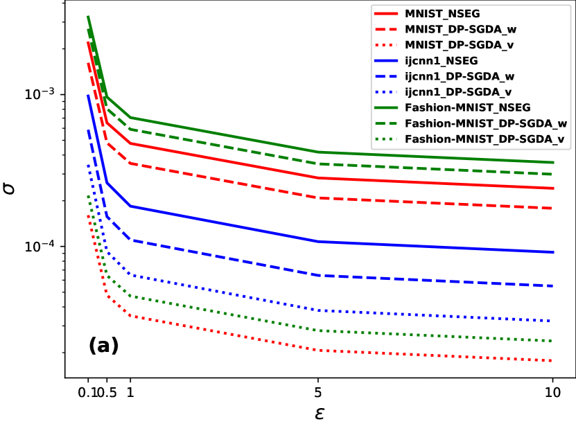
Figure 2: Comparison of $\sigma$ in NSEG and DP-SGDA (with Linear setting) on three datasets with different $\epsilon$ and (a) $\delta$=1e-5 and (b) $\delta$=1e-4.

References

• Abadi et al. [2016] Martin Abadi, Andy Chu, Ian Goodfellow, H Brendan McMahan, Ilya Mironov, Kunal Talwar, and Li Zhang. Deep learning with differential privacy. In Proceedings of the 2016 ACM SIGSAC conference on computer and communications security, pages 308–318, 2016.
• Abowd [2016] John M Abowd. The challenge of scientific reproducibility and privacy protection for statistical agencies. Census Scientific Advisory Committee, 2016.
• Arjovsky et al. [2017] Martin Arjovsky, Soumith Chintala, and Léon Bottou. Wasserstein generative adversarial networks. In ICML, pages 214–223. PMLR, 2017.
• Audibert and Catoni [2011] Jean-Yves Audibert and Olivier Catoni. Robust linear least squares regression. The Annals of Statistics, 39(5):2766–2794, 2011.
• Bassily et al. [2014] Raef Bassily, Adam Smith, and Abhradeep Thakurta. Private empirical risk minimization: Efficient algorithms and tight error bounds. In 2014 IEEE 55th Annual Symposium on Foundations of Computer Science, pages 464–473. IEEE, 2014.
• Bassily et al. [2019] Raef Bassily, Vitaly Feldman, Kunal Talwar, and Abhradeep Guha Thakurta. Private stochastic convex optimization with optimal rates. Advances in Neural Information Processing Systems, 32, 2019.
• Bassily et al. [2020] Raef Bassily, Vitaly Feldman, Cristóbal Guzmán, and Kunal Talwar. Stability of stochastic gradient descent on nonsmooth convex losses. Advances in Neural Information Processing Systems, 33:4381–4391, 2020.
• Beaulieu-Jones et al. [2019] Brett K Beaulieu-Jones, Zhiwei Steven Wu, Chris Williams, Ran Lee, Sanjeev P Bhavnani, James Brian Byrd, and Casey S Greene. Privacy-preserving generative deep neural networks support clinical data sharing. Circulation: Cardiovascular Quality and Outcomes, 12(7):e005122, 2019.
• Boob and Guzmán [2021] Digvijay Boob and Cristóbal Guzmán. Optimal algorithms for differentially private stochastic monotone variational inequalities and saddle-point problems. arXiv preprint arXiv:2104.02988, 2021.
• Bousquet and Elisseeff [2002] Olivier Bousquet and André Elisseeff. Stability and generalization. JMLR, 2(Mar):499–526, 2002.
• Chang and Lin [2011] Chih-Chung Chang and Chih-Jen Lin. Libsvm: a library for support vector machines. TIST, 2(3):27, 2011.
• Charles and Papailiopoulos [2018] Zachary Charles and Dimitris Papailiopoulos. Stability and generalization of learning algorithms that converge to global optima. In ICML, pages 745–754. PMLR, 2018.
• Diana et al. [2021] Emily Diana, Wesley Gill, Michael Kearns, Krishnaram Kenthapadi, and Aaron Roth. Minimax group fairness: Algorithms and experiments. In Proceedings of the 2021 AAAI/ACM Conference on AI, Ethics, and Society, pages 66–76, 2021.
• Ding et al. [2017] Bolin Ding, Janardhan Kulkarni, and Sergey Yekhanin. Collecting telemetry data privately. arXiv preprint arXiv:1712.01524, 2017.
• Dwork et al. [2006] Cynthia Dwork, Frank McSherry, Kobbi Nissim, and Adam Smith. Calibrating noise to sensitivity in private data analysis. In Theory of cryptography conference, pages 265–284. Springer, 2006.
• Dwork et al. [2014] Cynthia Dwork, Aaron Roth, et al. The algorithmic foundations of differential privacy. Foundations and Trends® in Theoretical Computer Science, 9(3–4):211–407, 2014.
• Erlingsson et al. [2014] Úlfar Erlingsson, Vasyl Pihur, and Aleksandra Korolova. Rappor: Randomized aggregatable privacy-preserving ordinal response. In ACM CCS, pages 1054–1067, 2014.
• Farnia and Ozdaglar [2021] Farzan Farnia and Asuman Ozdaglar. Train simultaneously, generalize better: Stability of gradient-based minimax learners. In ICML, pages 3174–3185. PMLR, 2021.
• Feldman et al. [2020] Vitaly Feldman, Tomer Koren, and Kunal Talwar. Private stochastic convex optimization: optimal rates in linear time. In Proceedings of the 52nd Annual ACM SIGACT Symposium on Theory of Computing, pages 439–449, 2020.
• Gao et al. [2013] Wei Gao, Rong Jin, Shenghuo Zhu, and Zhi-Hua Zhou. One-pass auc optimization. In ICML, pages 906–914. PMLR, 2013.
• Goodfellow et al. [2014] Ian Goodfellow, Jean Pouget-Abadie, Mehdi Mirza, Bing Xu, David Warde-Farley, Sherjil Ozair, Aaron Courville, and Yoshua Bengio. Generative adversarial nets. Advances in neural information processing systems, 27, 2014.
• Hardt et al. [2016] Moritz Hardt, Ben Recht, and Yoram Singer. Train faster, generalize better: Stability of stochastic gradient descent. In ICML, pages 1225–1234, 2016.
• Jordon et al. [2018] James Jordon, Jinsung Yoon, and Mihaela Van Der Schaar. Pate-gan: Generating synthetic data with differential privacy guarantees. In ICLR, 2018.
• Karimi et al. [2016] Hamed Karimi, Julie Nutini, and Mark Schmidt. Linear convergence of gradient and proximal-gradient methods under the polyak-łojasiewicz condition. In Joint European Conference on Machine Learning and Knowledge Discovery in Databases, pages 795–811. Springer, 2016.
• Kuzborskij and Lampert [2018] Ilja Kuzborskij and Christoph Lampert. Data-dependent stability of stochastic gradient descent. In ICML, pages 2815–2824. PMLR, 2018.
• LeCun et al. [1998] Yann LeCun, Léon Bottou, Yoshua Bengio, and Patrick Haffner. Gradient-based learning applied to document recognition. Proceedings of the IEEE, 86(11):2278–2324, 1998.
• Lei and Ying [2020] Yunwen Lei and Yiming Ying. Fine-grained analysis of stability and generalization for stochastic gradient descent. In ICML, pages 5809–5819. PMLR, 2020.
• Lei and Ying [2021] Yunwen Lei and Yiming Ying. Sharper generalization bounds for learning with gradient-dominated objective functions. In ICLR, 2021.
• Lei et al. [2021] Yunwen Lei, Zhenhuan Yang, Tianbao Yang, and Yiming Ying. Stability and generalization of stochastic gradient methods for minimax problems. In ICML, 2021.
• Li et al. [2019] Tian Li, Maziar Sanjabi, Ahmad Beirami, and Virginia Smith. Fair resource allocation in federated learning. arXiv preprint arXiv:1905.10497, 2019.
• Lin et al. [2020] Tianyi Lin, Chi Jin, and Michael Jordan. On gradient descent ascent for nonconvex-concave minimax problems. In ICML, pages 6083–6093. PMLR, 2020.
• Liu et al. [2020] Mingrui Liu, Zhuoning Yuan, Yiming Ying, and Tianbao Yang. Stochastic auc maximization with deep neural networks. In ICLR, 2020.
• Luo et al. [2020] Luo Luo, Haishan Ye, Zhichao Huang, and Tong Zhang. Stochastic recursive gradient descent ascent for stochastic nonconvex-strongly-concave minimax problems. Advances in Neural Information Processing Systems, 33:20566–20577, 2020.
• Martinez et al. [2020] Natalia Martinez, Martin Bertran, and Guillermo Sapiro. Minimax pareto fairness: A multi objective perspective. In International Conference on Machine Learning, pages 6755–6764. PMLR, 2020.
• Mohri et al. [2019] Mehryar Mohri, Gary Sivek, and Ananda Theertha Suresh. Agnostic federated learning. In International Conference on Machine Learning, pages 4615–4625. PMLR, 2019.
• Natole et al. [2018] M. Natole, Y. Ying, and S. Lyu. Stochastic proximal algorithms for auc maximization. In International Conference on Machine Learning, pages 3707–3716, 2018.
• Nedić and Ozdaglar [2009] Angelia Nedić and Asuman Ozdaglar. Subgradient methods for saddle-point problems. Journal of optimization theory and applications, 142(1):205–228, 2009.
• Nemirovski et al. [2009] Arkadi Nemirovski, Anatoli Juditsky, Guanghui Lan, and Alexander Shapiro. Robust stochastic approximation approach to stochastic programming. SIAM Journal on optimization, 19(4):1574–1609, 2009.
• Nouiehed et al. [2019] Maher Nouiehed, Maziar Sanjabi, Tianjian Huang, Jason D Lee, and Meisam Razaviyayn. Solving a class of non-convex min-max games using iterative first order methods. Advances in Neural Information Processing Systems, 32, 2019.
• Polyak [1964] Boris T Polyak. Gradient methods for solving equations and inequalities. USSR Computational Mathematics and Mathematical Physics, 4(6):17–32, 1964.
• Puterman [2014] Martin L Puterman. Markov decision processes: discrete stochastic dynamic programming. John Wiley & Sons, 2014.
• Rafique et al. [2021] Hassan Rafique, Mingrui Liu, Qihang Lin, and Tianbao Yang. Weakly-convex–concave min–max optimization: provable algorithms and applications in machine learning. Optimization Methods and Software, pages 1–35, 2021.
• Sinha et al. [2017] Aman Sinha, Hongseok Namkoong, Riccardo Volpi, and John Duchi. Certifying some distributional robustness with principled adversarial training. arXiv preprint arXiv:1710.10571, 2017.
• Song et al. [2013] Shuang Song, Kamalika Chaudhuri, and Anand D Sarwate. Stochastic gradient descent with differentially private updates. In 2013 IEEE Global Conference on Signal and Information Processing, pages 245–248. IEEE, 2013.
• Wang et al. [2019a] Di Wang, Changyou Chen, and Jinhui Xu. Differentially private empirical risk minimization with non-convex loss functions. In ICML, pages 6526–6535. PMLR, 2019a.
• Wang et al. [2020a] Di Wang, Hanshen Xiao, Srinivas Devadas, and Jinhui Xu. On differentially private stochastic convex optimization with heavy-tailed data. In International Conference on Machine Learning, pages 10081–10091. PMLR, 2020a.
• Wang [2017] Mengdi Wang. Primal-dual $\pi$ learning: Sample complexity and sublinear run time for ergodic markov decision problems. arXiv preprint arXiv:1710.06100, 2017.
• Wang et al. [2021a] Puyu Wang, Yunwen Lei, Yiming Ying, and Hai Zhang. Differentially private sgd with non-smooth loss. Applied and Computational Harmonic Analysis (ACHA), 2021a.
• Wang et al. [2021b] Puyu Wang, Zhenhuan Yang, Yunwen Lei, Yiming Ying, and Hai Zhang. Differentially private empirical risk minimization for auc maximization. Neurocomputing, 461:419–437, 2021b.
• Wang et al. [2020b] Serena Wang, Wenshuo Guo, Harikrishna Narasimhan, Andrew Cotter, Maya Gupta, and Michael Jordan. Robust optimization for fairness with noisy protected groups. Advances in Neural Information Processing Systems, 33:5190–5203, 2020b.
• Wang et al. [2019b] Yu-Xiang Wang, Borja Balle, and Shiva Prasad Kasiviswanathan. Subsampled rényi differential privacy and analytical moments accountant. In The 22nd International Conference on Artificial Intelligence and Statistics, pages 1226–1235. PMLR, 2019b.
• Wu et al. [2017] Xi Wu, Fengan Li, Arun Kumar, Kamalika Chaudhuri, Somesh Jha, and Jeffrey Naughton. Bolt-on differential privacy for scalable stochastic gradient descent-based analytics. In Proceedings of the 2017 ACM International Conference on Management of Data, pages 1307–1322, 2017.
• Xiao et al. [2017] Han Xiao, Kashif Rasul, and Roland Vollgraf. Fashion-mnist: a novel image dataset for benchmarking machine learning algorithms. arXiv preprint arXiv:1708.07747, 2017.
• Xie et al. [2018] Liyang Xie, Kaixiang Lin, Shu Wang, Fei Wang, and Jiayu Zhou. Differentially private generative adversarial network. arXiv preprint arXiv:1802.06739, 2018.
• Xu et al. [2009] Huan Xu, Constantine Caramanis, and Shie Mannor. Robustness and regularization of support vector machines. Journal of machine learning research, 10(7), 2009.
• Yan et al. [2020] Yan Yan, Yi Xu, Qihang Lin, Wei Liu, and Tianbao Yang. Optimal epoch stochastic gradient descent ascent methods for min-max optimization. Advances in Neural Information Processing Systems, 33:5789–5800, 2020.
• Ying et al. [2016] Yiming Ying, Longyin Wen, and Siwei Lyu. Stochastic online auc maximization. Advances in neural information processing systems, 29, 2016.
• Zhang et al. [2021a] Junyu Zhang, Mingyi Hong, Mengdi Wang, and Shuzhong Zhang. Generalization bounds for stochastic saddle point problems. In International Conference on Artificial Intelligence and Statistics, pages 568–576. PMLR, 2021a.
• Zhang et al. [2021b] Qiuchen Zhang, Jing Ma, Jian Lou, and Li Xiong. Private stochastic non-convex optimization with improved utility rates. In Proceedings of the Thirtieth International Joint Conference on Artificial Intelligence, IJCAI-21, pages 3370–3376, 2021b.
• Zhang et al. [2018] Xinyang Zhang, Shouling Ji, and Ting Wang. Differentially private releasing via deep generative model (technical report). arXiv preprint arXiv:1801.01594, 2018.
• Zhao et al. [2011] Peilin Zhao, Steven CH Hoi, Rong Jin, and Tianbao Yang. Online auc maximization. In ICML, 2011.
• Zhou et al. [2020] Yingxue Zhou, Xiangyi Chen, Mingyi Hong, Zhiwei Steven Wu, and Arindam Banerjee. Private stochastic non-convex optimization: Adaptive algorithms and tighter generalization bounds. arXiv preprint arXiv:2006.13501, 2020.