Parameter estimation for linear parabolic SPDEs in two space dimensions based on high frequency data

Abstract.

We consider parameter estimation for a linear parabolic second-order stochastic partial differential equation (SPDE) in two space dimensions driven by two types $Q$-Wiener processes based on high frequency data in time and space. We first estimate the parameters which appear in the coordinate process of the SPDE using the minimum contrast estimator based on the thinned data with respect to space, and then construct an approximate coordinate process of the SPDE. Furthermore, we propose estimators of the coefficient parameters of the SPDE utilizing the approximate coordinate process based on the thinned data with respect to time. We also give some simulation results.

1. Introduction

We consider the following linear parabolic stochastic partial differential equation (SPDE) in two space dimensions

$$\mathrm{d}X_{t}^{Q}(y,z) =\biggl{\{}\theta_{2}\biggl{(}\frac{\partial^{2}}{\partial y^{2}}+\frac{\partial^{2}}{\partial z^{2}}\biggr{)}+\theta_{1}\frac{\partial}{\partial y}+\eta_{1}\frac{\partial}{\partial z}+\theta_{0}\biggr{\}}X_{t}^{Q}(y,z)\mathrm{d}t$$

$$\qquad+\sigma\mathrm{d}W_{t}^{Q}(y,z),\quad(t,y,z)\in[0,1]\times D,$$ (1.1)

$$X_{0}^{Q}(y,z) =\xi(y,z),\quad(y,z)\in D,$$

$$X_{t}^{Q}(y,z) =0,\quad(t,y,z)\in[0,1]\times\partial D,$$

where $D=[0,1]^{2}$, $W_{t}^{Q}$ is a $Q$-Wiener process in a Sobolev space on $D$, an initial value $\xi$ is independent of $W_{t}^{Q}$, $\theta=(\theta_{0},\theta_{1},\eta_{1},\theta_{2})$ and $\sigma$ are unknown parameters and $(\theta_{0},\theta_{1},\eta_{1},\theta_{2},\sigma)\in\mathbb{R}^{3}\times(0,\infty)^{2}$. Moreover, the parameter space $\Theta$ is a compact convex subset of $\mathbb{R}^{3}\times(0,\infty)^{2}$, $\theta^{*}=(\theta_{0}^{*},\theta_{1}^{*},\eta_{1}^{*},\theta_{2}^{*})$ and $\sigma^{*}$ are true values of the parameters and we assume that $(\theta^{*},\sigma^{*})\in\mathrm{Int}\,\Theta$. The data are discrete observations $\{X_{t_{i}}^{Q}(y_{j_{1}},z_{j_{2}})\}$, $i=0,\ldots,N$, $j_{1}=0,\ldots,M_{1}$, $j_{2}=0,\ldots,M_{2}$ with $t_{i}=i\Delta_{N}$, $y_{j_{1}}=j_{1}/M_{1}$ and $z_{j_{2}}=j_{2}/M_{2}$, where $\Delta_{N}=1/N$ and $M:=M_{1}M_{2}$.

SPDEs appear in various fields such as physics, engineering, biology, and economics. In particular, the linear parabolic SPDE is a fundamental equation, and its typical example is the stochastic heat equation. The heat equation is known as the equation which describes the heat conduction in an object and the diffusion phenomenon of particles, and it is an essential equation which appears in various situations. For example, in the heat equation with one space dimension, we can consider the temperature variability of a thin object such as a wire, or a sea surface on a straight line. However, it is insufficient to consider practical problems with only a heat equation in one space dimension. Actually, in our daily problems, we often deal with two or three dimensional heat phenomena, such as temperature variability of a thin steel plate, sea surface, solid, or seawater. For instance, Piterbarg and Ostrovskii [20] treated sea surface temperature variability. Thus, it is important to analyze the SPDEs in two space dimensions because it can address more general problems than SPDEs in one space dimension.

Statistical inference for SPDE models based on discrete observations has been studied by many researchers, see, for example, Markussen [19], Bibinger and Trabs [1], Chong [3], [2], Cialenco et al. [5], Cialenco and Huang [7], Hildebrandt [9], Kaino and Uchida [13] and references therein. Recently, Kaino and Uchida [14] proposed the adaptive maximum likelihood type estimation for the coefficient parameters of linear parabolic second-order SPDEs in one space dimension with a small noise. Hildebrandt and Trabs [11], [10] studied the estimation for the coefficient parameters of linear parabolic and semilinear SPDEs in one space dimension, respectively, using a contrast function with double increments in time and space.

In particular, Bibinger and Trabs [1] treated the following linear parabolic SPDE in one space dimension

$$\mathrm{d}X_{t}(y) =\biggl{(}\theta_{2}\frac{\partial^{2}}{\partial y^{2}}+\theta_{1}\frac{\partial}{\partial y}+\theta_{0}\biggr{)}X_{t}(y)\mathrm{d}t+\sigma\mathrm{d}B_{t}(y),\quad(t,y)\in[0,T]\times[0,1],$$ (1.2)

$$X_{0}(y) =\xi(y),\quad y\in[0,1],\qquad X_{t}(0)=X_{t}(1)=0,\quad t\in[0,T],$$

where $T>0$, $B_{t}$ is a cylindrical Brownian motion in a Sobolev space on $[0,1]$, $\xi$ is an initial value, $\theta_{0},\theta_{1},\theta_{2}$ and $\sigma$ are unknown parameters and $(\theta_{0},\theta_{1},\theta_{2},\sigma)\in\mathbb{R}^{2}\times(0,\infty)^{2}$. They proposed minimum contrast estimators for $\kappa=\theta_{1}/\theta_{2}$, $\sigma_{0}^{2}=\sigma^{2}/\theta_{2}^{1/2}$ in the case where $T$ is fixed. Since the coordinate process $x_{k}(t)$, $k\geq 1$ of the SPDE (1.2) is expressed as

$$x_{k}(t)=\sqrt{2}\int_{0}^{1}X_{t}(y)\sin(\pi ky)\mathrm{e}^{\kappa y/2}\mathrm{d}y$$

and is a diffusion process satisfying the stochastic differential equation

$$\mathrm{d}x_{k}(t)=-\lambda_{k}x_{k}(t)\mathrm{d}t+\sigma\mathrm{d}w_{k}(t),\quad x_{k}(0)=\sqrt{2}\int_{0}^{1}\xi(y)\sin(\pi ky)\mathrm{e}^{\kappa y/2}\mathrm{d}y$$ (1.3)

where $\{w_{k}\}_{k\geq 1}$ is independent real valued standard Brownian motions and $\lambda_{k}=-\theta_{0}+\frac{\theta_{1}^{2}}{4\theta_{2}}+\pi^{2}k^{2}\theta_{2}$, Kaino and Uchida [13] constructed an approximate coordinate process by a Riemann sum

$$\hat{x}_{k}(t)=\frac{1}{M}\sum_{j=1}^{M}\sqrt{2}X_{t}(y_{j})\sin(\pi ky_{j})\mathrm{e}^{\hat{\kappa}y_{j}/2}$$

with observations of space $\{y_{j}\}_{j=1}^{M}$ and an estimator $\hat{\kappa}$ of $\kappa$, and proposed estimators of $\sigma^{2}$, $\theta_{2}$ and $\theta_{1}$ using the approximate coordinate process based on the thinned data with respect to time and statistical inference for diffusion processes. Furthermore, they extended the results of [1] to the case where $T$ is large and proposed estimators of $\sigma^{2}$, $\theta_{2}$, $\theta_{1}$ and $\theta_{0}$. For details of statistical inference for diffusion processes based on discrete observations, see Genon-Catalot and Jacod [8], Kessler [15], and Uchida and Yoshida [22], [23].

In this paper, we apply the estimation method based on the approximate coordinate process to SPDEs in two space dimensions and consider the estimation for each coefficient parameter of the SPDE (1.1). In this case, we need to be careful in setting a noise $W_{t}^{Q}$ because $X_{t}^{Q}$ may not be square integrable for any $t>0$ depending on the choice of the $Q$-Wiener process. Moreover, since the method of [13] is based on the property that the random filed $X_{t}$ admits a spectral decomposition

$$X_{t}(y)=\sum_{k=1}^{\infty}x_{k}(t)e_{k}(y)$$

with $e_{k}(y)=\sqrt{2}\sin(\pi ky)\mathrm{e}^{-\kappa y/2}$ and $x_{k}(t)$ in (1.3), it is also required to set a noise $W_{t}^{Q}$ such that the random field $X_{t}^{Q}$ in the SPDE (1.1) can be decomposed. See Hübner et al. [12] and Cialenco and Glatt-Holtz [6] for parameter estimation for SPDEs driven by a $Q$-Wiener process. See also the surveys by Lototsky [17] and Cialenco [4] for statistical inference based on the spectral approach.

This paper is organized as follows. In Section 2, we present the setting of our model. We also discuss how to choose a $Q$-Wiener process and introduce two types of $Q$-Wiener processes. In Section 3, we first propose minimum contrast estimators of the parameters appearing in the coordinate process of the SPDE by using the thinned data with respect to space. Next, we construct an approximate coordinate process by using these minimum contrast estimators, and provide estimators of the coefficient parameters of the SPDE based on the thinned data with respect to time. We then show that the estimators of the coefficient parameters are asymptotically normal. In Section 4, we give some simulation studies. Section 5 is devoted to the proofs of our assertions in Section 3. In order to understand the characteristics of the parameters of the SPDE (1.1), the sample paths with different values of the parameters are provided in Appendix section.

2. Preliminaries

Let $(\Omega,\mathscr{F},\{{\mathscr{F}}_{t}\}_{t\geq 0}P)$ be a stochastic basis with usual conditions, and let $\{w_{k,\ell}\}_{k,\ell\in\mathbb{N}}$ be independent real valued standard Brownian motions on this basis.

Let $A_{\theta}$ be the differential operator defined by

$$-A_{\theta}=\theta_{2}\biggl{(}\frac{\partial^{2}}{\partial y^{2}}+\frac{\partial^{2}}{\partial z^{2}}\biggr{)}+\theta_{1}\frac{\partial}{\partial y}+\eta_{1}\frac{\partial}{\partial z}+\theta_{0}.$$

Note that the SPDE (1.1) is represented as

$$\mathrm{d}X_{t}^{Q}(y,z)=-A_{\theta}X_{t}^{Q}(y,z)\mathrm{d}t+\sigma\mathrm{d}W_{t}^{Q}(y,z).$$

For $k,\ell\in\mathbb{N}$, the eigenfunctions $e_{k,\ell}$ of $A_{\theta}$ and the corresponding eigenvalues $\lambda_{k,\ell}$ are given by

$$e_{k,\ell}(y,z) =2\sin(\pi ky)\sin(\pi\ell z)\mathrm{e}^{-\frac{\theta_{1}}{2\theta_{2}}y}\mathrm{e}^{-\frac{\eta_{1}}{2\theta_{2}}z},\quad(y,z)\in D,$$

$$\lambda_{k,\ell} =-\theta_{0}+\frac{\theta_{1}^{2}+\eta_{1}^{2}}{4\theta_{2}}+\pi^{2}(k^{2}+\ell^{2})\theta_{2}.$$

We then obtain that $A_{\theta}e_{k,\ell}=\lambda_{k,\ell}e_{k,\ell}$ for $k,\ell\in\mathbb{N}$. For real valued functions $f$ and $g$ defined on $D$, let

$$\langle f,g\rangle_{\theta}=\int_{0}^{1}\int_{0}^{1}f(y,z)g(y,z)\mathrm{e}^{\frac{\theta_{1}}{\theta_{2}}y}\mathrm{e}^{\frac{\eta_{1}}{\theta_{2}}z}\mathrm{d}y\mathrm{d}z,\quad\|f\|_{\theta}=\langle f,f\rangle_{\theta}^{1/2}.$$

Moreover, set

$$H_{\theta}=\{f:D\to\mathbb{R}|\,\|f\|_{\theta}<\infty\text{ and }f(y,z)=0\text{ for }(y,z)\in\partial D\}.$$

We consider two types of $Q$-Wiener processes, $\{W_{t}^{Q_{1}}\}_{t\geq 0}$ and $\{W_{t}^{Q_{2}}\}_{t\geq 0}$, defined as follows.

$$\langle W_{t}^{Q_{1}},f\rangle_{\theta}=\sum_{k,\ell\geq 1}\lambda_{k,\ell}^{-\alpha/2}\langle f,e_{k,\ell}\rangle_{\theta}w_{k,\ell}(t),$$ (2.1)

$$\langle W_{t}^{Q_{2}},f\rangle_{\theta}=\sum_{k,\ell\geq 1}\mu_{k,\ell}^{-\alpha/2}\langle f,e_{k,\ell}\rangle_{\theta}w_{k,\ell}(t)$$ (2.2)

for $f\in H_{\theta}$ and $t\geq 0$, where $\mu_{k,\ell}=\pi^{2}(k^{2}+\ell^{2})+\mu_{0}$, $\mu_{0}\in(-2\pi^{2},\infty)$ and $\alpha\in(0,1)$. $\mu_{0}$ is an unknown parameter (may be known), the parameter space of $\mu_{0}$ is a compact convex subset of $(-2\pi^{2},\infty)$ and the true value $\mu_{0}^{*}$ belongs to its interior. The restriction $\alpha>0$ is for mathematical reasons, and the restriction $\alpha<1$ is for statistical inferences. See Remarks 1, 2 and 4 for details of the $Q$-Wiener processes and the restriction of $\alpha$.

We assume that $\xi\in H_{\theta}$ and $\lambda_{1,1}^{*}=-\theta_{0}^{*}+\frac{(\theta_{1}^{*})^{2}+(\eta_{1}^{*})^{2}}{4\theta_{2}^{*}}+2\pi^{2}\theta_{2}^{*}>0$. $X_{t}^{Q}$ is called a mild solution of (1.1) on $D$ if it satisfies that for any $t\in[0,1]$,

$$X_{t}^{Q}=\mathrm{e}^{-tA_{\theta}}\xi+\sigma\int_{0}^{t}\mathrm{e}^{-(t-s)A_{\theta}}\mathrm{d}W_{s}^{Q}\quad\mathrm{a.s.},$$

where $\mathrm{e}^{-tA_{\theta}}u=\sum_{k,\ell\geq 1}\mathrm{e}^{-\lambda_{k,\ell}t}\langle u,e_{k,\ell}\rangle_{\theta}e_{k,\ell}$ for $u\in H_{\theta}$. By defining the $Q_{1}$-Wiener process $W_{t}^{Q_{1}}$ in (2.1), the random field $X_{t}^{Q_{1}}(y,z)$ is expressed as

$$X_{t}^{Q_{1}}(y,z)=\sum_{k,\ell\geq 1}x_{k,\ell}^{Q_{1}}(t)e_{k,\ell}(y,z),$$ (2.3)

where the coordinate process

$$x_{k,\ell}^{Q_{1}}(t)=\langle X_{t}^{Q_{1}},e_{k,\ell}\rangle_{\theta}=\mathrm{e}^{-\lambda_{k,\ell}t}\langle\xi,e_{k,\ell}\rangle_{\theta}+\sigma\int_{0}^{t}\lambda_{k,\ell}^{-\alpha/2}\mathrm{e}^{-\lambda_{k,\ell}(t-s)}\mathrm{d}w_{k,\ell}(s)$$

is the Ornstein-Uhlenbeck process which satisfies the stochastic differential equation

$$\mathrm{d}x_{k,\ell}^{Q_{1}}(t)=-\lambda_{k,\ell}x_{k,\ell}^{Q_{1}}(t)\mathrm{d}t+\sigma\lambda_{k,\ell}^{-\alpha/2}\mathrm{d}w_{k,\ell}(t),\quad x_{k,\ell}^{Q_{1}}(0)=\langle\xi,e_{k,\ell}\rangle_{\theta}.$$

Note that

$$x_{k,\ell}^{Q_{1}}(t)=2\int_{0}^{1}\int_{0}^{1}X_{t}^{Q_{1}}(y,z)\sin(\pi ky)\sin(\pi\ell z)\mathrm{e}^{\frac{\theta_{1}}{2\theta_{2}}y}\mathrm{e}^{\frac{\eta_{1}}{2\theta_{2}}z}\mathrm{d}y\mathrm{d}z.$$ (2.4)

Similarly, by defining the $Q_{2}$-Wiener process $W_{t}^{Q_{2}}$ in (2.2), the random field $X_{t}^{Q_{2}}(y,z)$ is spectrally decomposed as

$$X_{t}^{Q_{2}}(y,z)=\sum_{k,\ell\geq 1}x_{k,\ell}^{Q_{2}}(t)e_{k,\ell}(y,z),$$

where the coordinate process

$$x_{k,\ell}^{Q_{2}}(t)=\langle X_{t}^{Q_{2}},e_{k,\ell}\rangle_{\theta}=\mathrm{e}^{-\lambda_{k,\ell}t}\langle\xi,e_{k,\ell}\rangle_{\theta}+\sigma\int_{0}^{t}\mu_{k,\ell}^{-\alpha/2}\mathrm{e}^{-\lambda_{k,\ell}(t-s)}\mathrm{d}w_{k,\ell}(s)$$

is described by the stochastic differential equation

$$\mathrm{d}x_{k,\ell}^{Q_{2}}(t)=-\lambda_{k,\ell}x_{k,\ell}^{Q_{2}}(t)\mathrm{d}t+\sigma\mu_{k,\ell}^{-\alpha/2}\mathrm{d}w_{k,\ell}(t),\quad x_{k,\ell}^{Q_{2}}(0)=\langle\xi,e_{k,\ell}\rangle_{\theta}$$ (2.5)

and is also represented as

$$x_{k,\ell}^{Q_{2}}(t)=2\int_{0}^{1}\int_{0}^{1}X_{t}^{Q_{2}}(y,z)\sin(\pi ky)\sin(\pi\ell z)\mathrm{e}^{\frac{\theta_{1}}{2\theta_{2}}y}\mathrm{e}^{\frac{\eta_{1}}{2\theta_{2}}z}\mathrm{d}y\mathrm{d}z.$$

Remark 1

Consider the case where the SPDE (1.1) is driven by a cylindrical Brownian motion $\{B_{t}\}_{t\geq 0}$ defined as

$$\langle B_{t},f\rangle_{\theta}=\sum_{k,\ell\geq 1}\langle f,e_{k,\ell}\rangle_{\theta}w_{k,\ell}(t),\quad f\in H_{\theta},\ t\geq 0$$ (2.6)

as in the setting of previous studies on parameter estimation for SPDEs in one space dimension, in other words, consider the SPDE represented by

$$\mathrm{d}X_{t}^{I}(y,z)=-A_{\theta}X_{t}^{I}(y,z)\mathrm{d}t+\sigma\mathrm{d}W_{t}^{I}(y,z),$$ (2.7)

where $I$ is the identity operator and $B_{t}=W_{t}^{I}$. In this case, the coordinate process $x_{k,\ell}^{I}(t)$ of the SPDE (2.7) is expressed as $x_{k,\ell}^{I}(t)=\mathrm{e}^{-\lambda_{k,\ell}t}\langle\xi,e_{k,\ell}\rangle_{\theta}$ $+\sigma\int_{0}^{t}\mathrm{e}^{-\lambda_{k,\ell}(t-s)}\mathrm{d}w_{k,\ell}(s)$. Since there exists a constant $C_{1}>0$ such that $\lambda_{k,\ell}\leq C_{1}(k^{2}+\ell^{2})$ for $k,\ell\geq 1$, it follows that for any $t>0$,

$$\mathbb{E}[\|X_{t}^{I}\|_{\theta}^{2}]=\sum_{k,\ell\geq 1}\mathbb{E}[x_{k,\ell}^{I}(t)^{2}] =\sum_{k,\ell\geq 1}\mathrm{e}^{-2\lambda_{k,\ell}t}\mathbb{E}[\langle\xi,e_{k,\ell}\rangle_{\theta}^{2}]+\sigma^{2}\sum_{k,\ell\geq 1}\frac{1-\mathrm{e}^{-2\lambda_{k,\ell}t}}{2\lambda_{k,\ell}}$$

$$\geq\sigma^{2}\sum_{k,\ell\geq 1}\frac{1-\mathrm{e}^{-2\lambda_{k,\ell}t}}{2\lambda_{k,\ell}}$$

$$\geq C\sum_{k,\ell\geq 1}\frac{1}{\lambda_{k,\ell}}=\infty,$$

and then $\mathbb{E}[X_{t}^{I}(y,z)^{2}]=\infty$ for some $(y,z)\in D$. In order to avoid this inconvenience, we consider a noise $W_{t}^{Q}$ with a damping factor such as $\{\lambda_{k,\ell}^{-\alpha/2}\}_{k,\ell\geq 1}$ in (2.1). Let $\mathscr{D}(A_{\theta}^{-1/2})\supset H_{\theta}$ be the domain of $A_{\theta}^{-1/2}$. Define the covariance operator $Q_{1}$ on $\mathscr{D}(A_{\theta}^{-1/2})$ by

$$Q_{1}e_{k,\ell}=\lambda_{k,\ell}^{-\alpha}\|e_{k,\ell}\|_{\theta,-1/2}^{2}e_{k,\ell},$$

where $\alpha>0$, $\|u\|_{\theta,-1/2}=\|A_{\theta}^{-1/2}u\|_{\theta}$, and then $\{e_{k,\ell}/\|e_{k,\ell}\|_{\theta,-1/2}\}_{k,\ell\geq 1}$ is the complete orthonormal system on $\mathscr{D}(A_{\theta}^{-1/2})$ and the corresponding eigenvalues of $Q_{1}$ are $\lambda_{k,\ell}^{-\alpha}\|e_{k,\ell}\|_{\theta,-1/2}^{2}$. Noting that

$$\sum_{k,\ell\geq 1}\|A_{\theta}^{-\alpha/2}e_{k,\ell}\|_{\theta,-1/2}^{2}=\sum_{k,\ell\geq 1}\frac{1}{\lambda_{k,\ell}^{1+\alpha}}<\infty$$

for $\alpha>0$, the $Q_{1}$-Wiener process $\{W_{t}^{Q_{1}}\}_{t\geq 0}$ is well-defined in $\mathscr{D}(A_{\theta}^{-1/2})$ and it follows that for $f\in H_{\theta}$,

$$\langle W^{Q_{1}}_{t},f\rangle_{\theta}=\sum_{k,\ell\geq 1}\lambda_{k,\ell}^{-\alpha/2}\|e_{k,\ell}\|_{\theta,-1/2}\biggl{\langle}f,\frac{e_{k,\ell}}{\|e_{k,\ell}\|_{\theta,-1/2}}\biggr{\rangle}_{\theta}w_{k,\ell}(t)=\sum_{k,\ell\geq 1}\lambda_{k,\ell}^{-\alpha/2}\langle f,e_{k,\ell}\rangle_{\theta}w_{k,\ell}(t),$$

and thus we obtain (2.1). Refer to Lord et al. [16], Da Prato and Zabczyk [21] and Lototsky and Rozovsky [18] for details on the $Q$-Wiener process.

Remark 2

Unlike the damping factor $\{\lambda_{k,\ell}^{-\alpha/2}\}_{k,\ell\geq 1}$ of the $Q_{1}$-Wiener process, the damping factor $\{\mu_{k,\ell}^{-\alpha/2}\}_{k,\ell\geq 1}$ of the $Q_{2}$-Wiener process does not include the parameter $\theta$ of the differential operator $A_{\theta}$. Moreover, by setting $\kappa=\theta_{1}/\theta_{2}$, $\eta=\eta_{1}/\theta_{2}$ and $\zeta=(\frac{\kappa^{2}+\eta^{2}}{4}-\mu_{0},\kappa,\eta,1)$, it can be regarded as

$$\mu_{k,\ell}=\pi^{2}(k^{2}+\ell^{2})+\mu_{0}=-\biggl{(}\frac{\kappa^{2}+\eta^{2}}{4}-\mu_{0}\biggr{)}+\frac{\kappa^{2}+\eta^{2}}{4\cdot 1}+\pi^{2}(k^{2}+\ell^{2})\cdot 1,$$

and it holds that $\langle\cdot,\cdot\rangle_{\zeta}=\langle\cdot,\cdot\rangle_{\theta}$, $H_{\zeta}=H_{\theta}$ and $A_{\zeta}e_{k,\ell}=\mu_{k,\ell}e_{k,\ell}$, where

$$-A_{\zeta}=\biggl{(}\frac{\partial^{2}}{\partial y^{2}}+\frac{\partial^{2}}{\partial z^{2}}\biggr{)}+\kappa\frac{\partial}{\partial y}+\eta\frac{\partial}{\partial z}+\biggl{(}\frac{\kappa^{2}+\eta^{2}}{4}-\mu_{0}\biggr{)}.$$

Hence, the $Q_{2}$-Wiener process can be constructed in the same way. Indeed, by choosing $Q_{2}$ as the covariance operator on $\mathscr{D}(A_{\zeta}^{-1/2})\supset H_{\zeta}(=H_{\theta})$ that satisfies

$$Q_{2}e_{k,\ell}=\mu_{k,\ell}^{-\alpha}\|e_{k,\ell}\|_{\zeta,-1/2}^{2}e_{k,\ell},$$

where $\alpha>0$, we can see that the $Q_{2}$-Wiener process $\{W_{t}^{Q_{2}}\}_{t\geq 0}$ is well-defined in $\mathscr{D}(A_{\zeta}^{-1/2})$ and

$$\langle W^{Q_{2}}_{t},f\rangle_{\theta}=\langle W^{Q_{2}}_{t},f\rangle_{\zeta}=\sum_{k,\ell\geq 1}\mu_{k,\ell}^{-\alpha/2}\langle f,e_{k,\ell}\rangle_{\zeta}w_{k,\ell}(t)=\sum_{k,\ell\geq 1}\mu_{k,\ell}^{-\alpha/2}\langle f,e_{k,\ell}\rangle_{\theta}w_{k,\ell}(t)$$

for $f\in H_{\theta}$ and $t\geq 0$.

In this paper, we consider only two types of $Q$-Wiener processes given by (2.1) or (2.2). However, the same argument can be developed by choosing a $Q$-Wiener process with a damping factor such that the random field $X_{t}^{Q}(y,z)$ is spectrally decomposable as in (2.3).

We assume the following conditions on the initial value $\xi\in H_{\theta}$ of the SPDE (1.1).

Assumption 1

The initial value $\xi$ satisfies either (i) or (ii), and both (iii) and (iv).

1. $\mathbb{E}[\langle\xi,e_{k,\ell}\rangle_{\theta}]=0$ for all $k,\ell\geq 1$ and $\sup_{k,\ell\geq 1}\lambda_{k,\ell}^{1+\alpha}\mathbb{E}[\langle\xi,e_{k}\rangle_{\theta}^{2}]<\infty$.

2. $\mathbb{E}[\|A_{\theta}^{(1+\alpha)/2}\xi\|_{\theta}^{2}]<\infty$.

3. $\sup_{k,\ell\geq 1}\lambda_{k,\ell}^{1+\alpha}\mathbb{E}[\langle\xi,e_{k,\ell}\rangle_{\theta}^{4}]<\infty$.

4. $\{\langle\xi,e_{k,\ell}\rangle_{\theta}\}_{k,\ell\geq 1}$ are independent.

Remark 3

From $\|A_{\theta}^{(1+\alpha)/2}\xi\|_{\theta}^{2}=\sum_{k,\ell\geq 1}\lambda_{k,\ell}^{1+\alpha}\langle\xi,e_{k,\ell}\rangle_{\theta}^{2}$, (ii) in Assumption 1 can be replaced by

$$\sum_{k,\ell\geq 1}\lambda_{k,\ell}^{1+\alpha}\mathbb{E}[\langle\xi,e_{k,\ell}\rangle_{\theta}^{2}]<\infty.$$

Moreover, for a non-random function $\xi(y,z)=\xi_{1}(y)\xi_{2}(z)\in H_{\theta}$, if $\xi_{1},\xi_{2}\in C^{2}([0,1])$ for $0<\alpha<1/2$, or if $\xi_{1},\xi_{2}\in C^{3}([0,1])$ for $1/2\leq\alpha<1$, then $\xi$ satisfies (ii) and (iii). Indeed, noting that

$$\langle\xi,e_{k,\ell}\rangle_{\theta}=2\int_{0}^{1}\xi_{1}(y)\sin(\pi ky)\mathrm{e}^{\frac{\theta_{1}}{2\theta_{2}}y}\mathrm{d}y\int_{0}^{1}\xi_{2}(z)\sin(\pi\ell z)\mathrm{e}^{\frac{\eta_{1}}{2\theta_{2}}z}\mathrm{d}z$$

and that for $\xi_{1}\in C^{p}([0,1])$ ($p=2,3$) such that $\xi_{1}(0)=\xi_{1}(1)=0$,

$$\Biggl{|}\int_{0}^{1}\xi_{1}(y)\sin(\pi ky)\mathrm{e}^{\frac{\theta_{1}}{2\theta_{2}}y}\mathrm{d}y\Biggr{|}\leq\frac{C_{1}}{k^{p}},$$

we obtain that $|\langle\xi,e_{k,\ell}\rangle_{\theta}|\leq C_{2}/k^{p}\ell^{p}$. Since $\lambda_{k,\ell}\leq C_{3}(k^{2}+\ell^{2})$ and

$$\sum_{k,\ell\geq 1}\lambda_{k,\ell}^{1+\alpha}\langle\xi,e_{k,\ell}\rangle_{\theta}^{2}\leq C\sum_{k,\ell\geq 1}\frac{(k^{2}+\ell^{2})^{1+\alpha}}{k^{2p}\ell^{2p}}\leq C^{\prime}\sum_{k\geq 1}\frac{1}{k^{2(p-1)-2\alpha}}\sum_{\ell\geq 1}\frac{1}{\ell^{2p}},$$

$\sum_{k,\ell\geq 1}\lambda_{k,\ell}^{1+\alpha}\langle\xi,e_{k,\ell}\rangle_{\theta}^{2}$ converges if $p>\alpha+3/2$, and therefore (ii) is satisfied by setting $p=2$ for $0<\alpha<1/2$ and $p=3$ for $1/2\leq\alpha<1$. Similarly, $\xi$ also satisfies (iii).

By setting the $Q_{1}$-Wiener process $W_{t}^{Q_{1}}$ by (2.1), there exists a unique mild solution $X_{t}^{Q_{1}}$ of the SPDE (1.1) which satisfies $\sup_{0\leq t\leq 1}\mathbb{E}[\|X_{t}^{Q_{1}}\|_{\theta}^{2}]<\infty$ under $\lambda_{1,1}^{*}>0$ and Assumption 1. Indeed, since $\sup_{k,\ell\geq 1}\lambda_{k,\ell}^{1+\alpha}\mathbb{E}[\langle\xi,e_{k}\rangle_{\theta}^{2}]<\infty$ under (i) or (ii) in Assumption 1 and that there exists a constant $C_{1}>0$ such that $\lambda_{k,\ell}\geq C_{1}(k^{2}+\ell^{2})$ for $k,\ell\geq 1$, it holds that

$$\mathbb{E}[\|X_{t}^{Q_{1}}\|_{\theta}^{2}]=\sum_{k,\ell\geq 1}\mathbb{E}[x_{k,\ell}^{Q_{1}}(t)^{2}] =\sum_{k,\ell\geq 1}\mathrm{e}^{-2\lambda_{k,\ell}t}\mathbb{E}[\langle\xi,e_{k,\ell}\rangle_{\theta}^{2}]+\sigma^{2}\sum_{k,\ell\geq 1}\frac{1-\mathrm{e}^{-2\lambda_{k,\ell}t}}{2\lambda_{k,\ell}^{1+\alpha}}$$

$$\leq\sum_{k,\ell\geq 1}\frac{1}{\lambda_{k,\ell}^{1+\alpha}}\lambda_{k,\ell}^{1+\alpha}\mathbb{E}[\langle\xi,e_{k,\ell}\rangle_{\theta}^{2}]+\sigma^{2}\sum_{k,\ell\geq 1}\frac{1}{2\lambda_{k,\ell}^{1+\alpha}}$$

$$\leq C\sum_{k,\ell\geq 1}\frac{1}{\lambda_{k,\ell}^{1+\alpha}}<\infty$$

for $\alpha>0$, and the mild solution $X_{t}^{Q_{1}}$ satisfies $\sup_{0\leq t\leq 1}\mathbb{E}[\|X_{t}^{Q_{1}}\|_{\theta}^{2}]<\infty$. The same is true for $X_{t}^{Q_{2}}$.

3. Main results

3.1. SPDE driven by $Q_{1}$-Wiener process

In this subsection, we deal with the SPDE (1.1) driven by the $Q_{1}$-Wiener process defined as (2.1). We first consider the estimation for the parameters which appear in the coordinate process (2.4) based on the thinned data with respect to space. Set $\overline{m}_{1}\leq M_{1}$ and $\overline{m}_{2}\leq M_{2}$ such that $\overline{m}:=\overline{m}_{1}\overline{m}_{2}=O(N^{\rho})$ for some $0<\rho<1\land 2(1-\alpha)$, and let

$$\overline{y}_{j_{1}} =\biggl{\lfloor}\frac{M_{1}}{\overline{m}_{1}}\biggr{\rfloor}\frac{j_{1}}{M_{1}},\quad j_{1}=0,\ldots,\overline{m}_{1},$$

$$\overline{z}_{j_{2}} =\biggl{\lfloor}\frac{M_{2}}{\overline{m}_{2}}\biggr{\rfloor}\frac{j_{2}}{M_{2}},\quad j_{2}=0,\ldots,\overline{m}_{2}.$$

For $\delta\in(0,1/2)$, there exist $J_{1},J_{2}\geq 1$, $m_{1},m_{2}\geq 1$ such that

$$\overline{y}_{J_{1}}<\delta\leq\overline{y}_{J_{1}+1}<\cdots<\overline{y}_{J_{1}+m_{1}}\leq 1-\delta<\overline{y}_{J_{1}+m_{1}+1},$$

$$\overline{z}_{J_{2}}<\delta\leq\overline{z}_{J_{2}+1}<\cdots<\overline{z}_{J_{2}+m_{2}}\leq 1-\delta<\overline{z}_{J_{2}+m_{2}+1},$$

and let

$$\widetilde{y}_{j_{1}} =\overline{y}_{J_{1}+j_{1}}=\biggl{\lfloor}\frac{M_{1}}{\overline{m}_{1}}\biggr{\rfloor}\frac{J_{1}+j_{1}}{M_{1}},\quad j_{1}=1,\ldots,m_{1},$$

$$\widetilde{z}_{j_{2}} =\overline{z}_{J_{2}+j_{2}}=\biggl{\lfloor}\frac{M_{2}}{\overline{m}_{2}}\biggr{\rfloor}\frac{J_{2}+j_{2}}{M_{2}},\quad j_{2}=1,\ldots,m_{2}$$

and $D_{\delta}=[\delta,1-\delta]^{2}\subset D$. Note that $m:=m_{1}m_{2}=O(N^{\rho})$ and $(\widetilde{y}_{j_{1}},\widetilde{z}_{j_{2}})\in D_{\delta}$ for any $j_{1}=1,\ldots,m_{1}$ and $j_{2}=1,\ldots,m_{2}$.

We write $\Delta_{i}X^{Q}(y,z)=X_{t_{i}}^{Q}(y,z)-X_{t_{i-1}}^{Q}(y,z)$. Let $\Gamma(s)=\int_{0}^{\infty}x^{s-1}\mathrm{e}^{-x}\mathrm{d}x$, $s>0$.

Proposition 3.1

Under Assumption 1, it holds that uniformly in $(y,z)\in D_{\delta}$,

$$\mathbb{E}[(\Delta_{i}X^{Q_{1}})^{2}(y,z)]=\Delta_{N}^{\alpha}\frac{\sigma^{2}\Gamma(1-\alpha)}{4\pi\alpha\theta_{2}}\mathrm{e}^{-\frac{\theta_{1}}{\theta_{2}}y}\mathrm{e}^{-\frac{\eta_{1}}{\theta_{2}}z}+r_{N,i}+O(\Delta_{N}),$$ (3.1)

where $\sum_{i=1}^{N}|r_{N,i}|=O(\Delta_{N}^{\alpha})$, and thus

$$\mathbb{E}\biggl{[}\frac{1}{N\Delta_{N}^{\alpha}}\sum_{i=1}^{N}(\Delta_{i}X^{Q_{1}})^{2}(y,z)\biggr{]}=\frac{\sigma^{2}\Gamma(1-\alpha)}{4\pi\alpha\theta_{2}}\mathrm{e}^{-\frac{\theta_{1}}{\theta_{2}}y}\mathrm{e}^{-\frac{\eta_{1}}{\theta_{2}}z}+O(\Delta_{N}^{1-\alpha}).$$

Remark 4

It follows from the proofs of Lemmas 5.3, 5.4 and Proposition 3.1 that

$$\mathbb{E}[(\Delta_{i}X^{Q_{1}})^{2}(y,z)]$$

$$=\sigma^{2}\sum_{k,\ell\geq 1}\frac{1-\mathrm{e}^{-\lambda_{k,\ell}\Delta_{N}}}{\lambda_{k,\ell}^{1+\alpha}}\biggl{(}1-\frac{1-\mathrm{e}^{-\lambda_{k,\ell}\Delta_{N}}}{2}\mathrm{e}^{-2\lambda_{k,\ell}(i-1)\Delta_{N}}\biggr{)}e_{k,\ell}^{2}(y,z)+r_{N,i},$$ (3.2)

where $r_{N,i}$ is the sequence in (3.1). According to Lemmas 5.2 and 5.4, the restriction of $\alpha$ allows us to approximate the summation in (3.2) containing $\lambda_{k,\ell}$ with unknown parameters by an explicit expression such as the main part in (3.1). This makes it possible to estimate $\sigma^{2}/\theta_{2}$, $\theta_{1}/\theta_{2}$ and $\eta_{1}/\theta_{2}$.

Let $s=\sigma^{2}/\theta_{2}$, $\kappa=\theta_{1}/\theta_{2}$, $\eta=\eta_{1}/\theta_{2}$ and

$$Z_{N}^{Q}(y,z)=\frac{1}{N\Delta_{N}^{\alpha}}\sum_{i=1}^{N}(\Delta_{i}X^{Q})^{2}(y,z).$$

By setting the contrast function

$$U_{N,m}^{(1)}(s,\kappa,\eta)=\sum_{j_{1}=1}^{m_{1}}\sum_{j_{2}=1}^{m_{2}}\biggl{(}Z_{N}^{Q_{1}}(\widetilde{y}_{j_{1}},\widetilde{z}_{j_{2}})-\frac{\Gamma(1-\alpha)}{4\pi\alpha}s\,\mathrm{e}^{-(\kappa\widetilde{y}_{j_{1}}+\eta\widetilde{z}_{j_{2}})}\biggr{)}^{2},$$

the minimum contrast estimators of $s$, $\kappa$ and $\eta$ are defined as

$$(\hat{s},\hat{\kappa},\hat{\eta})=\underset{(s,\kappa,\eta)\in\Xi_{1}}{\mathrm{arginf}}\,U_{N,m}^{(1)}(s,\kappa,\eta),$$

where $\Xi_{1}$ is a compact convex subset of $(0,\infty)\times\mathbb{R}^{2}$. We suppose that the true value $(s^{*},\kappa^{*},\eta^{*})$ belongs to $\mathrm{Int}\,\Xi_{1}$.

Theorem 3.2

Under Assumption 1, it holds that for any $\gamma<\frac{1}{2}\land(1-\alpha)-\frac{\rho}{2}$, as $N\to\infty$ and $m\to\infty$,

$$m^{1/2}N^{\gamma}\begin{pmatrix}\hat{s}-s^{*}\\ \hat{\kappa}-\kappa^{*}\\ \hat{\eta}-\eta^{*}\end{pmatrix}\stackrel{{\scriptstyle p}}{{\longrightarrow}}0.$$

Remark 5

Bibinger and Trabs [1], which dealt with the parameter estimation for linear parabolic SPDEs in one space dimension, showed that the estimators have asymptotic normality. On the other hand, in two space dimensions, the evaluation of the remainder in (3.1) is worse than that in one space dimension because of the increase in dimension, and the asymptotic normality can not be derived. However, it is possible to estimate each coefficient parameter even if the estimators do not have asymptotic normality. Theorem 3.2 shows that in two space dimensions, the estimators have $m^{1/2}N^{\gamma}$-consistency and $m^{1/2}N^{\gamma}=o(N^{\frac{1}{2}\land(1-\alpha)})$. In other words, the assertion in Theorem 3.2 can be regarded as

$$N^{\gamma^{\prime}}\begin{pmatrix}\hat{s}-s^{*}\\ \hat{\kappa}-\kappa^{*}\\ \hat{\eta}-\eta^{*}\end{pmatrix}\stackrel{{\scriptstyle p}}{{\longrightarrow}}0$$

for any $\gamma^{\prime}<\frac{1}{2}\land(1-\alpha)$.

Once we estimate $(s,\kappa,\eta)$, we can construct an approximation for the coordinate process

$$x_{k,\ell}^{Q_{1}}(t)=\langle X_{t}^{Q_{1}},e_{k,\ell}\rangle_{\theta}=2\int_{0}^{1}\int_{0}^{1}X_{t}^{Q_{1}}(y,z)\sin(\pi ky)\sin(\pi\ell z)\mathrm{e}^{\frac{\kappa}{2}y}\mathrm{e}^{\frac{\eta}{2}z}\mathrm{d}y\mathrm{d}z$$

by a Riemann sum. Furthermore, noting that the coordinate process $x_{k,\ell}^{Q_{1}}(t)$ satisfies

$$\mathrm{d}x_{k,\ell}^{Q_{1}}(t)=-\lambda_{k,\ell}x_{k,\ell}^{Q_{1}}(t)\mathrm{d}t+\sigma\lambda_{k,\ell}^{-\alpha/2}\mathrm{d}w_{k,\ell}(t),\quad x_{k,\ell}^{Q_{1}}(0)=\langle\xi,e_{k,\ell}\rangle_{\theta},$$

we can estimate the volatility parameter $\sigma_{k,\ell}:=\sigma\lambda_{k,\ell}^{-\alpha/2}$ by using statistical inference for diffusion processes. Since

$$\lambda_{1,2}=\biggl{(}\frac{\sigma_{1,1}^{2}}{\sigma_{1,2}^{2}}\biggr{)}^{1/\alpha}\lambda_{1,1},\quad\lambda_{1,1}=\biggl{(}\frac{\sigma^{2}}{\sigma_{1,1}^{2}}\biggr{)}^{1/\alpha}=\biggl{(}\frac{s\theta_{2}}{\sigma_{1,1}^{2}}\biggr{)}^{1/\alpha}$$

and $\lambda_{1,2}-\lambda_{1,1}=3\pi^{2}\theta_{2}$, $\theta_{2}$ can be expressed by using $s$, $\sigma_{1,1}$ and $\sigma_{1,2}$ as follows.

$$\theta_{2}=\Biggl{\{}\frac{3\pi^{2}}{s^{1/\alpha}}\Biggl{(}\frac{1}{\sigma_{1,2}^{2/\alpha}}-\frac{1}{\sigma_{1,1}^{2/\alpha}}\Biggr{)}^{-1}\Biggr{\}}^{\frac{\alpha}{1-\alpha}}.$$

$\sigma^{2}$, $\theta_{1}$, $\eta_{1}$ and $\theta_{0}$ can also be expressed by using $\theta_{2}$, $s$, $\kappa$, $\eta$ and $\lambda_{1,1}$ as follows.

$$\sigma^{2}=s\theta_{2},\quad\theta_{1}=\kappa\theta_{2},\quad\eta_{1}=\eta\theta_{2},$$

$$\theta_{0}=-\lambda_{1,1}+\biggl{(}\frac{\kappa^{2}+\eta^{2}}{4}+2\pi^{2}\biggr{)}\theta_{2}.$$

With the above in mind, we construct an approximate coordinate process by using the thinned data with respect to time, and consider the estimation for each coefficient parameter. Let $n\leq N$ and

$$\widetilde{t}_{i}=\biggl{\lfloor}\frac{N}{n}\biggr{\rfloor}\frac{i}{N},\quad i=0,\ldots,n.$$

As an approximation of $x_{k,\ell}^{Q_{1}}(t)$, we consider

$$\hat{x}_{k,\ell}^{Q_{1}}(\widetilde{t}_{i})=\frac{2}{M}\sum_{j_{1}=1}^{M_{1}}\sum_{j_{2}=1}^{M_{2}}X_{\widetilde{t}_{i}}^{Q_{1}}(y_{j_{1}},z_{j_{2}})\sin(\pi ky_{j_{1}})\sin(\pi\ell z_{j_{2}})\mathrm{e}^{\frac{\hat{\kappa}}{2}y_{j_{1}}}\mathrm{e}^{\frac{\hat{\eta}}{2}z_{j_{2}}},\quad i=1,\ldots,n.$$

By using the thinned data based on the approximate coordinate process $\{\hat{x}_{k,\ell}^{Q_{1}}(\widetilde{t}_{i})\}_{i=1}^{n}$, the estimator of $\sigma_{k,\ell}^{2}$ is defined as

$$\hat{\sigma}_{k,\ell}^{2}=\sum_{i=1}^{n}\bigl{(}\hat{x}_{k,\ell}^{Q_{1}}(\widetilde{t}_{i})-\hat{x}_{k,\ell}^{Q_{1}}(\widetilde{t}_{i-1})\bigr{)}^{2}.$$

Moreover, the estimators of $\theta_{2}$, $\sigma^{2}$, $\theta_{1}$, $\eta_{1}$ and $\theta_{0}$ are defined as

$$\hat{\theta}_{2} =\Biggl{\{}\frac{3\pi^{2}}{\hat{s}^{1/\alpha}}\Biggl{(}\frac{1}{(\hat{\sigma}_{1,2}^{2})^{1/\alpha}}-\frac{1}{(\hat{\sigma}_{1,1}^{2})^{1/\alpha}}\Biggr{)}^{-1}\Biggr{\}}^{\frac{\alpha}{1-\alpha}},$$

$$\hat{\sigma}^{2} =\hat{s}\hat{\theta}_{2},\quad\hat{\theta}_{1}=\hat{\kappa}\hat{\theta}_{2},\quad\hat{\eta}_{1}=\hat{\eta}\hat{\theta}_{2},$$

$$\hat{\theta}_{0} =-\hat{\lambda}_{1,1}+\biggl{(}\frac{\hat{\kappa}^{2}+\hat{\eta}^{2}}{4}+2\pi^{2}\biggr{)}\hat{\theta}_{2},\quad\hat{\lambda}_{1,1}=\biggl{(}\frac{\hat{s}\hat{\theta}_{2}}{\hat{\sigma}_{1,1}^{2}}\biggr{)}^{1/\alpha}.$$

Let $\boldsymbol{\vartheta}_{-1}^{*}=(\theta_{1}^{*},\eta_{1}^{*},\theta_{2}^{*},(\sigma^{*})^{2})^{\mathsf{T}}$,

$$c_{1} =(\lambda_{1,1}^{*})^{2}\biggl{(}\frac{\lambda_{1,2}^{*}}{\alpha}-\frac{\theta_{0}^{*}}{1-\alpha}\biggr{)}^{2}+(\lambda_{1,2}^{*})^{2}\biggl{(}\frac{\lambda_{1,1}^{*}}{\alpha}-\frac{\theta_{0}^{*}}{1-\alpha}\biggr{)}^{2},$$

$$c_{2} =\frac{-1}{1-\alpha}\biggl{\{}(\lambda_{1,1}^{*})^{2}\biggl{(}\frac{\lambda_{1,2}^{*}}{\alpha}-\frac{\theta_{0}^{*}}{1-\alpha}\biggr{)}+(\lambda_{1,2}^{*})^{2}\biggl{(}\frac{\lambda_{1,1}^{*}}{\alpha}-\frac{\theta_{0}^{*}}{1-\alpha}\biggr{)}\biggr{\}},$$

$$c_{3} =\frac{1}{(1-\alpha)^{2}}\bigl{\{}(\lambda_{1,1}^{*})^{2}+(\lambda_{1,2}^{*})^{2}\bigr{\}}$$

$$J =\frac{2}{9\pi^{4}(\theta_{2}^{*})^{2}}\begin{pmatrix}c_{1}&c_{2}(\boldsymbol{\vartheta}_{-1}^{*})^{\mathsf{T}}\\ c_{2}\boldsymbol{\vartheta}_{-1}^{*}&c_{3}\boldsymbol{\vartheta}_{-1}^{*}(\boldsymbol{\vartheta}_{-1}^{*})^{\mathsf{T}}\end{pmatrix},$$

where $\mathsf{T}$ denotes the transpose.

Theorem 3.3

Suppose Assumption 1 holds. Let $\gamma<\frac{1}{2}\land(1-\alpha)-\frac{\rho}{2}$.

1. Under $\frac{n^{1-\alpha}}{mN^{2\gamma}}\to 0$ and $\frac{n^{1-\alpha+\epsilon}}{M_{1}^{2\epsilon}\land M_{2}^{2\epsilon}}\to 0$ for some $\epsilon<\alpha$, it holds that as $n\to\infty$,

   $$(\hat{\theta}_{0},\hat{\theta}_{1},\hat{\eta}_{1},\hat{\theta}_{2},\hat{\sigma}^{2})\stackrel{{\scriptstyle p}}{{\longrightarrow}}(\theta_{0}^{*},\theta_{1}^{*},\eta_{1}^{*},\theta_{2}^{*},(\sigma^{*})^{2}).$$

2. Under $\frac{n^{2-\alpha}}{mN^{2\gamma}}\to 0$ and $\frac{n^{2-\alpha+\epsilon}}{M_{1}^{2\epsilon}\land M_{2}^{2\epsilon}}\to 0$ for some $\epsilon<\alpha$, it holds that as $n\to\infty$,

   $$\sqrt{n}\begin{pmatrix}\hat{\theta}_{0}-\theta_{0}^{*}\\ \hat{\theta}_{1}-\theta_{1}^{*}\\ \hat{\eta}_{1}-\eta_{1}^{*}\\ \hat{\theta}_{2}-\theta_{2}^{*}\\ \hat{\sigma}^{2}-(\sigma^{*})^{2}\end{pmatrix}\stackrel{{\scriptstyle d}}{{\longrightarrow}}N(0,J).$$

Remark 6

Set $M_{1}=M_{2}$, $M=O(N^{\beta})$, $\beta>0$, $n=O(N^{\zeta})$, $0<\zeta\leq 1$, and $m=O(N^{\rho})$, $0<\rho<1\land 2(1-\alpha)$. For the condition of (1) in Theorem 3.3, one has from $\frac{n^{1-\alpha}}{mN^{2\gamma}}=O(N^{\zeta(1-\alpha)-\rho-2\gamma})$, $\frac{n^{1-\alpha+\epsilon}}{M_{1}^{2\epsilon}\land M_{2}^{2\epsilon}}=O(N^{\zeta(1-\alpha+\epsilon)-\epsilon\beta})$ that

$$\zeta(1-\alpha)-\rho-2\gamma<0,\quad\zeta(1-\alpha+\epsilon)-\epsilon\beta<0$$ (3.3)

for some $\epsilon<\alpha$. For the existence of $\epsilon<\alpha$ such that $\zeta(1-\alpha+\epsilon)-\epsilon\beta<0$, it suffices that $\zeta(1-\alpha)/(\beta-\zeta)<\epsilon<\alpha$, i.e., $\zeta<\alpha\beta$. Therefore, (3.3) is fulfilled if $\zeta$ is chosen as follows.

$$\zeta<\frac{\rho+2\gamma}{1-\alpha}\land\alpha\beta.$$ (3.4)

Since we can choose $\gamma$ such that $1-\alpha<\rho+2\gamma$, (3.4) is represented by $\zeta<\alpha\beta$. In the same way as (2) in Theorem 3.3, we can choose $0<\zeta\leq 1$ such that

$$\zeta<\frac{\rho+2\gamma}{2-\alpha}\land\frac{\alpha\beta}{2},$$ (3.5)

and since $\gamma$ can be chosen to satisfy $\rho+2\gamma<1\land 2(1-\alpha)$, (3.5) is represented by $\zeta<\frac{1\land 2(1-\alpha)}{2-\alpha}\land\frac{\alpha\beta}{2}$. We also see from (3.4) and (3.5) that for some $\zeta<\frac{\rho+2\gamma}{2-\alpha}$, we need to set $\beta>\zeta/\alpha$ for consistency, and $\beta>2\zeta/\alpha$ for asymptotic normality. That is, in order to obtain asymptotic normality of the estimators, it is necessary to increase the number of observations in space $M$ compared to the number of observations in space required for consistency to hold.

3.2. SPDE driven by $Q_{2}$-Wiener process

In this subsection, we consider the SPDE (1.1) driven by the $Q_{2}$-Wiener process defined as (2.2). In this case, as in Subsection 3.1, we first estimate the parameters $\theta_{1}/\theta_{2}$ and $\eta_{1}/\theta_{2}$ which appear in the coordinate process, and then estimate the coefficient parameters using the approximate coordinate process.

In a similar way to Proposition 3.1, the following proposition holds.

Proposition 3.4

Under Assumption 1, it holds that uniformly in $(y,z)\in D_{\delta}$,

$$\mathbb{E}[(\Delta_{i}X^{Q_{2}})^{2}(y,z)]=\Delta_{N}^{\alpha}\frac{\sigma^{2}\Gamma(1-\alpha)}{4\pi\alpha\theta_{2}^{1-\alpha}}\mathrm{e}^{-\frac{\theta_{1}}{\theta_{2}}y}\mathrm{e}^{-\frac{\eta_{1}}{\theta_{2}}z}+r_{N,i}+O(\Delta_{N}),$$ (3.6)

where $\sum_{i=1}^{N}|r_{N,i}|=O(\Delta_{N}^{\alpha})$, and thus

$$\mathbb{E}\biggl{[}\frac{1}{N\Delta_{N}^{\alpha}}\sum_{i=1}^{N}(\Delta_{i}X^{Q_{2}})^{2}(y,z)\biggr{]} =\frac{\sigma^{2}\Gamma(1-\alpha)}{4\pi\alpha\theta_{2}^{1-\alpha}}\mathrm{e}^{-\frac{\theta_{1}}{\theta_{2}}y}\mathrm{e}^{-\frac{\eta_{1}}{\theta_{2}}z}+O(\Delta_{N}^{1-\alpha}).$$

Remark 7

The only difference between (3.1) and (3.6) is the exponent of $\theta_{2}$ in the denominator. This is caused by the fact that the coefficients of $k^{2}+\ell^{2}$ in $\lambda_{k,\ell}$ and $\mu_{k,\ell}$ are different, which are $\theta_{2}\pi^{2}$ and $\pi^{2}$ respectively. See Lemmas 5.1 and 5.5 for details. Proposition 3.4 allows us to estimate $\sigma^{2}/\theta_{2}^{1-\alpha}$, $\theta_{1}/\theta_{2}$ and $\eta_{1}/\theta_{2}$ when the SPDE (1.1) is driven by the $Q_{2}$-Wiener process.

Let $S=\sigma^{2}/\theta_{2}^{1-\alpha}$, $\kappa=\theta_{1}/\theta_{2}$, and $\eta=\eta_{1}/\theta_{2}$, and let

$$U_{N,m}^{(2)}(S,\kappa,\eta)=\sum_{j_{1}=1}^{m_{1}}\sum_{j_{2}=1}^{m_{2}}\biggl{(}Z_{N}^{Q_{2}}(\widetilde{y}_{j_{1}},\widetilde{z}_{j_{2}})-\frac{\Gamma(1-\alpha)}{4\pi\alpha}S\,\mathrm{e}^{-(\kappa\widetilde{y}_{j_{1}}+\eta\widetilde{z}_{j_{2}})}\biggr{)}^{2},$$

which is the contrast function of $S$, $\kappa$ and $\eta$. Let $\check{S}$, $\check{\kappa}$ and $\check{\eta}$ be minimum contrast estimators defined as

$$(\check{S},\check{\kappa},\check{\eta})=\underset{(S,\kappa,\eta)\in\Xi_{2}}{\mathrm{arginf}}\,U_{N,m}^{(2)}(S,\kappa,\eta),$$

where $\Xi_{2}$ is a compact convex subset of $(0,\infty)\times\mathbb{R}^{2}$, and we assume that the true value $(S^{*},\kappa^{*},\eta^{*})$ belongs to $\mathrm{Int}\,\Xi_{2}$.

Theorem 3.5

Under Assumption 1, it holds that for any $\gamma<\frac{1}{2}\land(1-\alpha)-\frac{\rho}{2}$, as $N\to\infty$ and $m\to\infty$,

$$m^{1/2}N^{\gamma}\begin{pmatrix}\check{S}-S^{*}\\ \check{\kappa}-\kappa^{*}\\ \check{\eta}-\eta^{*}\end{pmatrix}\stackrel{{\scriptstyle p}}{{\longrightarrow}}0.$$

We construct the following approximate coordinate process by using the estimators $\check{\kappa}$ and $\check{\eta}$.

$$\check{x}_{k,\ell}^{Q_{2}}(\widetilde{t}_{i})=\frac{2}{M}\sum_{j_{1}=1}^{M_{1}}\sum_{j_{2}=1}^{M_{2}}X_{\widetilde{t}_{i}}^{Q_{2}}(y_{j_{1}},z_{j_{2}})\sin(\pi ky_{j_{1}})\sin(\pi\ell z_{j_{2}})\mathrm{e}^{\frac{\hat{\kappa}}{2}y_{j_{1}}}\mathrm{e}^{\frac{\hat{\eta}}{2}z_{j_{2}}},\quad i=1,\ldots,n.$$

Noting that the coordinate process $x_{k,\ell}^{Q_{2}}(t)$ is a diffusion process given by (2.5), we can estimate the volatility parameter $\tau_{k,\ell}:=\sigma\mu_{k,\ell}^{-\alpha/2}$.

If $\mu_{0}$ is known, then the estimator of $\sigma^{2}$ is defined as

$$\check{\sigma}^{2}=\mu_{1,1}^{\alpha}\sum_{i=1}^{n}\bigl{(}\check{x}_{1,1}^{Q_{2}}(\widetilde{t}_{i})-\check{x}_{1,1}^{Q_{2}}(\widetilde{t}_{i-1})\bigr{)}^{2},$$

and the estimators of $\theta_{2}$, $\theta_{1}$ and $\eta_{1}$ are defined as

$$\check{\theta}_{2}=\biggl{(}\frac{\check{\sigma}^{2}}{\check{S}}\biggr{)}^{\frac{1}{1-\alpha}},\quad\check{\theta}_{1}=\check{\kappa}\check{\theta}_{2},\quad\check{\eta}_{1}=\check{\eta}\check{\theta}_{2}.$$

On the other hand, since

$$\mu_{1,1}=\biggl{(}\frac{\tau_{1,2}^{2}}{\tau_{1,1}^{2}}\biggr{)}^{1/\alpha}\mu_{1,2},\quad\mu_{1,2}=\mu_{1,1}+3\pi^{2},$$

$\mu_{1,1}$ and $\sigma^{2}$ can be expressed as

$$\mu_{1,1}=\frac{3\pi^{2}(\tau_{1,2}^{2}/\tau_{1,1}^{2})^{1/\alpha}}{1-(\tau_{1,2}^{2}/\tau_{1,1}^{2})^{1/\alpha}}=\frac{3\pi^{2}}{\tau_{1,1}^{2/\alpha}}\biggl{(}\frac{1}{\tau_{1,2}^{2/\alpha}}-\frac{1}{\tau_{1,1}^{2/\alpha}}\biggr{)}^{-1},$$

$$\sigma^{2}=\tau_{1,1}^{2}\mu_{1,1}^{\alpha}=\Biggl{\{}3\pi^{2}\biggl{(}\frac{1}{\tau_{1,2}^{2/\alpha}}-\frac{1}{\tau_{1,1}^{2/\alpha}}\biggr{)}^{-1}\Biggr{\}}^{\alpha}.$$

Therefore, if $\mu_{0}$ is unknown, then the estimators of $\tau_{k,\ell}^{2}$ and $\sigma^{2}$ are defined as

$$\bar{\tau}_{k,\ell}^{2}=\sum_{i=1}^{n}\bigl{(}\check{x}_{k,\ell}^{Q_{2}}(\widetilde{t}_{i})-\check{x}_{k,\ell}^{Q_{2}}(\widetilde{t}_{i-1})\bigr{)}^{2},$$

$$\bar{\sigma}^{2}=\Biggl{\{}3\pi^{2}\biggl{(}\frac{1}{(\bar{\tau}_{1,2}^{2})^{1/\alpha}}-\frac{1}{(\bar{\tau}_{1,1}^{2})^{1/\alpha}}\biggr{)}^{-1}\Biggr{\}}^{\alpha}$$

and the estimators of $\theta_{2}$, $\theta_{1}$, $\eta_{1}$ and $\mu_{0}$ are defined as

$$\bar{\theta}_{2}=\biggl{(}\frac{\bar{\sigma}^{2}}{\check{S}}\biggr{)}^{\frac{1}{1-\alpha}},\quad\bar{\theta}_{1}=\check{\kappa}\bar{\theta}_{2},\quad\bar{\eta}_{1}=\check{\eta}\bar{\theta}_{2},$$

$$\bar{\mu}_{0}=\bar{\mu}_{1,1}-2\pi^{2}=\frac{3\pi^{2}}{(\bar{\tau}_{1,1}^{2})^{1/\alpha}}\biggl{(}\frac{1}{(\bar{\tau}_{1,2}^{2})^{1/\alpha}}-\frac{1}{(\bar{\tau}_{1,1}^{2})^{1/\alpha}}\biggr{)}^{-1}-2\pi^{2}.$$

Let $\boldsymbol{\nu}_{-1}^{*}=(\theta_{1}^{*},\eta_{1}^{*},\theta_{2}^{*},(1-\alpha)(\sigma^{*})^{2})^{\mathsf{T}}$,

$$d_{1}=\frac{2(\mu_{1,1}^{*})^{2}(\mu_{1,2}^{*})^{2}}{\alpha^{2}},\quad d_{2}=\frac{\mu_{1,1}^{*}\mu_{1,2}^{*}(\mu_{1,1}^{*}+\mu_{1,2}^{*})}{\alpha(1-\alpha)},\quad d_{3}=\frac{(\mu_{1,1}^{*})^{2}+(\mu_{1,2}^{*})^{2}}{(1-\alpha)^{2}},$$

$$K=\frac{2}{(1-\alpha)^{2}}\boldsymbol{\nu}_{-1}^{*}(\boldsymbol{\nu}_{-1}^{*})^{\mathsf{T}},\quad L=\frac{2}{9\pi^{4}}\begin{pmatrix}d_{1}&d_{2}(\boldsymbol{\nu}_{-1}^{*})^{\mathsf{T}}\\ d_{2}\boldsymbol{\nu}_{-1}^{*}&d_{3}\boldsymbol{\nu}_{-1}^{*}(\boldsymbol{\nu}_{-1}^{*})^{\mathsf{T}}\end{pmatrix}.$$

Theorem 3.6

Suppose Assumption 1 holds. Let $\gamma<\frac{1}{2}\land(1-\alpha)-\frac{\rho}{2}$.

1. Let $\mu_{0}$ be known.

   1. Under $\frac{n^{1-\alpha}}{mN^{2\gamma}}\to 0$ and $\frac{n^{1-\alpha+\epsilon}}{M_{1}^{2\epsilon}\land M_{2}^{2\epsilon}}\to 0$ for some $\epsilon<\alpha$, it holds that as $n\to\infty$,

      $$(\check{\theta}_{1},\check{\eta}_{1},\check{\theta}_{2},\check{\sigma}^{2})\stackrel{{\scriptstyle p}}{{\longrightarrow}}(\theta_{1}^{*},\eta_{1}^{*},\theta_{2}^{*},(\sigma^{*})^{2}).$$

   2. Under $\frac{n^{2-\alpha}}{mN^{2\gamma}}\to 0$ and $\frac{n^{2-\alpha+\epsilon}}{M_{1}^{2\epsilon}\land M_{2}^{2\epsilon}}\to 0$ for some $\epsilon<\alpha$, it holds that as $n\to\infty$,

      $$\sqrt{n}\begin{pmatrix}\check{\theta}_{1}-\theta_{1}^{*}\\ \check{\eta}_{1}-\eta_{1}^{*}\\ \check{\theta}_{2}-\theta_{2}^{*}\\ \check{\sigma}^{2}-(\sigma^{*})^{2}\end{pmatrix}\stackrel{{\scriptstyle d}}{{\longrightarrow}}N(0,K).$$

2. Let $\mu_{0}$ be unknown.

   1. Under $\frac{n^{1-\alpha}}{mN^{2\gamma}}\to 0$ and $\frac{n^{1-\alpha+\epsilon}}{M_{1}^{2\epsilon}\land M_{2}^{2\epsilon}}\to 0$ for some $\epsilon<\alpha$, it holds that as $n\to\infty$,

      $$(\bar{\mu}_{0},\bar{\theta}_{1},\bar{\eta}_{1},\bar{\theta}_{2},\bar{\sigma}^{2})\stackrel{{\scriptstyle p}}{{\longrightarrow}}(\mu_{0}^{*},\theta_{1}^{*},\eta_{1}^{*},\theta_{2}^{*},(\sigma^{*})^{2}).$$

   2. Under $\frac{n^{2-\alpha}}{mN^{2\gamma}}\to 0$ and $\frac{n^{2-\alpha+\epsilon}}{M_{1}^{2\epsilon}\land M_{2}^{2\epsilon}}\to 0$ for some $\epsilon<\alpha$, it holds that as $n\to\infty$,

      $$\sqrt{n}\begin{pmatrix}\bar{\mu}_{0}-\mu_{0}^{*}\\ \bar{\theta}_{1}-\theta_{1}^{*}\\ \bar{\eta}_{1}-\eta_{1}^{*}\\ \bar{\theta}_{2}-\theta_{2}^{*}\\ \bar{\sigma}^{2}-(\sigma^{*})^{2}\end{pmatrix}\stackrel{{\scriptstyle d}}{{\longrightarrow}}N(0,L).$$

Remark 8

If $\mu_{0}$ is known, then the damping factor $\mu_{k,\ell}^{-\alpha/2}$ of the $Q_{2}$-Wiener process is known. Moreover, since the cylindrical Brownian motion is given by (2.6), the value corresponding to $\mu_{k,\ell}^{-\alpha/2}$ in (2.2) is $1$, that is, it is known. Therefore, it is natural to consider the $Q_{2}$-Wiener process when $\mu_{0}$ is known, since the $Q_{2}$-Wiener process can be regarded as the driving noise corresponding to a cylindrical Brownian motion in the sense that the value of the damping factor is known. Indeed, (a)-(2) in Theorem 3.6, especially for $\alpha=0.5$, corresponds to the result of Kaino and Uchida [13]. On the other hand, when $\mu_{0}$ is unknown, the $Q_{2}$-Wiener process corresponds to the $Q_{1}$-Wiener process in the sense that the damping factor is unknown. Theorem 3.3 and (b) in Theorem 3.6 show that $\theta_{0}$ can be estimated for the SPDE (1.1) driven by the $Q_{1}$-Wiener process, while $\mu_{0}$ can be estimated instead of $\theta_{0}$ for the SPDE (1.1) driven by the $Q_{2}$-Wiener process.

4. Simulations

The numerical solution of the SPDE (1.1) is generated by

$$\tilde{X}^{Q_{1}}_{t_{i}}(y_{j_{1}},z_{j_{2}})=\sum^{K}_{k=1}\sum^{L}_{\ell=1}x^{Q_{1}}_{k,\ell}(t_{i})e_{k,\ell}(y_{j_{1}},z_{j_{2}}),\quad i=1,...,N,j_{1}=1,...,M_{1},j_{2}=1,...,M_{2}.$$ (4.1)

For the characteristics of the parameters of the SPDE (1.1), see the Appendix below. In this simulation, the true values of parameters $(\theta_{0}^{*},\theta_{1}^{*},\eta_{1}^{*},\theta_{2}^{*},\sigma^{*})=(0,0.2,0.2,0.2,1)$. We set that $N=10^{3}$, $M_{1}=M_{2}=200$, $K=L=10^{5}$, $\xi=0$, $\alpha=0.5$, $\lambda_{1,1}^{*}\approx 4.05$. When $N=10^{3},M_{1}=M_{2}=200$, the size of data is about 10 GB. We used R language to compute the estimators of Theorems 3.2 and 3.3. The computation time of (4.1) is directly proportional to $K\times L$. Therefore, the computation time for the numerical solution of the SPDE (1.1) is directly proportional to $N\times M_{1}\times M_{2}\times K\times L$. In the setting of this simulation, $N\times M_{1}\times M_{2}\times K\times L=4\times 10^{17}$. Three personal computers were used for this simulation, and it takes about 100h to generate one sample path of the SPDE (1.1). The number of iteration is $25$ because the calculation time is enormous.

Figures 1-3 are sample paths of $X_{t}^{Q_{1}}(y,z)$ when $(\theta_{0}^{*},\theta_{1}^{*},\eta_{1}^{*},\theta_{2}^{*},\sigma^{*})=(0,0.2,0.2,0.2,1)$. Figure 1 is a cross section of the sample path at $t=0.1,0.5$ and $0.9$. Figure 2 is a cross section of the sample path at $y=0.1,0.5$ and $0.9$. From Figure 2, it can be seen that there is not much difference between the variation of the sample path near $z=0$ and that near $z=1$. Figure 3 is a cross section of the sample path at $z=0.1,0.5$ and $0.9$. From Figure 3, it can be seen that there is not much difference between the variation of the sample path near $y=0$ and that near $y=1$.

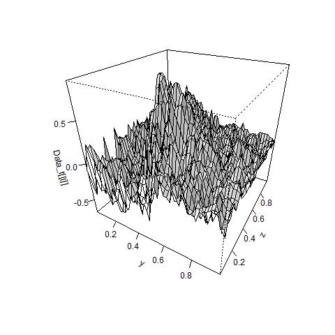
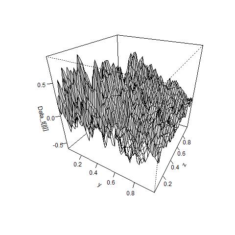
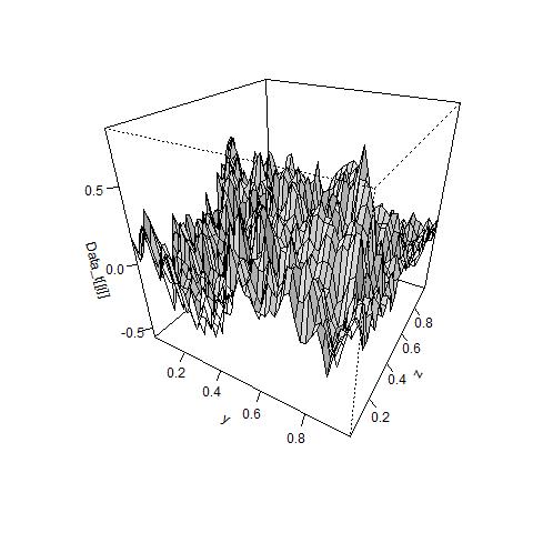
Figure 1. Cross sections of the sample path at $t=0.1$(left), $0.5$(center) and $0.9$(right)

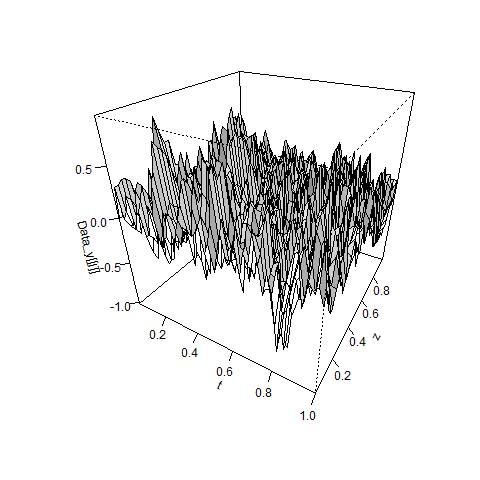
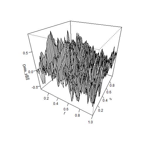
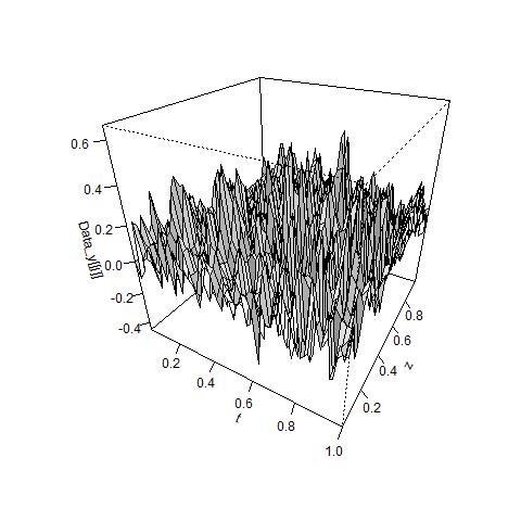
Figure 2. Cross sections of the sample path at $y=0.1$(left), $0.5$(center) and $0.9$(right)

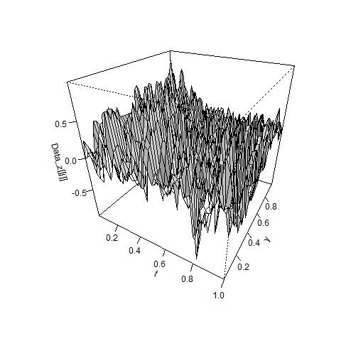
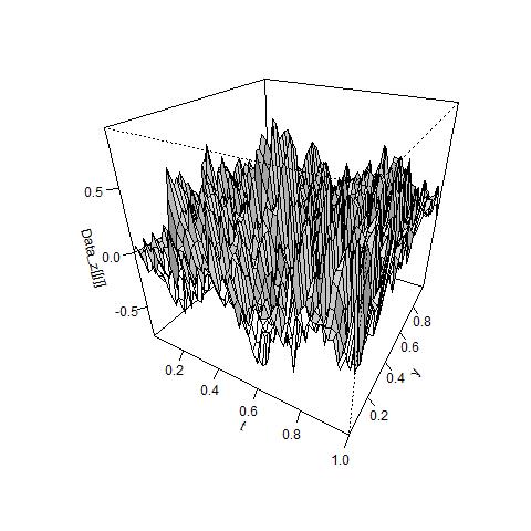
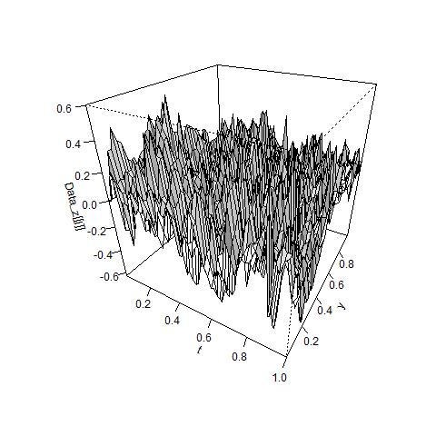
Figure 3. Cross sections of the sample path at $z=0.1$(left), $0.5$(center) and $0.9$(right)

First, we estimated $s=\sigma^{2}/\theta_{2}$, $\kappa=\theta_{1}/\theta_{2}$ and $\eta=\eta_{1}/\theta_{2}$. Table 1 is the simulation results of the means and the standard deviations (s.d.s) of $\hat{s}$, $\hat{\kappa}$ and $\hat{\eta}$ with $(N,m_{1},m_{2},\alpha,\rho,\gamma)=(10^{3},5,5,0.5,0.47,0.26)$.

Table 1. Simulation results of $\hat{s}$, $\hat{\kappa}$ and $\hat{\eta}$

	$\hat{s}$	$\hat{\kappa}$	$\hat{\eta}$
true value	5	1	1
mean	4.784	0.987	0.992
s.d.	(0.153)	(0.037)	(0.036)

It seems from Table 1 that the biases of $\hat{\kappa}$ and $\hat{\eta}$ are both very small and the result of $\hat{s}$ is not bad. The estimators of $s$, $\kappa$ and $\eta$ have good performances.

Next, we estimated $(\theta_{0},\theta_{1},\eta_{1},\theta_{2},\sigma^{2})$. Table 2 is the simulation results of the means and the standard deviations (s.d.s) of $\hat{\theta}_{0}$, $\hat{\theta}_{1}$, $\hat{\eta}_{1}$, $\hat{\theta}_{2}$ and $\hat{\sigma}^{2}$ with $(N,m_{1},m_{2},n,\alpha,\rho,\gamma,\epsilon)$ $=(10^{3},5,5,50,0.5,$ $0.47,0.26,0.499)$. In this case, $\frac{n^{1-\alpha}}{mN^{2\gamma}}\approx 0.008$ and $\frac{n^{1-\alpha+\epsilon}}{M_{1}^{2\epsilon}\land M_{2}^{2\epsilon}}\approx 0.25$.

Table 2. Simulation results of $\hat{\theta}_{0}$, $\hat{\theta}_{1}$, $\hat{\eta}_{1}$, $\hat{\theta}_{2}$ and $\hat{\sigma}^{2}$

	$\hat{\theta}_{0}$	$\hat{\theta}_{1}$	$\hat{\eta}_{1}$	$\hat{\theta}_{2}$	$\hat{\sigma}^{2}$
true value	0	0.2	0.2	0.2	1
mean	-0.291	0.150	0.152	0.152	0.732
s.d.	(2.710)	(0.081)	(0.085)	(0.083)	(0.403)

It seems from Table 2 that $\hat{\theta}_{0}$ has good performance. Although $\hat{\theta}_{1}$, $\hat{\eta}_{1}$, $\hat{\theta}_{2}$ and $\hat{\sigma}^{2}$ have small biases, their results are not bad.

Table 3 is the simulation results of the means and the standard deviations (s.d.s) of $\hat{\theta}_{0}$, $\hat{\theta}_{1}$, $\hat{\eta}_{1}$, $\hat{\theta}_{2}$ and $\hat{\sigma}^{2}$ with $(N,m_{1},m_{2},n,\alpha,\rho,\gamma,\epsilon)=(10^{3},5,5,100,0.5,0.47,0.26,0.499)$. In this case, $\frac{n^{1-\alpha}}{mN^{2\gamma}}\approx 0.011$ and $\frac{n^{1-\alpha+\epsilon}}{M_{1}^{2\epsilon}\land M_{2}^{2\epsilon}}\approx 0.50$.

Table 3. Simulation results of $\hat{\theta}_{0}$, $\hat{\theta}_{1}$, $\hat{\eta}_{1}$, $\hat{\theta}_{2}$ and $\hat{\sigma}^{2}$

	$\hat{\theta}_{0}$	$\hat{\theta}_{1}$	$\hat{\eta}_{1}$	$\hat{\theta}_{2}$	$\hat{\sigma}^{2}$
true value	0	0.2	0.2	0.2	1
mean	-0.862	0.190	0.191	0.191	0.904
s.d.	(3.393)	(0.080)	(0.081)	(0.081)	(0.416)

It seems from Table 3 that $\hat{\theta}_{1}$, $\hat{\eta}_{1}$, $\hat{\theta_{2}}$ and $\hat{\sigma}^{2}$ have good performances and that $\hat{\theta}_{0}$ has a small bias.

Table 4 is the simulation results of the means and the standard deviations (s.d.s) of $\hat{\theta}_{0}$, $\hat{\theta}_{1}$, $\hat{\eta}_{1}$, $\hat{\theta}_{2}$ and $\hat{\sigma}^{2}$ with $(N,m_{1},m_{2},n,\alpha,\rho,\gamma,\epsilon)=(10^{3},5,5,150,0.5,0.47,0.26,0.499)$. In this case, $\frac{n^{1-\alpha}}{mN^{2\gamma}}\approx 0.013$ and $\frac{n^{1-\alpha+\epsilon}}{M_{1}^{2\epsilon}\land M_{2}^{2\epsilon}}\approx 0.75$.

Table 4. Simulation results of $\hat{\theta}_{0}$, $\hat{\theta}_{1}$, $\hat{\eta}_{1}$, $\hat{\theta}_{2}$ and $\hat{\sigma}^{2}$

	$\hat{\theta}_{0}$	$\hat{\theta}_{1}$	$\hat{\eta}_{1}$	$\hat{\theta}_{2}$	$\hat{\sigma}^{2}$
true value	0	0.2	0.2	0.2	1
mean	-1.235	0.176	0.179	0.179	0.85
s.d.	(3.238)	(0.077)	(0.081)	(0.082)	(0.381)

It seems from Table 4 that $\hat{\theta}_{1}$, $\hat{\eta}_{1}$, $\hat{\theta_{2}}$ and $\hat{\sigma}^{2}$ have good performances and that $\hat{\theta}_{0}$ has a small bias.

At the moment, the number of iteration is only $25$, so the results are not very good. However, it is expected that the estimators have good performances if the number of iteration is increased.

5. Proofs

We set the following notation.

1. Let $\mathbb{R}_{+}=(0,\infty)$ and $\boldsymbol{k}=(k_{1},k_{2})\in\mathbb{N}^{2}$.

2. For $A,B\geq 0$, we write $A\lesssim B$ if $A\leq CB$ for some constant $C>0$.

3. For $x=(x_{1},\ldots,x_{d})\in\mathbb{R}^{d}$ and $f:\mathbb{R}^{d}\to\mathbb{R}$, we write $\partial_{x_{1}}f(x)=\frac{\partial}{\partial x_{1}}f(x)$, $\partial f(x)=(\partial_{x_{1}}f(x),\ldots,\partial_{x_{d}}f(x))$ and $\partial^{2}f(x)=(\partial_{x_{j}}\partial_{x_{i}}f(x))_{i,j=1}^{d}$.

4. For two functions $f$ and $g$, we write $f(s)\sim g(s)$ ($s\to s_{0}$) if there exists $c\in(0,\infty)$ such that $\lim_{s\to s_{0}}f(s)/g(s)=c$.

5. Let $\boldsymbol{1}_{A}$ be the indicator function of $A$.

6. Let $\mathrm{i}$ be the imaginary unit, and let $\mathrm{Re}(z)$ and $\mathrm{Im}(z)$ denote the real and imaginary parts of $z\in\mathbb{C}$, respectively.

5.1. Proofs of lemmas

In this subsection, we prepare some lemmas before proving our assertions in Section 3. For $\beta<2$, let $\mathcal{F}_{\beta}$ be the space of all twice continuously differentiable functions $f:\mathbb{R}_{+}\to\mathbb{R}$ satisfying the following conditions.

1. $sf(s^{2})$, $s^{2}f^{\prime}(s^{2})\boldsymbol{1}_{[1,\infty)}$, $s^{3}f^{\prime\prime}(s^{2})\boldsymbol{1}_{[1,\infty)}\in L^{1}(\mathbb{R}_{+})$.

2. $s^{\beta}f(s^{2})\sim 1$ ($s\downarrow 0$).

For $f\in\mathcal{F}_{\beta}$, we define

$$R_{1,N}=O\Biggl{(}\Delta_{N}\biggl{(}\int_{\Delta_{N}^{1/2}}^{1}s|f^{\prime}(s^{2})|\mathrm{d}s\lor\int_{\Delta_{N}^{1/2}}^{1}s^{3}|f^{\prime\prime}(s^{2})|\mathrm{d}s\biggr{)}\Biggr{)}$$

$$R_{2,N}=O\Biggl{(}\Delta_{N}^{3/2}\int_{\Delta_{N}^{1/2}}^{1}|f^{\prime}(s^{2})|\mathrm{d}s\Biggr{)},\quad R_{N}^{(\beta)}=O\Biggl{(}\Delta_{N}^{1/2}\int_{\Delta_{N}^{1/2}}^{1}s^{-\beta}\mathrm{d}s\Biggr{)}.$$

Let

$$D_{N}^{(1)} =\biggl{\{}(x_{1},x_{2})\in\mathbb{R}^{2}\biggl{|}0<x_{1}\leq\frac{\Delta_{N}^{1/2}}{2},\ \frac{\Delta_{N}^{1/2}}{2}<x_{2}\biggl{\}},$$

$$D_{N}^{(2)} =\biggl{\{}(x_{1},x_{2})\in\mathbb{R}^{2}\biggl{|}\frac{\Delta_{N}^{1/2}}{2}<x_{1},\ 0<x_{2}\leq\frac{\Delta_{N}^{1/2}}{2}\biggl{\}}.$$

Lemma 5.1

If $f\in\mathcal{F}_{\beta}$, then the followings hold.

1. $\displaystyle\Delta_{N}\sum_{\boldsymbol{k}\in\mathbb{N}^{2}}f(\lambda_{\boldsymbol{k}}\Delta_{N})=\frac{1}{4\pi\theta_{2}}\int_{0}^{\infty}f(s)\mathrm{d}s-\int_{D_{N}^{(1)}\cup D_{N}^{(2)}}f(\theta_{2}\pi^{2}|x|^{2})\mathrm{d}x+O(R_{1,N}\lor\Delta_{N}^{1-\beta/2})$.

2. For any $y,z\in[\delta,1-\delta]$,

   $$\Delta_{N}\sum_{\boldsymbol{k}\in\mathbb{N}^{2}}f(\lambda_{\boldsymbol{k}}\Delta_{N})\cos(2\pi k_{1}y) =-\int_{D_{N}^{(1)}}f(\theta_{2}\pi^{2}|x|^{2})\mathrm{d}x+O\biggl{(}\frac{R_{1,N}\lor R_{2,N}}{\delta^{2}}\biggr{)},$$

   $$\Delta_{N}\sum_{\boldsymbol{k}\in\mathbb{N}^{2}}f(\lambda_{\boldsymbol{k}}\Delta_{N})\cos(2\pi k_{2}z) =-\int_{D_{N}^{(2)}}f(\theta_{2}\pi^{2}|x|^{2})\mathrm{d}x+O\biggl{(}\frac{R_{1,N}\lor R_{2,N}}{\delta^{2}}\biggr{)}.$$

3. For any $y,z\in[\delta,1-\delta]$,

   $$\Delta_{N}\sum_{\boldsymbol{k}\in\mathbb{N}^{2}}f(\lambda_{\boldsymbol{k}}\Delta_{N})\cos(2\pi k_{1}y)\cos(2\pi k_{2}z)=O\biggl{(}\frac{R_{1,N}\lor R_{2,N}\lor\Delta_{N}^{1-\beta/2}}{\delta^{3}}\biggr{)}.$$

Furthermore, it holds that

$$\int_{D_{N}^{(1)}\cup D_{N}^{(2)}}f(\theta_{2}\pi^{2}|x|^{2})\mathrm{d}x=O(R_{N}^{(\beta)}).$$ (5.1)

Proof.

Let $K_{N}=\{x\in\mathbb{R}_{+}^{2}|c_{1}\Delta_{N}^{1/2}<|x|\}$ for $c_{1}>0$. Let $\varphi:\mathbb{R}_{+}\to\mathbb{R}$ be a function satisfying (a), and let $h(x)=\varphi(c_{2}|x|^{2})$, $c_{2}>0$. Since

$$\int_{\{x\in\mathbb{R}_{+}^{2}|c_{1}\Delta_{N}^{1/2}<|x|\leq 1\}}|\varphi^{\prime}(c_{2}|x|^{2})|\mathrm{d}x =\int_{0}^{\pi/2}\mathrm{d}\theta\int_{c_{1}\Delta_{N}^{1/2}}^{1}s|\varphi^{\prime}(c_{2}s^{2})|\mathrm{d}s=O\biggl{(}\int_{\Delta_{N}^{1/2}}^{1}s|\varphi^{\prime}(s^{2})|\mathrm{d}s\biggr{)},$$

$$\int_{\{x\in\mathbb{R}_{+}^{2}|1<|x|\}}|\varphi^{\prime}(c_{2}|x|^{2})|\mathrm{d}x =\int_{0}^{\pi/2}\mathrm{d}\theta\int_{1}^{\infty}s|\varphi^{\prime}(c_{2}s^{2})|\mathrm{d}s=O(1),$$

we have

$$\int_{K_{N}}|\varphi^{\prime}(c_{2}|x|^{2})|\mathrm{d}x =O\biggl{(}\int_{\Delta_{N}^{1/2}}^{1}s|\varphi^{\prime}(s^{2})|\mathrm{d}s\lor 1\biggr{)}=O\biggl{(}\int_{\Delta_{N}^{1/2}}^{1}s|\varphi^{\prime}(s^{2})|\mathrm{d}s\biggr{)}.$$ (5.2)

Similarly, we obtain

$$\int_{K_{N}}|x|^{2}|\varphi^{\prime\prime}(c_{2}|x|^{2})|\mathrm{d}x=O\biggl{(}\int_{\Delta_{N}^{1/2}}^{1}s^{3}|\varphi^{\prime\prime}(s^{2})|\mathrm{d}s\biggr{)}.$$ (5.3)

Therefore, it follows from (5.2), (5.3) and

$$\partial^{2}h(x) =4c_{2}^{2}\varphi^{\prime\prime}(c_{2}|x|^{2})\begin{pmatrix}x_{1}^{2}&x_{1}x_{2}\\ x_{1}x_{2}&x_{2}^{2}\end{pmatrix}+2c_{2}\varphi^{\prime}(c_{2}|x|^{2})\begin{pmatrix}1&0\\ 0&1\end{pmatrix}$$

that

$$\Delta_{N}\int_{K_{N}}|\partial^{2}h(x)|\mathrm{d}x =O\Biggl{(}\Delta_{N}\biggl{(}\int_{K_{N}}|x|^{2}|\varphi^{\prime\prime}(c_{2}|x|^{2})|\mathrm{d}x+\int_{K_{N}}|\varphi^{\prime}(c_{2}|x|^{2})|\mathrm{d}x\biggr{)}\Biggr{)}=O(R_{1,N}).$$ (5.4)

(1) Let $g(x)=f(\theta_{2}\pi^{2}|x|^{2})$, $a_{N}^{(k)}=(k+1/2)\Delta_{N}^{1/2}$ for $k\geq 0$,

$$E_{N}^{(\boldsymbol{k})} =(a_{N}^{(k_{1}-1)},a_{N}^{(k_{1})}]\times(a_{N}^{(k_{2}-1)},a_{N}^{(k_{2})}]\subset\mathbb{R}_{+}^{2},$$

$E_{N}=\bigcup_{\boldsymbol{k}\in\mathbb{N}^{2}}E_{N}^{(\boldsymbol{k})}$ and $F_{N}=\{x\in\mathbb{R}_{+}^{2}|(2\theta_{2}\pi^{2}\land\lambda_{1,1})^{1/2}\Delta_{N}^{1/2}<|x|\}$. By the Taylor expansion and (5.4), it follows that

$$\Biggl{|}\Delta_{N}\sum_{\boldsymbol{k}\in\mathbb{N}^{2}}f(\lambda_{\boldsymbol{k}}\Delta_{N})-\sum_{\boldsymbol{k}\in\mathbb{N}^{2}}\int_{E_{N}^{(\boldsymbol{k})}}f(\theta_{2}\pi^{2}|\boldsymbol{k}|^{2}\Delta_{N})\mathrm{d}x\Biggr{|}$$

$$=\Biggl{|}\Delta_{N}\sum_{\boldsymbol{k}\in\mathbb{N}^{2}}\biggl{(}f(\theta_{2}\pi^{2}|\boldsymbol{k}|^{2}\Delta_{N})$$

$$\qquad\qquad+\int_{0}^{1}f^{\prime}(\theta_{2}\pi^{2}|\boldsymbol{k}|^{2}\Delta_{N}+u(\lambda_{\boldsymbol{k}}-\theta_{2}\pi^{2}|\boldsymbol{k}|^{2})\Delta_{N})\mathrm{d}u\Bigl{(}\frac{\theta_{1}^{2}+\eta_{1}^{2}}{4\theta_{2}}-\theta_{0}\Bigr{)}\Delta_{N}\biggr{)}$$

$$\qquad\qquad-\sum_{\boldsymbol{k}\in\mathbb{N}^{2}}\int_{E_{N}^{(\boldsymbol{k})}}f(\theta_{2}\pi^{2}|\boldsymbol{k}|^{2}\Delta_{N})\mathrm{d}x\Biggr{|}$$

$$\leq\Delta_{N}\sum_{\boldsymbol{k}\in\mathbb{N}^{2}}\int_{0}^{1}\bigl{|}f^{\prime}(\theta_{2}\pi^{2}|\boldsymbol{k}|^{2}\Delta_{N}+u(\lambda_{\boldsymbol{k}}-\theta_{2}\pi^{2}|\boldsymbol{k}|^{2})\Delta_{N})\bigr{|}\mathrm{d}u\Bigl{|}\frac{\theta_{1}^{2}+\eta_{1}^{2}}{4\theta_{2}}-\theta_{0}\Bigr{|}\Delta_{N}$$

$$=O\biggl{(}\Delta_{N}\int_{F_{N}}|f^{\prime}(|x|^{2})|\mathrm{d}x\biggr{)}=O(R_{1,N})$$ (5.5)

and that

$$\Biggl{|}\sum_{\boldsymbol{k}\in\mathbb{N}^{2}}\int_{E_{N}^{(\boldsymbol{k})}}f(\theta_{2}\pi^{2}|\boldsymbol{k}|^{2}\Delta_{N})\mathrm{d}x-\int_{E_{N}}f(\theta_{2}\pi^{2}|x|^{2})\mathrm{d}x\Biggr{|}$$

$$=\Biggl{|}\sum_{\boldsymbol{k}\in\mathbb{N}^{2}}\int_{E_{N}^{(\boldsymbol{k})}}\bigl{(}g(\boldsymbol{k}\Delta_{N}^{1/2})-g(x)\bigr{)}\mathrm{d}x\Biggr{|}$$

$$=\Biggl{|}\sum_{\boldsymbol{k}\in\mathbb{N}^{2}}\int_{E_{N}^{(\boldsymbol{k})}}\biggl{(}\partial g(\boldsymbol{k}\Delta_{N}^{1/2})(x-\boldsymbol{k}\Delta_{N}^{1/2})$$

$$\qquad\qquad+\frac{1}{2}(x-\boldsymbol{k}\Delta_{N}^{1/2})^{\mathsf{T}}\int_{0}^{1}\partial^{2}g(\boldsymbol{k}\Delta_{N}^{1/2}+u(x-\boldsymbol{k}\Delta_{N}^{1/2}))\mathrm{d}u(x-\boldsymbol{k}\Delta_{N}^{1/2})\biggr{)}\mathrm{d}x\Biggr{|}$$

$$=\frac{1}{2}\Biggl{|}\sum_{\boldsymbol{k}\in\mathbb{N}^{2}}\int_{E_{N}^{(\boldsymbol{k})}}(x-\boldsymbol{k}\Delta_{N}^{1/2})^{\mathsf{T}}\int_{0}^{1}\partial^{2}g(\boldsymbol{k}\Delta_{N}^{1/2}+u(x-\boldsymbol{k}\Delta_{N}^{1/2}))\mathrm{d}u(x-\boldsymbol{k}\Delta_{N}^{1/2})\mathrm{d}x\Biggr{|}$$

$$\leq\frac{1}{2}\sum_{\boldsymbol{k}\in\mathbb{N}^{2}}\int_{E_{N}^{(\boldsymbol{k})}}\int_{0}^{1}\bigl{|}\partial^{2}g(\boldsymbol{k}\Delta_{N}^{1/2}+u(x-\boldsymbol{k}\Delta_{N}^{1/2}))\bigr{|}\mathrm{d}u|x-\boldsymbol{k}\Delta_{N}^{1/2}|^{2}\mathrm{d}x$$

$$\lesssim\Delta_{N}\sum_{\boldsymbol{k}\in\mathbb{N}^{2}}\int_{E_{N}^{(\boldsymbol{k})}}|\partial^{2}g(x)|\mathrm{d}x$$

$$=O\biggl{(}\Delta_{N}\int_{E_{N}}|\partial^{2}g(x)|\mathrm{d}x\biggr{)}=O(R_{1,N}).$$ (5.6)

Therefore, it follows from (5.5) and (5.6) that

$$\Delta_{N}\sum_{\boldsymbol{k}\in\mathbb{N}^{2}}f(\lambda_{\boldsymbol{k}}\Delta_{N}) =\int_{E_{N}}f(\theta_{2}\pi^{2}|x|^{2})\mathrm{d}x+O(R_{1,N}).$$ (5.7)

Set $D_{N}^{(3)}=\{(x_{1},x_{2})\in\mathbb{R}^{2}|0<x_{1},x_{2}\leq\Delta_{N}^{1/2}/2\}$ and $D_{N}=\bigcup_{j=1,2,3}D_{N}^{(j)}$. Since $sf(s^{2})\in L^{1}(\mathbb{R}_{+})$, $\int_{\mathbb{R}_{+}^{2}}|f(\theta_{2}\pi^{2}|x|^{2})|\mathrm{d}x<\infty$ and

$$\int_{\mathbb{R}_{+}^{2}}f(\theta_{2}\pi^{2}|x|^{2})\mathrm{d}x=\frac{1}{\pi^{2}\theta_{2}}\int_{0}^{\pi/2}\mathrm{d}\theta\int_{0}^{\infty}sf(s^{2})\mathrm{d}s=\frac{1}{4\pi\theta_{2}}\int_{0}^{\infty}f(s)\mathrm{d}s,$$

(5.7) can be expressed from $E_{N}=\mathbb{R}_{+}^{2}\setminus D_{N}$ as

$$\Delta_{N}\sum_{\boldsymbol{k}\in\mathbb{N}^{2}}f(\lambda_{\boldsymbol{k}}\Delta_{N})=\frac{1}{4\pi\theta_{2}}\int_{0}^{\infty}f(s)\mathrm{d}s-\int_{D_{N}}f(\theta_{2}\pi^{2}|x|^{2})\mathrm{d}x+O(R_{1,N}).$$ (5.8)

Let $a_{N}=\Delta_{N}^{1/2}/\sqrt{2}$. From $s^{\beta}f(s^{2})\sim 1$ $(s\downarrow 0)$, we see that $s|f(s^{2})|\lesssim s^{1-\beta}$ in the vicinity of $s=0$ and thus

$$\int_{D_{N}^{(3)}}|f(\theta_{2}\pi^{2}|x|^{2})|\mathrm{d}x \lesssim\int_{0}^{a_{N}}s|f(\theta_{2}\pi^{2}s^{2})|\mathrm{d}s$$

$$=O\biggl{(}\int_{0}^{\Delta_{N}^{1/2}}s|f(s^{2})|\mathrm{d}s\biggr{)}$$

$$=O\biggl{(}\int_{0}^{\Delta_{N}^{1/2}}s^{1-\beta}\mathrm{d}s\biggr{)}=O(\Delta_{N}^{1-\beta/2}).$$

Therefore, from (5.8) and

$$\int_{D_{N}}f(\theta_{2}\pi^{2}|x|^{2})\mathrm{d}x=\int_{D_{N}^{(1)}\cup D_{N}^{(2)}}f(\theta_{2}\pi^{2}|x|^{2})\mathrm{d}x+O(\Delta_{N}^{1-\beta/2}),$$

the proof of (1) is complete. Furthermore, it follows from $\arcsin x\leq\pi x/2$ and $|f(s^{2})|\lesssim s^{-\beta}$ that

$$\int_{D_{N}^{(1)}}|f(\theta_{2}\pi^{2}|x|^{2})|\mathrm{d}x \leq\int_{a_{N}}^{\infty}s|f(\theta_{2}\pi^{2}s^{2})|\int_{0}^{\arcsin(\Delta_{N}^{1/2}/2s)}\mathrm{d}\theta\mathrm{d}s$$

$$=\int_{a_{N}}^{\infty}s|f(\theta_{2}\pi^{2}s^{2})|\arcsin\biggl{(}\frac{\Delta_{N}^{1/2}}{2s}\biggr{)}\mathrm{d}s$$

$$=O\biggl{(}\Delta_{N}^{1/2}\int_{\Delta_{N}^{1/2}}^{\infty}|f(s^{2})|\mathrm{d}s\biggr{)}$$

$$=O\biggl{(}\Delta_{N}^{1/2}\int_{\Delta_{N}^{1/2}}^{1}s^{-\beta}\mathrm{d}s\biggr{)}=O(R_{N}^{(\beta)}),$$

and thus we obtain (5.1).

(3) In a similar way to (5.5), it holds that

$$\Delta_{N}\sum_{\boldsymbol{k}\in\mathbb{N}^{2}}f(\lambda_{\boldsymbol{k}}\Delta_{N})\cos(2\pi k_{1}y)\cos(2\pi k_{2}z)$$

$$=\Delta_{N}\sum_{\boldsymbol{k}\in\mathbb{N}^{2}}g(\boldsymbol{k}\Delta_{N}^{1/2})\cos(2\pi k_{1}y)\cos(2\pi k_{2}z)+O(R_{1,N}).$$ (5.9)

For a real-valued function $f\in L^{1}(\mathbb{R}^{2})$, $\mathcal{F}[f]:\mathbb{R}^{2}\to\mathbb{C}$ denotes its Fourier transform

$$\mathcal{F}[f](x)=\int_{\mathbb{R}^{2}}f(u)\mathrm{e}^{-\mathrm{i}u^{\mathsf{T}}x}\mathrm{d}u=\iint_{\mathbb{R}^{2}}f(u_{1},u_{2})\mathrm{e}^{-\mathrm{i}(u_{1}x_{1}+u_{2}x_{2})}\mathrm{d}u_{1}\mathrm{d}u_{2}.$$

Since

$$\int_{{E_{N}^{(\boldsymbol{k})}}}\mathrm{e}^{2\pi\mathrm{i}(u_{1}y+u_{2}z)\Delta_{N}^{-1/2}}\mathrm{d}u$$

$$=\int_{a_{N}^{({k_{1}}-1)}}^{a_{N}^{(k_{1})}}\mathrm{e}^{2\pi\mathrm{i}u_{1}y\Delta_{N}^{-1/2}}\mathrm{d}u_{1}\int_{a_{N}^{({k_{2}}-1)}}^{a_{N}^{(k_{2})}}\mathrm{e}^{2\pi\mathrm{i}u_{2}z\Delta_{N}^{-1/2}}\mathrm{d}u_{2}$$

$$=\frac{\Delta_{N}}{(2\pi\mathrm{i})^{2}yz}\bigl{(}\mathrm{e}^{2\pi\mathrm{i}a_{N}^{(k_{1})}y\Delta_{N}^{-1/2}}-\mathrm{e}^{2\pi\mathrm{i}a_{N}^{(k_{1}-1)}y\Delta_{N}^{-1/2}}\bigr{)}\bigl{(}\mathrm{e}^{2\pi\mathrm{i}a_{N}^{(k_{2})}z\Delta_{N}^{-1/2}}-\mathrm{e}^{2\pi\mathrm{i}a_{N}^{(k_{2}-1)}z\Delta_{N}^{-1/2}}\bigr{)}$$

$$=\frac{\Delta_{N}}{(2\pi\mathrm{i})^{2}yz}(\mathrm{e}^{\pi\mathrm{i}y}-\mathrm{e}^{-\pi\mathrm{i}y})(\mathrm{e}^{\pi\mathrm{i}z}-\mathrm{e}^{-\pi\mathrm{i}z})\mathrm{e}^{2\pi\mathrm{i}(k_{1}y+k_{2}z)}$$

$$=\Delta_{N}\frac{\sin(\pi y)\sin(\pi z)}{\pi^{2}yz}\mathrm{e}^{2\pi\mathrm{i}(k_{1}y+k_{2}z)},$$

it follows that

$$\Delta_{N}\sum_{\boldsymbol{k}\in\mathbb{N}^{2}}g(\boldsymbol{k}\Delta_{N}^{1/2})\cos(2\pi k_{1}y)\cos(2\pi k_{2}z)$$

$$=\frac{\Delta_{N}}{2}\sum_{\boldsymbol{k}\in\mathbb{N}^{2}}g(\boldsymbol{k}\Delta_{N}^{1/2})\bigl{(}\cos(2\pi(k_{1}y+k_{2}z))+\cos(2\pi(k_{1}y-k_{2}z))\bigr{)}$$

$$=\mathrm{Re}\biggl{(}\frac{\Delta_{N}}{2}\sum_{\boldsymbol{k}\in\mathbb{N}^{2}}g(\boldsymbol{k}\Delta_{N}^{1/2})\bigl{(}\mathrm{e}^{2\pi\mathrm{i}(k_{1}y+k_{2}z)}+\mathrm{e}^{2\pi\mathrm{i}(k_{1}y-k_{2}z)}\bigr{)}\biggr{)}$$

$$=\mathrm{Re}\biggl{(}\frac{\pi^{2}yz}{2\sin(\pi y)\sin(\pi z)}\sum_{\boldsymbol{k}\in\mathbb{N}^{2}}g(\boldsymbol{k}\Delta_{N}^{1/2})\int_{E_{N}^{(\boldsymbol{k})}}\bigl{(}\mathrm{e}^{2\pi\mathrm{i}(u_{1}y+u_{2}z)\Delta_{N}^{-1/2}}+\mathrm{e}^{2\pi\mathrm{i}(u_{1}y-u_{2}z)\Delta_{N}^{-1/2}}\bigr{)}\mathrm{d}u\biggr{)}$$

$$=\mathrm{Re}\biggl{(}\frac{\pi^{2}yz}{2\sin(\pi y)\sin(\pi z)}\mathcal{F}\biggl{[}\sum_{\boldsymbol{k}\in\mathbb{N}^{2}}g(\boldsymbol{k}\Delta_{N}^{1/2})\boldsymbol{1}_{E_{N}^{(\boldsymbol{k})}}\bigg{]}(-2\pi y\Delta_{N}^{-1/2},-2\pi z\Delta_{N}^{-1/2})\biggr{)}$$

$$\qquad+\mathrm{Re}\biggl{(}\frac{\pi^{2}yz}{2\sin(\pi y)\sin(\pi z)}\mathcal{F}\biggl{[}\sum_{\boldsymbol{k}\in\mathbb{N}^{2}}g(\boldsymbol{k}\Delta_{N}^{1/2})\boldsymbol{1}_{E_{N}^{(\boldsymbol{k})}}\bigg{]}(-2\pi y\Delta_{N}^{-1/2},2\pi z\Delta_{N}^{-1/2})\biggr{)}$$

$$=T_{1}+T_{2}-T_{3},$$ (5.10)

where

$$T_{1} =\mathrm{Re}\biggl{(}\frac{\pi^{2}yz}{2\sin(\pi y)\sin(\pi z)}\mathcal{F}\biggl{[}\sum_{\boldsymbol{k}\in\mathbb{N}^{2}}g(\boldsymbol{k}\Delta_{N}^{1/2})\boldsymbol{1}_{{E_{N}^{(\boldsymbol{k})}}}-g\boldsymbol{1}_{E_{N}}\bigg{]}(-2\pi y\Delta_{N}^{-1/2},-2\pi z\Delta_{N}^{-1/2})\biggr{)}$$

$$\qquad+\mathrm{Re}\biggl{(}\frac{\pi^{2}yz}{2\sin(\pi y)\sin(\pi z)}\mathcal{F}\biggl{[}\sum_{\boldsymbol{k}\in\mathbb{N}^{2}}g(\boldsymbol{k}\Delta_{N}^{1/2})\boldsymbol{1}_{{E_{N}^{(\boldsymbol{k})}}}-g\boldsymbol{1}_{E_{N}}\bigg{]}(-2\pi y\Delta_{N}^{-1/2},2\pi z\Delta_{N}^{-1/2})\biggr{)},$$

$$T_{2} =\mathrm{Re}\biggl{(}\frac{\pi^{2}yz}{2\sin(\pi y)\sin(\pi z)}\mathcal{F}[g\boldsymbol{1}_{E_{N}\cup D_{N}^{(1)}}](-2\pi y\Delta_{N}^{-1/2},-2\pi z\Delta_{N}^{-1/2})\biggr{)}$$

$$\qquad+\mathrm{Re}\biggl{(}\frac{\pi^{2}yz}{2\sin(\pi y)\sin(\pi z)}\mathcal{F}[g\boldsymbol{1}_{E_{N}\cup D_{N}^{(1)}}](-2\pi y\Delta_{N}^{-1/2},2\pi z\Delta_{N}^{-1/2})\biggr{)},$$

$$T_{3} =\mathrm{Re}\biggl{(}\frac{\pi^{2}yz}{2\sin(\pi y)\sin(\pi z)}\mathcal{F}[g\boldsymbol{1}_{D_{N}^{(1)}}](-2\pi y\Delta_{N}^{-1/2},-2\pi z\Delta_{N}^{-1/2})\biggr{)}$$

$$\qquad+\mathrm{Re}\biggl{(}\frac{\pi^{2}yz}{2\sin(\pi y)\sin(\pi z)}\mathcal{F}[g\boldsymbol{1}_{D_{N}^{(1)}}](-2\pi y\Delta_{N}^{-1/2},2\pi z\Delta_{N}^{-1/2})\biggr{)}.$$

As proved below, $T_{1}$, $T_{2}$, and $T_{3}$ can be evaluated as

$$T_{1} =O\bigl{(}\delta^{-3}(R_{1,N}\lor R_{2,N})\bigr{)},$$ (5.11)

$$T_{2} =O(\delta^{-3}R_{1,N}),$$ (5.12)

$$T_{3} =O\bigl{(}\delta^{-2}(\Delta_{N}^{1-\beta/2}\lor R_{1,N})\bigr{)},$$ (5.13)

and we obtain the desired result from (5.1) and (5.10).

Proof of (5.12). Since

$$x_{1}^{2}\mathcal{F}[g\boldsymbol{1}_{\mathbb{R}\times(a_{N}^{(0)},\infty)}](x_{1},x_{2})=(-\mathrm{i})^{2}\mathcal{F}[\partial_{x_{1}}^{2}g\boldsymbol{1}_{\mathbb{R}\times(a_{N}^{(0)},\infty)}](x_{1},x_{2}),$$

it holds that

$$|x_{1}^{2}\mathcal{F}[g\boldsymbol{1}_{\mathbb{R}\times(a_{N}^{(0)},\infty)}](x_{1},x_{2})| =|\mathcal{F}[\partial_{x_{1}}^{2}g\boldsymbol{1}_{\mathbb{R}\times(a_{N}^{(0)},\infty)}](x_{1},x_{2})|\leq\|\partial_{x_{1}}^{2}g\boldsymbol{1}_{\mathbb{R}\times(a_{N}^{(0)},\infty)}\|_{L^{1}(\mathbb{R}^{2})},$$

that is, for $x_{1}\neq 0$,

$$|\mathcal{F}[g\boldsymbol{1}_{\mathbb{R}\times(a_{N}^{(0)},\infty)}](x_{1},x_{2})|\leq|x_{1}|^{-2}\|\partial_{x_{1}}^{2}g\boldsymbol{1}_{\mathbb{R}\times(a_{N}^{(0)},\infty)}\|_{L^{1}(\mathbb{R}^{2})}.$$ (5.14)

Let $G_{N}^{(1)}=E_{N}\cup D_{N}^{(1)}=(0,\infty)\times(a_{N}^{(0)},\infty)$ and $G_{N}^{(2)}=(-\infty,0]\times(a_{N}^{(0)},\infty)$. From

$$\mathrm{Re}\bigl{(}\mathcal{F}[g\boldsymbol{1}_{G_{N}^{(2)}}](x_{1},x_{2})\bigr{)} =\int_{G_{N}^{(2)}}g(u)\cos(u_{1}x_{1}+u_{2}x_{2})\mathrm{d}u$$

$$=\int_{G_{N}^{(1)}}g(u)\cos(u_{1}x_{1}-u_{2}x_{2})\mathrm{d}u=\mathrm{Re}\bigl{(}\mathcal{F}[g\boldsymbol{1}_{G_{N}^{(1)}}](x_{1},-x_{2})\bigr{)},$$

we see that

$$\mathrm{Re}\bigl{(}\mathcal{F}[g\boldsymbol{1}_{E_{N}\cup D_{N}^{(1)}}](x_{1},x_{2})\bigr{)}+\mathrm{Re}\bigl{(}\mathcal{F}[g\boldsymbol{1}_{E_{N}\cup D_{N}^{(1)}}](x_{1},-x_{2})\bigr{)}=\mathrm{Re}\bigl{(}\mathcal{F}[g\boldsymbol{1}_{\mathbb{R}\times(a_{N}^{(0)},\infty)}](x_{1},x_{2})\bigr{)}.$$ (5.15)

Since $1/\sin(\pi y)\leq\delta^{-1}$, $y\in[\delta,1-\delta]$ and $\Delta_{N}\|\partial_{x_{1}}^{2}g\boldsymbol{1}_{\mathbb{R}\times(a_{N}^{(0)},\infty)}\|_{L^{1}(\mathbb{R}^{2})}=O(R_{1,N})$, it follows from (5.14) and (5.15) that

$$|T_{2}| =\frac{\pi^{2}yz}{2\sin(\pi y)\sin(\pi z)}\bigl{|}\mathrm{Re}\bigl{(}\mathcal{F}[g\boldsymbol{1}_{\mathbb{R}\times(a_{N}^{(0)},\infty)}](-2\pi y\Delta_{N}^{-1/2},-2\pi z\Delta_{N}^{-1/2})\bigr{)}\bigr{|}$$

$$\lesssim\frac{\pi z\Delta_{N}}{\pi y\sin(\pi y)\sin(\pi z)}\|\partial_{x_{1}}^{2}g\boldsymbol{1}_{\mathbb{R}\times(a_{N}^{(0)},\infty)}\|_{L^{1}(\mathbb{R}^{2})}$$

$$=O(\delta^{-3}R_{1,N}).$$ (5.16)

Proof of (5.13). Applying integration by parts to $T_{3}$, we obtain that

$$T_{3} =\frac{\pi^{2}yz}{\sin(\pi y)\sin(\pi z)}\int_{D_{N}^{(2)}}g(x)\cos(2\pi x_{1}y\Delta_{N}^{-1/2})\cos(2\pi x_{2}z\Delta_{N}^{-1/2})\mathrm{d}x$$

$$=\frac{\pi^{2}yz}{\sin(\pi y)\sin(\pi z)}\int_{a_{N}^{(0)}}^{\infty}\cos(2\pi x_{2}z\Delta_{N}^{-1/2})\int_{0}^{a_{N}^{(0)}}g(x_{1},x_{2})\cos(2\pi x_{1}y\Delta_{N}^{-1/2})\mathrm{d}x_{1}\mathrm{d}x_{2}$$

$$=\frac{\pi z\Delta_{N}^{1/2}}{2\sin(\pi z)}\int_{a_{N}^{(0)}}^{\infty}g(a_{N}^{(0)},x_{2})\cos(2\pi x_{2}z\Delta_{N}^{-1/2})\mathrm{d}x_{2}$$

$$\qquad-\frac{\pi^{2}yz\Delta_{N}}{\sin(\pi y)\sin(\pi z)}\int_{a_{N}^{(0)}}^{\infty}\cos(2\pi x_{2}z\Delta_{N}^{-1/2})\int_{0}^{1/2}\partial_{x_{1}}g(x_{1}\Delta_{N}^{1/2},x_{2})\frac{\sin(2\pi x_{1}y)}{2\pi y}\mathrm{d}x_{1}\mathrm{d}x_{2}$$

$$=:I_{1}-I_{2}.$$ (5.17)

Applying the integration by parts to $I_{1}$ again, we see that

$$I_{1} =\frac{\pi z\Delta_{N}^{1/2}}{2\sin(\pi z)}\int_{a_{N}^{(0)}}^{\infty}g(a_{N}^{(0)},x_{2})\cos(2\pi x_{2}z\Delta_{N}^{-1/2})\mathrm{d}x_{2}$$

$$=-\frac{\Delta_{N}}{4}g(a_{N}^{(0)},a_{N}^{(0)})-\frac{\pi z\Delta_{N}}{2\sin(\pi z)}\int_{a_{N}^{(0)}}^{\infty}\partial_{x_{2}}g(a_{N}^{(0)},x_{2})\frac{\sin(2\pi x_{2}z\Delta_{N}^{-1/2})}{2\pi z}\mathrm{d}x_{2}$$

$$=-\frac{\Delta_{N}}{4}g(a_{N}^{(0)},a_{N}^{(0)})-\frac{\Delta_{N}}{4\sin(\pi z)}\int_{a_{N}^{(0)}}^{\infty}\partial_{x_{2}}g(a_{N}^{(0)},x_{2})\sin(2\pi x_{2}z\Delta_{N}^{-1/2})\mathrm{d}x_{2}.$$

Noting that

$$|\partial_{x_{1}}g(x_{1},x_{2})|\lesssim|x_{1}||f^{\prime}(\theta_{2}\pi^{2}|x|^{2})|,$$ (5.18)

$$-\frac{\Delta_{N}}{4}g(a_{N}^{(0)},a_{N}^{(0)})=O(\Delta_{N}f(\Delta_{N}))=O(\Delta_{N}^{1-\beta/2})$$

and

$$\Biggl{|}\frac{\Delta_{N}}{4\sin(\pi z)}\int_{a_{N}^{(0)}}^{\infty}\partial_{x_{2}}g(a_{N}^{(0)},x_{2})\sin(2\pi x_{2}z\Delta_{N}^{-1/2})\mathrm{d}x_{2}\Biggr{|}$$

$$=O\biggl{(}\delta^{-1}\Delta_{N}\int_{\Delta_{N}^{1/2}}^{\infty}s|f^{\prime}(s^{2})|\mathrm{d}s\biggr{)}=O(\delta^{-1}R_{1,N}),$$

we have $I_{1}=O(\Delta_{N}^{1-\beta/2}\lor\delta^{-1}R_{1,N})$. Furthermore, since $I_{2}$ can be evaluated as

$$|I_{2}| =\Biggl{|}\frac{\pi^{2}yz\Delta_{N}}{\sin(\pi y)\sin(\pi z)}\int_{a_{N}^{(0)}}^{\infty}\cos(2\pi x_{2}z\Delta_{N}^{-1/2})\int_{0}^{1/2}\partial_{x_{1}}g(x_{1}\Delta_{N}^{1/2},x_{2})\frac{\sin(2\pi x_{1}y)}{2\pi y}\mathrm{d}x_{1}\mathrm{d}x_{2}\Biggr{|}$$

$$=O\biggl{(}\delta^{-2}\Delta_{N}\int_{a_{N}^{(0)}}^{\infty}\int_{0}^{1/2}|\partial_{x_{1}}g(x_{1}\Delta_{N}^{1/2},x_{2})|\mathrm{d}x_{1}\mathrm{d}x_{2}\biggr{)}$$

$$=O\biggl{(}\delta^{-2}\Delta_{N}\int_{D_{N}^{(2)}}|\partial_{x_{1}}g(x)|\mathrm{d}x\biggr{)}=O(\delta^{-2}R_{1,N}),$$

we obtain $T_{3}=O(\delta^{-2}(\Delta_{N}^{1-\beta/2}\lor R_{1,N}))$.

Proof of (5.11). Since

$$\mathrm{Re}(\mathcal{F}[g](y,z)+\mathcal{F}[g](y,-z)) =\mathrm{Re}\biggl{(}\int_{\mathbb{R}^{2}}g(x)(\mathrm{e}^{-\mathrm{i}(x_{1}y+x_{2}z)}+\mathrm{e}^{-\mathrm{i}(x_{1}y-x_{2}z)})\mathrm{d}x\biggr{)}$$

$$=2\int_{\mathbb{R}^{2}}g(x)\cos(x_{1}y)\cos(x_{2}z)\mathrm{d}x,$$

$T_{1}$ can be evaluated as follows.

$$|T_{1}| =\frac{\pi^{2}yz}{\sin(\pi y)\sin(\pi z)}\Biggl{|}\sum_{\boldsymbol{k}\in\mathbb{N}^{2}}\int_{E_{N}^{(\boldsymbol{k})}}\bigl{(}g(\boldsymbol{k}\Delta_{N}^{1/2})-g(x)\bigr{)}\cos(2\pi x_{1}y\Delta_{N}^{-1/2})\cos(2\pi x_{2}z\Delta_{N}^{-1/2})\mathrm{d}x\Biggr{|}$$

$$=\frac{\pi^{2}yz}{\sin(\pi y)\sin(\pi z)}\Biggl{|}\sum_{\boldsymbol{k}\in\mathbb{N}^{2}}\int_{E_{N}^{(\boldsymbol{k})}}\biggl{(}\partial g(\boldsymbol{k}\Delta_{N}^{1/2})(x-\boldsymbol{k}\Delta_{N}^{1/2})$$

$$\qquad\qquad+\frac{1}{2}(x-\boldsymbol{k}\Delta_{N}^{1/2})^{\mathsf{T}}\int_{0}^{1}(1-u)\partial^{2}g(\boldsymbol{k}\Delta_{N}^{1/2}+u(x-\boldsymbol{k}\Delta_{N}^{1/2}))\mathrm{d}u(x-\boldsymbol{k}\Delta_{N}^{1/2})\biggr{)}$$

$$\qquad\qquad\times\cos(2\pi x_{1}y\Delta_{N}^{-1/2})\cos(2\pi x_{2}z\Delta_{N}^{-1/2})\mathrm{d}x\Biggr{|}$$

$$\leq\frac{\pi^{2}yz}{\sin(\pi y)\sin(\pi z)}\Biggl{|}\sum_{\boldsymbol{k}\in\mathbb{N}^{2}}\int_{E_{N}^{(\boldsymbol{k})}}\partial g(\boldsymbol{k}\Delta_{N}^{1/2})(x-\boldsymbol{k}\Delta_{N}^{1/2})\cos(2\pi x_{1}y\Delta_{N}^{-1/2})\cos(2\pi x_{2}z\Delta_{N}^{-1/2})\mathrm{d}x\Biggr{|}$$

$$\qquad+\frac{\pi^{2}yz}{2\sin(\pi y)\sin(\pi z)}\sum_{\boldsymbol{k}\in\mathbb{N}^{2}}\int_{E_{N}^{(\boldsymbol{k})}}\biggl{|}\int_{0}^{1}(1-u)\partial^{2}g(\boldsymbol{k}\Delta_{N}^{1/2}+u(x-\boldsymbol{k}\Delta_{N}^{1/2}))\mathrm{d}u\biggr{|}|x-\boldsymbol{k}\Delta_{N}^{1/2}|^{2}\mathrm{d}x$$

$$=\frac{\pi^{2}yz}{\sin(\pi y)\sin(\pi z)}\Biggl{|}\sum_{\boldsymbol{k}\in\mathbb{N}^{2}}\partial g(\boldsymbol{k}\Delta_{N}^{1/2})\int_{E_{N}^{(\boldsymbol{k})}}(x-\boldsymbol{k}\Delta_{N}^{1/2})\cos(2\pi x_{1}y\Delta_{N}^{-1/2})\cos(2\pi x_{2}z\Delta_{N}^{-1/2})\mathrm{d}x\Biggr{|}$$

$$\qquad+O\biggl{(}\delta^{-2}\Delta_{N}\int_{E_{N}}|\partial^{2}g(x)|\mathrm{d}x\biggr{)}.$$ (5.19)

Since

$$\int_{a_{N}^{(k_{1}-1)}}^{a_{N}^{(k_{1})}}(x_{1}-k_{1}\Delta_{N}^{1/2})\cos(2\pi x_{1}y\Delta_{N}^{-1/2})\mathrm{d}x_{1} =\frac{\Delta_{N}}{2\pi^{2}y^{2}}\sin(2\pi k_{1}y)\bigl{(}\pi y\cos(\pi y)-\sin(\pi y)\bigr{)},$$

$$\int_{a_{N}^{(k_{2}-1)}}^{a_{N}^{(k_{2})}}\cos(2\pi x_{2}z\Delta_{N}^{-1/2})\mathrm{d}x_{2} =\frac{\Delta_{N}^{1/2}}{2\pi z}\Bigl{(}\sin\bigl{(}\pi z(2k_{2}+1)\bigr{)}-\sin\bigl{(}\pi z(2k_{2}-1)\bigr{)}\Bigr{)}$$

$$=\Delta_{N}^{1/2}\frac{\sin(\pi z)}{\pi z}\cos(2\pi k_{2}z),$$

the integral of the first term of (5.19) can be expressed as

$$\int_{E_{N}^{(\boldsymbol{k})}}(x-\boldsymbol{k}\Delta_{N}^{1/2})\cos(2\pi x_{1}y\Delta_{N}^{-1/2})\cos(2\pi x_{2}z\Delta_{N}^{-1/2})\mathrm{d}x$$

$$=\begin{pmatrix}\displaystyle\int_{a_{N}^{(k_{1}-1)}}^{a_{N}^{(k_{1})}}(x_{1}-k_{1}\Delta_{N}^{1/2})\cos(2\pi x_{1}y\Delta_{N}^{-1/2})\mathrm{d}x_{1}\int_{a_{N}^{(k_{2}-1)}}^{a_{N}^{(k_{2})}}\cos(2\pi x_{2}z\Delta_{N}^{-1/2})\mathrm{d}x_{2}\\ \displaystyle\int_{a_{N}^{(k_{1}-1)}}^{a_{N}^{(k_{1})}}\cos(2\pi x_{1}y\Delta_{N}^{-1/2})\mathrm{d}x_{1}\int_{a_{N}^{(k_{2}-1)}}^{a_{N}^{(k_{2})}}(x_{2}-k_{2}\Delta_{N}^{1/2})\cos(2\pi x_{2}z\Delta_{N}^{-1/2})\mathrm{d}x_{2}\end{pmatrix}$$

$$=\Delta_{N}^{3/2}\begin{pmatrix}\displaystyle\sin(2\pi k_{1}y)\cos(2\pi k_{2}z)\frac{\pi y\cos(\pi y)-\sin(\pi y)}{2\pi^{2}y^{2}}\frac{\sin(\pi z)}{\pi z}\\ \displaystyle\cos(2\pi k_{1}y)\sin(2\pi k_{2}z)\frac{\sin(\pi y)}{\pi y}\frac{\pi z\cos(\pi z)-\sin(\pi z)}{2\pi^{2}z^{2}}\end{pmatrix}.$$

Since $(\pi y\cos(\pi y)-\sin(\pi y))/2\pi^{2}y^{2}$ is bounded in $y\in[0,1]$, the first term of (5.19) can be evaluated as follows.

$$\frac{\pi^{2}yz}{\sin(\pi y)\sin(\pi z)}\Biggl{|}\sum_{\boldsymbol{k}\in\mathbb{N}^{2}}\partial g(\boldsymbol{k}\Delta_{N}^{1/2})\int_{E_{N}^{(\boldsymbol{k})}}(x-\boldsymbol{k}\Delta_{N}^{1/2})\cos(2\pi x_{1}y\Delta_{N}^{-1/2})\cos(2\pi x_{2}z\Delta_{N}^{-1/2})\mathrm{d}x\Biggr{|}$$

$$\leq\frac{\pi y}{\sin(\pi y)}\frac{\pi y\cos(\pi y)-\sin(\pi y)}{2\pi^{2}y^{2}}\Biggl{|}\Delta_{N}^{3/2}\sum_{\boldsymbol{k}\in\mathbb{N}^{2}}\partial g(\boldsymbol{k}\Delta_{N}^{1/2})\sin(2\pi k_{1}y)\cos(2\pi k_{2}z)\Biggr{|}$$

$$\qquad+\frac{\pi z}{\sin(\pi z)}\frac{\pi z\cos(\pi z)-\sin(\pi z)}{2\pi^{2}z^{2}}\Biggl{|}\Delta_{N}^{3/2}\sum_{\boldsymbol{k}\in\mathbb{N}^{2}}\partial g(\boldsymbol{k}\Delta_{N}^{1/2})\cos(2\pi k_{1}y)\sin(2\pi k_{2}z)\Biggr{|}$$

$$=O\Biggl{(}\delta^{-1}\Delta_{N}^{3/2}\sum_{\boldsymbol{k}\in\mathbb{N}^{2}}\partial g(\boldsymbol{k}\Delta_{N}^{1/2})\sin(2\pi k_{1}y)\cos(2\pi k_{2}z)\Biggr{)}.$$

According to

$$\Delta_{N}^{3/2}\sum_{\boldsymbol{k}\in\mathbb{N}^{2}}\partial g(\boldsymbol{k}\Delta_{N}^{1/2})\sin(2\pi k_{1}y)\cos(2\pi k_{2}z)=O\bigl{(}\delta^{-2}(R_{1,N}\lor R_{2,N})\bigr{)},$$ (5.20)

the first term of (5.19) is $O(\delta^{-3}(R_{1,N}\lor R_{2,N}))$, and thus we obtain (5.11). Next, we will show (5.20).

Proof of (5.20). In a similar way to (5.10), it follows that

$$\Delta_{N}^{3/2}\sum_{\boldsymbol{k}\in\mathbb{N}^{2}}\partial g(\boldsymbol{k}\Delta_{N}^{1/2})\sin(2\pi k_{1}y)\cos(2\pi k_{2}z)$$

$$=\frac{\Delta_{N}^{3/2}}{2}\sum_{\boldsymbol{k}\in\mathbb{N}^{2}}\partial g(\boldsymbol{k}\Delta_{N}^{1/2})\bigl{(}\sin(2\pi(k_{1}y+k_{2}z))+\sin(2\pi(k_{1}y-k_{2}z))\bigr{)}$$

$$=\mathrm{Im}\biggl{(}\frac{\pi^{2}yz\Delta_{N}^{1/2}}{2\sin(\pi y)\sin(\pi z)}\mathcal{F}\biggl{[}\sum_{\boldsymbol{k}\in\mathbb{N}^{2}}\partial g(\boldsymbol{k}\Delta_{N}^{1/2})\boldsymbol{1}_{{E_{N}^{(\boldsymbol{k})}}}\biggl{]}(-2\pi y\Delta_{N}^{-1/2},-2\pi z\Delta_{N}^{-1/2})\biggr{)}$$

$$\qquad+\mathrm{Im}\biggl{(}\frac{\pi^{2}yz\Delta_{N}^{1/2}}{2\sin(\pi y)\sin(\pi z)}\mathcal{F}\biggl{[}\sum_{\boldsymbol{k}\in\mathbb{N}^{2}}\partial g(\boldsymbol{k}\Delta_{N}^{1/2})\boldsymbol{1}_{{E_{N}^{(\boldsymbol{k})}}}\biggl{]}(-2\pi y\Delta_{N}^{-1/2},2\pi z\Delta_{N}^{-1/2})\biggr{)}$$

$$=:S_{1}+S_{2}-S_{3},$$ (5.21)

where

$$S_{1} =\mathrm{Im}\biggl{(}\frac{\pi^{2}yz\Delta_{N}^{1/2}}{2\sin(\pi y)\sin(\pi z)}\mathcal{F}\biggl{[}\sum_{\boldsymbol{k}\in\mathbb{N}^{2}}\partial g(\boldsymbol{k}\Delta_{N}^{1/2})\boldsymbol{1}_{{E_{N}^{(\boldsymbol{k})}}}-\partial g\boldsymbol{1}_{E_{N}}\biggl{]}(-2\pi y\Delta_{N}^{-1/2},-2\pi y\Delta_{N}^{-1/2})\biggr{)}$$

$$\qquad+\mathrm{Im}\biggl{(}\frac{\pi^{2}yz\Delta_{N}^{1/2}}{2\sin(\pi y)\sin(\pi z)}\mathcal{F}\biggl{[}\sum_{\boldsymbol{k}\in\mathbb{N}^{2}}\partial g(\boldsymbol{k}\Delta_{N}^{1/2})\boldsymbol{1}_{{E_{N}^{(\boldsymbol{k})}}}-\partial g\boldsymbol{1}_{E_{N}}\biggl{]}(-2\pi y\Delta_{N}^{-1/2},2\pi y\Delta_{N}^{-1/2})\biggr{)},$$

$$S_{2} =\mathrm{Im}\biggl{(}\frac{\pi^{2}yz\Delta_{N}^{1/2}}{2\sin(\pi y)\sin(\pi z)}\mathcal{F}[\partial g\boldsymbol{1}_{E_{N}\cup D_{N}^{(1)}}](-2\pi y\Delta_{N}^{-1/2},-2\pi z\Delta_{N}^{-1/2})\biggr{)}$$

$$\qquad+\mathrm{Im}\biggl{(}\frac{\pi^{2}yz\Delta_{N}^{1/2}}{2\sin(\pi y)\sin(\pi z)}\mathcal{F}[\partial g\boldsymbol{1}_{E_{N}\cup D_{N}^{(1)}}](-2\pi y\Delta_{N}^{-1/2},2\pi z\Delta_{N}^{-1/2})\biggr{)},$$

$$S_{3} =\mathrm{Im}\biggl{(}\frac{\pi^{2}yz\Delta_{N}^{1/2}}{2\sin(\pi y)\sin(\pi z)}\mathcal{F}[\partial g\boldsymbol{1}_{D_{N}^{(1)}}](-2\pi y\Delta_{N}^{-1/2},-2\pi z\Delta_{N}^{-1/2})\biggr{)}$$

$$\qquad+\mathrm{Im}\biggl{(}\frac{\pi^{2}yz\Delta_{N}^{1/2}}{2\sin(\pi y)\sin(\pi z)}\mathcal{F}[\partial g\boldsymbol{1}_{D_{N}^{(1)}}](-2\pi y\Delta_{N}^{-1/2},2\pi z\Delta_{N}^{-1/2})\biggr{)}.$$

Since

$$|S_{1}|\leq\frac{\pi^{2}yz\Delta_{N}^{1/2}}{\sin(\pi y)\sin(\pi z)}\biggl{\|}\sum_{\boldsymbol{k}\in\mathbb{N}^{2}}\partial g(\boldsymbol{k}\Delta_{N}^{1/2})\boldsymbol{1}_{{E_{N}^{(\boldsymbol{k})}}}-\partial g\boldsymbol{1}_{E_{N}}\biggr{\|}_{L^{1}(\mathbb{R}^{2})},$$ (5.22)

$\pi y/\sin(\pi y)\leq\delta^{-1}$, $y\in[\delta,1-\delta]$ and

$$\Delta_{N}^{1/2}\biggl{\|}\sum_{\boldsymbol{k}\in\mathbb{N}^{2}}\partial g(\boldsymbol{k}\Delta_{N}^{1/2})\boldsymbol{1}_{{E_{N}^{(\boldsymbol{k})}}}-\partial g\boldsymbol{1}_{E_{N}}\biggr{\|}_{L^{1}(\mathbb{R}^{2})}$$

$$=\Delta_{N}^{1/2}\int_{\mathbb{R}_{+}^{2}}\biggl{|}\sum_{\boldsymbol{k}\in\mathbb{N}^{2}}\partial g(\boldsymbol{k}\Delta_{N}^{1/2})\boldsymbol{1}_{{E_{N}^{(\boldsymbol{k})}}}(x)-\partial g(x)\boldsymbol{1}_{E}(x)\biggr{|}\mathrm{d}x$$

$$\leq\Delta_{N}^{1/2}\int_{\mathbb{R}_{+}^{2}}\sum_{\boldsymbol{k}\in\mathbb{N}^{2}}\bigl{|}\partial g(\boldsymbol{k}\Delta_{N}^{1/2})-\partial g(x)\bigr{|}\boldsymbol{1}_{{E_{N}^{(\boldsymbol{k})}}}(x)\mathrm{d}x$$

$$=\Delta_{N}^{1/2}\sum_{\boldsymbol{k}\in\mathbb{N}^{2}}\int_{{E_{N}^{(\boldsymbol{k})}}}\bigl{|}\partial g(\boldsymbol{k}\Delta_{N}^{1/2})-\partial g(x)\bigr{|}\mathrm{d}x$$

$$=\Delta_{N}^{1/2}\sum_{\boldsymbol{k}\in\mathbb{N}^{2}}\int_{E_{N}^{(\boldsymbol{k})}}\biggl{\|}\int_{0}^{1}\partial^{2}g(\boldsymbol{k}\Delta_{N}^{1/2}+u(x-\boldsymbol{k}\Delta_{N}^{1/2}))\mathrm{d}u\biggr{\|}|x-\boldsymbol{k}\Delta_{N}^{1/2}|\mathrm{d}x$$

$$=O\biggl{(}\Delta_{N}\int_{E_{N}}\|\partial^{2}g(x)\|\mathrm{d}x\biggr{)}=O(R_{1,N}),$$

we have $|S_{1}|=O(\delta^{-2}R_{1,N})$. Noting that for $x_{1}\neq 0$,

$$|\mathcal{F}[\partial g\boldsymbol{1}_{\mathbb{R}\times(a_{N}^{(0)},\infty)}](x_{1},x_{2})|\leq|x_{1}|^{-1}\|\partial_{x_{1}}\partial g\boldsymbol{1}_{\mathbb{R}\times(a_{N}^{(0)},\infty)}\|_{L^{1}(\mathbb{R}^{2})},$$

we see that

$$|S_{2}|\leq\frac{\pi z\Delta_{N}}{\sin(\pi y)\sin(\pi z)}\|\partial_{x_{1}}\partial g\boldsymbol{1}_{\mathbb{R}\times(a_{N}^{(0)},\infty)}\|_{L^{1}(\mathbb{R}^{2})}=O(\delta^{-2}R_{1,N}).$$ (5.23)

Moreover, it follows from (5.18) that

$$S_{3} =\frac{\pi^{2}yz\Delta_{N}^{1/2}}{\sin(\pi y)\sin(\pi z)}\int_{D_{N}^{(1)}}\partial g(x)\sin(2\pi x_{1}y\Delta_{N}^{-1/2})\cos(2\pi x_{2}z\Delta_{N}^{-1/2})\mathrm{d}x$$

$$=\frac{\pi^{2}yz\Delta_{N}^{1/2}}{\sin(\pi y)\sin(\pi z)}\int_{a_{N}^{(0)}}^{\infty}\cos(2\pi x_{2}z\Delta_{N}^{-1/2})\int_{0}^{a_{N}^{(0)}}\partial g(x_{1},x_{2})\sin(2\pi x_{1}y\Delta_{N}^{-1/2})\mathrm{d}x_{1}\mathrm{d}x_{2}$$

$$=\frac{\pi z\Delta_{N}}{2\sin(\pi y)\sin(\pi z)}\biggl{(}\int_{a_{N}^{(0)}}^{\infty}(\partial g(0,x_{2})-\partial g(a_{N}^{(0)},x_{2})\cos(\pi y))\cos(2\pi x_{2}z\Delta_{N}^{-1/2})\mathrm{d}x_{2}$$

$$\qquad\qquad-\int_{a_{N}^{(0)}}^{\infty}\int_{0}^{a_{N}^{(0)}}\partial_{x_{1}}\partial g(x)\cos(2\pi x_{1}y\Delta_{N}^{-1/2})\cos(2\pi x_{2}z\Delta_{N}^{-1/2})\mathrm{d}x_{1}\mathrm{d}x_{2}\biggr{)}$$

$$=O\Biggl{(}\delta^{-2}\Delta_{N}\biggl{(}\int_{\Delta_{N}^{1/2}}^{\infty}s|f^{\prime}(s^{2})|\mathrm{d}s\lor\int_{D_{N}^{(1)}}\|\partial^{2}g(x)\|\mathrm{d}x\biggr{)}\lor\delta^{-2}\Delta_{N}^{3/2}\int_{\Delta_{N}^{1/2}}^{\infty}|f^{\prime}(s^{2})|\mathrm{d}s\Biggr{)}$$

$$=O\bigl{(}\delta^{-2}(R_{1,N}\lor R_{2,N})\bigr{)}.$$ (5.24)

Therefore, this completes the proof of (5.20).

(2) In the same way as (5.5), we have

$$\Delta_{N}\sum_{\boldsymbol{k}\in\mathbb{N}^{2}}f(\lambda_{\boldsymbol{k}}\Delta_{N})\cos(2\pi k_{1}y)=\Delta_{N}\sum_{\boldsymbol{k}\in\mathbb{N}^{2}}g(\boldsymbol{k}\Delta_{N}^{1/2})\cos(2\pi k_{1}y)+O(R_{1,N}).$$ (5.25)

Note that the first term on the right hand side of (5.25) is obtained by substituting $0$ for $z$ for (5.10). Thus, setting $\pi z/\sin(\pi z)=1$ if $z=0$, we have

$$\Delta_{N}\sum_{\boldsymbol{k}\in\mathbb{N}^{2}}g(\boldsymbol{k}\Delta_{N}^{1/2})\cos(2\pi k_{1}y)=T_{1}+T_{2}-T_{3},$$

where

$$T_{1} =\mathrm{Re}\biggl{(}\frac{\pi y}{\sin(\pi y)}\mathcal{F}\biggl{[}\sum_{\boldsymbol{k}\in\mathbb{N}^{2}}g(\boldsymbol{k}\Delta_{N}^{1/2})\boldsymbol{1}_{{E_{N}^{(\boldsymbol{k})}}}-g\boldsymbol{1}_{E_{N}}\biggl{]}(-2\pi y\Delta_{N}^{-1/2},0)\biggr{)},$$

$$T_{2} =\mathrm{Re}\biggl{(}\frac{\pi y}{\sin(\pi y)}\mathcal{F}[g\boldsymbol{1}_{E_{N}\cup D_{N}^{(1)}}](-2\pi y\Delta_{N}^{-1/2},0)\biggr{)},$$

$$T_{3} =\mathrm{Re}\biggl{(}\frac{\pi y}{\sin(\pi y)}\mathcal{F}[g\boldsymbol{1}_{D_{N}^{(1)}}](-2\pi y\Delta_{N}^{-1/2},0)\biggr{)}.$$

From (5.21)-(5.24), it holds that

$$\Delta_{N}^{3/2}\sum_{\boldsymbol{k}\in\mathbb{N}^{2}}\partial g(\boldsymbol{k}\Delta_{N}^{1/2})\sin(2\pi k_{1}y)=O\bigl{(}\delta^{-1}(R_{1,N}\lor R_{2,N})\bigr{)}.$$

Setting $(\pi z\cos(\pi z)-\sin(\pi z))/2\pi^{2}z^{2}=0$ if $z=0$, we see that

$$|T_{1}| \leq\frac{\pi y}{\sin(\pi y)}\frac{\pi y\cos(\pi y)-\sin(\pi y)}{2\pi^{2}y^{2}}\Biggl{|}\Delta_{N}^{3/2}\sum_{\boldsymbol{k}\in\mathbb{N}^{2}}\partial g(\boldsymbol{k}\Delta_{N}^{1/2})\sin(2\pi k_{1}y)\Biggr{|}$$

$$=O\Biggl{(}\delta^{-1}\Delta_{N}^{3/2}\sum_{\boldsymbol{k}\in\mathbb{N}^{2}}\partial g(\boldsymbol{k}\Delta_{N}^{1/2})\sin(2\pi k_{1}y)\Biggr{)}$$

$$=O\bigl{(}\delta^{-2}(R_{1,N}\lor R_{2,N})\bigr{)}.$$

Furthermore, we obtain from (5.16) and (5.17) that $T_{2}=O(\delta^{-2}R_{1,N})$ and $T_{3}=I_{1}-I_{2}$, where

$$I_{1} =\frac{\Delta_{N}^{1/2}}{2}\int_{a_{N}^{(0)}}^{\infty}g(a_{N}^{(0)},x_{2})\mathrm{d}x_{2}=\int_{a_{N}^{(0)}}^{\infty}\int_{0}^{a_{N}^{(0)}}g(a_{N}^{(0)},x_{2})\mathrm{d}x_{1}\mathrm{d}x_{2},$$

$$I_{2} =\frac{\pi y\Delta_{N}}{\sin(\pi y)}\int_{a_{N}^{(0)}}^{\infty}\int_{0}^{1/2}\partial_{x_{1}}g(x_{1}\Delta_{N}^{1/2},x_{2})\frac{\sin(2\pi x_{1}y)}{2\pi y}\mathrm{d}x_{1}\mathrm{d}x_{2}.$$

Noting that (5.18) and

$$\Biggl{|}\int_{a_{N}^{(0)}}^{\infty}\int_{0}^{a_{N}^{(0)}}g(a_{N}^{(0)},x_{2})\mathrm{d}x_{1}\mathrm{d}x_{2}-\int_{a_{N}^{(0)}}^{\infty}\int_{0}^{a_{N}^{(0)}}g(x_{1},x_{2})\mathrm{d}x_{1}\mathrm{d}x_{2}\Biggr{|}$$

$$\leq\int_{a_{N}^{(0)}}^{\infty}\int_{0}^{a_{N}^{(0)}}|g(a_{N}^{(0)},x_{2})-g(x_{1},x_{2})|\mathrm{d}x_{1}\mathrm{d}x_{2}$$

$$=\int_{a_{N}^{(0)}}^{\infty}\int_{0}^{a_{N}^{(0)}}\Biggl{|}\int_{0}^{1}\partial_{x_{1}}g(a_{N}^{(0)}+u(x_{1}-a_{N}^{(0)}),x_{2})\mathrm{d}u\Biggr{|}|x_{1}-a_{N}^{(0)}|\mathrm{d}x_{1}\mathrm{d}x_{2}$$

$$\lesssim\Delta_{N}^{1/2}\int_{a_{N}^{(0)}}^{\infty}|f^{\prime}(x_{2}^{2})|\int_{0}^{a_{N}^{(0)}}|x_{1}-a_{N}^{(0)}|\mathrm{d}x_{1}\mathrm{d}x_{2}$$

$$\lesssim\Delta_{N}^{3/2}\int_{a_{N}^{(0)}}^{\infty}|f^{\prime}(x_{2}^{2})|\mathrm{d}x_{2}$$

$$=O(R_{2,N}),$$

we have that $I_{1}=\int_{a_{N}^{(0)}}^{\infty}\int_{0}^{a_{N}^{(0)}}g(x_{1},x_{2})\mathrm{d}x_{1}\mathrm{d}x_{2}+O(R_{2,N})$, $I_{2}=O(\delta^{-1}R_{1,N})$ and

$$T_{3} =\int_{a_{N}^{(0)}}^{\infty}\int_{0}^{a_{N}^{(0)}}g(x_{1},x_{2})\mathrm{d}x_{1}\mathrm{d}x_{2}+O(R_{2,N})+O(\delta^{-1}R_{1,N})$$

$$=\int_{D_{N}^{(1)}}g(x)\mathrm{d}x+O\bigl{(}\delta^{-1}(R_{1,N}\lor R_{2,N})\bigr{)}.$$

Therefore, the desired result can be obtained. ∎

Let

$$f_{\alpha}(s)=\frac{1-\mathrm{e}^{-s}}{s^{1+\alpha}},\quad f_{\alpha,\tau}(s)=\frac{(1-\mathrm{e}^{-s})^{2}}{s^{1+\alpha}}\mathrm{e}^{-\tau s}$$ (5.26)

for $\alpha\in(0,1)$ and $\tau\geq 0$.

Lemma 5.2

$f_{\alpha}\in\mathcal{F}_{2\alpha}$ and $f_{\alpha,\tau}\in\mathcal{F}_{-2+2\alpha}$. Moreover, it holds that

$$\Delta_{N}\sum_{\boldsymbol{k}\in\mathbb{N}^{2}}f_{\alpha}(\lambda_{\boldsymbol{k}}\Delta_{N})e_{\boldsymbol{k}}^{2}(y,z)=\frac{\Gamma(1-\alpha)}{4\pi\alpha\theta_{2}}\mathrm{e}^{-\frac{\theta_{1}}{\theta_{2}}y}\mathrm{e}^{-\frac{\eta_{1}}{\theta_{2}}z}+O(\delta^{-3}\Delta_{N}^{1-\alpha}),$$ (5.27)

$$\Delta_{N}\sum_{\boldsymbol{k}\in\mathbb{N}^{2}}f_{\alpha,\tau}(\lambda_{\boldsymbol{k}}\Delta_{N})e_{\boldsymbol{k}}^{2}(y,z)$$

$$=\frac{\Gamma(1-\alpha)}{4\pi\alpha\theta_{2}}\bigl{(}-\tau^{\alpha}+2(1+\tau)^{\alpha}-(2+\tau)^{\alpha}\bigr{)}\mathrm{e}^{-\frac{\theta_{1}}{\theta_{2}}y}\mathrm{e}^{-\frac{\eta_{1}}{\theta_{2}}z}+O(\delta^{-3}\Delta_{N}^{1-\alpha}).$$ (5.28)

Proof.

Since $e_{\boldsymbol{k}}^{2}(y,z)=(1-\cos(2\pi k_{1}y))(1-\cos(2\pi k_{2}z))\mathrm{e}^{-\frac{\theta_{1}}{\theta_{2}}y}\mathrm{e}^{-\frac{\eta_{1}}{\theta_{2}}z}$, it holds from Lemma 5.1 that for $f\in\mathcal{F}_{\beta}$,

$$\Delta_{N}\sum_{\boldsymbol{k}\in\mathbb{N}^{2}}f(\lambda_{\boldsymbol{k}}\Delta_{N})e_{\boldsymbol{k}}^{2}(y,z)$$

$$=\mathrm{e}^{-\frac{\theta_{1}}{\theta_{2}}y}\mathrm{e}^{-\frac{\eta_{1}}{\theta_{2}}z}\Biggl{(}\Delta_{N}\sum_{\boldsymbol{k}\in\mathbb{N}^{2}}f(\lambda_{\boldsymbol{k}}\Delta_{N})-\Delta_{N}\sum_{\boldsymbol{k}\in\mathbb{N}^{2}}f(\lambda_{\boldsymbol{k}}\Delta_{N})(\cos(2\pi k_{1}y)+\cos(2\pi k_{2}z))$$

$$\qquad\qquad+\Delta_{N}\sum_{\boldsymbol{k}\in\mathbb{N}^{2}}f(\lambda_{\boldsymbol{k}}\Delta_{N})\cos(2\pi k_{1}y)\cos(2\pi k_{2}z)\Biggr{)}$$

$$=\mathrm{e}^{-\frac{\theta_{1}}{\theta_{2}}y}\mathrm{e}^{-\frac{\eta_{1}}{\theta_{2}}z}\Biggl{(}\frac{1}{4\pi\theta_{2}}\int_{0}^{\infty}f(s)\mathrm{d}s-\int_{D_{N}^{(1)}\cup D_{N}^{(2)}}f(\theta_{2}\pi^{2}|x|^{2})\mathrm{d}x$$

$$\qquad\qquad+\int_{D_{N}^{(1)}}f(\theta_{2}\pi^{2}|x|^{2})\mathrm{d}x+\int_{D_{N}^{(2)}}f(\theta_{2}\pi^{2}|x|^{2})\mathrm{d}x+O\bigl{(}\delta^{-3}(R_{1,N}\lor R_{2,N}\lor\Delta_{N}^{1-\beta/2})\bigr{)}\Biggr{)}$$

$$=\frac{1}{4\pi\theta_{2}}\mathrm{e}^{-\frac{\theta_{1}}{\theta_{2}}y}\mathrm{e}^{-\frac{\eta_{1}}{\theta_{2}}z}\int_{0}^{\infty}f(s)\mathrm{d}s+O\bigl{(}\delta^{-3}(R_{1,N}\lor R_{2,N}\lor\Delta_{N}^{1-\beta/2})\bigr{)}.$$ (5.29)

Since

$$f^{\prime}_{\alpha}(s) =\frac{1}{s^{2+\alpha}}\bigl{(}-(1-\mathrm{e}^{-s})(s+1+\alpha)+s\bigr{)},$$

$$f^{\prime\prime}_{\alpha}(s) =\frac{1}{s^{3+\alpha}}\bigl{\{}(1-\mathrm{e}^{-s})\bigl{(}s^{2}+2(1+\alpha)s+(1+\alpha)(2+\alpha)\bigr{)}-s\bigl{(}s+2(1+\alpha)\bigr{)}\bigr{\}},$$

$1-\mathrm{e}^{-s}\sim s$ ($s\to 0$) and $1-\mathrm{e}^{-s}\sim 1$ ($s\to\infty$), it follows that

$$f_{\alpha}(s^{2})\sim\frac{1}{s^{2\alpha}},\quad f^{\prime}_{\alpha}(s^{2})\sim\frac{1}{s^{2+2\alpha}},\quad f^{\prime\prime}_{\alpha}(s^{2})\sim\frac{1}{s^{4+2\alpha}}\ (s\to 0),$$ (5.30)

$$f_{\alpha}(s^{2})\sim\frac{1}{s^{2+2\alpha}},\quad f^{\prime}_{\alpha}(s^{2})\sim\frac{1}{s^{4+2\alpha}},\quad f^{\prime\prime}_{\alpha}(s^{2})\sim\frac{1}{s^{6+2\alpha}}\ (s\to\infty),$$

and therefore $f_{\alpha}\in\mathcal{F}_{2\alpha}$. Moreover, we have from (5.30) that

$$R_{1,N} =O\Biggl{(}\Delta_{N}\biggl{(}\int_{\Delta_{N}^{1/2}}^{1}s|f_{\alpha}^{\prime}(s^{2})|\mathrm{d}s\lor\int_{\Delta_{N}^{1/2}}^{1}s^{3}|f_{\alpha}^{\prime\prime}(s^{2})|\mathrm{d}s\biggr{)}\Biggr{)}=O\biggl{(}\Delta_{N}\int_{\Delta_{N}^{1/2}}^{1}\frac{\mathrm{d}s}{s^{1+2\alpha}}\biggr{)}=O(\Delta_{N}^{1-\alpha}),$$

$$R_{2,N} =O\biggl{(}\Delta_{N}^{3/2}\int_{\Delta_{N}^{1/2}}^{1}|f_{\alpha}^{\prime}(s^{2})|\mathrm{d}s\biggr{)}=O\biggl{(}\Delta_{N}^{3/2}\int_{\Delta_{N}^{1/2}}^{1}\frac{\mathrm{d}s}{s^{2+2\alpha}}\biggr{)}=O(\Delta_{N}^{1-\alpha})$$

and $R_{1,N}\lor R_{2,N}\lor\Delta_{N}^{1-\alpha}=O(\Delta_{N}^{1-\alpha})$.

In the same way, noting that

$$f^{\prime}_{\alpha,\tau}(s) =\frac{\mathrm{e}^{-\tau s}}{s^{2+\alpha}}\bigl{\{}-(1-\mathrm{e}^{-s})^{2}\bigl{(}(2-\tau)s+1+\alpha\bigr{)}+2s(1-\mathrm{e}^{-s})\bigr{\}},$$

$$f^{\prime\prime}_{\alpha,\tau}(s) =\frac{\mathrm{e}^{-\tau s}}{s^{3+\alpha}}\bigl{\{}(1-\mathrm{e}^{-s})^{2}\bigl{(}(\tau+2)^{2}s^{2}+2(1+\alpha)(\tau+2)s+(1+\alpha)(2+\alpha)\bigr{)}$$

$$\qquad-4(1-\mathrm{e}^{-s})s(2s+1+\alpha+\tau)+2s^{2}\bigr{\}},$$

$$f_{\alpha,\tau}(s^{2})\sim s^{2-2\alpha},\quad f^{\prime}_{\alpha,\tau}(s^{2})\sim\frac{1}{s^{2\alpha}},\quad f^{\prime\prime}_{\alpha,\tau}(s^{2})\sim\frac{\tau\mathrm{e}^{-\tau s^{2}}}{s^{2+2\alpha}}\ (s\to 0),$$

$$f_{\alpha,\tau}(s^{2})\sim\frac{1}{s^{2+2\alpha}},\quad f^{\prime}_{\alpha,\tau}(s^{2})\sim\frac{\tau\mathrm{e}^{-\tau s^{2}}}{s^{2+2\alpha}}\leq\frac{1}{s^{4+2\alpha}},\quad f^{\prime\prime}_{\alpha,\tau}(s^{2})\sim\frac{\tau^{2}\mathrm{e}^{-\tau s^{2}}}{s^{2+2\alpha}}\leq\frac{1}{s^{6+2\alpha}}\ (s\to\infty),$$

we obtain that $f_{\alpha,\tau}\in\mathcal{F}_{-2+2\alpha}$ and $R_{1,N}\lor R_{2,N}\lor\Delta_{N}^{1-(-1+\alpha)}=O(\Delta_{N}^{1-\alpha})$.

Since for $\beta>0$,

$$\int_{0}^{\infty}\frac{1-\mathrm{e}^{-\beta s}}{s^{1+\alpha}}\mathrm{d}s=\frac{\beta}{\alpha}\int_{0}^{\infty}s^{(1-\alpha)-1}\mathrm{e}^{-\beta s}\mathrm{d}s=\frac{\beta^{\alpha}}{\alpha}\Gamma(1-\alpha),$$

it follows that

$$\int_{0}^{\infty}f_{\alpha}(s)\mathrm{d}s =\frac{\Gamma(1-\alpha)}{\alpha},$$

$$\int_{0}^{\infty}f_{\alpha,\tau}(s)\mathrm{d}s =-\int_{0}^{\infty}\frac{1-\mathrm{e}^{-\tau s}}{s^{1+\alpha}}\mathrm{d}s+2\int_{0}^{\infty}\frac{1-\mathrm{e}^{-(1+\tau)s}}{s^{1+\alpha}}\mathrm{d}s-\int_{0}^{\infty}\frac{1-\mathrm{e}^{-(2+\tau)s}}{s^{1+\alpha}}\mathrm{d}s$$

$$=\frac{\Gamma(1-\alpha)}{\alpha}\bigl{(}-\tau^{\alpha}+2(1+\tau)^{\alpha}-(2+\tau)^{\alpha}\bigr{)}.$$

Therefore, we obtain from (5.29) that (5.27) and (5.28). ∎

Since $\Delta_{N}^{(\beta)}=o(1)$ for $\beta<2$ and (1) in Lemma 5.1 and Lemma 5.2, it follows that

$$\sum_{\boldsymbol{k}\in\mathbb{N}^{2}}\frac{1-\mathrm{e}^{-\lambda_{\boldsymbol{k}}\Delta_{N}}}{\lambda_{\boldsymbol{k}}^{1+\alpha}} =\Delta_{N}^{1+\alpha}\sum_{\boldsymbol{k}\in\mathbb{N}^{2}}f_{\alpha}(\lambda_{\boldsymbol{k}}\Delta_{N})=O(\Delta_{N}^{\alpha}),$$ (5.31)

$$\sum_{\boldsymbol{k}\in\mathbb{N}^{2}}\frac{(1-\mathrm{e}^{-\lambda_{\boldsymbol{k}}\Delta_{N}})^{2}}{\lambda_{\boldsymbol{k}}^{1+\alpha}} =\Delta_{N}^{1+\alpha}\sum_{\boldsymbol{k}\in\mathbb{N}^{2}}f_{\alpha,0}(\lambda_{\boldsymbol{k}}\Delta_{N})=O(\Delta_{N}^{\alpha}).$$ (5.32)

For the coordinate process $x_{\boldsymbol{k}}^{Q}(t)$, let $\Delta_{i}x_{\boldsymbol{k}}^{Q}=x_{\boldsymbol{k}}^{Q}(t_{i})-x_{\boldsymbol{k}}^{Q}(t_{i-1})$. By setting

$$A_{i,\boldsymbol{k}} =-\langle\xi,e_{\boldsymbol{k}}\rangle_{\theta}(1-\mathrm{e}^{-\lambda_{\boldsymbol{k}}\Delta_{N}})\mathrm{e}^{-\lambda_{\boldsymbol{k}}(i-1)\Delta_{N}},$$

$$B_{1,i,\boldsymbol{k}}^{Q_{1}} =-\frac{\sigma(1-\mathrm{e}^{-\lambda_{\boldsymbol{k}}\Delta_{N}})}{\lambda_{\boldsymbol{k}}^{\alpha/2}}\int_{0}^{(i-1)\Delta_{N}}\mathrm{e}^{-\lambda_{\boldsymbol{k}}((i-1)\Delta_{N}-s)}\mathrm{d}w_{\boldsymbol{k}}(s),$$

$$B_{2,i,\boldsymbol{k}}^{Q_{1}} =\frac{\sigma}{\lambda_{\boldsymbol{k}}^{\alpha/2}}\int_{(i-1)\Delta_{N}}^{i\Delta_{N}}\mathrm{e}^{-\lambda_{\boldsymbol{k}}(i\Delta_{N}-s)}\mathrm{d}w_{\boldsymbol{k}}(s),$$

and $B_{i,\boldsymbol{k}}^{Q_{1}}=B_{1,i,\boldsymbol{k}}^{Q_{1}}+B_{2,i,\boldsymbol{k}}^{Q_{1}}$, the increment $\Delta_{i}x_{\boldsymbol{k}}^{Q_{1}}$ can be expressed as $\Delta_{i}x_{\boldsymbol{k}}^{Q_{1}}=A_{i,\boldsymbol{k}}+B_{i,\boldsymbol{k}}^{Q_{1}}$.

Lemma 5.3

Under Assumption 1, it holds that uniformly in $(y,z)\in D_{\delta}$,

$$\sum_{i=1}^{N}\sum_{\boldsymbol{k}_{1},\boldsymbol{k}_{2}\in\mathbb{N}^{2}}\Bigl{|}\mathbb{E}[A_{i,\boldsymbol{k}_{1}}A_{i,\boldsymbol{k}_{2}}]e_{\boldsymbol{k}_{1}}(y,z)e_{\boldsymbol{k}_{2}}(y,z)\Bigr{|}=O(\Delta_{N}^{\alpha}),$$ (5.33)

$$\sup_{j\geq 1}\sum_{i=1}^{N}\sum_{\boldsymbol{k}_{1},\boldsymbol{k}_{2}\in\mathbb{N}^{2}}\Bigl{|}\mathbb{E}[A_{i,\boldsymbol{k}_{1}}A_{j,\boldsymbol{k}_{2}}]e_{\boldsymbol{k}_{1}}(y,z)e_{\boldsymbol{k}_{2}}(y,z)\Bigr{|}=O(\Delta_{N}^{\alpha/2}),$$ (5.34)

$$\sum_{i,j=1}^{N}\sum_{\boldsymbol{k}_{1},\ldots,\boldsymbol{k}_{4}\in\mathbb{N}^{2}}\Bigl{|}\mathbb{E}[A_{i,\boldsymbol{k}_{1}}A_{i,\boldsymbol{k}_{2}}A_{j,\boldsymbol{k}_{3}}A_{j,\boldsymbol{k}_{4}}]e_{\boldsymbol{k}_{1}}(y,z)\cdots e_{\boldsymbol{k}_{4}}(y,z)\Bigr{|}=O(\Delta_{N}^{\alpha}).$$ (5.35)

Proof.

First of all, we show (5.33)-(5.35) under (i), (iii) and (iv) in Assumption 1. It follows from (i) and (iv) that

$$\sum_{\boldsymbol{k}_{1},\boldsymbol{k}_{2}\in\mathbb{N}^{2}}\Bigl{|}\mathbb{E}[A_{i,\boldsymbol{k}_{1}}A_{j,\boldsymbol{k}_{2}}]e_{\boldsymbol{k}_{1}}(y,z)e_{\boldsymbol{k}_{2}}(y,z)\Bigr{|}$$

$$\lesssim\sum_{\boldsymbol{k}_{1},\boldsymbol{k}_{2}\in\mathbb{N}^{2}}(1-\mathrm{e}^{-\lambda_{\boldsymbol{k}_{1}}\Delta_{N}})(1-\mathrm{e}^{-\lambda_{\boldsymbol{k}_{2}}\Delta_{N}})\mathrm{e}^{-\lambda_{\boldsymbol{k}_{1}}(i-1)\Delta_{N}}\mathrm{e}^{-\lambda_{\boldsymbol{k}_{2}}(j-1)\Delta_{N}}\bigl{|}\mathbb{E}[\langle\xi,e_{\boldsymbol{k}_{1}}\rangle_{\theta}\langle\xi,e_{\boldsymbol{k}_{2}}\rangle_{\theta}]\bigr{|}$$

$$=\sum_{\boldsymbol{k}\in\mathbb{N}^{2}}(1-\mathrm{e}^{-\lambda_{\boldsymbol{k}}\Delta_{N}})^{2}\mathrm{e}^{-\lambda_{gk}(i-1)\Delta_{N}}\mathrm{e}^{-\lambda_{\boldsymbol{k}}(j-1)\Delta_{N}}\mathbb{E}[\langle\xi,e_{\boldsymbol{k}}\rangle_{\theta}^{2}]$$

$$\lesssim\sum_{\boldsymbol{k}\in\mathbb{N}^{2}}\frac{(1-\mathrm{e}^{-\lambda_{\boldsymbol{k}}\Delta_{N}})^{2}}{\lambda_{\boldsymbol{k}}^{1+\alpha}}\mathrm{e}^{-\lambda_{\boldsymbol{k}}(i-1)\Delta_{N}}\mathrm{e}^{-\lambda_{\boldsymbol{k}}(j-1)\Delta_{N}}.$$

Therefore, we have from (5.31) and (5.32) that

$$\sum_{i=1}^{N}\sum_{\boldsymbol{k}_{1},\boldsymbol{k}_{2}\in\mathbb{N}^{2}}\Bigl{|}\mathbb{E}[A_{i,\boldsymbol{k}_{1}}A_{i,\boldsymbol{k}_{2}}]e_{\boldsymbol{k}_{1}}(y,z)e_{\boldsymbol{k}_{2}}(y,z)\Bigr{|}$$

$$\lesssim\sum_{i=1}^{N}\sum_{\boldsymbol{k}\in\mathbb{N}^{2}}\frac{(1-\mathrm{e}^{-\lambda_{\boldsymbol{k}}\Delta_{N}})^{2}}{\lambda_{\boldsymbol{k}}^{1+\alpha}}\mathrm{e}^{-2\lambda_{\boldsymbol{k}}(i-1)\Delta_{N}}$$

$$\leq\sum_{\boldsymbol{k}\in\mathbb{N}^{2}}\frac{1-\mathrm{e}^{-\lambda_{\boldsymbol{k}}\Delta_{N}}}{\lambda_{\boldsymbol{k}}^{1+\alpha}}=O(\Delta_{N}^{\alpha}),$$

and

$$\sup_{j\geq 1}\sum_{i=1}^{N}\sum_{\boldsymbol{k}_{1},\boldsymbol{k}_{2}\in\mathbb{N}^{2}}\Bigl{|}\mathbb{E}[A_{i,\boldsymbol{k}_{1}}A_{j,\boldsymbol{k}_{2}}]e_{\boldsymbol{k}_{1}}(y,z)e_{\boldsymbol{k}_{2}}(y,z)\Bigr{|}$$

$$\lesssim\sup_{j\geq 1}\sum_{i=1}^{N}\sum_{\boldsymbol{k}\in\mathbb{N}^{2}}\frac{(1-\mathrm{e}^{-\lambda_{\boldsymbol{k}}\Delta_{N}})^{2}}{\lambda_{\boldsymbol{k}}^{1+\alpha}}\mathrm{e}^{-\lambda_{\boldsymbol{k}}(i-1)\Delta_{N}}\mathrm{e}^{-\lambda_{\boldsymbol{k}}(j-1)\Delta_{N}}$$

$$\leq\sum_{\boldsymbol{k}_{1}\in\mathbb{N}^{2}}\frac{1-\mathrm{e}^{-\lambda_{\boldsymbol{k}_{1}}\Delta_{N}}}{\lambda_{\boldsymbol{k}_{1}}^{1+\alpha}}=O(\Delta_{N}^{\alpha}).$$

Moreover, since (i), (iii), (iv) and

$$\sum_{\boldsymbol{k}_{1},\ldots,\boldsymbol{k}_{4}\in\mathbb{N}^{2}}\Bigl{|}\mathbb{E}[A_{i,\boldsymbol{k}_{1}}A_{i,\boldsymbol{k}_{2}}A_{j,\boldsymbol{k}_{3}}A_{j,\boldsymbol{k}_{4}}]e_{\boldsymbol{k}_{1}}(y,z)\cdots e_{\boldsymbol{k}_{4}}(y,z)\Bigr{|}$$

$$\lesssim\sum_{\boldsymbol{k}_{1},\ldots,\boldsymbol{k}_{4}\in\mathbb{N}^{2}}(1-\mathrm{e}^{-\lambda_{\boldsymbol{k}_{1}}\Delta_{N}})\cdots(1-\mathrm{e}^{-\lambda_{\boldsymbol{k}_{4}}\Delta_{N}})\mathrm{e}^{-(\lambda_{\boldsymbol{k}_{1}}+\lambda_{\boldsymbol{k}_{2}})(i-1)\Delta_{N}}\mathrm{e}^{-(\lambda_{\boldsymbol{k}_{3}}+\lambda_{\boldsymbol{k}_{4}})(j-1)\Delta_{N}}$$

$$\qquad\qquad\times\bigl{|}\mathbb{E}[\langle\xi,e_{\boldsymbol{k}_{1}}\rangle_{\theta}\cdots\langle\xi,e_{\boldsymbol{k}_{4}}\rangle_{\theta}]\bigr{|}$$

$$=\sum_{\boldsymbol{k}\in\mathbb{N}^{2}}(1-\mathrm{e}^{-\lambda_{\boldsymbol{k}}\Delta_{N}})^{4}\mathrm{e}^{-2\lambda_{\boldsymbol{k}}(i-1)\Delta_{N}}\mathrm{e}^{-2\lambda_{\boldsymbol{k}}(j-1)\Delta_{N}}\mathbb{E}[\langle\xi,e_{\boldsymbol{k}}\rangle_{\theta}^{4}]$$

$$\qquad+\sum_{\boldsymbol{k}_{1}\neq\boldsymbol{k}_{2}}(1-\mathrm{e}^{-\lambda_{\boldsymbol{k}_{1}}\Delta_{N}})^{2}(1-\mathrm{e}^{-\lambda_{\boldsymbol{k}_{2}}\Delta_{N}})^{2}$$

$$\qquad\qquad\times\bigl{(}\mathrm{e}^{-2\lambda_{\boldsymbol{k}_{1}}(i-1)\Delta_{N}}\mathrm{e}^{-2\lambda_{\boldsymbol{k}_{2}}(j-1)\Delta_{N}}+2\mathrm{e}^{-(\lambda_{\boldsymbol{k}_{1}}+\lambda_{\boldsymbol{k}_{2}})(i-1)\Delta_{N}}\mathrm{e}^{-(\lambda_{\boldsymbol{k}_{1}}+\lambda_{\boldsymbol{k}_{2}})(j-1)\Delta_{N}}\bigr{)}$$

$$\qquad\qquad\times\mathbb{E}[\langle\xi,e_{\boldsymbol{k}_{1}}\rangle_{\theta}^{2}]\mathbb{E}[\langle\xi,e_{\boldsymbol{k}_{2}}\rangle_{\theta}^{2}]$$

$$\lesssim\sum_{\boldsymbol{k}\in\mathbb{N}^{2}}\frac{(1-\mathrm{e}^{-\lambda_{\boldsymbol{k}}\Delta_{N}})^{4}}{\lambda_{\boldsymbol{k}}^{1+\alpha}}\mathrm{e}^{-2\lambda_{\boldsymbol{k}}(i-1)\Delta_{N}}\mathrm{e}^{-2\lambda_{\boldsymbol{k}}(j-1)\Delta_{N}}$$

$$\qquad+\Biggl{(}\sum_{\boldsymbol{k}\in\mathbb{N}^{2}}\frac{(1-\mathrm{e}^{-\lambda_{\boldsymbol{k}}\Delta_{N}})^{2}}{\lambda_{\boldsymbol{k}}^{1+\alpha}}\mathrm{e}^{-2\lambda_{\boldsymbol{k}}(i-1)\Delta_{N}}\Biggr{)}\Biggl{(}\sum_{\boldsymbol{k}\in\mathbb{N}^{2}}\frac{(1-\mathrm{e}^{-\lambda_{\boldsymbol{k}}\Delta_{N}})^{2}}{\lambda_{\boldsymbol{k}}^{1+\alpha}}\mathrm{e}^{-2\lambda_{\boldsymbol{k}}(j-1)\Delta_{N}}\Biggr{)}$$

$$\qquad+\Biggl{(}\sum_{\boldsymbol{k}\in\mathbb{N}^{2}}\frac{(1-\mathrm{e}^{-\lambda_{\boldsymbol{k}}\Delta_{N}})^{2}}{\lambda_{\boldsymbol{k}}^{1+\alpha}}\mathrm{e}^{-\lambda_{\boldsymbol{k}}(i+j-2)\Delta_{N}}\Biggr{)}^{2},$$

it holds from (5.31) and (5.32) that

$$\sum_{i,j=1}^{N}\sum_{\boldsymbol{k}_{1},\ldots,\boldsymbol{k}_{4}\in\mathbb{N}^{2}}\Bigl{|}\mathbb{E}[A_{i,\boldsymbol{k}_{1}}A_{i,\boldsymbol{k}_{2}}A_{j,\boldsymbol{k}_{3}}A_{j,\boldsymbol{k}_{4}}]e_{\boldsymbol{k}_{1}}(y,z)\cdots e_{\boldsymbol{k}_{4}}(y,z)\Bigr{|}$$

$$\lesssim\sum_{\boldsymbol{k}\in\mathbb{N}^{2}}\frac{(1-\mathrm{e}^{-\lambda_{\boldsymbol{k}}\Delta_{N}})^{4}}{\lambda_{\boldsymbol{k}}^{1+\alpha}}\sum_{i=1}^{N}\mathrm{e}^{-2\lambda_{\boldsymbol{k}}(i-1)\Delta_{N}}\sum_{j=1}^{N}\mathrm{e}^{-2\lambda_{\boldsymbol{k}}(j-1)\Delta_{N}}$$

$$\qquad+\Biggl{(}\sum_{\boldsymbol{k}\in\mathbb{N}^{2}}\frac{(1-\mathrm{e}^{-\lambda_{\boldsymbol{k}}\Delta_{N}})^{2}}{\lambda_{\boldsymbol{k}}^{1+\alpha}}\sum_{i=1}^{N}\mathrm{e}^{-2\lambda_{\boldsymbol{k}}(i-1)\Delta_{N}}\Biggr{)}\Biggl{(}\sum_{\boldsymbol{k}\in\mathbb{N}^{2}}\frac{(1-\mathrm{e}^{-\lambda_{\boldsymbol{k}}\Delta_{N}})^{2}}{\lambda_{\boldsymbol{k}}^{1+\alpha}}\sum_{j=1}^{N}\mathrm{e}^{-2\lambda_{\boldsymbol{k}}(j-1)\Delta_{N}}\Biggr{)}$$

$$\qquad+\Biggl{(}\sum_{\boldsymbol{k}\in\mathbb{N}^{2}}\frac{(1-\mathrm{e}^{-\lambda_{\boldsymbol{k}}\Delta_{N}})^{2}}{\lambda_{\boldsymbol{k}}^{1+\alpha}}\sum_{i=1}^{N}\mathrm{e}^{-\lambda_{\boldsymbol{k}}(i-1)\Delta_{N}}\Biggr{)}\Biggl{(}\sum_{\boldsymbol{k}\in\mathbb{N}^{2}}\frac{(1-\mathrm{e}^{-\lambda_{\boldsymbol{k}}\Delta_{N}})^{2}}{\lambda_{\boldsymbol{k}}^{1+\alpha}}\sum_{j=1}^{N}\mathrm{e}^{-\lambda_{\boldsymbol{k}}(j-1)\Delta_{N}}\Biggr{)}$$

$$\lesssim\sum_{\boldsymbol{k}\in\mathbb{N}^{2}}\frac{(1-\mathrm{e}^{-\lambda_{\boldsymbol{k}}\Delta_{N}})^{2}}{\lambda_{\boldsymbol{k}}^{1+\alpha}}+\Biggl{(}\sum_{\boldsymbol{k}\in\mathbb{N}^{2}}\frac{1-\mathrm{e}^{-\lambda_{\boldsymbol{k}}\Delta_{N}}}{\lambda_{\boldsymbol{k}}^{1+\alpha}}\Biggr{)}^{2}$$

$$=O(\Delta_{N}^{\alpha}\lor\Delta_{N}^{2\alpha})$$

$$=O(\Delta_{N}^{\alpha}).$$

We next prove (5.33)-(5.35) under (ii)-(iv) in Assumption 1. We obtain from (ii), (iii) and the Schwarz inequality that

$$\sum_{i=1}^{N}\sum_{\boldsymbol{k}_{1},\boldsymbol{k}_{2}\in\mathbb{N}^{2}}\Bigl{|}\mathbb{E}[A_{i,\boldsymbol{k}_{1}}A_{i,\boldsymbol{k}_{2}}]e_{\boldsymbol{k}_{1}}(y,z)e_{\boldsymbol{k}_{2}}(y,z)\Bigr{|}$$

$$\lesssim\sum_{i=1}^{N}\sum_{\boldsymbol{k}_{1},\boldsymbol{k}_{2}\in\mathbb{N}^{2}}(1-\mathrm{e}^{-\lambda_{\boldsymbol{k}_{1}}\Delta_{N}})(1-\mathrm{e}^{-\lambda_{\boldsymbol{k}_{2}}\Delta_{N}})$$

$$\qquad\qquad\times\mathrm{e}^{-\lambda_{\boldsymbol{k}_{1}}(i-1)\Delta_{N}}\mathrm{e}^{-\lambda_{\boldsymbol{k}_{2}}(i-1)\Delta_{N}}\mathbb{E}\bigl{[}|\langle\xi,e_{\boldsymbol{k}_{1}}\rangle_{\theta}\langle\xi,e_{\boldsymbol{k}_{2}}\rangle_{\theta}|\bigr{]}$$

$$=\sum_{i=1}^{N}\mathbb{E}\Biggl{[}\biggl{(}\sum_{\boldsymbol{k}\in\mathbb{N}^{2}}(1-\mathrm{e}^{-\lambda_{\boldsymbol{k}}\Delta_{N}})\mathrm{e}^{-\lambda_{\boldsymbol{k}}(i-1)\Delta_{N}}|\langle\xi,e_{\boldsymbol{k}}\rangle_{\theta}|\biggr{)}^{2}\Biggr{]}$$

$$\leq\Biggl{(}\sum_{\boldsymbol{k}\in\mathbb{N}^{2}}\lambda_{\boldsymbol{k}}^{1+\alpha}\mathbb{E}[\langle\xi,e_{\boldsymbol{k}}\rangle_{\theta}^{2}]\Biggr{)}\Biggl{(}\sum_{\boldsymbol{k}\in\mathbb{N}^{2}}\frac{(1-\mathrm{e}^{-\lambda_{\boldsymbol{k}}\Delta_{N}})^{2}}{\lambda_{\boldsymbol{k}}^{1+\alpha}}\sum_{i=1}^{N}\mathrm{e}^{-2\lambda_{\boldsymbol{k}}(i-1)\Delta_{N}}\Biggr{)}$$

$$\lesssim\sum_{\boldsymbol{k}\in\mathbb{N}^{2}}\frac{1-\mathrm{e}^{-\lambda_{\boldsymbol{k}}\Delta_{N}}}{\lambda_{\boldsymbol{k}}^{1+\alpha}}$$

$$=O(\Delta_{N}^{\alpha})$$

and

$$\sup_{j\geq 1}\sum_{i=1}^{N}\sum_{\boldsymbol{k}_{1},\boldsymbol{k}_{2}\in\mathbb{N}^{2}}\Bigl{|}\mathbb{E}[A_{i,\boldsymbol{k}_{1}}A_{j,\boldsymbol{k}_{2}}]e_{\boldsymbol{k}_{1}}(y,z)e_{\boldsymbol{k}_{2}}(y,z)\Bigr{|}$$

$$\lesssim\sup_{j\geq 1}\sum_{i=1}^{N}\sum_{\boldsymbol{k}_{1},\boldsymbol{k}_{2}\in\mathbb{N}^{2}}(1-\mathrm{e}^{-\lambda_{\boldsymbol{k}_{1}}\Delta_{N}})(1-\mathrm{e}^{-\lambda_{\boldsymbol{k}_{2}}\Delta_{N}})$$

$$\qquad\qquad\times\mathrm{e}^{-\lambda_{\boldsymbol{k}_{1}}(i-1)\Delta_{N}}\mathrm{e}^{-\lambda_{\boldsymbol{k}_{2}}(j-1)\Delta_{N}}\mathbb{E}\bigl{[}|\langle\xi,e_{\boldsymbol{k}_{1}}\rangle_{\theta}\langle\xi,e_{\boldsymbol{k}_{2}}\rangle_{\theta}|\bigr{]}$$

$$\leq\sum_{\boldsymbol{k}_{1},\boldsymbol{k}_{2}\in\mathbb{N}^{2}}(1-\mathrm{e}^{-\lambda_{\boldsymbol{k}_{2}}\Delta_{N}})\mathbb{E}\bigl{[}|\langle\xi,e_{\boldsymbol{k}_{1}}\rangle_{\theta}\langle\xi,e_{\boldsymbol{k}_{2}}\rangle_{\theta}|\bigr{]}$$

$$=\mathbb{E}\Biggl{[}\biggl{(}\sum_{\boldsymbol{k}\in\mathbb{N}^{2}}|\langle\xi,e_{\boldsymbol{k}}\rangle_{\theta}|\biggr{)}\biggl{(}\sum_{\boldsymbol{k}\in\mathbb{N}^{2}}(1-\mathrm{e}^{-\lambda_{\boldsymbol{k}}\Delta_{N}})|\langle\xi,e_{\boldsymbol{k}}\rangle_{\theta}|\biggr{)}\Biggr{]}$$

$$\leq\Biggl{(}\sum_{\boldsymbol{k}\in\mathbb{N}^{2}}\frac{1}{\lambda_{\boldsymbol{k}}^{1+\alpha}}\Biggr{)}^{1/2}\Biggl{(}\sum_{\boldsymbol{k}\in\mathbb{N}^{2}}\frac{(1-\mathrm{e}^{-\lambda_{\boldsymbol{k}}\Delta_{N}})^{2}}{\lambda_{\boldsymbol{k}}^{1+\alpha}}\Biggr{)}^{1/2}\Biggl{(}\sum_{\boldsymbol{k}\in\mathbb{N}^{2}}\lambda_{\boldsymbol{k}}^{1+\alpha}\mathbb{E}[\langle\xi,e_{\boldsymbol{k}}\rangle_{\theta}^{2}]\Biggr{)}$$

$$=O(\Delta_{N}^{\alpha/2}).$$

Noting that for $\ell=3,4$,

$$\sum_{\boldsymbol{k}\in\mathbb{N}^{2}}(1-\mathrm{e}^{-\lambda_{\boldsymbol{k}}\Delta_{N}})^{2}\mathbb{E}\bigl{[}|\langle\xi,e_{\boldsymbol{k}}\rangle_{\theta}|^{\ell}\bigr{]}$$

$$\leq\sum_{\boldsymbol{k}\in\mathbb{N}^{2}}(1-\mathrm{e}^{-\lambda_{\boldsymbol{k}}\Delta_{N}})^{2}\mathbb{E}\bigl{[}\langle\xi,e_{\boldsymbol{k}}\rangle_{\theta}^{4}\bigr{]}^{1/2}\mathbb{E}\bigl{[}\langle\xi,e_{\boldsymbol{k}}\rangle_{\theta}^{2(\ell-2)}\bigr{]}^{1/2}$$

$$\lesssim\sum_{\boldsymbol{k}\in\mathbb{N}^{2}}\frac{(1-\mathrm{e}^{-\lambda_{\boldsymbol{k}}\Delta_{N}})^{2}}{\lambda_{\boldsymbol{k}}^{1+\alpha}}=O(\Delta_{N}^{\alpha}),$$

$$\sum_{\boldsymbol{k}\in\mathbb{N}^{2}}(1-\mathrm{e}^{-\lambda_{\boldsymbol{k}}\Delta_{N}})\mathbb{E}\bigl{[}\langle\xi,e_{\boldsymbol{k}}\rangle_{\theta}^{2}\bigr{]}\lesssim\sum_{\boldsymbol{k}\in\mathbb{N}^{2}}\frac{1-\mathrm{e}^{-\lambda_{\boldsymbol{k}}\Delta_{N}}}{\lambda_{\boldsymbol{k}}^{1+\alpha}}=O(\Delta_{N}^{\alpha}),$$

and that for $j=0,1$,

$$\sum_{\boldsymbol{k}\in\mathbb{N}^{2}}(1-\mathrm{e}^{-\lambda_{\boldsymbol{k}}\Delta_{N}})^{j}\mathbb{E}\bigl{[}|\langle\xi,e_{\boldsymbol{k}}\rangle_{\theta}|\bigr{]}$$

$$\leq\Biggl{(}\sum_{\boldsymbol{k}\in\mathbb{N}^{2}}\frac{(1-\mathrm{e}^{-\lambda_{\boldsymbol{k}}\Delta_{N}})^{2j}}{\lambda_{\boldsymbol{k}}^{1+\alpha}}\Biggr{)}^{1/2}\Biggl{(}\sum_{\boldsymbol{k}\in\mathbb{N}^{2}}\lambda_{\boldsymbol{k}}^{1+\alpha}\mathbb{E}\bigl{[}\langle\xi,e_{\boldsymbol{k}}\rangle_{\theta}^{2}\bigr{]}\Biggr{)}^{1/2}$$

$$=\begin{cases}O(1),&j=0,\\ O(\Delta_{N}^{\alpha/2}),&j=1,\end{cases}$$

we obtain from (ii)-(iv) that

$$\sum_{i,j=1}^{N}\sum_{\boldsymbol{k}_{1},\ldots,\boldsymbol{k}_{4}\in\mathbb{N}^{2}}\Bigl{|}\mathbb{E}[A_{i,\boldsymbol{k}_{1}}A_{i,\boldsymbol{k}_{2}}A_{j,\boldsymbol{k}_{3}}A_{j,\boldsymbol{k}_{4}}]e_{\boldsymbol{k}_{1}}(y,z)\cdots e_{\boldsymbol{k}_{4}}(y,z)\Bigr{|}$$

$$\lesssim\sum_{\boldsymbol{k}_{1},\ldots,\boldsymbol{k}_{4}\in\mathbb{N}^{2}}(1-\mathrm{e}^{-\lambda_{\boldsymbol{k}_{1}}\Delta_{N}})\cdots(1-\mathrm{e}^{-\lambda_{\boldsymbol{k}_{4}}\Delta_{N}})\mathbb{E}[|\langle\xi,e_{\boldsymbol{k}_{1}}\rangle_{\theta}\cdots\langle\xi,e_{\boldsymbol{k}_{4}}\rangle_{\theta}|]$$

$$\qquad\qquad\times\sum_{i=1}^{N}\mathrm{e}^{-(\lambda_{\boldsymbol{k}_{1}}+\lambda_{\boldsymbol{k}_{2}})(i-1)\Delta_{N}}\sum_{j=1}^{N}\mathrm{e}^{-(\lambda_{\boldsymbol{k}_{3}}+\lambda_{\boldsymbol{k}_{4}})(j-1)\Delta_{N}}$$

$$\leq\sum_{\boldsymbol{k}_{1},\ldots,\boldsymbol{k}_{4}\in\mathbb{N}^{2}}\frac{(1-\mathrm{e}^{-\lambda_{\boldsymbol{k}_{1}}\Delta_{N}})\cdots(1-\mathrm{e}^{-\lambda_{\boldsymbol{k}_{4}}\Delta_{N}})}{(1-\mathrm{e}^{-(\lambda_{\boldsymbol{k}_{1}}+\lambda_{\boldsymbol{k}_{2}})\Delta_{N}})(1-\mathrm{e}^{-(\lambda_{\boldsymbol{k}_{3}}+\lambda_{\boldsymbol{k}_{4}})\Delta_{N}})}\mathbb{E}[|\langle\xi,e_{\boldsymbol{k}_{1}}\rangle_{\theta}\cdots\langle\xi,e_{\boldsymbol{k}_{4}}\rangle_{\theta}|]$$

$$\lesssim\sum_{\boldsymbol{k}\in\mathbb{N}^{2}}(1-\mathrm{e}^{-\lambda_{\boldsymbol{k}}\Delta_{N}})^{2}\mathbb{E}[\langle\xi,e_{\boldsymbol{k}}\rangle_{\theta}^{4}]$$

$$\qquad+\sum_{\boldsymbol{k}_{1},\boldsymbol{k}_{2}\in\mathbb{N}^{2}}(1-\mathrm{e}^{-\lambda_{\boldsymbol{k}_{1}}\Delta_{N}})^{2}\mathbb{E}\bigl{[}|\langle\xi,e_{\boldsymbol{k}_{1}}\rangle_{\theta}|^{3}\bigr{]}\mathbb{E}[|\langle\xi,e_{\boldsymbol{k}_{2}}\rangle_{\theta}|]$$

$$\qquad+\sum_{\boldsymbol{k}_{1},\boldsymbol{k}_{2}\in\mathbb{N}^{2}}(1-\mathrm{e}^{-\lambda_{\boldsymbol{k}_{1}}\Delta_{N}})(1-\mathrm{e}^{-\lambda_{\boldsymbol{k}_{2}}\Delta_{N}})\mathbb{E}\bigl{[}\langle\xi,e_{\boldsymbol{k}_{1}}\rangle_{\theta}^{2}\bigr{]}\mathbb{E}\bigl{[}\langle\xi,e_{\boldsymbol{k}_{2}}\rangle_{\theta}^{2}\bigr{]}$$

$$\qquad+\sum_{\boldsymbol{k}_{1},\ldots,\boldsymbol{k}_{3}\in\mathbb{N}^{2}}(1-\mathrm{e}^{-\lambda_{\boldsymbol{k}_{1}}\Delta_{N}})(1-\mathrm{e}^{-\lambda_{\boldsymbol{k}_{2}}\Delta_{N}})\mathbb{E}\bigl{[}\langle\xi,e_{\boldsymbol{k}_{1}}\rangle_{\theta}^{2}\bigr{]}\mathbb{E}[|\langle\xi,e_{\boldsymbol{k}_{2}}\rangle_{\theta}|]\mathbb{E}[|\langle\xi,e_{\boldsymbol{k}_{3}}\rangle_{\theta}|]$$

$$\qquad+\sum_{\boldsymbol{k}_{1},\ldots,\boldsymbol{k}_{4}\in\mathbb{N}^{2}}(1-\mathrm{e}^{-\lambda_{\boldsymbol{k}_{1}}\Delta_{N}})(1-\mathrm{e}^{-\lambda_{\boldsymbol{k}_{2}}\Delta_{N}})\mathbb{E}[|\langle\xi,e_{\boldsymbol{k}_{1}}\rangle_{\theta}|]\cdots\mathbb{E}[|\langle\xi,e_{\boldsymbol{k}_{4}}\rangle_{\theta}|]$$

$$=\sum_{\boldsymbol{k}\in\mathbb{N}^{2}}(1-\mathrm{e}^{-\lambda_{\boldsymbol{k}}\Delta_{N}})^{2}\mathbb{E}[\langle\xi,e_{\boldsymbol{k}}\rangle_{\theta}^{4}]$$

$$\qquad+\Biggl{(}\sum_{\boldsymbol{k}\in\mathbb{N}^{2}}(1-\mathrm{e}^{-\lambda_{\boldsymbol{k}}\Delta_{N}})^{2}\mathbb{E}\bigl{[}|\langle\xi,e_{\boldsymbol{k}}\rangle_{\theta}|^{3}\bigr{]}\Biggr{)}\Biggl{(}\sum_{\boldsymbol{k}\in\mathbb{N}^{2}}\mathbb{E}[|\langle\xi,e_{\boldsymbol{k}}\rangle_{\theta}|]\Biggr{)}$$

$$\qquad+\Biggl{(}\sum_{\boldsymbol{k}\in\mathbb{N}^{2}}(1-\mathrm{e}^{-\lambda_{\boldsymbol{k}}\Delta_{N}})\mathbb{E}\bigl{[}\langle\xi,e_{\boldsymbol{k}}\rangle_{\theta}^{2}\bigr{]}\Biggr{)}^{2}$$

$$\qquad+\Biggl{(}\sum_{\boldsymbol{k}\in\mathbb{N}^{2}}(1-\mathrm{e}^{-\lambda_{\boldsymbol{k}}\Delta_{N}})\mathbb{E}\bigl{[}\langle\xi,e_{\boldsymbol{k}}\rangle_{\theta}^{2}\bigr{]}\Biggr{)}\Biggl{(}\sum_{\boldsymbol{k}\in\mathbb{N}^{2}}(1-\mathrm{e}^{-\lambda_{\boldsymbol{k}}\Delta_{N}})\mathbb{E}[|\langle\xi,e_{\boldsymbol{k}}\rangle_{\theta}|]\Biggr{)}\Biggl{(}\sum_{\boldsymbol{k}\in\mathbb{N}^{2}}\mathbb{E}[|\langle\xi,e_{\boldsymbol{k}}\rangle_{\theta}|]\Biggr{)}$$

$$\qquad+\Biggl{(}\sum_{\boldsymbol{k}\in\mathbb{N}^{2}}(1-\mathrm{e}^{-\lambda_{\boldsymbol{k}}\Delta_{N}})\mathbb{E}[|\langle\xi,e_{\boldsymbol{k}}\rangle_{\theta}|]\Biggr{)}^{2}\Biggl{(}\sum_{\boldsymbol{k}\in\mathbb{N}^{2}}\mathbb{E}[|\langle\xi,e_{\boldsymbol{k}}\rangle_{\theta}|]\Biggr{)}^{2}$$

$$=O(\Delta_{N}^{\alpha}\lor\Delta_{N}^{\alpha}\lor\Delta_{N}^{2\alpha}\lor\Delta_{N}^{3\alpha/2}\lor\Delta_{N}^{\alpha})$$

$$=O(\Delta_{N}^{\alpha}).$$

∎

Lemma 5.4

It holds that uniformly in $(y,z)\in D_{\delta}$,

$$\sum_{\boldsymbol{k},\boldsymbol{\ell}\in\mathbb{N}^{2}}\mathbb{E}[B_{i,\boldsymbol{k}}^{Q_{1}}B_{i,\boldsymbol{\ell}}^{Q_{1}}]e_{\boldsymbol{k}}(y,z)e_{\boldsymbol{\ell}}(y,z)=\Delta_{N}^{\alpha}\frac{\sigma^{2}\Gamma(1-\alpha)}{4\pi\alpha\theta_{2}}\mathrm{e}^{-\frac{\theta_{1}}{\theta_{2}}y}\mathrm{e}^{-\frac{\eta_{1}}{\theta_{2}}z}+r_{N,i}+O(\Delta_{N}),$$ (5.36)

where $\sum_{i=1}^{N}|r_{N,i}|=O(\Delta_{N}^{\alpha})$. Moreover, it holds that uniformly in $(y,z)\in D_{\delta}$,

$$\sup_{i\neq j}\sum_{j=1}^{N}\sum_{\boldsymbol{k},\boldsymbol{\ell}\in\mathbb{N}^{2}}\Bigl{|}\mathbb{E}[B_{i,\boldsymbol{k}}^{Q_{1}}B_{j,\boldsymbol{\ell}}^{Q_{1}}]e_{\boldsymbol{k}}(y,z)e_{\boldsymbol{\ell}}(y,z)\Bigr{|}=O(1).$$ (5.37)

Proof.

First of all, we prove (5.36). Noting that $\mathbb{E}[B_{1,i,\boldsymbol{k}}^{Q_{1}}B_{2,i,\boldsymbol{\ell}}^{Q_{1}}]=0$, $\mathbb{E}[B_{1,i,\boldsymbol{k}}^{Q_{1}}B_{1,i,\boldsymbol{\ell}}^{Q_{1}}]=\mathbb{E}[B_{2,i,\boldsymbol{k}}^{Q_{1}}B_{2,i,\boldsymbol{\ell}}^{Q_{1}}]=0$ ($\boldsymbol{k}\neq\boldsymbol{\ell}$),

$$\mathbb{E}[(B_{1,i,\boldsymbol{k}}^{Q_{1}})^{2}] =\frac{\sigma^{2}(1-\mathrm{e}^{-\lambda_{\boldsymbol{k}}\Delta_{N}})^{2}}{\lambda_{\boldsymbol{k}}^{\alpha}}\int_{0}^{(i-1)\Delta_{N}}\mathrm{e}^{-2\lambda_{\boldsymbol{k}}((i-1)\Delta_{N}-s)}\mathrm{d}s$$

$$=\frac{\sigma^{2}(1-\mathrm{e}^{-\lambda_{\boldsymbol{k}}\Delta_{N}})^{2}}{2\lambda_{\boldsymbol{k}}^{1+\alpha}}(1-\mathrm{e}^{-2\lambda_{\boldsymbol{k}}(i-1)\Delta_{N}}),$$

$$\mathbb{E}[(B_{2,i,\boldsymbol{k}}^{Q_{1}})^{2}] =\frac{\sigma^{2}}{\lambda_{\boldsymbol{k}}^{\alpha}}\int_{(i-1)\Delta_{N}}^{i\Delta_{N}}\mathrm{e}^{-2\lambda_{\boldsymbol{k}}(i\Delta_{N}-s)}\mathrm{d}s$$

$$=\frac{\sigma^{2}(1-\mathrm{e}^{-\lambda_{\boldsymbol{k}}\Delta_{N}})(1+\mathrm{e}^{-\lambda_{\boldsymbol{k}}\Delta_{N}})}{2\lambda_{\boldsymbol{k}}^{1+\alpha}},$$

we have

$$\sum_{\boldsymbol{k},\boldsymbol{\ell}\in\mathbb{N}^{2}}\mathbb{E}[B_{i,\boldsymbol{k}}^{Q_{1}}B_{i,\boldsymbol{\ell}}^{Q_{1}}]e_{\boldsymbol{k}}(y,z)e_{\boldsymbol{\ell}}(y,z)$$

$$=\sum_{\boldsymbol{k}\in\mathbb{N}^{2}}\bigl{(}\mathbb{E}[(B_{1,i,\boldsymbol{k}}^{Q_{1}})^{2}]+\mathbb{E}[(B_{2,i,\boldsymbol{k}}^{Q_{1}})^{2}]\bigr{)}e_{\boldsymbol{k}}^{2}(y,z)$$

$$=\sigma^{2}\sum_{\boldsymbol{k}\in\mathbb{N}^{2}}\frac{1-\mathrm{e}^{-\lambda_{\boldsymbol{k}}\Delta_{N}}}{2\lambda_{\boldsymbol{k}}^{1+\alpha}}\bigl{(}(1-\mathrm{e}^{-\lambda_{\boldsymbol{k}}\Delta_{N}})(1-\mathrm{e}^{-2\lambda_{\boldsymbol{k}}(i-1)\Delta_{N}})+(1+\mathrm{e}^{-\lambda_{\boldsymbol{k}}\Delta_{N}})\bigr{)}e_{\boldsymbol{k}}^{2}(y,z)$$

$$=\sigma^{2}\sum_{\boldsymbol{k}\in\mathbb{N}^{2}}\frac{1-\mathrm{e}^{-\lambda_{\boldsymbol{k}}\Delta_{N}}}{\lambda_{\boldsymbol{k}}^{1+\alpha}}\biggl{(}1-\frac{1-\mathrm{e}^{-\lambda_{\boldsymbol{k}}\Delta_{N}}}{2}\mathrm{e}^{-2\lambda_{\boldsymbol{k}}(i-1)\Delta_{N}}\biggr{)}e_{\boldsymbol{k}}^{2}(y,z)$$

$$=\sigma^{2}\sum_{\boldsymbol{k}\in\mathbb{N}^{2}}\frac{1-\mathrm{e}^{-\lambda_{\boldsymbol{k}}\Delta_{N}}}{\lambda_{\boldsymbol{k}}^{1+\alpha}}e_{\boldsymbol{k}}^{2}(y,z)+s_{N,i},$$ (5.38)

where

$$s_{N,i}=-\frac{\sigma^{2}}{2}\sum_{\boldsymbol{k}\in\mathbb{N}^{2}}\frac{(1-\mathrm{e}^{-\lambda_{\boldsymbol{k}}\Delta_{N}})^{2}}{\lambda_{\boldsymbol{k}}^{1+\alpha}}\mathrm{e}^{-2\lambda_{\boldsymbol{k}}(i-1)\Delta_{N}}e_{\boldsymbol{k}}^{2}(y,z).$$

It follows from Lemma 5.2 on fixed $\delta>0$ that uniformly in $(y,z)\in D_{\delta}$,

$$\sum_{\boldsymbol{k}\in\mathbb{N}^{2}}\frac{1-\mathrm{e}^{-\lambda_{\boldsymbol{k}}\Delta_{N}}}{\lambda_{\boldsymbol{k}}^{1+\alpha}}e_{\boldsymbol{k}}^{2}(y,z) =\Delta_{N}^{1+\alpha}\sum_{\boldsymbol{k}\in\mathbb{N}^{2}}f_{\alpha}(\lambda_{\boldsymbol{k}}\Delta_{N})e_{\boldsymbol{k}}^{2}(y,z)$$

$$=\frac{\Delta_{N}^{\alpha}\Gamma(1-\alpha)}{4\pi\alpha\theta_{2}}\mathrm{e}^{-\frac{\theta_{1}}{\theta_{2}}y}\mathrm{e}^{-\frac{\eta_{1}}{\theta_{2}}z}+O(\Delta_{N}),$$ (5.39)

$$\sum_{\boldsymbol{k}\in\mathbb{N}^{2}}\frac{(1-\mathrm{e}^{-\lambda_{\boldsymbol{k}}\Delta_{N}})^{2}}{\lambda_{\boldsymbol{k}}^{1+\alpha}}\mathrm{e}^{-2\lambda_{\boldsymbol{k}}(i-1)\Delta_{N}}e_{\boldsymbol{k}}^{2}(y,z) =\Delta_{N}^{1+\alpha}\sum_{\boldsymbol{k}\in\mathbb{N}^{2}}f_{\alpha,2(i-1)}(\lambda_{\boldsymbol{k}}\Delta_{N})e_{\boldsymbol{k}}^{2}(y,z)$$

$$=\frac{\Delta_{N}^{\alpha}\Gamma(1-\alpha)}{4\pi\alpha\theta_{2}}J(i)\mathrm{e}^{-\frac{\theta_{1}}{\theta_{2}}y}\mathrm{e}^{-\frac{\eta_{1}}{\theta_{2}}z}+O(\Delta_{N})$$

$$=:r_{N,i}+O(\Delta_{N}),$$ (5.40)

where $J(i)=-(2(i-1))^{\alpha}+2(1+2(i-1))^{\alpha}-(2+2(i-1))^{\alpha}$. Noting that for $|x|<1$,

$$(1+x)^{\alpha} =\sum_{m\geq 0}{\alpha\choose m}x^{m},\ \text{where }{\alpha\choose m}=\frac{\alpha(\alpha-1)\cdots(\alpha-m+1)}{m!},$$

and that

$$\biggl{|}{\alpha\choose m}\biggr{|} =\frac{\alpha(1-\alpha)\cdots(m-1-\alpha)}{m!}\leq\frac{\alpha}{m}\leq 1,$$

we obtain that for $i\geq 3$,

$$J(i) =\bigl{(}2(i-1)\bigr{)}^{\alpha}\Biggl{\{}2\biggl{(}1+\frac{1}{2(i-1)}\biggr{)}^{\alpha}-1-\biggl{(}1+\frac{1}{i-1}\biggr{)}^{\alpha}\Biggr{\}}$$

$$=\bigl{(}2(i-1)\bigr{)}^{\alpha}\Biggl{\{}2\Biggl{(}1+\frac{\alpha}{2(i-1)}+\sum_{m\geq 2}{\alpha\choose m}\biggl{(}\frac{1}{2(i-1)}\biggr{)}^{m}\Biggr{)}$$

$$\qquad\qquad-1-\Biggl{(}1+\frac{\alpha}{i-1}+\sum_{m\geq 2}{\alpha\choose m}\biggl{(}\frac{1}{i-1}\biggr{)}^{m}\Biggr{)}\Biggr{\}}$$

$$=\bigl{(}2(i-1)\bigr{)}^{\alpha}\sum_{m\geq 2}{\alpha\choose m}\biggl{(}\frac{1}{2^{m-1}}-1\biggr{)}\frac{1}{(i-1)^{m}}$$

$$\lesssim\frac{1}{(i-1)^{2-\alpha}},$$

that is, $\sum_{i\geq 1}J(i)<\infty$. Therefore, we obtain that

$$\sum_{i=1}^{N}|r_{N,i}|\lesssim\Delta_{N}^{\alpha}\sum_{i=1}^{N}J(i)\lesssim\Delta_{N}^{\alpha},$$

and from (5.38)-(5.40), we have (5.36).

Next, we prove (5.37). Without loss of generality, consider

$$\sup_{i<j}\sum_{j=1}^{N}\sum_{\boldsymbol{k},\boldsymbol{\ell}\in\mathbb{N}^{2}}\Bigl{|}\mathbb{E}[B_{i,\boldsymbol{k}}^{Q_{1}}B_{j,\boldsymbol{\ell}}^{Q_{1}}]e_{\boldsymbol{k}}(y,z)e_{\boldsymbol{\ell}}(y,z)\Bigr{|}.$$

Since for $i<j$,

$$\mathbb{E}[B_{1,i,\boldsymbol{k}}^{Q_{1}}B_{1,j,\boldsymbol{k}}^{Q_{1}}] =\frac{\sigma^{2}(1-\mathrm{e}^{-\lambda_{\boldsymbol{k}}\Delta_{N}})^{2}}{\lambda_{\boldsymbol{k}}^{\alpha}}\int_{0}^{(i-1)\Delta_{N}}\mathrm{e}^{-\lambda_{\boldsymbol{k}}((i+j-2)\Delta_{N}-2s)}\mathrm{d}s$$

$$=\frac{\sigma^{2}(1-\mathrm{e}^{-\lambda_{\boldsymbol{k}}\Delta_{N}})^{2}}{2\lambda_{\boldsymbol{k}}^{1+\alpha}}(\mathrm{e}^{-\lambda_{\boldsymbol{k}}(j-i)\Delta_{N}}-\mathrm{e}^{-\lambda_{\boldsymbol{k}}(i+j-2)\Delta_{N}}),$$

$$\mathbb{E}[B_{1,i,\boldsymbol{k}}^{Q_{1}}B_{2,j,\boldsymbol{k}}^{Q_{1}}] =\mathbb{E}[B_{2,i,\boldsymbol{k}}^{Q_{1}}B_{2,j,k}^{Q_{1}}]=0,$$

$$\mathbb{E}[B_{2,i,\boldsymbol{k}}^{Q_{1}}B_{1,j,\boldsymbol{k}}^{Q_{1}}] =-\frac{\sigma^{2}(1-\mathrm{e}^{-\lambda_{\boldsymbol{k}}\Delta_{N}})}{\lambda_{\boldsymbol{k}}^{\alpha}}\int_{(i-1)\Delta_{N}}^{i\Delta_{N}}\mathrm{e}^{-\lambda_{\boldsymbol{k}}((i+j-1)\Delta_{N}-2s)}\mathrm{d}s$$

$$=-\frac{\sigma^{2}(1-\mathrm{e}^{-\lambda_{\boldsymbol{k}}\Delta_{N}})^{2}}{2\lambda_{\boldsymbol{k}}^{1+\alpha}}\mathrm{e}^{-\lambda_{\boldsymbol{k}}(j-i-1)\Delta_{N}}(1+\mathrm{e}^{-\lambda_{\boldsymbol{k}}\Delta_{N}}),$$

it holds that

$$\sum_{\boldsymbol{k},\boldsymbol{\ell}\in\mathbb{N}^{2}}\Bigl{|}\mathbb{E}[B_{i,\boldsymbol{k}}^{Q_{1}}B_{j,\boldsymbol{\ell}}^{Q_{1}}]e_{\boldsymbol{k}}(y,z)e_{\boldsymbol{\ell}}(y,z)\Bigr{|}$$

$$=\sum_{\boldsymbol{k}\in\mathbb{N}^{2}}\Bigl{|}\mathbb{E}[B_{i,\boldsymbol{k}}^{Q_{1}}B_{j,\boldsymbol{k}}^{Q_{1}}]e_{\boldsymbol{k}}^{2}(y,z)\Bigr{|}$$

$$=\sum_{\boldsymbol{k}\in\mathbb{N}^{2}}\Bigl{|}\mathbb{E}[B_{1,i,\boldsymbol{k}}^{Q_{1}}B_{1,j,\boldsymbol{k}}^{Q_{1}}]+\mathbb{E}[B_{1,i,\boldsymbol{k}}^{Q_{1}}B_{2,j,\boldsymbol{k}}^{Q_{1}}]+\mathbb{E}[B_{2,i,\boldsymbol{k}}^{Q_{1}}B_{1,j,\boldsymbol{k}}^{Q_{1}}]+\mathbb{E}[B_{2,i,\boldsymbol{k}}^{Q_{1}}B_{2,j,\boldsymbol{k}}^{Q_{1}}]\Bigr{|}e_{\boldsymbol{k}}^{2}(y,z)$$

$$=\sum_{\boldsymbol{k}\in\mathbb{N}^{2}}\frac{\sigma^{2}(1-\mathrm{e}^{-\lambda_{\boldsymbol{k}}\Delta_{N}})^{2}}{2\lambda_{\boldsymbol{k}}^{1+\alpha}}\bigl{|}\mathrm{e}^{-\lambda_{\boldsymbol{k}}(j-i)\Delta_{N}}-\mathrm{e}^{-\lambda_{\boldsymbol{k}}(i+j-2)\Delta_{N}}-\mathrm{e}^{-\lambda_{\boldsymbol{k}}(j-i-1)\Delta_{N}}(1+\mathrm{e}^{-\lambda_{\boldsymbol{k}}\Delta_{N}})\bigr{|}e_{\boldsymbol{k}}^{2}(y,z)$$

$$\leq\sum_{\boldsymbol{k}\in\mathbb{N}^{2}}\frac{\sigma^{2}(1-\mathrm{e}^{-\lambda_{\boldsymbol{k}}\Delta_{N}})^{2}}{2\lambda_{\boldsymbol{k}}^{1+\alpha}}\mathrm{e}^{-\lambda_{\boldsymbol{k}}(j-i-1)\Delta_{N}}e_{\boldsymbol{k}}^{2}(y,z)+\sum_{\boldsymbol{k}\in\mathbb{N}^{2}}\frac{\sigma^{2}(1-\mathrm{e}^{-\lambda_{\boldsymbol{k}}\Delta_{N}})^{2}}{2\lambda_{\boldsymbol{k}}^{1+\alpha}}\mathrm{e}^{-\lambda_{\boldsymbol{k}}(i+j-2)\Delta_{N}}e_{\boldsymbol{k}}^{2}(y,z)$$

$$=:\sum_{\boldsymbol{k}\in\mathbb{N}^{2}}\frac{\sigma^{2}(1-\mathrm{e}^{-\lambda_{\boldsymbol{k}}\Delta_{N}})^{2}}{2\lambda_{\boldsymbol{k}}^{1+\alpha}}\mathrm{e}^{-\lambda_{\boldsymbol{k}}(j-i-1)\Delta_{N}}e_{\boldsymbol{k}}^{2}(y,z)+s_{i,j}.$$

Noting that

$$\sum_{\boldsymbol{k}\in\mathbb{N}^{2}}\frac{(1-\mathrm{e}^{-\lambda_{\boldsymbol{k}}\Delta_{N}})^{2}}{\lambda_{\boldsymbol{k}}^{1+\alpha}}\mathrm{e}^{-\lambda_{\boldsymbol{k}}(j-i-1)\Delta_{N}}e_{\boldsymbol{k}}^{2}(y,z)=\frac{\Delta_{N}^{\alpha}}{4\pi\theta_{2}}\mathrm{e}^{-\frac{\theta_{1}}{\theta_{2}}y}\mathrm{e}^{-\frac{\eta_{1}}{\theta_{2}}z}J(j-i)+O(\Delta_{N}),$$

$$\sup_{i\geq 1}\sum_{j-i\geq 1}J(j-i)\leq\sum_{k\geq 1}J(k)<\infty$$

and

$$(0\leq)\ \sup_{i\geq 1}\sum_{j=1}^{N}s_{i,j} =\sup_{i\geq 1}\sum_{j=1}^{N}\sum_{\boldsymbol{k}\in\mathbb{N}^{2}}\frac{(1-\mathrm{e}^{-\lambda_{\boldsymbol{k}}\Delta_{N}})^{2}}{\lambda_{\boldsymbol{k}}^{1+\alpha}}\mathrm{e}^{-\lambda_{\boldsymbol{k}}(i+j-2)\Delta_{N}}e_{\boldsymbol{k}}^{2}(y,z)$$

$$\lesssim\sum_{\boldsymbol{k}\in\mathbb{N}^{2}}\frac{1-\mathrm{e}^{-\lambda_{\boldsymbol{k}}\Delta_{N}}}{\lambda_{\boldsymbol{k}}^{1+\alpha}}=O(\Delta_{N}^{\alpha}),$$

we see that

$$\sup_{i<j}\sum_{j=1}^{N}\sum_{\boldsymbol{k},\boldsymbol{\ell}\in\mathbb{N}^{2}}\Bigl{|}\mathbb{E}[B_{i,\boldsymbol{k}}^{Q_{1}}B_{j,\boldsymbol{\ell}}^{Q_{1}}]e_{\boldsymbol{k}}(y_{1},z_{1})e_{\boldsymbol{\ell}}(y_{2},z_{2})\Bigr{|}$$

$$\leq\sup_{i\geq 1}\sum_{j-i\geq 1}^{N}\sum_{\boldsymbol{k}\in\mathbb{N}^{2}}\frac{\sigma^{2}(1-\mathrm{e}^{-\lambda_{\boldsymbol{k}}\Delta_{N}})^{2}}{2\lambda_{\boldsymbol{k}}^{1+\alpha}}\mathrm{e}^{-\lambda_{\boldsymbol{k}}(j-i-1)\Delta_{N}}e_{\boldsymbol{k}}^{2}(y,z)+\sup_{i\geq 1}\sum_{j=1}^{N}s_{i,j}$$

$$=O(1).$$

∎

5.2. Proofs of Proposition 3.1, Theorems 3.2 and 3.3

Proof of Proposition 3.1.

Since $\delta$ is fixed, it holds from $\mathbb{E}[A_{i,\boldsymbol{k}}B_{i,\boldsymbol{\ell}}^{Q_{1}}]=0$, Lemmas 5.3 and 5.4 that uniformly in $(y,z)\in D_{\delta}$,

$$\mathbb{E}[(\Delta_{i}X^{Q_{1}})^{2}(y,z)] =\sum_{\boldsymbol{k},\boldsymbol{\ell}\in\mathbb{N}^{2}}\mathbb{E}[\Delta_{i}x_{\boldsymbol{k}}^{Q_{1}}\Delta_{i}x_{\boldsymbol{\ell}}^{Q_{1}}]e_{\boldsymbol{k}}(y,z)e_{\boldsymbol{\ell}}(y,z)$$

$$=\sum_{\boldsymbol{k},\boldsymbol{\ell}\in\mathbb{N}^{2}}\mathbb{E}[A_{i,\boldsymbol{k}}A_{i,\boldsymbol{\ell}}]e_{\boldsymbol{k}}(y,z)e_{\boldsymbol{\ell}}(y,z)+\sum_{\boldsymbol{k},\boldsymbol{\ell}\in\mathbb{N}^{2}}\mathbb{E}[B_{i,\boldsymbol{k}}^{Q_{1}}B_{i,\boldsymbol{\ell}}^{Q_{1}}]e_{\boldsymbol{k}}(y,z)e_{\boldsymbol{\ell}}(y,z)$$

$$=\Delta_{N}^{\alpha}\frac{\sigma^{2}\Gamma(1-\alpha)}{4\pi\alpha\theta_{2}}\mathrm{e}^{-\frac{\theta_{1}}{\theta_{2}}y}\mathrm{e}^{-\frac{\eta_{1}}{\theta_{2}}z}+r_{N,i}+O(\Delta_{N}),$$

where $\sum_{i=1}^{N}|r_{N,i}|=O(\Delta_{N}^{\alpha})$, and this completes the proof. ∎

Proof of Theorem 3.2.

Let $\nu=(s,\kappa,\eta)^{\mathsf{T}}$, $\nu^{*}=(s^{*},\kappa^{*},\eta^{*})^{\mathsf{T}}$, and $\hat{\nu}=(\hat{s},\hat{\kappa},\hat{\eta})^{\mathsf{T}}$. Set $g_{\nu}(y,z)=\frac{\Gamma(1-\alpha)}{4\pi\alpha}s\,\mathrm{e}^{-(\kappa y+\eta z)}$, $\xi_{N}(y,z,\nu)=Z_{N}^{Q_{1}}(y,z)-g_{\nu}(y,z)$ and $\xi_{N}^{*}(y,z)=\xi_{N}(y,z,\nu^{*})$. Note that

$$\partial{U}_{N,m}^{(1)}(\nu) =-\frac{\Gamma(1-\alpha)}{2\pi\alpha}\sum_{j_{1}=1}^{m_{1}}\sum_{j_{2}=1}^{m_{2}}\xi_{N}(\widetilde{y}_{j_{1}},\widetilde{z}_{j_{2}},\nu)\mathrm{e}^{-(\kappa\widetilde{y}_{j_{1}}+\eta\widetilde{z}_{j_{2}})}(1,-s\widetilde{y}_{j_{1}},-s\widetilde{z}_{j_{2}}),$$

$$\partial^{2}{U}_{N,m}^{(1)}(\nu) =\sum_{j_{1}=1}^{m_{1}}\sum_{j_{2}=1}^{m_{2}}\xi_{N}(\widetilde{y}_{j_{1}},\widetilde{z}_{j_{2}},\nu)K_{\nu}(\widetilde{y}_{j_{1}},\widetilde{z}_{j_{2}})+\sum_{j_{1}=1}^{m_{1}}\sum_{j_{2}=1}^{m_{2}}L_{\nu}(\widetilde{y}_{j_{1}},\widetilde{z}_{j_{2}}),$$ (5.41)

where

$$K_{\nu}(y,z) =-\frac{\Gamma(1-\alpha)}{2\pi\alpha}\mathrm{e}^{-(\kappa y+\eta z)}\begin{pmatrix}0&-y&-z\\ -y&sy^{2}&syz\\ -z&syz&sz^{2}\end{pmatrix},$$

$$L_{\nu}(y,z) =\frac{\Gamma(1-\alpha)^{2}}{8(\pi\alpha)^{2}}\mathrm{e}^{-2(\kappa y+\eta z)}\begin{pmatrix}1&-sy&-sz\\ -sy&s^{2}y^{2}&s^{2}yz\\ -sz&s^{2}yz&s^{2}z^{2}\end{pmatrix}.$$

By the Taylor expansion,

$$-\partial{U}_{N,m}^{(1)}(\nu^{*})^{\mathsf{T}}=\partial{U}_{N,m}^{(1)}(\hat{\nu})^{\mathsf{T}}-\partial{U}_{N,m}^{(1)}(\nu^{*})^{\mathsf{T}}=\int_{0}^{1}\partial^{2}{U}_{N,m}^{(1)}(\nu^{*}+u(\hat{\nu}-\nu^{*}))\mathrm{d}u(\hat{\nu}-\nu^{*}),$$

that is, for $\gamma<\frac{1}{2}\land(1-\alpha)-\frac{\rho}{2}$,

$$-\frac{N^{\gamma}}{m^{1/2}}\partial{U}_{N,m}^{(1)}(\nu^{*})^{\mathsf{T}}=\frac{1}{m}\int_{0}^{1}\partial^{2}{U}_{N,m}^{(1)}(\nu^{*}+u(\hat{\nu}-\nu^{*}))\mathrm{d}u\,m^{1/2}N^{\gamma}(\hat{\nu}-\nu^{*}).$$

Let

$$L(\nu)=\frac{1}{|D_{\delta}|}\iint_{D_{\delta}}L_{\nu}(y,z)\mathrm{d}y\mathrm{d}z.$$

Note that by computing the determinant of $L(\nu)$ and the Schwartz inequality,

$$\det L(\nu) =\biggl{(}\frac{\Gamma(1-\alpha)^{2}}{8(\pi\alpha)^{2}|D_{\delta}|}\biggr{)}^{3}\int_{\delta}^{1-\delta}\mathrm{e}^{-2\kappa y}\mathrm{d}y\int_{\delta}^{1-\delta}\mathrm{e}^{-2\eta z}\mathrm{d}z$$

$$\qquad\times\Biggl{(}\int_{\delta}^{1-\delta}\mathrm{e}^{-2\kappa y}\mathrm{d}y\int_{\delta}^{1-\delta}\mathrm{e}^{-2\kappa y}s^{2}y^{2}\mathrm{d}y-\biggl{(}\int_{\delta}^{1-\delta}\mathrm{e}^{-2\kappa y}sy\mathrm{d}y\biggr{)}^{2}\Biggr{)}$$

$$\qquad\times\Biggl{(}\int_{\delta}^{1-\delta}\mathrm{e}^{-2\eta z}\mathrm{d}z\int_{\delta}^{1-\delta}\mathrm{e}^{-2\eta z}s^{2}z^{2}\mathrm{d}z-\biggl{(}\int_{\delta}^{1-\delta}\mathrm{e}^{-2\eta z}sz\mathrm{d}z\biggr{)}^{2}\Biggr{)}$$

$$>0,$$

and $L(\nu)$ is non-singular. To complete the proof, it suffice to show that

$$\hat{\nu}\stackrel{{\scriptstyle p}}{{\longrightarrow}}\nu^{*},$$ (5.42)

$$\frac{\partial^{2}{U}_{N,m}^{(1)}(\nu^{*})}{m}\stackrel{{\scriptstyle p}}{{\longrightarrow}}L(\nu^{*}),$$ (5.43)

$$\frac{1}{m}\sup_{|\nu-\nu^{*}|\leq\epsilon_{N}}|\partial^{2}{U}_{N,m}^{(1)}(\nu)-\partial^{2}{U}_{N,m}^{(1)}(\nu^{*})|\stackrel{{\scriptstyle p}}{{\longrightarrow}}0\quad\text{for }\epsilon_{N}\downarrow 0,$$ (5.44)

$$-\frac{N^{\gamma}}{m^{1/2}}\partial{U}_{N,m}^{(1)}(\nu^{*})^{\mathsf{T}}\stackrel{{\scriptstyle p}}{{\longrightarrow}}0.$$ (5.45)

First, note that

$$\sup_{(y,z)\in D_{\delta}}\mathbb{E}[Z_{N}^{Q_{1}}(y,z)] \lesssim 1,$$ (5.46)

$$\sup_{(y,z)\in D_{\delta}}\mathbb{E}[\xi_{N}^{*}(y,z)^{2}] =O(\Delta_{N}^{1\land 2(1-\alpha)}).$$ (5.47)

We can see from Proposition 3.1 that (5.46) holds.

Proof of (5.47). It follows that

$$\sup_{(y,z)\in D_{\delta}}\mathbb{E}[\xi_{N}^{*}(y,z)^{2}]\leq\sup_{(y,z)\in D_{\delta}}\mathrm{Var}[Z_{N}^{Q_{1}}(y,z)]+\sup_{(y,z)\in D_{\delta}}\mathbb{E}[\xi_{N}^{*}(y,z)]^{2}$$

and from Proposition 3.1, one has $\sup_{(y,z)\in D_{\delta}}\mathbb{E}[\xi_{N}^{*}(y,z)]^{2}=O(\Delta_{N}^{2(1-\alpha)})$. It also follows from the Isserlis’ theorem that

$$\mathrm{Var}[Z_{N}^{Q_{1}}(y,z)]=\mathbb{E}[Z_{N}^{Q_{1}}(y,z)^{2}]-\mathbb{E}[Z_{N}^{Q_{1}}(y,z)]^{2}$$

$$=\biggl{(}\frac{1}{N\Delta_{N}^{\alpha}}\biggr{)}^{2}\sum_{i,j=1}^{N}\Bigl{(}\mathbb{E}[(\Delta_{i}X^{Q_{1}})^{2}(y,z)(\Delta_{j}X^{Q_{1}})^{2}(y,z)]-\mathbb{E}[(\Delta_{i}X^{Q_{1}})^{2}(y,z)]\mathbb{E}[(\Delta_{j}X^{Q_{1}})^{2}(y,z)]\Bigr{)}$$

$$=\biggl{(}\frac{1}{N\Delta_{N}^{\alpha}}\biggr{)}^{2}\sum_{i,j=1}^{N}\sum_{\boldsymbol{k}_{1},\ldots,\boldsymbol{k}_{4}\in\mathbb{N}^{2}}\Bigl{(}\mathbb{E}[A_{i,\boldsymbol{k}_{1}}A_{i,\boldsymbol{k}_{2}}A_{j,\boldsymbol{k}_{3}}A_{j,\boldsymbol{k}_{4}}]+2\mathbb{E}[A_{i,\boldsymbol{k}_{1}}A_{i,\boldsymbol{k}_{2}}]\mathbb{E}[B_{j,\boldsymbol{k}_{3}}^{Q_{1}}B_{j,\boldsymbol{k}_{4}}^{Q_{1}}]$$

$$\qquad\qquad\qquad+4\mathbb{E}[A_{i,\boldsymbol{k}_{1}}A_{j,\boldsymbol{k}_{2}}]\mathbb{E}[B_{i,\boldsymbol{k}_{3}}^{Q_{1}}B_{j,\boldsymbol{k}_{4}}^{Q_{1}}]+\mathbb{E}[B_{i,\boldsymbol{k}_{1}}^{Q_{1}}B_{i,\boldsymbol{k}_{2}}^{Q_{1}}B_{j,\boldsymbol{k}_{3}}^{Q_{1}}B_{j,\boldsymbol{k}_{4}}^{Q_{1}}]$$

$$\qquad\qquad\qquad-\mathbb{E}[A_{i,\boldsymbol{k}_{1}}A_{i,\boldsymbol{k}_{2}}]\mathbb{E}[A_{j,\boldsymbol{k}_{3}}A_{j,\boldsymbol{k}_{4}}]-2\mathbb{E}[A_{i,\boldsymbol{k}_{1}}A_{j,\boldsymbol{k}_{2}}]\mathbb{E}[B_{i,\boldsymbol{k}_{3}}^{Q_{1}}B_{j,\boldsymbol{k}_{4}}^{Q_{1}}]$$

$$\qquad\qquad\qquad-\mathbb{E}[B_{i,\boldsymbol{k}_{1}}^{Q_{1}}B_{i,\boldsymbol{k}_{2}}^{Q_{1}}]\mathbb{E}[B_{j,\boldsymbol{k}_{3}}^{Q_{1}}B_{j,\boldsymbol{k}_{4}}^{Q_{1}}]\Bigr{)}e_{\boldsymbol{k}_{1}}(y,z)\cdots e_{\boldsymbol{k}_{4}}(y,z)$$

$$\lesssim\biggl{(}\frac{1}{N\Delta_{N}^{\alpha}}\biggr{)}^{2}\sum_{i,j=1}^{N}\sum_{\boldsymbol{k}_{1},\ldots,\boldsymbol{k}_{4}\in\mathbb{N}^{2}}\Bigl{(}\mathbb{E}[A_{i,\boldsymbol{k}_{1}}A_{i,\boldsymbol{k}_{2}}A_{j,\boldsymbol{k}_{3}}A_{j,\boldsymbol{k}_{4}}]+\mathbb{E}[A_{i,\boldsymbol{k}_{1}}A_{i,\boldsymbol{k}_{2}}]\mathbb{E}[A_{j,\boldsymbol{k}_{3}}A_{j,\boldsymbol{k}_{4}}]$$

$$\qquad\qquad\qquad+\mathbb{E}[A_{i,\boldsymbol{k}_{1}}A_{i,\boldsymbol{k}_{2}}]\mathbb{E}[B_{j,\boldsymbol{k}_{3}}^{Q_{1}}B_{j,\boldsymbol{k}_{4}}^{Q_{1}}]\Bigr{)}e_{\boldsymbol{k}_{1}}(y,z)\cdots e_{\boldsymbol{k}_{4}}(y,z)$$

$$\qquad+\biggl{(}\frac{1}{N\Delta_{N}^{\alpha}}\biggr{)}^{2}\sum_{i=1}^{N}\sum_{\boldsymbol{k}_{1},\ldots,\boldsymbol{k}_{4}\in\mathbb{N}^{2}}\mathbb{E}[B_{i,\boldsymbol{k}_{1}}^{Q_{1}}B_{i,\boldsymbol{k}_{2}}^{Q_{1}}]\mathbb{E}[B_{i,\boldsymbol{k}_{3}}^{Q_{1}}B_{i,\boldsymbol{k}_{4}}^{Q_{1}}]e_{\boldsymbol{k}_{1}}(y,z)\cdots e_{\boldsymbol{k}_{4}}(y,z)$$

$$\qquad+\biggl{(}\frac{1}{N\Delta_{N}^{\alpha}}\biggr{)}^{2}\sum_{i\neq j}\sum_{\boldsymbol{k}_{1},\ldots,\boldsymbol{k}_{4}\in\mathbb{N}^{2}}\Bigl{(}\mathbb{E}[A_{i,\boldsymbol{k}_{1}}A_{j,\boldsymbol{k}_{2}}]\mathbb{E}[B_{i,\boldsymbol{k}_{3}}^{Q_{1}}B_{j,\boldsymbol{k}_{4}}^{Q_{1}}]$$

$$\qquad\qquad\qquad+\mathbb{E}[B_{i,\boldsymbol{k}_{1}}^{Q_{1}}B_{j,\boldsymbol{k}_{2}}^{Q_{1}}]\mathbb{E}[B_{i,\boldsymbol{k}_{3}}^{Q_{1}}B_{j,\boldsymbol{k}_{4}}^{Q_{1}}]\Bigr{)}e_{\boldsymbol{k}_{1}}(y,z)\cdots e_{\boldsymbol{k}_{4}}(y,z)$$

$$=:S_{1}+S_{2}+S_{3}.$$

From Lemmas 5.3 and 5.4, we have

$$S_{1} \leq\biggl{(}\frac{1}{N\Delta_{N}^{\alpha}}\biggr{)}^{2}\Biggl{\{}\sum_{i,j=1}^{N}\sum_{\boldsymbol{k}_{1},\ldots,\boldsymbol{k}_{4}\in\mathbb{N}^{2}}\Bigl{|}\mathbb{E}[A_{i,\boldsymbol{k}_{1}}A_{i,\boldsymbol{k}_{2}}A_{j,\boldsymbol{k}_{3}}A_{j,\boldsymbol{k}_{4}}]e_{\boldsymbol{k}_{1}}(y,z)\cdots e_{\boldsymbol{k}_{4}}(y,z)\Bigr{|}$$

$$\qquad+\Biggl{(}\sum_{i=1}^{N}\sum_{\boldsymbol{k}_{1},\boldsymbol{k}_{2}\in\mathbb{N}^{2}}\Bigl{|}\mathbb{E}[A_{i,\boldsymbol{k}_{1}}A_{i,\boldsymbol{k}_{2}}]e_{\boldsymbol{k}_{1}}(y,z)e_{\boldsymbol{k}_{2}}(y,z)\Bigr{|}\Biggr{)}^{2}$$

$$\qquad+\Biggl{(}\sum_{i=1}^{N}\sum_{\boldsymbol{k}_{1},\boldsymbol{k}_{2}\in\mathbb{N}^{2}}\Bigl{|}\mathbb{E}[A_{i,\boldsymbol{k}_{1}}A_{i,\boldsymbol{k}_{2}}]e_{\boldsymbol{k}_{1}}(y,z)e_{\boldsymbol{k}_{2}}(y,z)\Bigr{|}\Biggr{)}$$

$$\qquad\qquad\times\Biggl{(}\sum_{i=1}^{N}\sum_{\boldsymbol{k}_{1},\boldsymbol{k}_{2}\in\mathbb{N}^{2}}\Bigl{|}\mathbb{E}[B_{i,\boldsymbol{k}_{1}}^{Q_{1}}B_{i,\boldsymbol{k}_{2}}^{Q_{1}}]e_{\boldsymbol{k}_{1}}(y,z)e_{\boldsymbol{k}_{2}}(y,z)\Bigr{|}\Biggr{)}\Biggr{\}}$$

$$=O\Biggl{(}\biggl{(}\frac{1}{N\Delta_{N}^{\alpha}}\biggr{)}^{2}(\Delta_{N}^{\alpha}\lor\Delta_{N}^{2\alpha}\lor\Delta_{N}^{2\alpha-1})\Biggr{)}=O(\Delta_{N}),$$

$$S_{2} =\biggl{(}\frac{1}{N\Delta_{N}^{\alpha}}\biggr{)}^{2}\sum_{i=1}^{N}\Biggl{(}\sum_{\boldsymbol{k}_{1},\boldsymbol{k}_{2}\in\mathbb{N}^{2}}\mathbb{E}[B_{i,\boldsymbol{k}_{1}}^{Q_{1}}B_{i,\boldsymbol{k}_{2}}^{Q_{1}}]e_{\boldsymbol{k}_{1}}(y,z)e_{\boldsymbol{k}_{2}}(y,z)\Biggr{)}^{2}$$

$$=O\Biggl{(}\biggl{(}\frac{1}{N\Delta_{N}^{\alpha}}\biggr{)}^{2}\Delta_{N}^{2\alpha-1}\Biggr{)}=O(\Delta_{N}),$$

$$S_{3} \leq\biggl{(}\frac{1}{N\Delta_{N}^{\alpha}}\biggr{)}^{2}\Biggl{\{}\Biggl{(}\sup_{j\geq 1}\sum_{i=1}^{N}\sum_{\boldsymbol{k}_{1},\boldsymbol{k}_{2}\in\mathbb{N}^{2}}\Bigl{|}\mathbb{E}[A_{i,\boldsymbol{k}_{1}}A_{j,\boldsymbol{k}_{2}}]e_{\boldsymbol{k}_{1}}(y,z)e_{\boldsymbol{k}_{2}}(y,z)\Bigr{|}\Biggr{)}$$

$$\qquad\qquad\qquad\times\Biggl{(}\sup_{i\neq j}\sum_{j=1}^{N}\sum_{\boldsymbol{k}_{1},\boldsymbol{k}_{2}\in\mathbb{N}^{2}}\Bigl{|}\mathbb{E}[B_{i,\boldsymbol{k}_{1}}^{Q_{1}}B_{j,\boldsymbol{k}_{2}}^{Q_{1}}]e_{\boldsymbol{k}_{1}}(y,z)e_{\boldsymbol{k}_{2}}(y,z)\Bigr{|}\Biggr{)}$$

$$\qquad\qquad+\Biggl{(}\sup_{j\neq i}\sum_{i=1}^{N}\sum_{\boldsymbol{k}_{1},\boldsymbol{k}_{2}\in\mathbb{N}^{2}}\Bigl{|}\mathbb{E}[B_{i,\boldsymbol{k}_{1}}^{Q_{1}}B_{j,\boldsymbol{k}_{2}}^{Q_{1}}]e_{\boldsymbol{k}_{1}}(y,z)e_{\boldsymbol{k}_{2}}(y,z)\Bigr{|}\Biggr{)}^{2}\Biggr{\}}$$

$$=O\Biggl{(}\biggl{(}\frac{1}{N\Delta_{N}^{\alpha}}\biggr{)}^{2}(\Delta_{N}^{\alpha/2}\lor 1)\Biggr{)}=O(\Delta_{N}^{2(1-\alpha)}),$$

and $\sup_{(y,z)\in D_{\delta}}\mathrm{Var}[Z_{N}^{Q_{1}}(y,z)]=O(\Delta_{N}^{1\land 2(1-\alpha)})$. Therefore, we obtain (5.47).

Note also that for any continuous function $h(y,z)$ with respect to $(y,z)\in D_{\delta}$,

$$\frac{1}{m}\sum_{j_{1}=1}^{m_{1}}\sum_{j_{2}=1}^{m_{2}}h(\widetilde{y}_{j_{1}},\widetilde{z}_{j_{2}})\to\frac{1}{|D_{\delta}|}\iint_{D_{\delta}}h(y,z)\mathrm{d}y\mathrm{d}z,$$ (5.48)

and that for any continuous function $h_{\nu}(y,z)$ with respect to $(y,z,\nu)\in D_{\delta}\times\Xi_{1}$,

$$\sup_{\nu\in\Xi_{1}}\Biggl{|}\frac{1}{m}\sum_{j_{1}=1}^{m_{1}}\sum_{j_{2}=1}^{m_{2}}h_{\nu}(\widetilde{y}_{j_{1}},\widetilde{z}_{j_{2}})-\frac{1}{|D_{\delta}|}\iint_{D_{\delta}}h_{\nu}(y,z)\mathrm{d}y\mathrm{d}z\Biggr{|}\to 0.$$ (5.49)

We will show (5.42)-(5.45).

Proof of (5.42). Let

$$U(\nu,\nu^{*})=\frac{1}{|D_{\delta}|}\iint_{D_{\delta}}(g_{\nu}(y,z)-g_{\nu^{*}}(y,z))^{2}\mathrm{d}y\mathrm{d}z.$$

For the proof of the consistency, it is enough to show that

• If $U(\nu,\nu^{*})=0$, then $\nu=\nu^{*}$,

• $\displaystyle\sup_{\nu\in\Xi_{1}}\biggl{|}\frac{U_{N,m}^{(1)}(\nu)}{m}-U(\nu,\nu^{*})\biggr{|}\stackrel{{\scriptstyle p}}{{\longrightarrow}}0$.

If $U(\nu,\nu^{*})=0$, then $g_{\nu}(y,z)=g_{\nu^{*}}(y,z)$ for any $(y,z)\in D_{\delta}$. It implies that $\mathrm{e}^{-(\kappa y+\eta z)}s=\mathrm{e}^{-(\kappa^{*}y+\eta^{*}z)}s^{*}$ for any $(y,z)\in D_{\delta}$, that is, $\nu=\nu^{*}$.

Let $h_{\nu}(y,z)=g_{\nu^{*}}(y,z)-g_{\nu}(y,z)$. It follows from $\xi_{N}(y,z,\nu)=\xi_{N}^{*}(y,z)+h_{\nu}(y,z)$ that

$$\sup_{\nu\in\Xi_{1}}\biggl{|}\frac{U_{N,m}^{(1)}(\nu)}{m}-U(\nu,\nu^{*})\biggr{|}$$

$$=\sup_{\nu\in\Xi_{1}}\Biggl{|}\frac{1}{m}\sum_{j_{1}=1}^{m_{1}}\sum_{j_{2}=1}^{m_{2}}\xi_{N}(\widetilde{y}_{j_{1}},\widetilde{z}_{j_{2}},\nu)^{2}-\frac{1}{|D_{\delta}|}\iint_{D_{\delta}}h_{\nu}(y,z)^{2}\mathrm{d}y\mathrm{d}z\Biggr{|}$$

$$\leq\frac{1}{m}\sum_{j_{1}=1}^{m_{1}}\sum_{j_{2}=1}^{m_{2}}\xi_{N}^{*}(\widetilde{y}_{j_{1}},\widetilde{z}_{j_{2}})^{2}+2\sup_{(y,z,\nu)\in D_{\delta}\times\Xi_{1}}|h_{\nu}(y,z)|\frac{1}{m}\sum_{j_{1}=1}^{m_{1}}\sum_{j_{2}=1}^{m_{2}}|\xi_{N}^{*}(\widetilde{y}_{j_{1}},\widetilde{z}_{j_{2}})|$$

$$\qquad+\sup_{\nu\in\Xi_{1}}\Biggl{|}\frac{1}{m}\sum_{j_{1}=1}^{m_{1}}\sum_{j_{2}=1}^{m_{2}}h_{\nu}(\widetilde{y}_{j_{1}},\widetilde{z}_{j_{2}})^{2}-\frac{1}{|D_{\delta}|}\iint_{D_{\delta}}h_{\nu}(y,z)^{2}\mathrm{d}y\mathrm{d}z\Biggr{|}.$$ (5.50)

According to (5.47), (5.49) and the Schwartz inequality, it holds that

$$\frac{1}{m}\sum_{j_{1}=1}^{m_{1}}\sum_{j_{2}=1}^{m_{2}}\mathbb{E}[\xi_{N}^{*}(\widetilde{y}_{j_{1}},\widetilde{z}_{j_{2}})^{2}]=o(1),\quad\frac{1}{m}\sum_{j_{1}=1}^{m_{1}}\sum_{j_{2}=1}^{m_{2}}\mathbb{E}[|\xi_{N}^{*}(\widetilde{y}_{j_{1}},\widetilde{z}_{j_{2}})|]=o(1)$$ (5.51)

and

$$\sup_{\nu\in\Xi_{1}}\Biggl{|}\frac{1}{m}\sum_{j_{1}=1}^{m_{1}}\sum_{j_{2}=1}^{m_{2}}h_{\nu}(\widetilde{y}_{j_{1}},\widetilde{z}_{j_{2}})^{2}-\frac{1}{|D_{\delta}|}\iint_{D_{\delta}}h_{\nu}(y,z)^{2}\mathrm{d}y\mathrm{d}z\Biggr{|}\to 0.$$ (5.52)

Therefore, we obtain from (5.50)-(5.52) and the boundedness of $h_{\nu}(y,z)$ that

$$\sup_{\nu\in\Xi_{1}}\biggl{|}\frac{U_{N,m}^{(1)}(\nu)}{m}-U(\nu,\nu^{*})\biggr{|}\stackrel{{\scriptstyle p}}{{\longrightarrow}}0.$$

Proof of (5.43). It follows from (5.47), (5.48) and the boundedness of $K_{\nu}(y,z)$ on $D_{\delta}\times\Xi_{1}$ that

$$\frac{1}{m}\sum_{j_{1}=1}^{m_{1}}\sum_{j_{2}=1}^{m_{2}}\mathbb{E}\bigl{[}\bigl{|}\xi_{N}^{*}(\widetilde{y}_{j_{1}},\widetilde{z}_{j_{2}})K_{\nu}(\widetilde{y}_{j_{1}},\widetilde{z}_{j_{2}})\bigr{|}\bigr{]}=o(1)$$

and that

$$\frac{1}{m}\sum_{j_{1}=1}^{m_{1}}\sum_{j_{2}=1}^{m_{2}}L_{\nu^{*}}(\widetilde{y}_{j_{1}},\widetilde{z}_{j_{2}})\to\frac{1}{|D_{\delta}|}\iint_{D_{\delta}}L_{\nu^{*}}(y,z)\mathrm{d}y\mathrm{d}z=L(\nu^{*}).$$

Therefore, we see from (5.41) that (5.43) holds.

Proof of (5.44). From (5.41), there exist uniformly continuous functions $V_{1}(y,z,\nu)$ and $V_{2}(y,z,\nu)$ with respect to $(y,z,\nu)\in D_{\delta}\times\Xi_{1}$ such that

$$\partial^{2}{U}_{N,m}^{(1)}(\nu)=\sum_{j_{1}=1}^{m_{1}}\sum_{j_{2}=1}^{m_{2}}Z_{N}^{Q_{1}}(\widetilde{y}_{j_{1}},\widetilde{z}_{j_{2}})V_{1}(\widetilde{y}_{j_{1}},\widetilde{z}_{j_{2}},\nu)+\sum_{j_{1}=1}^{m_{1}}\sum_{j_{2}=1}^{m_{2}}V_{2}(\widetilde{y}_{j_{1}},\widetilde{z}_{j_{2}},\nu).$$

Let $\epsilon>0$ and $\epsilon_{N}\downarrow 0$. It follows from the uniform continuity of $V_{k}$ on $D_{\delta}\times\Xi_{1}$ that

$$\sup_{(y,z)\in D_{\delta}}\sup_{|\nu-\nu^{*}|\leq\epsilon_{N}}|V_{k}(y,z,\nu)-V_{k}(y,z,\nu^{*})|\leq\epsilon$$

for large $N$, and that

$$\frac{1}{m}\sup_{|\nu-\nu^{*}|\leq\epsilon_{N}}|\partial^{2}{U}_{N,m}^{(1)}(\nu)-\partial^{2}{U}_{N,m}^{(1)}(\nu^{*})|$$

$$=\frac{1}{m}\sup_{|\nu-\nu^{*}|\leq\epsilon_{N}}\biggl{|}\sum_{j_{1}=1}^{m_{1}}\sum_{j_{2}=1}^{m_{2}}\Bigl{(}Z_{N}^{Q_{1}}(\widetilde{y}_{j_{1}},\widetilde{z}_{j_{2}})\{V_{1}(y_{j_{2}},\widetilde{z}_{j_{2}},\nu)-V_{1}(\widetilde{y}_{j_{1}},\widetilde{z}_{j_{2}},\nu^{*})\}$$

$$\qquad\qquad-\{V_{2}(y_{j_{2}},\widetilde{z}_{j_{2}},\nu)-V_{2}(\widetilde{y}_{j_{1}},\widetilde{z}_{j_{2}},\nu^{*})\}\Bigr{)}\biggr{|}$$

$$\leq\frac{1}{m}\sum_{j_{1}=1}^{m_{1}}\sum_{j_{2}=1}^{m_{2}}\Bigl{(}Z_{N}^{Q_{1}}(\widetilde{y}_{j_{1}},\widetilde{z}_{j_{2}})\sup_{(y,z)\in D_{\delta}}\sup_{|\nu-\nu^{*}|\leq\epsilon_{N}}|V_{1}(y,z,\nu)-V_{1}(y,z,\nu^{*})|$$

$$\qquad\qquad+\sup_{(y,z)\in D_{\delta}}\sup_{|\nu-\nu^{*}|\leq\epsilon_{N}}|V_{2}(y,z,\nu)-V_{2}(y,z,\nu^{*})|\Bigr{)}$$

$$\leq\frac{\epsilon}{m}\sum_{j_{1}=1}^{m_{1}}\sum_{j_{2}=1}^{m_{2}}(Z_{N}^{Q_{1}}(\widetilde{y}_{j_{1}},\widetilde{z}_{j_{2}})+1).$$

Therefore, we obtain from (5.46) that for large $N$,

$$\mathbb{E}\biggl{[}\frac{1}{m}\sup_{|\nu-\nu^{*}|\leq\epsilon_{N}}|\partial^{2}{U}_{N,m}^{(1)}(\nu)-\partial^{2}{U}_{N,m}^{(1)}(\nu^{*})|\biggr{]}$$

$$\leq\frac{\epsilon}{m}\sum_{j_{1}=1}^{m_{1}}\sum_{j_{2}=1}^{m_{2}}\mathbb{E}[Z_{N}^{Q_{1}}(\widetilde{y}_{j_{1}},\widetilde{z}_{j_{2}})+1]\lesssim\epsilon,$$

and the proof of (5.44) is complete.

Proof of (5.45). Let $\varphi_{\nu}(y,z)=\mathrm{e}^{-(\kappa y+\eta z)}(1,-sy,-sz)^{\mathsf{T}}$. Noting that

$$\mathbb{E}[\xi_{N}^{*}(y,z)]=O(\Delta_{N}^{1-\alpha}),\quad\mathbb{E}\bigl{[}(\xi_{N}^{*}(y,z)-\mathbb{E}[\xi_{N}^{*}(y,z)])^{2}\bigr{]}=O(\Delta_{N}^{1\land 2(1-\alpha)})$$

uniformly in $(y,z)\in D_{\delta}$, we obtain from $m=O(N^{\rho})$ and $\frac{\rho}{2}-\frac{1}{2}\land(1-\alpha)+\gamma<0$ that

$$-\frac{N^{\gamma}}{m^{1/2}}\partial{U}_{N,m}^{(1)}(\nu^{*})^{\mathsf{T}}$$

$$=\frac{N^{\gamma}}{m^{1/2}}\frac{\Gamma(1-\alpha)}{2\pi\alpha}\sum_{j_{1}=1}^{m_{1}}\sum_{j_{2}=1}^{m_{2}}\bigl{(}\xi_{N}^{*}(\widetilde{y}_{j_{1}},\widetilde{z}_{j_{2}})-\mathbb{E}[\xi_{N}^{*}(\widetilde{y}_{j_{1}},\widetilde{z}_{j_{2}})]\bigr{)}\varphi_{\nu^{*}}(\widetilde{y}_{j_{1}},\widetilde{z}_{j_{2}})$$

$$\qquad+\frac{N^{\gamma}}{m^{1/2}}\frac{\Gamma(1-\alpha)}{2\pi\alpha}\sum_{j_{1}=1}^{m_{1}}\sum_{j_{2}=1}^{m_{2}}\mathbb{E}[\xi_{N}^{*}(\widetilde{y}_{j_{1}},\widetilde{z}_{j_{2}})]\varphi_{\nu^{*}}(\widetilde{y}_{j_{1}},\widetilde{z}_{j_{2}})$$

$$\leq m^{1/2}N^{\gamma}\frac{\Gamma(1-\alpha)}{2\pi\alpha}\Biggl{(}\frac{1}{m}\sum_{j_{1}=1}^{m_{1}}\sum_{j_{2}=1}^{m_{2}}\bigl{(}\xi_{N}^{*}(\widetilde{y}_{j_{1}},\widetilde{z}_{j_{2}})-\mathbb{E}[\xi_{N}^{*}(\widetilde{y}_{j_{1}},\widetilde{z}_{j_{2}})]\bigr{)}^{2}\Biggr{)}^{1/2}$$

$$\qquad\qquad\times\Biggl{(}\frac{1}{m}\sum_{j_{1}=1}^{m_{1}}\sum_{j_{2}=1}^{m_{2}}|\varphi_{\nu^{*}}(\widetilde{y}_{j_{1}},\widetilde{z}_{j_{2}})|^{2}\Biggr{)}^{1/2}$$

$$\qquad+\frac{N^{\gamma}}{m^{1/2}}\frac{\Gamma(1-\alpha)}{2\pi\alpha}\sum_{j_{1}=1}^{m_{1}}\sum_{j_{2}=1}^{m_{2}}\mathbb{E}[\xi_{N}^{*}(\widetilde{y}_{j_{1}},\widetilde{z}_{j_{2}})]\varphi_{\nu^{*}}(\widetilde{y}_{j_{1}},\widetilde{z}_{j_{2}})$$

$$=O_{p}\bigl{(}m^{1/2}N^{-\frac{1}{2}\land(1-\alpha)+\gamma}\bigr{)}+O\bigl{(}m^{1/2}N^{-(1-\alpha)+\gamma}\bigr{)}$$

$$=o_{p}(1).$$

∎

Proof of Theorem 3.3.

(2) For any $\boldsymbol{r}=(r_{1},r_{2})$, $r_{1}.r_{2}\geq 1$, let

$$\mathcal{A}_{n}=\sum_{i=1}^{n}\bigl{\{}(\hat{x}_{\boldsymbol{r}}^{Q_{1}}(\widetilde{t}_{i})-x_{\boldsymbol{r}}^{Q_{1}}(\widetilde{t}_{i}))-(\hat{x}_{\boldsymbol{r}}^{Q_{1}}(\widetilde{t}_{i-1})-x_{\boldsymbol{r}}^{Q_{1}}(\widetilde{t}_{i-1}))\bigr{\}}^{2}.$$

Note that

$$\Biggl{|}\hat{\sigma}_{\boldsymbol{r}}^{2}-\sum_{i=1}^{n}(x_{\boldsymbol{r}}^{Q_{1}}(\widetilde{t}_{i})-x_{\boldsymbol{r}}^{Q_{1}}(\widetilde{t}_{i-1}))^{2}\Biggr{|}$$

$$=\Biggl{|}\sum_{i=1}^{n}(\hat{x}_{\boldsymbol{r}}^{Q_{1}}(\widetilde{t}_{i})-\hat{x}_{\boldsymbol{r}}^{Q_{1}}(\widetilde{t}_{i-1}))^{2}-\sum_{i=1}^{n}(x_{\boldsymbol{r}}^{Q_{1}}(\widetilde{t}_{i})-x_{\boldsymbol{r}}^{Q_{1}}(\widetilde{t}_{i-1}))^{2}\Biggr{|}$$

$$=\Biggl{|}\sum_{i=1}^{n}\bigl{\{}(\hat{x}_{\boldsymbol{r}}^{Q_{1}}(\widetilde{t}_{i})-x_{\boldsymbol{r}}^{Q_{1}}(\widetilde{t}_{i}))-(\hat{x}_{\boldsymbol{r}}^{Q_{1}}(\widetilde{t}_{i-1})-x_{\boldsymbol{r}}^{Q_{1}}(\widetilde{t}_{i-1}))\bigr{\}}^{2}$$

$$\qquad+2\sum_{i=1}^{n}\bigl{\{}(\hat{x}_{\boldsymbol{r}}^{Q_{1}}(\widetilde{t}_{i})-x_{\boldsymbol{r}}^{Q_{1}}(\widetilde{t}_{i}))-(\hat{x}_{\boldsymbol{r}}^{Q_{1}}(\widetilde{t}_{i-1})-x_{\boldsymbol{r}}^{Q_{1}}(\widetilde{t}_{i-1}))\bigr{\}}(x_{\boldsymbol{r}}^{Q_{1}}(\widetilde{t}_{i})-x_{\boldsymbol{r}}^{Q_{1}}(\widetilde{t}_{i-1}))\Biggr{|}$$

$$\lesssim\mathcal{A}_{n}+\mathcal{A}_{n}^{1/2}\Biggl{(}\sum_{i=1}^{n}(x_{\boldsymbol{r}}^{Q_{1}}(\widetilde{t}_{i})-x_{\boldsymbol{r}}^{Q_{1}}(\widetilde{t}_{i-1}))^{2}\Biggr{)}^{1/2}$$ (5.53)

and

$$\sum_{i=1}^{n}(x_{\boldsymbol{r}}^{Q_{1}}(\widetilde{t}_{i})-x_{\boldsymbol{r}}^{Q_{1}}(\widetilde{t}_{i-1}))^{2}=O_{p}(1).$$

Let $\Delta_{n}=\lfloor\frac{N}{n}\rfloor\frac{1}{N}$, $D_{j_{1},j_{2}}=(y_{j_{1}-1},y_{j_{1}}]\times(z_{j_{2}-1},z_{j_{2}}]$, $\Delta_{i}X^{Q_{1}}(y,z)=X_{\widetilde{t}_{i}}^{Q_{1}}(y,z)-X_{\widetilde{t}_{i-1}}^{Q_{1}}(y,z)$ and $\Delta_{i}x_{\boldsymbol{r}}^{Q_{1}}=x_{\boldsymbol{r}}^{Q_{1}}(\widetilde{t}_{i})-x_{\boldsymbol{r}}^{Q_{1}}(\widetilde{t}_{i-1})$. Since

$$\hat{x}_{\boldsymbol{r}}^{Q_{1}}(\widetilde{t}_{i})-\hat{x}_{\boldsymbol{r}}^{Q_{1}}(\widetilde{t}_{i-1}) =\frac{2}{M}\sum_{j_{1}=1}^{M_{1}}\sum_{j_{2}=1}^{M_{2}}\Delta_{i}X^{Q_{1}}(y_{j_{1}},z_{j_{2}})\sin(\pi r_{1}y_{j_{1}})\sin(\pi r_{2}z_{j_{2}})\mathrm{e}^{\frac{\hat{\kappa}}{2}y_{j_{1}}}\mathrm{e}^{\frac{\hat{\eta}}{2}z_{j_{2}}},$$

$$x_{\boldsymbol{r}}^{Q_{1}}(\widetilde{t}_{i})-x_{\boldsymbol{r}}^{Q_{1}}(\widetilde{t}_{i-1}) =2\iint_{D}\Delta_{i}X^{Q_{1}}(y,z)\sin(\pi r_{1}y)\sin(\pi r_{2}z)\mathrm{e}^{\frac{\kappa^{*}}{2}y}\mathrm{e}^{\frac{\eta^{*}}{2}z}\mathrm{d}y\mathrm{d}z,$$

it follows that

$$(\hat{x}_{\boldsymbol{r}}^{Q_{1}}(\widetilde{t}_{i})-x_{\boldsymbol{r}}^{Q_{1}}(\widetilde{t}_{i}))-(\hat{x}_{\boldsymbol{r}}^{Q_{1}}(\widetilde{t}_{i-1})-x_{\boldsymbol{r}}^{Q_{1}}(\widetilde{t}_{i-1}))$$

$$=\frac{2}{M}\sum_{j_{1}=1}^{M_{1}}\sum_{j_{2}=1}^{M_{2}}\Delta_{i}X^{Q_{1}}(y_{j_{1}},z_{j_{2}})\sin(\pi r_{1}y_{j_{1}})\sin(\pi r_{2}z_{j_{2}})\bigl{(}\mathrm{e}^{\frac{\hat{\kappa}}{2}y_{j_{1}}}\mathrm{e}^{\frac{\hat{\eta}}{2}z_{j_{2}}}-\mathrm{e}^{\frac{\kappa^{*}}{2}y_{j_{1}}}\mathrm{e}^{\frac{\eta^{*}}{2}z_{j_{2}}}\bigr{)}$$

$$\qquad+2\sum_{j_{1}=1}^{M_{1}}\sum_{j_{2}=1}^{M_{2}}\iint_{D_{j_{1},j_{2}}}\Delta_{i}X^{Q_{1}}(y_{j_{1}},z_{j_{2}})$$

$$\qquad\qquad\times\bigl{(}\sin(\pi r_{1}y_{j_{1}})\sin(\pi r_{2}z_{j_{2}})\mathrm{e}^{\frac{\kappa^{*}}{2}y_{j_{1}}}\mathrm{e}^{\frac{\eta^{*}}{2}z_{j_{2}}}-\sin(\pi r_{1}y)\sin(\pi r_{2}z)\mathrm{e}^{\frac{\kappa^{*}}{2}y}\mathrm{e}^{\frac{\eta^{*}}{2}z}\bigr{)}\mathrm{d}y\mathrm{d}z$$

$$\qquad+2\sum_{j_{1}=1}^{M_{1}}\sum_{j_{2}=1}^{M_{2}}\iint_{D_{j_{1},j_{2}}}\bigl{(}\Delta_{i}X^{Q_{1}}(y_{j_{1}},z_{j_{2}})-\Delta_{i}X^{Q_{1}}(y,z)\bigr{)}\sin(\pi r_{1}y)\sin(\pi r_{2}z)\mathrm{e}^{\frac{\kappa^{*}}{2}y}\mathrm{e}^{\frac{\eta^{*}}{2}z}\mathrm{d}y\mathrm{d}z$$

$$=:2(\mathcal{B}_{1,i}+\mathcal{B}_{2,i}+\mathcal{B}_{3,i})$$

and that

$$\mathcal{A}_{n}\lesssim\sum_{i=1}^{n}(\mathcal{B}_{1,i}^{2}+\mathcal{B}_{2,i}^{2}+\mathcal{B}_{3,i}^{2}).$$

For the evaluation of $\mathcal{B}_{1,i}$, we obtain from the Taylor expansion that

$$\mathcal{B}_{1,i}^{2} \leq\frac{1}{M}\sum_{j_{1}=1}^{M_{1}}\sum_{j_{2}=1}^{M_{2}}(\Delta_{i}X^{Q_{1}})^{2}(y_{j_{1}},z_{j_{2}})\sin^{2}(\pi r_{1}y_{j_{1}})\sin^{2}(\pi r_{2}z_{j_{2}})\bigl{(}\mathrm{e}^{\frac{\hat{\kappa}}{2}y_{j_{1}}}\mathrm{e}^{\frac{\hat{\eta}}{2}z_{j_{2}}}-\mathrm{e}^{\frac{\kappa}{2}y_{j_{1}}}\mathrm{e}^{\frac{\eta}{2}z_{j_{2}}}\bigr{)}^{2}$$

$$=\frac{1}{M}\sum_{j_{1}=1}^{M_{1}}\sum_{j_{2}=1}^{M_{2}}(\Delta_{i}X^{Q_{1}})^{2}(y_{j_{1}},z_{j_{2}})\sin^{2}(\pi r_{1}y_{j_{1}})\sin^{2}(\pi r_{2}z_{j_{2}})$$

$$\qquad\times\Biggl{\{}\frac{1}{2}\int_{0}^{1}(y_{j_{1}},z_{j_{2}})\exp\biggl{(}\frac{y_{j_{1}}}{2}(\kappa^{*}+u(\hat{\kappa}-\kappa^{*}))+\frac{z_{j_{2}}}{2}(\eta^{*}+u(\hat{\eta}-\eta^{*}))\biggr{)}\mathrm{d}u\begin{pmatrix}\hat{\kappa}-\kappa^{*}\\ \hat{\eta}-\eta^{*}\end{pmatrix}\Biggr{\}}^{2}$$

$$\leq\frac{1}{mN^{2\gamma}}\frac{1}{M}\sum_{j_{1}=1}^{M_{1}}\sum_{j_{2}=1}^{M_{2}}(\Delta_{i}X^{Q_{1}})^{2}(y_{j_{1}},z_{j_{2}})$$

$$\qquad\times\Biggl{|}\frac{1}{2}\int_{0}^{1}(y_{j_{1}},z_{j_{2}})\exp\biggl{(}\frac{y_{j_{1}}}{2}(\kappa^{*}+u(\hat{\kappa}-\kappa^{*}))+\frac{z_{j_{2}}}{2}(\eta^{*}+u(\hat{\eta}-\eta^{*}))\biggr{)}\mathrm{d}u\Biggr{|}^{2}$$

$$\qquad\times mN^{2\gamma}(|\hat{\kappa}-\kappa^{*}|^{2}+|\hat{\eta}-\eta^{*}|^{2})$$

$$=:\mathcal{C}_{1,i}\times mN^{2\gamma}(|\hat{\kappa}-\kappa^{*}|^{2}+|\hat{\eta}-\eta^{*}|^{2}).$$

Note that uniformly in $(y,z)\in D$,

$$\mathbb{E}[(\Delta_{i}X^{Q_{1}})^{2}(y,z)]\lesssim\frac{1}{n^{\alpha}}.$$

Let $\epsilon_{1}$, $\epsilon_{2}$ be arbitrary positive numbers. On $\Omega_{1}=\{|\hat{\kappa}-\kappa^{*}|+|\hat{\eta}-\eta^{*}|<\epsilon_{1}\}$,

$$\mathcal{C}_{n}:=n\sum_{i=1}^{n}\mathcal{C}_{1,i} \lesssim\frac{n}{mN^{2\gamma}}\sum_{i=1}^{n}\frac{1}{M}\sum_{j_{1}=1}^{M_{1}}\sum_{j_{2}=1}^{M_{2}}(\Delta_{i}X^{Q_{1}})^{2}(y_{j_{1}},z_{j_{2}}),$$

and

$$P(|\mathcal{C}_{n}|>\epsilon_{2}) =P(\{|\mathcal{C}_{n}|>\epsilon_{2}\}\cap\Omega_{1})+P(\{|\mathcal{C}_{n}|>\epsilon_{2}\}\cap\Omega_{1}^{\mathrm{c}})$$

$$\leq P\Biggl{(}\frac{n}{mN^{2\gamma}}\sum_{i=1}^{n}\frac{1}{M}\sum_{j_{1}=1}^{M_{1}}\sum_{j_{2}=1}^{M_{2}}(\Delta_{i}X^{Q_{1}})^{2}(y_{j_{1}},z_{j_{2}})\gtrsim\epsilon_{2}\Biggr{)}+P(\Omega_{1}^{\mathrm{c}})$$

$$\lesssim\frac{n}{\epsilon_{2}mN^{2\gamma}}\sum_{i=1}^{n}\frac{1}{M}\sum_{j_{1}=1}^{M_{1}}\sum_{j_{2}=1}^{M_{2}}\mathbb{E}[(\Delta_{i}X^{Q_{1}})^{2}(y_{j_{1}},z_{j_{2}})]+P(\Omega_{1}^{\mathrm{c}})$$

$$\lesssim\frac{n^{2-\alpha}}{\epsilon_{2}mN^{2\gamma}}+P(\Omega_{1}^{\mathrm{c}}).$$

From $\frac{n^{2-\alpha}}{mN^{2\gamma}}\to 0$ and Theorem 3.2, one has $\mathcal{C}_{n}=o_{p}(1)$ and

$$n\sum_{i=1}^{n}\mathcal{B}_{1,i}^{2}=o_{p}(1).$$

Noting that for the evaluation of $\mathcal{B}_{2,i}$,

$$\mathbb{E}[\mathcal{B}_{2,i}^{2}] \leq\sum_{j_{1}=1}^{M_{1}}\sum_{j_{2}=1}^{M_{2}}\iint_{D_{j_{1},j_{2}}}\mathbb{E}[(\Delta_{i}X^{Q_{1}})^{2}(y_{j_{1}},z_{j_{2}})]$$

$$\qquad\qquad\times\bigl{(}\sin(\pi r_{1}y_{j_{1}})\sin(\pi r_{2}z_{j_{2}})\mathrm{e}^{\frac{\kappa}{2}y_{j_{1}}}\mathrm{e}^{\frac{\eta}{2}z_{j_{2}}}-\sin(\pi r_{1}y)\sin(\pi r_{2}z)\mathrm{e}^{\frac{\kappa}{2}y}\mathrm{e}^{\frac{\eta}{2}z}\bigr{)}^{2}\mathrm{d}y\mathrm{d}z$$

$$\lesssim\sum_{j_{1}=1}^{M_{1}}\sum_{j_{2}=1}^{M_{2}}\mathbb{E}[(\Delta_{i}X^{Q_{1}})^{2}(y_{j_{1}},z_{j_{2}})]\iint_{D_{j_{1},j_{2}}}\biggl{(}\frac{1}{M_{1}^{2}}+\frac{1}{M_{2}^{2}}\biggr{)}\mathrm{d}y\mathrm{d}z$$

$$\lesssim\frac{1}{n^{\alpha}}\biggl{(}\frac{1}{M_{1}^{2}}+\frac{1}{M_{2}^{2}}\biggr{)}\lesssim\frac{1}{n^{\alpha}(M_{1}^{2}\land M_{2}^{2})},$$

one has that under $\frac{n^{2-\alpha+\epsilon}}{M_{1}^{2\epsilon}\land M_{2}^{2\epsilon}}\to 0$,

$$n\sum_{i=1}^{n}\mathcal{B}_{2,i}^{2}=O_{p}\biggl{(}\frac{n^{2-\alpha}}{M_{1}^{2}\land M_{2}^{2}}\biggr{)}=o_{p}(1).$$

For the evaluation of $\mathcal{B}_{3,i}$, we have that

$$\mathcal{B}_{3,i}^{2} \leq\sum_{j_{1}=1}^{M_{1}}\sum_{j_{2}=1}^{M_{2}}\iint_{D_{j_{1},j_{2}}}\bigl{(}\Delta_{i}X^{Q_{1}}(y_{j_{1}},z_{j_{2}})-\Delta_{i}X^{Q_{1}}(y,z)\bigr{)}^{2}\sin^{2}(\pi r_{1}y)\sin^{2}(\pi r_{2}z)\mathrm{e}^{\kappa^{*}y}\mathrm{e}^{\eta^{*}z}\mathrm{d}y\mathrm{d}z$$

$$\lesssim\sum_{j_{1}=1}^{M_{1}}\sum_{j_{2}=1}^{M_{2}}\iint_{D_{j_{1},j_{2}}}\bigl{(}\Delta_{i}X^{Q_{1}}(y_{j_{1}},z_{j_{2}})-\Delta_{i}X^{Q_{1}}(y,z)\bigr{)}^{2}\mathrm{d}y\mathrm{d}z.$$

Since for $(y,z)\in D_{j_{1},j_{2}}$,

$$\partial_{y}e_{\boldsymbol{k}}(y,z)=2\Bigl{(}\pi k_{1}\cos(\pi k_{1}y)-\frac{\kappa}{2}\sin(\pi k_{1}y)\Bigr{)}\sin(\pi k_{2}z)\mathrm{e}^{-\frac{\kappa}{2}y}\mathrm{e}^{-\frac{\eta}{2}z},$$

$$|\partial e_{\boldsymbol{k}}(y,z)|\lesssim\Bigl{|}\pi k_{1}\cos(\pi k_{1}y)-\frac{\kappa}{2}\sin(\pi k_{1}y)\Bigr{|}+\Bigl{|}\pi k_{2}\cos(\pi k_{2}z)-\frac{\eta}{2}\sin(\pi k_{2}z)\Bigr{|}\lesssim|\boldsymbol{k}|,$$

$$\Delta_{i}X^{Q_{1}}(y_{j_{1}},z_{j_{2}})-\Delta_{i}X^{Q_{1}}(y,z) =\sum_{\boldsymbol{k}\in\mathbb{N}^{2}}\Delta_{i}x_{\boldsymbol{k}}^{Q_{1}}(e_{\boldsymbol{k}}(y_{j_{1}},z_{j_{2}})-e_{\boldsymbol{k}}(y,z)),$$

$$|e_{\boldsymbol{k}}(y_{j_{1}},z_{j_{2}})-e_{\boldsymbol{k}}(y,z)| \leq\int_{0}^{1}\bigl{|}\partial e_{\boldsymbol{k}}(y_{j_{1}}+u(y-y_{j_{1}}),z_{j_{2}}+u(z-z_{j_{2}}))\bigr{|}\mathrm{d}u$$

$$\qquad\times\bigl{(}|y-y_{j_{1}}|^{2}+|z-z_{j_{2}}|^{2}\bigr{)}^{1/2}$$

$$\lesssim|\boldsymbol{k}|\biggl{(}\frac{1}{M_{1}^{2}}+\frac{1}{M_{2}^{2}}\biggr{)}^{1/2}\lesssim\frac{\lambda_{\boldsymbol{k}}^{1/2}}{M_{1}\land M_{2}}$$

and $|e_{\boldsymbol{k}}(y_{j_{1}},z_{j_{2}})-e_{\boldsymbol{k}}(y,z)|\lesssim 1$, it holds that for $\epsilon<\alpha$,

$$\mathbb{E}\bigl{[}(\Delta_{i}X^{Q_{1}}(y_{j_{1}},z_{j_{2}})-\Delta_{i}X^{Q_{1}}(y,z))^{2}\bigr{]}$$

$$=\sum_{\boldsymbol{k},\boldsymbol{\ell}\in\mathbb{N}^{2}}\mathbb{E}[\Delta_{i}x_{\boldsymbol{k}}^{Q_{1}}\Delta_{i}x_{\boldsymbol{\ell}}^{Q_{1}}](e_{\boldsymbol{k}}(y_{j_{1}},z_{j_{2}})-e_{\boldsymbol{k}}(y,z))(e_{\boldsymbol{\ell}}(y_{j_{1}},z_{j_{2}})-e_{\boldsymbol{\ell}}(y,z))$$

$$=\sum_{\boldsymbol{k},\boldsymbol{\ell}\in\mathbb{N}^{2}}\mathbb{E}[A_{i,\boldsymbol{k}}A_{i,\boldsymbol{\ell}}](e_{\boldsymbol{k}}(y_{j_{1}},z_{j_{2}})-e_{\boldsymbol{k}}(y,z))(e_{\boldsymbol{\ell}}(y_{j_{1}},z_{j_{2}})-e_{\boldsymbol{\ell}}(y,z))$$

$$\qquad+\sum_{\boldsymbol{k},\boldsymbol{\ell}\in\mathbb{N}^{2}}\mathbb{E}[B_{i,\boldsymbol{k}}^{Q_{1}}B_{i,\boldsymbol{\ell}}^{Q_{1}}](e_{\boldsymbol{k}}(y_{j_{1}},z_{j_{2}})-e_{\boldsymbol{k}}(y,z))(e_{\boldsymbol{\ell}}(y_{j_{1}},z_{j_{2}})-e_{\boldsymbol{\ell}}(y,z))$$

$$\lesssim\sum_{\boldsymbol{k}\in\mathbb{N}^{2}}\frac{1-\mathrm{e}^{-\lambda_{\boldsymbol{k}}\Delta_{n}}}{\lambda_{\boldsymbol{k}}^{1+\alpha}}(e_{\boldsymbol{k}}(y_{j_{1}},z_{j_{2}})-e_{\boldsymbol{k}}(y,z))^{2}$$

$$=\sum_{\boldsymbol{k}\in\mathbb{N}^{2}}\frac{1-\mathrm{e}^{-\lambda_{\boldsymbol{k}}\Delta_{n}}}{\lambda_{\boldsymbol{k}}^{1+\alpha-\epsilon}}\frac{(e_{\boldsymbol{k}}(y_{j_{1}},z_{j_{2}})-e_{\boldsymbol{k}}(y,z))^{2}}{\lambda_{\boldsymbol{k}}^{\epsilon}}$$

$$\lesssim\sum_{\boldsymbol{k}\in\mathbb{N}^{2}}\frac{1-\mathrm{e}^{-\lambda_{\boldsymbol{k}}\Delta_{n}}}{\lambda_{\boldsymbol{k}}^{1+\alpha-\epsilon}}\frac{1}{\lambda_{\boldsymbol{k}}^{\epsilon}}\biggl{(}\frac{\lambda_{\boldsymbol{k}}^{1/2}}{M_{1}\land M_{2}}\land 1\biggr{)}^{2}$$

$$\leq\sum_{\boldsymbol{k}\in\mathbb{N}^{2}}\frac{1-\mathrm{e}^{-\lambda_{\boldsymbol{k}}\Delta_{n}}}{\lambda_{\boldsymbol{k}}^{1+\alpha-\epsilon}}\frac{1}{\lambda_{\boldsymbol{k}}^{\epsilon}}\biggl{(}\frac{\lambda_{\boldsymbol{k}}^{1/2}}{M_{1}\land M_{2}}\biggr{)}^{2\epsilon}1^{2-2\epsilon}$$

$$=\frac{1}{M_{1}^{2\epsilon}\land M_{2}^{2\epsilon}}\sum_{\boldsymbol{k}\in\mathbb{N}^{2}}\frac{1-\mathrm{e}^{-\lambda_{\boldsymbol{k}}\Delta_{n}}}{\lambda_{\boldsymbol{k}}^{1+\alpha-\epsilon}}=O\biggl{(}\frac{1}{n^{\alpha-\epsilon}(M_{1}^{2\epsilon}\land M_{2}^{2\epsilon})}\biggr{)}$$

and that under $\frac{n^{2-\alpha+\epsilon}}{M_{1}^{2\epsilon}\land M_{2}^{2\epsilon}}\to 0$,

$$n\sum_{i=1}^{n}\mathcal{B}_{3,i}^{2}=O_{p}\biggl{(}\frac{n^{2-\alpha+\epsilon}}{M_{1}^{2\epsilon}\land M_{2}^{2\epsilon}}\biggr{)}=o_{p}(1).$$

Therefore, it holds that under $\frac{n^{2-\alpha}}{mN^{2\gamma}}\to 0$ and $\frac{n^{2-\alpha+\epsilon}}{M_{1}^{2\epsilon}\land M_{2}^{2\epsilon}}\to 0$, $n\mathcal{A}_{n}=o_{p}(1)$ and

$$\sqrt{n}\Biggl{(}\hat{\sigma}_{\boldsymbol{r}}^{2}-\sum_{i=1}^{n}(x_{\boldsymbol{r}}^{Q_{1}}(\widetilde{t}_{i})-x_{\boldsymbol{r}}^{Q_{1}}(\widetilde{t}_{i-1}))^{2}\Biggr{)}=o_{p}(1).$$

Since

$$\sqrt{n}\begin{pmatrix}\displaystyle\sum_{i=1}^{n}(x_{1,1}^{Q_{1}}(\widetilde{t}_{i})-x_{1,1}^{Q_{1}}(\widetilde{t}_{i-1}))^{2}-(\sigma_{1,1}^{*})^{2}\\ \displaystyle\sum_{i=1}^{n}(x_{1,2}^{Q_{1}}(\widetilde{t}_{i})-x_{1,2}^{Q_{1}}(\widetilde{t}_{i-1}))^{2}-(\sigma_{1,2}^{*})^{2}\end{pmatrix}\stackrel{{\scriptstyle d}}{{\longrightarrow}}N\Biggl{(}0,\begin{pmatrix}2(\sigma_{1,1}^{*})^{4}&0\\ 0&2(\sigma_{1,2}^{*})^{4}\end{pmatrix}\Biggr{)},$$ (5.54)

it follows that

$$\sqrt{n}\begin{pmatrix}\hat{\sigma}_{1,1}^{2}-(\sigma_{1,1}^{*})^{2}\\ \hat{\sigma}_{1,2}^{2}-(\sigma_{1,2}^{*})^{2}\end{pmatrix}\stackrel{{\scriptstyle d}}{{\longrightarrow}}N\Biggl{(}0,\begin{pmatrix}2(\sigma_{1,1}^{*})^{4}&0\\ 0&2(\sigma_{1,2}^{*})^{4}\end{pmatrix}\Biggr{)}.$$ (5.55)

Let

$$G(x,y)=\biggl{(}\frac{1}{y^{1/\alpha}}-\frac{1}{x^{1/\alpha}}\biggr{)}^{-\frac{\alpha}{1-\alpha}},\quad H(x,y)=(x^{-1}G(x,y))^{1/\alpha}.$$

Note that under $\frac{n^{2-\alpha}}{mN^{2\gamma}}\to 0$ and $\frac{n^{2-\alpha+\epsilon}}{M_{1}^{2\epsilon}\land M_{2}^{2\epsilon}}\to 0$,

$$\sqrt{n}\Biggl{\{}\biggl{(}\frac{1}{\hat{s}}\biggr{)}^{\frac{1}{1-\alpha}}-\biggl{(}\frac{1}{s^{*}}\biggr{)}^{\frac{1}{1-\alpha}}\Biggr{\}}$$

$$=\frac{\sqrt{n}}{m^{1/2}N^{\gamma}}\int_{0}^{1}\frac{-1}{1-\alpha}\biggl{(}\frac{1}{s^{*}+u(\hat{s}-s^{*})}\biggr{)}^{\frac{1}{1-\alpha}+1}\mathrm{d}u\,m^{1/2}N^{\gamma}(\hat{s}-s^{*})$$

$$=o_{p}(1),$$

$$\sqrt{n}(\hat{\theta}_{2}-\theta_{2}^{*})$$

$$=\sqrt{n}\Biggl{[}\biggl{\{}\frac{3\pi^{2}}{\hat{s}^{1/\alpha}}\biggl{(}\frac{1}{(\hat{\sigma}_{1,2}^{2})^{1/\alpha}}-\frac{1}{(\hat{\sigma}_{1,1}^{2})^{1/\alpha}}\biggr{)}^{-1}\biggr{\}}^{\frac{\alpha}{1-\alpha}}-\biggl{\{}\frac{3\pi^{2}}{(s^{*})^{1/\alpha}}\biggl{(}\frac{1}{(\sigma_{1,2}^{*})^{2/\alpha}}-\frac{1}{(\sigma_{1,1}^{*})^{2/\alpha}}\biggr{)}^{-1}\biggr{\}}^{\frac{\alpha}{1-\alpha}}\Biggl{]}$$

$$=\sqrt{n}\Biggl{[}\Biggl{\{}\biggl{(}\frac{3\pi^{2}}{\hat{s}^{1/\alpha}}\biggr{)}^{\frac{\alpha}{1-\alpha}}-\biggl{(}\frac{3\pi^{2}}{(s^{*})^{1/\alpha}}\biggr{)}^{\frac{\alpha}{1-\alpha}}\Biggr{\}}\biggl{(}\frac{1}{(\hat{\sigma}_{1,2}^{2})^{1/\alpha}}-\frac{1}{(\hat{\sigma}_{1,1}^{2})^{1/\alpha}}\biggr{)}^{-\frac{\alpha}{1-\alpha}}$$

$$\qquad+\biggl{(}\frac{3\pi^{2}}{(s^{*})^{1/\alpha}}\biggr{)}^{\frac{\alpha}{1-\alpha}}\Biggl{\{}\biggl{(}\frac{1}{(\hat{\sigma}_{1,2}^{2})^{1/\alpha}}-\frac{1}{(\hat{\sigma}_{1,1}^{2})^{1/\alpha}}\biggr{)}^{-\frac{\alpha}{1-\alpha}}-\biggl{(}\frac{1}{(\sigma_{1,2}^{*})^{2/\alpha}}-\frac{1}{(\sigma_{1,1}^{*})^{2/\alpha}}\biggr{)}^{-\frac{\alpha}{1-\alpha}}\Biggr{\}}\Biggl{]}$$

$$=\biggl{(}\frac{3\pi^{2}}{(s^{*})^{1/\alpha}}\biggr{)}^{\frac{\alpha}{1-\alpha}}\sqrt{n}\Biggl{\{}\biggl{(}\frac{1}{(\hat{\sigma}_{1,2}^{2})^{1/\alpha}}-\frac{1}{(\hat{\sigma}_{1,1}^{2})^{1/\alpha}}\biggr{)}^{-\frac{\alpha}{1-\alpha}}-\biggl{(}\frac{1}{(\sigma_{1,2}^{*})^{2/\alpha}}-\frac{1}{(\sigma_{1,1}^{*})^{2/\alpha}}\biggr{)}^{-\frac{\alpha}{1-\alpha}}\Biggr{\}}+o_{p}(1)$$

$$=\biggl{(}\frac{3\pi^{2}\theta_{2}^{*}}{(\sigma^{*})^{2/\alpha}}\biggr{)}^{\frac{\alpha}{1-\alpha}}\theta_{2}^{*}\sqrt{n}\Bigl{(}G(\hat{\sigma}_{1,1}^{2},\hat{\sigma}_{1,2}^{2})-G\bigl{(}(\sigma_{1,1}^{*})^{2},(\sigma_{1,2}^{*})^{2}\bigr{)}\Bigl{)}+o_{p}(1)$$

$$=\biggl{(}\frac{3\pi^{2}\theta_{2}^{*}}{(\sigma^{*})^{2/\alpha}}\biggr{)}^{\frac{\alpha}{1-\alpha}}\theta_{2}^{*}\partial G\bigl{(}(\sigma_{1,1}^{*})^{2},(\sigma_{1,2}^{*})^{2}\bigr{)}\sqrt{n}\begin{pmatrix}\hat{\sigma}_{1,1}^{2}-(\sigma_{1,1}^{*})^{2}\\ \hat{\sigma}_{1,2}^{2}-(\sigma_{1,2}^{*})^{2}\end{pmatrix}+o_{p}(1)$$

and

$$\sqrt{n}(\hat{\lambda}_{1,1}-\lambda_{1,1}^{*})$$

$$=\sqrt{n}\Biggl{\{}\biggl{(}\frac{3\pi^{2}}{\hat{s}}\biggr{)}^{\frac{1}{1-\alpha}}\biggl{(}\frac{1}{(\hat{\sigma}_{1,2}^{2})^{1/\alpha}}-\frac{1}{(\hat{\sigma}_{1,1}^{2})^{1/\alpha}}\biggr{)}^{-\frac{1}{1-\alpha}}\frac{1}{(\hat{\sigma}_{1,1}^{2})^{1/\alpha}}$$

$$\qquad\qquad-\biggl{(}\frac{3\pi^{2}}{s^{*}}\biggr{)}^{\frac{1}{1-\alpha}}\biggl{(}\frac{1}{(\sigma_{1,2}^{*})^{2/\alpha}}-\frac{1}{(\sigma_{1,1}^{*})^{2/\alpha}}\biggr{)}^{-\frac{1}{1-\alpha}}\frac{1}{(\sigma_{1,1}^{*})^{2/\alpha}}\Biggr{\}}$$

$$=\sqrt{n}\Biggl{[}\Biggl{\{}\biggl{(}\frac{3\pi^{2}}{\hat{s}}\biggr{)}^{\frac{1}{1-\alpha}}-\biggl{(}\frac{3\pi^{2}}{s^{*}}\biggr{)}^{\frac{1}{1-\alpha}}\Biggr{\}}\biggl{(}\frac{1}{(\hat{\sigma}_{1,2}^{2})^{1/\alpha}}-\frac{1}{(\hat{\sigma}_{1,1}^{2})^{1/\alpha}}\biggr{)}^{-\frac{1}{1-\alpha}}\frac{1}{(\hat{\sigma}_{1,1}^{2})^{1/\alpha}}$$

$$\qquad\qquad+\biggl{(}\frac{3\pi^{2}}{s^{*}}\biggr{)}^{\frac{1}{1-\alpha}}\Biggl{\{}\biggl{(}\frac{1}{(\hat{\sigma}_{1,2}^{2})^{1/\alpha}}-\frac{1}{(\hat{\sigma}_{1,1}^{2})^{1/\alpha}}\biggr{)}^{-\frac{1}{1-\alpha}}\frac{1}{(\hat{\sigma}_{1,1}^{2})^{1/\alpha}}$$

$$\qquad\qquad\qquad-\biggl{(}\frac{1}{(\sigma_{1,2}^{*})^{2/\alpha}}-\frac{1}{(\sigma_{1,1}^{*})^{2/\alpha}}\biggr{)}^{-\frac{1}{1-\alpha}}\frac{1}{(\sigma_{1,1}^{*})^{2/\alpha}}\Biggr{\}}\Biggr{]}$$

$$=\biggl{(}\frac{3\pi^{2}}{s^{*}}\biggr{)}^{\frac{1}{1-\alpha}}\sqrt{n}\Biggl{\{}\biggl{(}\frac{1}{(\hat{\sigma}_{1,2}^{2})^{1/\alpha}}-\frac{1}{(\hat{\sigma}_{1,1}^{2})^{1/\alpha}}\biggr{)}^{-\frac{1}{1-\alpha}}\frac{1}{(\hat{\sigma}_{1,1}^{2})^{1/\alpha}}$$

$$\qquad\qquad-\biggl{(}\frac{1}{(\sigma_{1,2}^{*})^{2/\alpha}}-\frac{1}{(\sigma_{1,1}^{*})^{2/\alpha}}\biggr{)}^{-\frac{1}{1-\alpha}}\frac{1}{(\sigma_{1,1}^{*})^{2/\alpha}}\Biggr{\}}+o_{p}(1)$$

$$=\biggl{(}\frac{3\pi^{2}\theta_{2}^{*}}{(\sigma^{*})^{2}}\biggr{)}^{\frac{1}{1-\alpha}}\sqrt{n}\Bigl{(}H(\hat{\sigma}_{1,1}^{2},\hat{\sigma}_{1,2}^{2})-H\bigl{(}(\sigma_{1,1}^{*})^{2},(\sigma_{1,2}^{*})^{2}\bigr{)}\Bigr{)}+o_{p}(1)$$

$$=\biggl{(}\frac{3\pi^{2}\theta_{2}^{*}}{(\sigma^{*})^{2}}\biggr{)}^{\frac{1}{1-\alpha}}\partial H\bigl{(}(\sigma_{1,1}^{*})^{2},(\sigma_{1,2}^{*})^{2}\bigr{)}\sqrt{n}\begin{pmatrix}\hat{\sigma}_{1,1}^{2}-(\sigma_{1,1}^{*})^{2}\\ \hat{\sigma}_{1,2}^{2}-(\sigma_{1,2}^{*})^{2}\end{pmatrix}+o_{p}(1).$$

It then follows from $\sigma^{2}=s\theta_{2}$, $\theta_{1}=\kappa\theta_{2}$ and $\eta_{1}=\eta\theta_{2}$ that

$$\sqrt{n}(\hat{\sigma}^{2}-(\sigma^{*})^{2}) =\sqrt{n}(\hat{s}\hat{\theta}_{2}-s^{*}\theta_{2}^{*})$$

$$=\sqrt{n}\bigl{(}(\hat{s}-s^{*})\hat{\theta}_{2}+s^{*}(\hat{\theta}_{2}-\theta_{2}^{*})\bigr{)}$$

$$=\frac{\sqrt{n}}{m^{1/2}N^{\gamma}}\cdot m^{1/2}N^{\gamma}(\hat{s}-s^{*})\hat{\theta}_{2}+s^{*}\sqrt{n}(\hat{\theta}_{2}-\theta_{2}^{*})$$

$$=s^{*}\sqrt{n}(\hat{\theta}_{2}-\theta_{2}^{*})+o_{p}(1)$$

$$=\biggl{(}\frac{3\pi^{2}\theta_{2}^{*}}{(\sigma^{*})^{2/\alpha}}\biggr{)}^{\frac{\alpha}{1-\alpha}}(\sigma^{*})^{2}\partial G\bigl{(}(\sigma_{1,1}^{*})^{2},(\sigma_{1,2}^{*})^{2}\bigr{)}\sqrt{n}\begin{pmatrix}\hat{\sigma}_{1,1}^{2}-(\sigma_{1,1}^{*})^{2}\\ \hat{\sigma}_{1,2}^{2}-(\sigma_{1,2}^{*})^{2}\end{pmatrix}+o_{p}(1),$$

$$\sqrt{n}(\hat{\theta}_{1}-\theta_{1}^{*}) =\kappa^{*}\sqrt{n}(\hat{\theta}_{2}-\theta_{2}^{*})+o_{p}(1)$$

$$=\biggl{(}\frac{3\pi^{2}\theta_{2}^{*}}{(\sigma^{*})^{2/\alpha}}\biggr{)}^{\frac{\alpha}{1-\alpha}}\theta_{1}^{*}\partial G\bigl{(}(\sigma_{1,1}^{*})^{2},(\sigma_{1,2}^{*})^{2}\bigr{)}\sqrt{n}\begin{pmatrix}\hat{\sigma}_{1,1}^{2}-(\sigma_{1,1}^{*})^{2}\\ \hat{\sigma}_{1,2}^{2}-(\sigma_{1,2}^{*})^{2}\end{pmatrix}+o_{p}(1),$$

$$\sqrt{n}(\hat{\eta}_{1}-\eta_{1}^{*}) =\eta^{*}\sqrt{n}(\hat{\theta}_{2}-\theta_{2}^{*})+o_{p}(1)$$

$$=\biggl{(}\frac{3\pi^{2}\theta_{2}^{*}}{(\sigma^{*})^{2/\alpha}}\biggr{)}^{\frac{\alpha}{1-\alpha}}\eta_{1}^{*}\partial G\bigl{(}(\sigma_{1,1}^{*})^{2},(\sigma_{1,2}^{*})^{2}\bigr{)}\sqrt{n}\begin{pmatrix}\hat{\sigma}_{1,1}^{2}-(\sigma_{1,1}^{*})^{2}\\ \hat{\sigma}_{1,2}^{2}-(\sigma_{1,2}^{*})^{2}\end{pmatrix}+o_{p}(1).$$

Furthermore, we obtain from $\lambda_{1,1}+\theta_{0}=((\kappa^{2}+\eta^{2})/4+2\pi^{2})\theta_{2}$ that

$$\sqrt{n}(\hat{\theta}_{0}-\theta_{0}^{*})$$

$$=\sqrt{n}\Biggl{[}-\hat{\lambda}_{1,1}+\biggl{(}\frac{\hat{\kappa}^{2}+\hat{\eta}^{2}}{4}+2\pi^{2}\biggr{)}\hat{\theta}_{2}-\biggl{\{}-\lambda_{1,1}^{*}+\biggl{(}\frac{(\kappa^{*})^{2}+(\eta^{*})^{2}}{4}+2\pi^{2}\biggr{)}\theta_{2}^{*}\biggr{\}}\Biggr{]}$$

$$=-\sqrt{n}(\hat{\lambda}_{1,1}-\lambda_{1,1}^{*})$$

$$\qquad+\sqrt{n}\Biggl{\{}\biggl{(}\frac{\hat{\kappa}^{2}+\hat{\eta}^{2}}{4}-\frac{(\kappa^{*})^{2}+(\eta^{*})^{2}}{4}\biggr{)}\hat{\theta}_{2}+\biggl{(}\frac{(\kappa^{*})^{2}+(\eta^{*})^{2}}{4}+2\pi^{2}\biggr{)}(\hat{\theta}_{2}-\theta_{2}^{*})\Biggr{\}}$$

$$=-\sqrt{n}(\hat{\lambda}_{1,1}-\lambda_{1,1}^{*})+\biggl{(}\frac{(\kappa^{*})^{2}+(\eta^{*})^{2}}{4}+2\pi^{2}\biggr{)}\sqrt{n}(\hat{\theta}_{2}-\theta_{2}^{*})$$

$$\qquad+\frac{\sqrt{n}}{m^{1/2}N^{\gamma}}m^{1/2}N^{\gamma}\biggl{(}\frac{\hat{\kappa}^{2}+\hat{\eta}^{2}}{4}-\frac{(\kappa^{*})^{2}+(\eta^{*})^{2}}{4}\biggr{)}\hat{\theta}_{2}$$

$$=-\biggl{(}\frac{3\pi^{2}\theta_{2}^{*}}{(\sigma^{*})^{2}}\biggr{)}^{\frac{1}{1-\alpha}}\partial H\bigl{(}(\sigma_{1,1}^{*})^{2},(\sigma_{1,2}^{*})^{2}\bigr{)}\sqrt{n}\begin{pmatrix}\hat{\sigma}_{1,1}^{2}-(\sigma_{1,1}^{*})^{2}\\ \hat{\sigma}_{1,2}^{2}-(\sigma_{1,2}^{*})^{2}\end{pmatrix}$$

$$\qquad+\biggl{(}\frac{3\pi^{2}\theta_{2}^{*}}{(\sigma^{*})^{2/\alpha}}\biggr{)}^{\frac{\alpha}{1-\alpha}}(\lambda_{1,1}^{*}+\theta_{0}^{*})\partial G\bigl{(}(\sigma_{1,1}^{*})^{2},(\sigma_{1,2}^{*})^{2}\bigr{)}\sqrt{n}\begin{pmatrix}\hat{\sigma}_{1,1}^{2}-(\sigma_{1,1}^{*})^{2}\\ \hat{\sigma}_{1,2}^{2}-(\sigma_{1,2}^{*})^{2}\end{pmatrix}+o_{p}(1).$$

Therefore, setting $\boldsymbol{\vartheta}^{*}=(\theta_{0}^{*},\boldsymbol{\vartheta}_{-1}^{*})^{\mathsf{T}}$ and $\boldsymbol{e}_{1}=(1,0,0,0,0)^{\mathsf{T}}$, we obtain from (5.55) that under $\frac{n^{2-\alpha}}{mN^{2\gamma}}\to 0$ and $\frac{n^{2-\alpha+\epsilon}}{M_{1}^{2\epsilon}\land M_{2}^{2\epsilon}}\to 0$,

$$\sqrt{n}\begin{pmatrix}\hat{\theta}_{0}-\theta_{0}^{*}\\ \hat{\theta}_{1}-\theta_{1}^{*}\\ \hat{\eta}_{1}-\eta_{1}^{*}\\ \hat{\theta}_{2}-\theta_{2}^{*}\\ \hat{\sigma}^{2}-(\sigma^{*})^{2}\end{pmatrix} =\Biggl{\{}\biggl{(}\frac{3\pi^{2}\theta_{2}^{*}}{(\sigma^{*})^{2/\alpha}}\biggr{)}^{\frac{\alpha}{1-\alpha}}\boldsymbol{\vartheta}^{*}\partial G((\sigma_{1,1}^{*})^{2},(\sigma_{1,2}^{*})^{2})$$

$$\qquad+\biggl{(}\frac{3\pi^{2}\theta_{2}^{*}}{(\sigma^{*})^{2/\alpha}}\biggr{)}^{\frac{\alpha}{1-\alpha}}\lambda_{1,1}^{*}\boldsymbol{e}_{1}\partial G((\sigma_{1,1}^{*})^{2},(\sigma_{1,2}^{*})^{2})$$

$$\qquad-\biggl{(}\frac{3\pi^{2}\theta_{2}^{*}}{(\sigma^{*})^{2}}\biggr{)}^{\frac{1}{1-\alpha}}\boldsymbol{e}_{1}\partial H((\sigma_{1,1}^{*})^{2},(\sigma_{1,2}^{*})^{2})\Biggr{\}}\sqrt{n}\begin{pmatrix}\hat{\sigma}_{1,1}^{2}-(\sigma_{1,1}^{*})^{2}\\ \hat{\sigma}_{1,2}^{2}-(\sigma_{1,2}^{*})^{2}\end{pmatrix}+o_{p}(1)$$

$$=:A\sqrt{n}\begin{pmatrix}\hat{\sigma}_{1,1}^{2}-(\sigma_{1,1}^{*})^{2}\\ \hat{\sigma}_{1,2}^{2}-(\sigma_{1,2}^{*})^{2}\end{pmatrix}+o_{p}(1)$$

$$\stackrel{{\scriptstyle d}}{{\longrightarrow}}N(0,J),$$

where

$$J=A\begin{pmatrix}2(\sigma_{1,1}^{*})^{4}&0\\ 0&2(\sigma_{1,2}^{*})^{4}\end{pmatrix}A^{\mathsf{T}}.$$

Let

$$\boldsymbol{a}_{1} =\frac{-\lambda_{1,1}^{*}}{3\pi^{2}(1-\alpha)\theta_{2}^{*}}\boldsymbol{\vartheta}^{*}+\frac{\lambda_{1,1}^{*}\lambda_{1,2}^{*}}{3\pi^{2}\alpha\theta_{2}^{*}}\boldsymbol{e}_{1}=:r_{1}\boldsymbol{\vartheta}^{*}+r_{2}\boldsymbol{e}_{1},$$

$$\boldsymbol{a}_{2} =\frac{\lambda_{1,2}^{*}}{3\pi^{2}(1-\alpha)\theta_{2}^{*}}\boldsymbol{\vartheta}^{*}-\frac{\lambda_{1,1}^{*}\lambda_{1,2}^{*}}{3\pi^{2}\alpha\theta_{2}^{*}}\boldsymbol{e}_{1}=:r_{3}\boldsymbol{\vartheta}^{*}-r_{2}\boldsymbol{e}_{1}.$$

Note that

$$\partial G((\sigma_{1,1}^{*})^{2},(\sigma_{1,2}^{*})^{2}) =\frac{(\sigma^{*})^{\frac{2\alpha}{1-\alpha}}}{(1-\alpha)(3\pi^{2}\theta_{2}^{*})^{\frac{1}{1-\alpha}}}\bigl{(}-(\lambda_{1,1}^{*})^{1+\alpha},(\lambda_{1,2}^{*})^{1+\alpha}\bigr{)},$$

$$\partial H((\sigma_{1,1}^{*})^{2},(\sigma_{1,2}^{*})^{2}) =\frac{(\sigma^{*})^{\frac{2\alpha}{1-\alpha}}}{\alpha(1-\alpha)(3\pi^{2}\theta_{2}^{*})^{\frac{1}{1-\alpha}+1}}\bigl{(}-(\lambda_{1,1}^{*})^{1+\alpha}\bigl{(}\alpha\lambda_{1,1}^{*}+(1-\alpha)\lambda_{1,2}^{*}\bigr{)},\lambda_{1,1}^{*}(\lambda_{1,2}^{*})^{1+\alpha}\bigr{)},$$

$$A =\frac{1}{3\pi^{2}(1-\alpha)\theta_{2}^{*}(\sigma^{*})^{2}}\boldsymbol{\vartheta}^{*}\bigl{(}-(\lambda_{1,1}^{*})^{1+\alpha},(\lambda_{1,2}^{*})^{1+\alpha}\bigr{)}$$

$$\qquad+\frac{1}{3\pi^{2}\alpha\theta_{2}^{*}(\sigma^{*})^{2}}\boldsymbol{e}_{1}\bigl{(}(\lambda_{1,1}^{*})^{1+\alpha}\lambda_{1,2}^{*},-\lambda_{1,1}^{*}(\lambda_{1,2}^{*})^{1+\alpha}\bigr{)}$$

$$=((\sigma_{1,1}^{*})^{-2}\boldsymbol{a}_{1},(\sigma_{1,2}^{*})^{-2}\boldsymbol{a}_{2})$$

and $J=2(\boldsymbol{a}_{1}\boldsymbol{a}_{1}^{\mathsf{T}}+\boldsymbol{a}_{2}\boldsymbol{a}_{2}^{\mathsf{T}})$. Since

$$r_{1}\theta_{0}^{*}+r_{2}=\frac{\lambda_{1,1}^{*}}{3\pi^{2}\theta_{2}^{*}}\biggl{(}\frac{\lambda_{1,2}^{*}}{\alpha}-\frac{\theta_{0}^{*}}{1-\alpha}\biggr{)},\quad r_{3}\theta_{0}^{*}-r_{2}=\frac{-\lambda_{1,2}^{*}}{3\pi^{2}\theta_{2}^{*}}\biggl{(}\frac{\lambda_{1,1}^{*}}{\alpha}-\frac{\theta_{0}^{*}}{1-\alpha}\biggr{)},$$

$$(r_{1}\theta_{0}^{*}+r_{2})^{2}+(r_{3}\theta_{0}^{*}-r_{2})^{2}$$

$$=\frac{1}{9\pi^{4}(\theta_{2}^{*})^{2}}\Biggl{\{}(\lambda_{1,1}^{*})^{2}\biggl{(}\frac{\lambda_{1,2}^{*}}{\alpha}-\frac{\theta_{0}^{*}}{1-\alpha}\biggr{)}^{2}+(\lambda_{1,2}^{*})^{2}\biggl{(}\frac{\lambda_{1,1}^{*}}{\alpha}-\frac{\theta_{0}^{*}}{1-\alpha}\biggr{)}^{2}\Biggr{\}}=\frac{c_{1}}{9\pi^{4}(\theta_{2}^{*})^{2}},$$

$$r_{1}(r_{1}\theta_{0}^{*}+r_{2})+r_{3}(r_{3}\theta_{0}^{*}-r_{2})$$

$$=\frac{-1}{9\pi^{4}(1-\alpha)(\theta_{2}^{*})^{2}}\Biggl{\{}(\lambda_{1,1}^{*})^{2}\biggl{(}\frac{\lambda_{1,2}^{*}}{\alpha}-\frac{\theta_{0}^{*}}{1-\alpha}\biggr{)}+(\lambda_{1,2}^{*})^{2}\biggl{(}\frac{\lambda_{1,1}^{*}}{\alpha}-\frac{\theta_{0}^{*}}{1-\alpha}\biggr{)}\Biggr{\}}=\frac{c_{2}}{9\pi^{4}(\theta_{2}^{*})^{2}},$$

$$r_{1}^{2}+r_{3}^{2}=\frac{1}{9\pi^{4}(1-\alpha)^{2}(\theta_{2}^{*})^{2}}\bigl{\{}(\lambda_{1,1}^{*})^{2}+(\lambda_{1,2}^{*})^{2}\bigr{\}}=\frac{c_{3}}{9\pi^{4}(\theta_{2}^{*})^{2}},$$

we see that

$$\boldsymbol{a}_{1}\boldsymbol{a}_{1}^{\mathsf{T}}+\boldsymbol{a}_{2}\boldsymbol{a}_{2}^{\mathsf{T}}=\frac{1}{9\pi^{4}(\theta_{2}^{*})^{2}}\begin{pmatrix}c_{1}&c_{2}(\boldsymbol{\vartheta}_{-1}^{*})^{\mathsf{T}}\\ c_{2}\boldsymbol{\vartheta}_{-1}^{*}&c_{3}\boldsymbol{\vartheta}_{-1}^{*}(\boldsymbol{\vartheta}_{-1}^{*})^{\mathsf{T}}\end{pmatrix}$$

and thus we obtain the desired result.

(1) For the evaluation of $\mathcal{A}_{n}$, the following holds by the same argument as above. For a sequence $\{r_{n}\}$ with $\frac{r_{n}n^{1-\alpha}}{mN^{2\gamma}}\to 0$ and $\frac{r_{n}n^{1-\alpha+\epsilon}}{M_{1}^{2\epsilon}\land M_{2}^{2\epsilon}}\to 0$ for some $\epsilon<\alpha$ as $n\to\infty$ and $M\to\infty$,

$$r_{n}\mathcal{A}_{n}=o_{p}(1).$$ (5.56)

Therefore, it follows from (5.56) that under $\frac{n^{1-\alpha}}{mN^{2\gamma}}\to 0$ and $\frac{n^{1-\alpha+\epsilon}}{M_{1}^{2\epsilon}\land M_{2}^{2\epsilon}}\to 0$, $\mathcal{A}_{n}=o_{p}(1)$, and from (5.53) and (5.54), we obtain that $\hat{\sigma}_{1,2}^{2}\stackrel{{\scriptstyle p}}{{\longrightarrow}}(\sigma_{1,1}^{*})^{2}$, $\hat{\sigma}_{1,2}^{2}\stackrel{{\scriptstyle p}}{{\longrightarrow}}(\sigma_{1,2}^{*})^{2}$ and then

$$(\hat{\theta}_{0},\hat{\theta}_{1},\hat{\eta}_{1},\hat{\theta}_{2},\hat{\sigma}^{2})\stackrel{{\scriptstyle p}}{{\longrightarrow}}(\theta_{0}^{*},\theta_{1}^{*},\eta_{1}^{*},\theta_{2}^{*},(\sigma^{*})^{2}).$$

∎

5.3. Proofs of Proposition 3.4, Theorems 3.5 and 3.6

For $f\in\mathcal{F}_{\beta}$, choose two functions $g_{1},g_{2}:\mathbb{R}_{+}\to\mathbb{R}$ satisfying the following conditions.

1. $f(s)=g_{1}(s)g_{2}(s)$ and $g_{2}(as)=g_{2}(a)g_{2}(s)$, $a,s>0$.

2. $sg_{1}^{\prime}g_{2}(s^{2})\boldsymbol{1}_{[1,\infty)}$, $sg_{1}g_{2}^{\prime}(s^{2})\boldsymbol{1}_{[1,\infty)}\in L^{1}(\mathbb{R}_{+})$.

For $f=g_{1}g_{2}\in\mathcal{F}_{\beta}$ with (c) and (d), we define

$$\widetilde{R}_{1,N}=O\Biggl{(}\Delta_{N}\biggl{(}\int_{\Delta_{N}^{1/2}}^{1}s|g_{1}^{\prime}g_{2}(s^{2})|\mathrm{d}s\lor\int_{\Delta_{N}^{1/2}}^{1}s|g_{1}g_{2}^{\prime}(s^{2})|\mathrm{d}s\lor\int_{\Delta_{N}^{1/2}}^{1}s^{3}|f^{\prime\prime}(s^{2})|\mathrm{d}s\biggr{)}\Biggr{)}.$$

As an extension of Lemma 5.1, the following lemma holds.

Lemma 5.5

If $f=g_{1}g_{2}\in\mathcal{F}_{\beta}$ satisfies (c) and (d), then the following hold.

1. $\displaystyle\Delta_{N}\sum_{\boldsymbol{k}\in\mathbb{N}^{2}}g_{1}(\lambda_{\boldsymbol{k}}\Delta_{N})g_{2}(\mu_{\boldsymbol{k}}\Delta_{N})\\ =\frac{1}{4\pi\theta_{2}g_{2}(\theta_{2})}\int_{0}^{\infty}f(s)\mathrm{d}s-\frac{1}{g_{2}(\theta_{2})}\int_{D_{N}^{(1)}\cup D_{N}^{(2)}}f(\theta_{2}\pi^{2}|x|^{2})\mathrm{d}x+O(\widetilde{R}_{1,N}\lor\Delta_{N}^{1-\beta/2})$.

2. For any $y,z\in[\delta,1-\delta]$,

   $$\Delta_{N}\sum_{\boldsymbol{k}\in\mathbb{N}^{2}}g_{1}(\lambda_{\boldsymbol{k}}\Delta_{N})g_{2}(\mu_{\boldsymbol{k}}\Delta_{N})\cos(2\pi k_{1}y) =-\frac{1}{g_{2}(\theta_{2})}\int_{D_{N}^{(1)}}f(\theta_{2}\pi^{2}|x|^{2})\mathrm{d}x+O\biggl{(}\frac{\widetilde{R}_{1,N}\lor R_{2,N}}{\delta^{2}}\biggr{)},$$

   $$\Delta_{N}\sum_{\boldsymbol{k}\in\mathbb{N}^{2}}g_{1}(\lambda_{\boldsymbol{k}}\Delta_{N})g_{2}(\mu_{\boldsymbol{k}}\Delta_{N})\cos(2\pi k_{2}z) =-\frac{1}{g_{2}(\theta_{2})}\int_{D_{N}^{(2)}}f(\theta_{2}\pi^{2}|x|^{2})\mathrm{d}x+O\biggl{(}\frac{\widetilde{R}_{1,N}\lor R_{2,N}}{\delta^{2}}\biggr{)}.$$

3. For any $y,z\in[\delta,1-\delta]$,

   $$\Delta_{N}\sum_{\boldsymbol{k}\in\mathbb{N}^{2}}g_{1}(\lambda_{\boldsymbol{k}}\Delta_{N})g_{2}(\mu_{\boldsymbol{k}}\Delta_{N})\cos(2\pi k_{1}y)\cos(2\pi k_{2}z)=O\biggl{(}\frac{\widetilde{R}_{1,N}\lor R_{2,N}\lor\Delta_{N}^{1-\beta/2}}{\delta^{3}}\biggr{)}.$$

Furthermore, it holds that

$$\int_{D_{N}^{(1)}\cup D_{N}^{(2)}}f(\theta_{2}\pi^{2}|x|^{2})\mathrm{d}x=O(R_{N}^{(\beta)}).$$

Proof.

In a similar way to (5.2), if (d) holds, then it follows that

$$\int_{F_{N}}|g_{1}^{\prime}g_{2}(|x|^{2})|\mathrm{d}x\lor\int_{F_{N}}|g_{1}g_{2}^{\prime}(|x|^{2})|\mathrm{d}x=O\biggl{(}\int_{\Delta_{N}^{1/2}}^{1}s|g_{1}^{\prime}g_{2}(s^{2})|\mathrm{d}s\lor\int_{\Delta_{N}^{1/2}}^{1}s|g_{1}g_{2}^{\prime}(s^{2})|\mathrm{d}s\biggr{)}.$$

By the Taylor expansion, it follows that

$$\Biggl{|}\Delta_{N}\sum_{\boldsymbol{k}\in\mathbb{N}^{2}}g_{1}(\lambda_{\boldsymbol{k}}\Delta_{N})g_{2}(\mu_{\boldsymbol{k}}\Delta_{N})-\Delta_{N}\sum_{\boldsymbol{k}\in\mathbb{N}^{2}}g_{1}(\theta_{2}\pi^{2}|\boldsymbol{k}|^{2}\Delta_{N})g_{2}(\pi^{2}|\boldsymbol{k}|^{2}\Delta_{N})\Biggr{|}$$

$$=\Biggl{|}\Delta_{N}\sum_{\boldsymbol{k}\in\mathbb{N}^{2}}\biggl{\{}g_{1}(\theta_{2}\pi^{2}|\boldsymbol{k}|^{2}\Delta_{N})g_{2}(\pi^{2}|\boldsymbol{k}|^{2}\Delta_{N})$$

$$\qquad\qquad+\int_{0}^{1}g_{1}^{\prime}\bigl{(}\theta_{2}\pi^{2}|\boldsymbol{k}|^{2}\Delta_{N}+u(\lambda_{\boldsymbol{k}}-\theta_{2}\pi^{2}|\boldsymbol{k}|^{2})\Delta_{N}\bigr{)}g_{2}(\pi^{2}|\boldsymbol{k}|^{2}\Delta_{N})\mathrm{d}u\Bigl{(}\frac{\theta_{1}^{2}+\eta_{1}^{2}}{4\theta_{2}}-\theta_{0}\Bigr{)}\Delta_{N}$$

$$\qquad\qquad+\int_{0}^{1}g_{1}(\theta_{2}\pi^{2}|\boldsymbol{k}|^{2}\Delta_{N})g_{2}^{\prime}\bigl{(}\pi^{2}|\boldsymbol{k}|^{2}\Delta_{N}+u(\mu_{\boldsymbol{k}}-\pi^{2}|\boldsymbol{k}|^{2})\Delta_{N}\bigr{)}\mathrm{d}u\,\mu_{0}\Delta_{N}\biggr{\}}$$

$$\qquad\qquad-\Delta_{N}\sum_{\boldsymbol{k}\in\mathbb{N}^{2}}g_{1}(\theta_{2}\pi^{2}|\boldsymbol{k}|^{2}\Delta_{N})g_{2}(\pi^{2}|\boldsymbol{k}|^{2}\Delta_{N})\Biggr{|}$$

$$\leq\Delta_{N}\sum_{\boldsymbol{k}\in\mathbb{N}^{2}}\int_{0}^{1}\bigl{|}g_{1}^{\prime}\bigl{(}\theta_{2}\pi^{2}|\boldsymbol{k}|^{2}\Delta_{N}+u(\lambda_{\boldsymbol{k}}-\theta_{2}\pi^{2}|\boldsymbol{k}|^{2})\Delta_{N}\bigr{)}g_{2}(\pi^{2}|\boldsymbol{k}|^{2}\Delta_{N})\bigr{|}\mathrm{d}u\Bigl{|}\frac{\theta_{1}^{2}+\eta_{1}^{2}}{4\theta_{2}}-\theta_{0}\Bigr{|}\Delta_{N}$$

$$\qquad+\Delta_{N}\sum_{\boldsymbol{k}\in\mathbb{N}^{2}}\int_{0}^{1}\bigl{|}g_{1}(\theta_{2}\pi^{2}|\boldsymbol{k}|^{2}\Delta_{N})g_{2}^{\prime}\bigl{(}\pi^{2}|\boldsymbol{k}|^{2}\Delta_{N}+u(\mu_{\boldsymbol{k}}-\pi^{2}|\boldsymbol{k}|^{2})\Delta_{N}\bigr{)}\bigr{|}\mathrm{d}u|\mu_{0}|\Delta_{N}$$

$$=O\Biggl{(}\Delta_{N}\biggl{(}\int_{F_{N}}|g_{1}^{\prime}g_{2}(|x|^{2})|\mathrm{d}x\lor\int_{F_{N}}|g_{1}g_{2}^{\prime}(|x|^{2})|\mathrm{d}x\biggr{)}\Biggr{)}=O(\widetilde{R}_{1,N}),$$ (5.57)

and from (c), we obtain that

$$\Delta_{N}\sum_{\boldsymbol{k}\in\mathbb{N}^{2}}g_{1}(\theta_{2}\pi^{2}|\boldsymbol{k}|^{2}\Delta_{N})g_{2}(\pi^{2}|\boldsymbol{k}|^{2}\Delta_{N}) =\frac{\Delta_{N}}{g_{2}(\theta_{2})}\sum_{\boldsymbol{k}\in\mathbb{N}^{2}}g_{1}(\theta_{2}\pi^{2}|\boldsymbol{k}|^{2}\Delta_{N})g_{2}(\theta_{2}\pi^{2}|\boldsymbol{k}|^{2}\Delta_{N})$$

$$=\frac{\Delta_{N}}{g_{2}(\theta_{2})}\sum_{\boldsymbol{k}\in\mathbb{N}^{2}}f(\theta_{2}\pi^{2}|\boldsymbol{k}|^{2}\Delta_{N}).$$

In a similar way to the proof of Lemma 5.1, it holds from (5.57) that

$$\Delta_{N}\sum_{\boldsymbol{k}\in\mathbb{N}^{2}}f(\theta_{2}\pi^{2}|\boldsymbol{k}|^{2}\Delta_{N})=\frac{1}{4\pi\theta_{2}}\int_{0}^{\infty}f(s)\mathrm{d}s-\int_{D_{N}^{(1)}\cup D_{N}^{(2)}}f(\theta_{2}\pi^{2}|x|^{2})\mathrm{d}x+O(\widetilde{R}_{1,N}\lor\Delta_{N}^{1-\beta/2})$$

and therefore we obtain (1). Similarly, it holds that

$$\Delta_{N}\sum_{\boldsymbol{k}\in\mathbb{N}^{2}}g_{1}(\lambda_{\boldsymbol{k}}\Delta_{N})g_{2}(\mu_{\boldsymbol{k}}\Delta_{N})\cos(2\pi k_{1}y)$$

$$=\frac{\Delta_{N}}{g_{2}(\theta_{2})}\sum_{\boldsymbol{k}\in\mathbb{N}^{2}}f(\theta_{2}\pi^{2}|\boldsymbol{k}|^{2}\Delta_{N})\cos(2\pi k_{1}y)+O(\widetilde{R}_{1,N}),$$

$$\Delta_{N}\sum_{\boldsymbol{k}\in\mathbb{N}^{2}}g_{1}(\lambda_{\boldsymbol{k}}\Delta_{N})g_{2}(\mu_{\boldsymbol{k}}\Delta_{N})\cos(2\pi k_{1}y)\cos(2\pi k_{2}z)$$

$$=\frac{\Delta_{N}}{g_{2}(\theta_{2})}\sum_{\boldsymbol{k}\in\mathbb{N}^{2}}f(\theta_{2}\pi^{2}|\boldsymbol{k}|^{2}\Delta_{N})\cos(2\pi k_{1}y)\cos(2\pi k_{2}z)+O(\widetilde{R}_{1,N}),$$

and therefore from Lemma 5.1, we obtain (2) and (3). ∎

The functions $f_{\alpha}$ and $f_{\alpha,\tau}$ in (5.26) can be expressed as

$$f_{\alpha}(s)=\frac{1-\mathrm{e}^{-s}}{s^{1+\alpha}}=\frac{1-\mathrm{e}^{-s}}{s}\cdot\frac{1}{s^{\alpha}}=:g_{1}(s)g_{2,\alpha}(s),$$

$$f_{\alpha,\tau}(s)=\frac{(1-\mathrm{e}^{-s})^{2}}{s^{1+\alpha}}\mathrm{e}^{-\tau s}=\frac{(1-\mathrm{e}^{-s})^{2}}{s}\mathrm{e}^{-\tau s}\cdot\frac{1}{s^{\alpha}}=:g_{1,\tau}(s)g_{2,\alpha}(s),$$

and satisfy (c) and (d). Hence, it follows from Lemma 5.5 and an analogous proof of Lemma 5.2 that

$$\Delta_{N}\sum_{\boldsymbol{k}\in\mathbb{N}^{2}}g_{1}(\lambda_{\boldsymbol{k}}\Delta_{N})g_{2,\alpha}(\mu_{\boldsymbol{k}}\Delta_{N})e_{\boldsymbol{k}}^{2}(y,z)=\frac{\Gamma(1-\alpha)}{4\pi\alpha\theta_{2}^{1-\alpha}}\mathrm{e}^{-\frac{\theta_{1}}{\theta_{2}}y}\mathrm{e}^{-\frac{\eta_{1}}{\theta_{2}}z}+O(\delta^{-3}\Delta_{N}^{1-\alpha}),$$ (5.58)

$$\Delta_{N}\sum_{\boldsymbol{k}\in\mathbb{N}^{2}}g_{1,\tau}(\lambda_{\boldsymbol{k}}\Delta_{N})g_{2,\alpha}(\mu_{\boldsymbol{k}}\Delta_{N})e_{\boldsymbol{k}}^{2}(y,z)$$

$$=\frac{\Gamma(1-\alpha)}{4\pi\alpha\theta_{2}^{1-\alpha}}\bigl{(}-\tau^{\alpha}+2(1+\tau)^{\alpha}-(2+\tau)^{\alpha}\bigr{)}\mathrm{e}^{-\frac{\theta_{1}}{\theta_{2}}y}\mathrm{e}^{-\frac{\eta_{1}}{\theta_{2}}z}+O(\delta^{-3}\Delta_{N}^{1-\alpha}),$$ (5.59)

$$\sum_{\boldsymbol{k}\in\mathbb{N}^{2}}\frac{1-\mathrm{e}^{-\lambda_{\boldsymbol{k}}\Delta_{N}}}{\lambda_{\boldsymbol{k}}\mu_{\boldsymbol{k}}^{\alpha}} =\Delta_{N}^{1+\alpha}\sum_{\boldsymbol{k}\in\mathbb{N}^{2}}f_{\alpha}(\lambda_{\boldsymbol{k}}\Delta_{N})\biggl{(}\frac{\lambda_{\boldsymbol{k}}}{\mu_{\boldsymbol{k}}}\biggr{)}^{\alpha}=O(\Delta_{N}^{\alpha}),$$ (5.60)

$$\sum_{\boldsymbol{k}\in\mathbb{N}^{2}}\frac{(1-\mathrm{e}^{-\lambda_{\boldsymbol{k}}\Delta_{N}})^{2}}{\lambda_{\boldsymbol{k}}\mu_{\boldsymbol{k}}^{\alpha}} =\Delta_{N}^{1+\alpha}\sum_{\boldsymbol{k}\in\mathbb{N}^{2}}f_{\alpha,0}(\lambda_{\boldsymbol{k}}\Delta_{N})\biggl{(}\frac{\lambda_{\boldsymbol{k}}}{\mu_{\boldsymbol{k}}}\biggr{)}^{\alpha}=O(\Delta_{N}^{\alpha}).$$ (5.61)

Set

$$B_{1,i,\boldsymbol{k}}^{Q_{2}} =-\frac{\sigma(1-\mathrm{e}^{-\lambda_{\boldsymbol{k}}\Delta_{N}})}{\mu_{\boldsymbol{k}}^{\alpha/2}}\int_{0}^{(i-1)\Delta_{N}}\mathrm{e}^{-\lambda_{\boldsymbol{k}}((i-1)\Delta_{N}-s)}\mathrm{d}w_{\boldsymbol{k}}(s),$$

$$B_{2,i,\boldsymbol{k}}^{Q_{2}} =\frac{\sigma}{\mu_{\boldsymbol{k}}^{\alpha/2}}\int_{(i-1)\Delta_{N}}^{i\Delta_{N}}\mathrm{e}^{-\lambda_{\boldsymbol{k}}(i\Delta_{N}-s)}\mathrm{d}w_{\boldsymbol{k}}(s),$$

and $B_{i,\boldsymbol{k}}^{Q_{2}}=B_{1,i,\boldsymbol{k}}^{Q_{2}}+B_{2,i,\boldsymbol{k}}^{Q_{2}}$. The increment $\Delta_{i}x_{\boldsymbol{k}}^{Q_{2}}$ can be expressed as $\Delta_{i}x_{\boldsymbol{k}}^{Q_{2}}=A_{i,\boldsymbol{k}}+B_{i,\boldsymbol{k}}^{Q_{2}}$.

From (5.58)-(5.61), the following lemma holds by an analogous proof of Lemma 5.4.

Lemma 5.6

It holds that uniformly in $(y,z)\in D_{\delta}$,

$$\sum_{\boldsymbol{k},\boldsymbol{\ell}\in\mathbb{N}^{2}}\mathbb{E}[B_{i,\boldsymbol{k}}^{Q_{2}}B_{i,\boldsymbol{\ell}}^{Q_{2}}]e_{\boldsymbol{k}}(y,z)e_{\boldsymbol{\ell}}(y,z)=\Delta_{N}^{\alpha}\frac{\sigma^{2}\Gamma(1-\alpha)}{4\pi\alpha\theta_{2}^{1-\alpha}}\mathrm{e}^{-\frac{\theta_{1}}{\theta_{2}}y}\mathrm{e}^{-\frac{\eta_{1}}{\theta_{2}}z}+O(\Delta_{N}).$$

Moreover, it holds that uniformly in $(y,z)\in D_{\delta}$,

$$\sup_{i\neq j}\sum_{j=1}^{N}\sum_{\boldsymbol{k},\boldsymbol{\ell}\in\mathbb{N}^{2}}\Bigl{|}\mathbb{E}[B_{i,\boldsymbol{k}}^{Q_{2}}B_{j,\boldsymbol{\ell}}^{Q_{2}}]e_{\boldsymbol{k}}(y,z)e_{\boldsymbol{\ell}}(y,z)\Bigr{|}=O(1).$$

Proof of Proposition 3.4.

It can be shown in the same way as the proof of Proposition 3.1 by using Lemmas 5.3 and 5.6. ∎

Proof of Theorem 3.5.

It is shown similarly to the proof of Theorem 3.2. ∎

Proof of Theorem 3.6.

(a) In the same way as the proof of Theorem 3.3, it holds that under $\frac{n^{1-\alpha}}{mN^{2\gamma}}\to 0$ and $\frac{n^{1-\alpha+\epsilon}}{M_{1}^{2\epsilon}\land M_{2}^{2\epsilon}}\to 0$,

$$\check{\sigma}^{2}\stackrel{{\scriptstyle p}}{{\longrightarrow}}(\sigma^{*})^{2},$$ (5.62)

and that under $\frac{n^{2-\alpha}}{mN^{2\gamma}}\to 0$ and $\frac{n^{2-\alpha+\epsilon}}{M_{1}^{2\epsilon}\land M_{2}^{2\epsilon}}\to 0$,

$$\sqrt{n}(\check{\sigma}^{2}-(\sigma^{*})^{2})\stackrel{{\scriptstyle d}}{{\longrightarrow}}N(0,2(\sigma^{*})^{4}).$$ (5.63)

(1) We obtain from (5.62) and Theorem 3.5 that $\check{\theta}_{1}\stackrel{{\scriptstyle p}}{{\longrightarrow}}\theta_{1}^{*}$, $\check{\eta}_{1}\stackrel{{\scriptstyle p}}{{\longrightarrow}}\eta_{1}^{*}$ and $\check{\theta}_{2}\stackrel{{\scriptstyle p}}{{\longrightarrow}}\theta_{2}^{*}$.

(2) Since it follows from Theorem 3.5 that under $\frac{n^{2-\alpha}}{mN^{2\gamma}}\to 0$ and $\frac{n^{2-\alpha+\epsilon}}{M_{1}^{2\epsilon}\land M_{2}^{2\epsilon}}\to 0$,

$$\sqrt{n}\bigl{(}\check{s}^{\frac{-1}{1-\alpha}}-(s^{*})^{\frac{-1}{1-\alpha}}\bigr{)} =\frac{\sqrt{n}}{m^{1/2}N^{\gamma}}\int_{0}^{1}\frac{-1}{1-\alpha}\bigl{(}s^{*}+u(\check{s}-s^{*})\bigr{)}^{\frac{-1}{1-\alpha}-1}\mathrm{d}u\,m^{1/2}N^{\gamma}(\check{s}-s^{*})$$

$$=o_{p}(1),$$

$$\sqrt{n}\bigl{(}\check{\kappa}\check{s}^{\frac{-1}{1-\alpha}}-\kappa^{*}(s^{*})^{\frac{-1}{1-\alpha}}\bigr{)} =\check{\kappa}\sqrt{n}\bigl{(}\check{s}^{\frac{-1}{1-\alpha}}-(s^{*})^{\frac{-1}{1-\alpha}}\bigr{)}+\frac{\sqrt{n}}{m^{1/2}N^{\gamma}}(s^{*})^{\frac{-1}{1-\alpha}}m^{1/2}N^{\gamma}(\check{\kappa}-\kappa^{*})$$

$$=o_{p}(1),$$

$$\sqrt{n}\bigl{(}\check{\eta}\check{s}^{\frac{-1}{1-\alpha}}-\eta^{*}(s^{*})^{\frac{-1}{1-\alpha}}\bigr{)} =\check{\eta}\sqrt{n}\bigl{(}\check{s}^{\frac{-1}{1-\alpha}}-(s^{*})^{\frac{-1}{1-\alpha}}\bigr{)}+\frac{\sqrt{n}}{m^{1/2}N^{\gamma}}(s^{*})^{\frac{-1}{1-\alpha}}m^{1/2}N^{\gamma}(\check{\eta}-\eta^{*})$$

$$=o_{p}(1),$$

$$\sqrt{n}\bigl{(}\check{\sigma}^{\frac{2}{1-\alpha}}-(\sigma^{*})^{\frac{2}{1-\alpha}}\bigr{)} =\frac{(\sigma^{*})^{\frac{2\alpha}{1-\alpha}}}{1-\alpha}\sqrt{n}(\check{\sigma}^{2}-(\sigma^{*})^{2})+o_{p}(1),$$

one has that

$$\sqrt{n}(\check{\theta}_{2}-\theta_{2}^{*}) =\sqrt{n}\bigl{(}\check{\sigma}^{\frac{2}{1-\alpha}}\check{s}^{\frac{-1}{1-\alpha}}-(\sigma^{*})^{\frac{2}{1-\alpha}}(s^{*})^{\frac{-1}{1-\alpha}}\bigl{)}$$

$$=\check{\sigma}^{\frac{2}{1-\alpha}}\sqrt{n}\bigl{(}\check{s}^{\frac{-1}{1-\alpha}}-(s^{*})^{\frac{-1}{1-\alpha}}\bigl{)}+(s^{*})^{\frac{-1}{1-\alpha}}\sqrt{n}\bigl{(}\check{\sigma}^{\frac{2}{1-\alpha}}-(\sigma^{*})^{\frac{2}{1-\alpha}}\bigl{)}$$

$$=(s^{*})^{\frac{-1}{1-\alpha}}\frac{(\sigma^{*})^{\frac{2\alpha}{1-\alpha}}}{1-\alpha}\sqrt{n}(\check{\sigma}^{2}-(\sigma^{*})^{2})+o_{p}(1)$$

$$=\frac{\theta_{2}^{*}}{(1-\alpha)(\sigma^{*})^{2}}\sqrt{n}(\check{\sigma}^{2}-(\sigma^{*})^{2})+o_{p}(1),$$ (5.64)

$$\sqrt{n}(\check{\theta}_{1}-\theta_{1}^{*}) =\sqrt{n}\bigl{(}\check{\sigma}^{\frac{2}{1-\alpha}}\check{\kappa}\check{s}^{\frac{-1}{1-\alpha}}-(\sigma^{*})^{\frac{2}{1-\alpha}}\kappa^{*}(s^{*})^{\frac{-1}{1-\alpha}}\bigl{)}$$

$$=\kappa^{*}(s^{*})^{\frac{-1}{1-\alpha}}\frac{(\sigma^{*})^{\frac{2\alpha}{1-\alpha}}}{1-\alpha}\sqrt{n}(\check{\sigma}^{2}-(\sigma^{*})^{2})+o_{p}(1)$$

$$=\frac{\theta_{1}^{*}}{(1-\alpha)(\sigma^{*})^{2}}\sqrt{n}(\check{\sigma}^{2}-(\sigma^{*})^{2})+o_{p}(1),$$ (5.65)

$$\sqrt{n}(\check{\eta}_{1}-\eta_{1}^{*}) =\sqrt{n}\bigl{(}\check{\sigma}^{\frac{2}{1-\alpha}}\check{\eta}\check{s}^{\frac{-1}{1-\alpha}}-(\sigma^{*})^{\frac{2}{1-\alpha}}\eta^{*}(s^{*})^{\frac{-1}{1-\alpha}}\bigl{)}$$

$$=\eta^{*}(s^{*})^{\frac{-1}{1-\alpha}}\frac{(\sigma^{*})^{\frac{2\alpha}{1-\alpha}}}{1-\alpha}\sqrt{n}(\check{\sigma}^{2}-(\sigma^{*})^{2})+o_{p}(1)$$

$$=\frac{\eta_{1}^{*}}{(1-\alpha)(\sigma^{*})^{2}}\sqrt{n}(\check{\sigma}^{2}-(\sigma^{*})^{2})+o_{p}(1),$$ (5.66)

and therefore, we obtain from (5.63) that

$$\sqrt{n}\begin{pmatrix}\check{\theta}_{1}-\theta_{1}^{*}\\ \check{\eta}_{1}-\eta_{1}^{*}\\ \check{\theta}_{2}-\theta_{2}^{*}\\ \check{\sigma}^{2}-(\sigma^{*})^{2}\end{pmatrix} =\frac{1}{(1-\alpha)(\sigma^{*})^{2}}\begin{pmatrix}\theta_{1}^{*}\\ \eta_{1}^{*}\\ \theta_{2}^{*}\\ (1-\alpha)(\sigma^{*})^{2}\end{pmatrix}\sqrt{n}(\check{\sigma}^{2}-(\sigma^{*})^{2})+o_{p}(1)$$

$$=\frac{\boldsymbol{\nu}_{-1}^{*}}{(1-\alpha)(\sigma^{*})^{2}}\sqrt{n}(\check{\sigma}^{2}-(\sigma^{*})^{2})+o_{p}(1)$$

$$\stackrel{{\scriptstyle d}}{{\longrightarrow}}N\biggl{(}0,\frac{2}{(1-\alpha)^{2}}\boldsymbol{\nu}_{-1}^{*}(\boldsymbol{\nu}_{-1}^{*})^{\mathsf{T}}\biggr{)}=N(0,K).$$

(b) As in the proof of Theorem 3.3, it holds that under $\frac{n^{1-\alpha}}{mN^{2\gamma}}\to 0$ and $\frac{n^{1-\alpha+\epsilon}}{M_{1}^{2\epsilon}\land M_{2}^{2\epsilon}}\to 0$,

$$(\bar{\tau}_{1,1}^{2},\bar{\tau}_{1,2}^{2})\stackrel{{\scriptstyle p}}{{\longrightarrow}}((\tau_{1,1}^{*})^{2},(\tau_{1,2}^{*})^{2}),$$ (5.67)

and that under $\frac{n^{2-\alpha}}{mN^{2\gamma}}\to 0$ and $\frac{n^{2-\alpha+\epsilon}}{M_{1}^{2\epsilon}\land M_{2}^{2\epsilon}}\to 0$,

$$\sqrt{n}\begin{pmatrix}\bar{\tau}_{1,1}^{2}-(\tau_{1,1}^{*})^{2}\\ \bar{\tau}_{1,2}^{2}-(\tau_{1,2}^{*})^{2}\end{pmatrix}\stackrel{{\scriptstyle d}}{{\longrightarrow}}N\Biggl{(}0,\begin{pmatrix}2(\tau_{1,1}^{*})^{4}&0\\ 0&2(\tau_{1,2}^{*})^{4}\end{pmatrix}\Biggr{)}.$$ (5.68)

(1) It is clear from (5.67) and Theorem 3.5 that the estimators are consistent.

(2) Let $\boldsymbol{\nu}^{*}=(0,\boldsymbol{\nu}_{-1}^{*})^{\mathsf{T}}$ and

$$\Phi(x,y)=3\pi^{2}(x^{1/\alpha}y^{-1/\alpha}-1)^{-1},\quad\Psi(x,y)=\{3\pi^{2}(y^{-1/\alpha}-x^{-1/\alpha})^{-1}\}^{\alpha}.$$

It then follows that

$$\sqrt{n}(\bar{\mu}_{0}-\mu_{0}^{*}) =\sqrt{n}\bigl{\{}\Phi(\bar{\tau}_{1,1}^{2},\bar{\tau}_{1,2}^{2})-\Phi((\tau_{1,1}^{*})^{2},(\tau_{1,2}^{*})^{2})\bigr{\}}$$

$$=\partial\Phi((\tau_{1,1}^{*})^{2},(\tau_{1,2}^{*})^{2})\sqrt{n}\begin{pmatrix}\bar{\tau}_{1,1}^{2}-(\tau_{1,1}^{*})^{2}\\ \bar{\tau}_{1,2}^{2}-(\tau_{1,2}^{*})^{2}\end{pmatrix}+o_{p}(1),$$

$$\sqrt{n}(\bar{\sigma}^{2}-(\sigma^{*})^{2}) =\sqrt{n}\bigl{\{}\Psi(\bar{\tau}_{1,1}^{2},\bar{\tau}_{1,2}^{2})-\Psi((\tau_{1,1}^{*})^{2},(\tau_{1,2}^{*})^{2})\bigr{\}}$$

$$=\partial\Psi((\tau_{1,1}^{*})^{2},(\tau_{1,2}^{*})^{2})\sqrt{n}\begin{pmatrix}\bar{\tau}_{1,1}^{2}-(\tau_{1,1}^{*})^{2}\\ \bar{\tau}_{1,2}^{2}-(\tau_{1,2}^{*})^{2}\end{pmatrix}+o_{p}(1).$$

In the same way as (5.64)-(5.66), it holds that

$$\sqrt{n}(\bar{\theta}_{2}-\theta_{2}^{*}) =\frac{\theta_{2}^{*}}{(1-\alpha)(\sigma^{*})^{2}}\sqrt{n}(\bar{\sigma}^{2}-(\sigma^{*})^{2})+o_{p}(1),$$

$$\sqrt{n}(\bar{\theta}_{1}-\theta_{1}^{*}) =\frac{\theta_{1}^{*}}{(1-\alpha)(\sigma^{*})^{2}}\sqrt{n}(\bar{\sigma}^{2}-(\sigma^{*})^{2})+o_{p}(1),$$

$$\sqrt{n}(\bar{\eta}_{1}-\eta_{1}^{*}) =\frac{\eta_{1}^{*}}{(1-\alpha)(\sigma^{*})^{2}}\sqrt{n}(\bar{\sigma}^{2}-(\sigma^{*})^{2})+o_{p}(1).$$

Therefore, one has from (5.68) that under $\frac{n^{2-\alpha}}{mN^{2\gamma}}\to 0$ and $\frac{n^{2-\alpha+\epsilon}}{M_{1}^{2\epsilon}\land M_{2}^{2\epsilon}}\to 0$,

$$\sqrt{n}\begin{pmatrix}\bar{\mu}_{0}-\mu_{0}^{*}\\ \bar{\theta}_{1}-\theta_{1}^{*}\\ \bar{\eta}_{1}-\eta_{1}^{*}\\ \bar{\theta}_{2}-\theta_{2}^{*}\\ \bar{\sigma}^{2}-(\sigma^{*})^{2}\end{pmatrix} =\biggl{\{}\boldsymbol{e}_{1}\partial\Phi((\tau_{1,1}^{*})^{2},(\tau_{1,2}^{*})^{2})+\boldsymbol{\nu}^{*}\frac{\partial\Psi((\tau_{1,1}^{*})^{2},(\tau_{1,2}^{*})^{2})}{(1-\alpha)(\sigma^{*})^{2}}\biggr{\}}\sqrt{n}\begin{pmatrix}\bar{\tau}_{1,1}^{2}-(\tau_{1,1}^{*})^{2}\\ \bar{\tau}_{1,2}^{2}-(\tau_{1,2}^{*})^{2}\end{pmatrix}+o_{p}(1)$$

$$=:B\sqrt{n}\begin{pmatrix}\bar{\tau}_{1,1}^{2}-(\tau_{1,1}^{*})^{2}\\ \bar{\tau}_{1,2}^{2}-(\tau_{1,2}^{*})^{2}\end{pmatrix}+o_{p}(1)$$

$$\stackrel{{\scriptstyle d}}{{\longrightarrow}}N(0,L),$$

where

$$L=B\begin{pmatrix}2(\tau_{1,1}^{*})^{4}&0\\ 0&2(\tau_{1,2}^{*})^{4}\end{pmatrix}B^{\mathsf{T}}.$$

Since

$$\partial\Phi(\tau_{1,1}^{2},\tau_{1,2}^{2})=\frac{\mu_{1,1}\mu_{1,2}}{3\pi^{2}\alpha\sigma^{2}}(-\mu_{1,1}^{\alpha},\mu_{1,2}^{\alpha}),\quad\partial\Psi(\tau_{1,1}^{2},\tau_{1,2}^{2})=\frac{1}{3\pi^{2}}(-\mu_{1,1}^{1+\alpha},\mu_{1,2}^{1+\alpha})$$

and $\tau_{k,\ell}^{4}=\sigma^{4}\mu_{k,\ell}^{-2\alpha}$, it follows that

$$\partial\Phi((\tau_{1,1}^{*})^{2},(\tau_{1,2}^{*})^{2})\begin{pmatrix}2(\tau_{1,1}^{*})^{4}&0\\ 0&2(\tau_{1,2}^{*})^{4}\end{pmatrix}\partial\Phi((\tau_{1,1}^{*})^{2},(\tau_{1,2}^{*})^{2})^{\mathsf{T}}=\frac{4(\mu_{1,1}^{*})^{2}(\mu_{1,2}^{*})^{2}}{9\pi^{4}\alpha^{2}}=\frac{2d_{1}}{9\pi^{4}},$$

$$\partial\Phi((\tau_{1,1}^{*})^{2},(\tau_{1,2}^{*})^{2})\begin{pmatrix}2(\tau_{1,1}^{*})^{4}&0\\ 0&2(\tau_{1,2}^{*})^{4}\end{pmatrix}\frac{\partial\Psi((\tau_{1,1}^{*})^{2},(\tau_{1,2}^{*})^{2})^{\mathsf{T}}}{(1-\alpha)(\sigma^{*})^{2}}=\frac{2\mu_{1,1}^{*}\mu_{1,2}^{*}(\mu_{1,1}^{*}+\mu_{1,2}^{*})}{9\pi^{4}\alpha(1-\alpha)}=\frac{2d_{2}}{9\pi^{4}},$$

$$\frac{\partial\Psi((\tau_{1,1}^{*})^{2},(\tau_{1,2}^{*})^{2})}{(1-\alpha)(\sigma^{*})^{2}}\begin{pmatrix}2(\tau_{1,1}^{*})^{4}&0\\ 0&2(\tau_{1,2}^{*})^{4}\end{pmatrix}\frac{\partial\Psi((\tau_{1,1}^{*})^{2},(\tau_{1,2}^{*})^{2})^{\mathsf{T}}}{(1-\alpha)(\sigma^{*})^{2}}=\frac{2\{(\mu_{1,1}^{*})^{2}+(\mu_{1,2}^{*})^{2}\}}{9\pi^{4}(1-\alpha)^{2}}=\frac{2d_{3}}{9\pi^{4}}.$$

Hence, it holds that

$$L =\frac{2}{9\pi^{4}}\Bigl{(}d_{1}\boldsymbol{e}_{1}\boldsymbol{e}_{1}^{\mathsf{T}}+d_{2}\bigl{\{}\boldsymbol{e}_{1}(\boldsymbol{\nu}^{*})^{\mathsf{T}}+\boldsymbol{\nu}^{*}\boldsymbol{e}_{1}^{\mathsf{T}}\bigr{\}}+d_{3}\boldsymbol{\nu}^{*}(\boldsymbol{\nu}^{*})^{\mathsf{T}}\Bigr{)}$$

$$=\frac{2}{9\pi^{4}}\begin{pmatrix}d_{1}&d_{2}(\boldsymbol{\nu}_{-1}^{*})^{\mathsf{T}}\\ d_{2}\boldsymbol{\nu}_{-1}^{*}&d_{3}\boldsymbol{\nu}_{-1}^{*}(\boldsymbol{\nu}_{-1}^{*})^{\mathsf{T}}\end{pmatrix}.$$

∎

Appendix

In order to help us understand the characteristics of the parameters of the SPDE (1.1), we can refer some sample paths with different values of the parameters as follows.

characteristic of $\kappa=\theta_{1}/\theta_{2}$

$\kappa$ affects the variation of the sample path when y is varied. Figures 4-6 are the sample paths, where $\kappa$ is changed.

Figure 4 is the sample path with $\theta=(0,1.5,0.2,0.2,1)$ and $\kappa=7.5$. Figure 4 shows that if $\kappa$ is large, the variation of the sample path is large near $y=0$ and small near $y=1$.

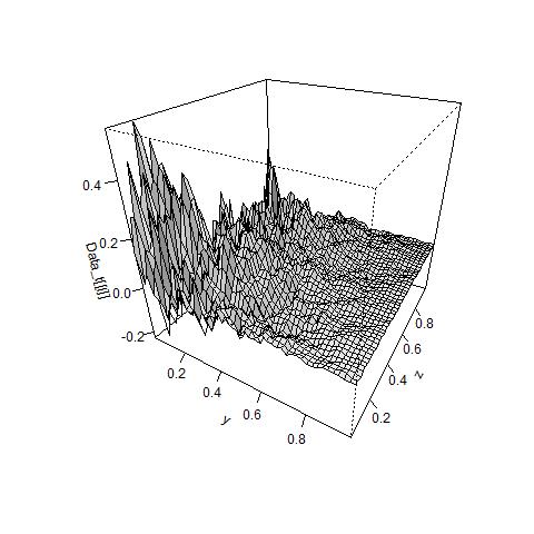
(a) Cross sections of the sample path at $t=0.5$

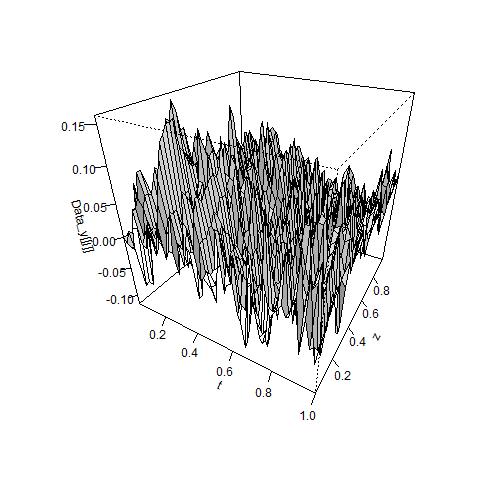
(b) Cross sections of the sample path at $y=0.5$

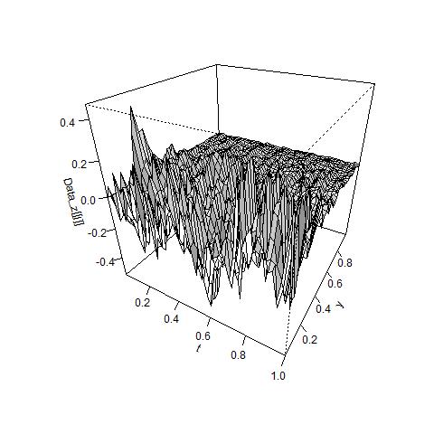
(c) Cross sections of the sample path at $z=0.5$

Figure 4. Sample path with $\theta=(0,1.5,0.2,0.2,1)$ and $\kappa=7.5$

Figure 5 is the sample path with $\theta=(0,0,0.2,0.2,1)$ and $\kappa=0$. Figure 5 shows that if $\kappa$ is close to $0$, there is not much difference between the variation of the sample path near $y=0$ and that near $y=1$.

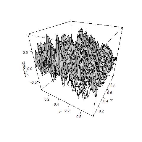
(a) Cross sections of the sample path at $t=0.5$

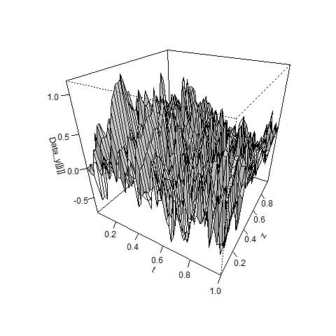
(b) Cross sections of the sample path at $y=0.5$

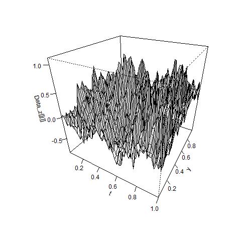
(c) Cross sections of the sample path at $z=0.5$

Figure 5. Sample path with $\theta=(0,0,0.2,0.2,1)$ and $\kappa=0$

Figure 6 is the sample path with $\theta=(0,-1.5,0.2,0.2,1)$ and $\kappa=-7.5$. Figure 6 shows that if $\kappa$ is small, the variation of the sample path is large near $y=1$ and small near $y=0$.

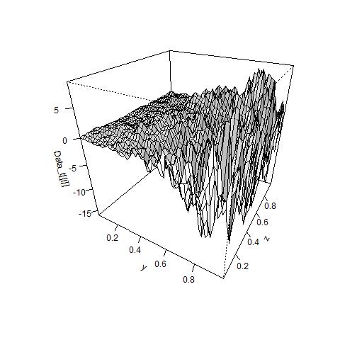
(a) Cross sections of the sample path at $t=0.5$

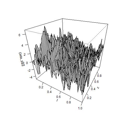
(b) Cross sections of the sample path at $y=0.5$

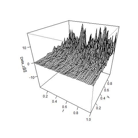
(c) Cross sections of the sample path at $z=0.5$

Figure 6. Sample path with $\theta=(0,-1.5,0.2,0.2,1)$ and $\kappa=-7.5$

characteristic of $\eta=\eta_{1}/\theta_{2}$

$\eta$ affects the variation of the sample path when $z$ is varied. Figures 7-9 are the sample paths, where $\eta$ is changed.

Figure 7 is the sample path with $\theta=(0,0.2,1.5,0.2,1)$ and $\eta=7.5$. Figure 7 shows that if $\eta$ is large, the variation of the sample path is large near $z=0$ and small near $z=1$.

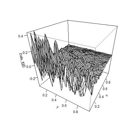
(a) Cross sections of the sample path at $t=0.5$

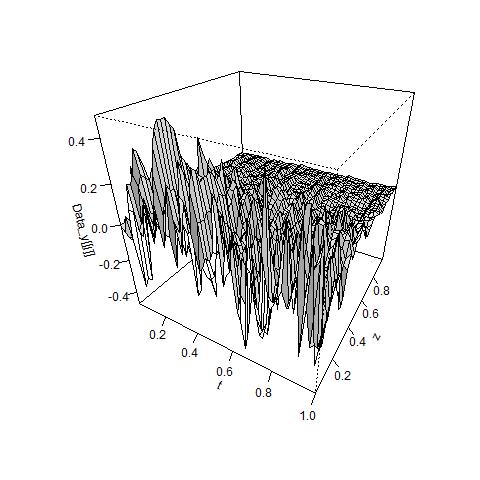
(b) Cross sections of the sample path at $y=0.5$

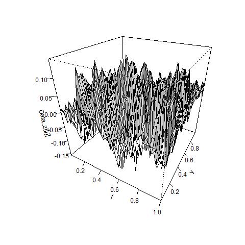
(c) Cross sections of the sample path at $z=0.5$

Figure 7. Sample path with $\theta=(0,0.2,1.5,0.2,1)$ and $\eta=7.5$

Figure 8 is the sample path with $\theta=(0,0.2,0,0.2,1)$ and $\kappa=0$. Figure 8 shows that if $\eta$ is close to $0$, there is not much difference between the variation of the sample path near $z=0$ and that near $z=1$.

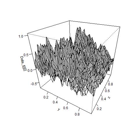
(a) Cross sections of the sample path at $t=0.5$

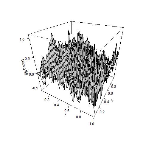
(b) Cross sections of the sample path at $y=0.5$

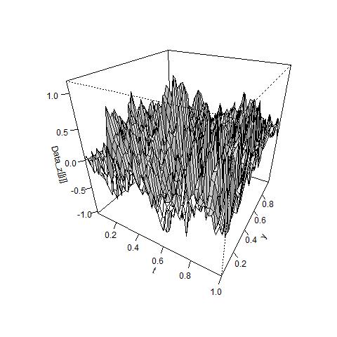
(c) Cross sections of the sample path at $z=0.5$

Figure 8. Sample path with $\theta=(0,0.2,0,0.2,1)$ and $\eta=0$

Figure 9 is the sample path with $\theta=(0,0.2,-1.5,0.2,1)$ and $\eta=-7.5$. Figure 9 shows that if $\eta$ is small, the variation of the sample path is large near $z=1$ and small near $z=0$.

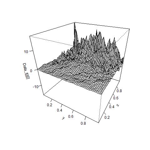
(a) Cross sections of the sample path at $t=0.5$

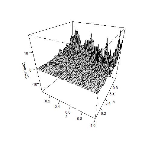
(b) Cross sections of the sample path at $y=0.5$

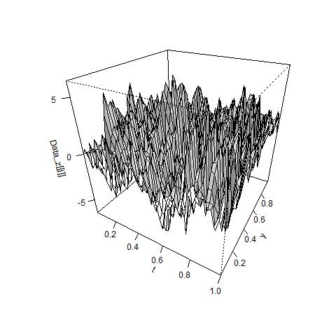
(c) Cross sections of the sample path at $z=0.5$

Figure 9. Sample path with $\theta=(0,0.2,-1.5,0.2,1)$ and $\kappa=-7.5$

References

- [1] M. Bibinger and M. Trabs. Volatility estimation for stochastic PDEs using high-frequency observations. Stochastic Processes and their Applications, 130(5):3005–3052, 2020.
- [2] C. Chong. High-frequency analysis of parabolic stochastic PDEs with multiplicative noise: Part I. arXiv preprint arXiv:1908.04145, 2019.
- [3] C. Chong. High-frequency analysis of parabolic stochastic PDEs. The Annals of Statistics, 48(2):1143–1167, 2020.
- [4] I. Cialenco. Statistical inference for SPDEs: an overview. Statistical Inference for Stochastic Processes, 21(2):309–329, 2018.
- [5] I. Cialenco, F. Delgado-Vences, and H.J. Kim. Drift estimation for discretely sampled SPDEs. Stochastics and Partial Differential Equations: Analysis and Computations, 8:895–920, 2020.
- [6] I. Cialenco and N. Glatt-Holtz. Parameter estimation for the stochastically perturbed Navier-Stokes equations. Stochastic Processes and their Applications, 121(4):701–724, 2011.
- [7] I. Cialenco and Y. Huang. A note on parameter estimation for discretely sampled SPDEs. Stochastics and Dynamics, 20(3):2050016, 2020.
- [8] V. Genon-Catalot and J. Jacod. On the estimation of the diffusion coefficient for multi-dimensional diffusion processes. Annales de l’Institut Henri Poincaré Probabilités et Statistiques, 29(1):119–151, 1993.
- [9] F. Hildebrandt. On generating fully discrete samples of the stochastic heat equation on an interval. Statistics & Probability Letters, 162:108750, 2020.
- [10] F. Hildebrandt and M. Trabs. Nonparametric calibration for stochastic reaction-diffusion equations based on discrete observations. arXiv preprint arXiv:2102.13415, 2021.
- [11] F. Hildebrandt and M. Trabs. Parameter estimation for SPDEs based on discrete observations in time and space. Electronic Journal of Statistics, 15(1):2716–2776, 2021.
- [12] M. Hübner, R. Khasminskii, and B.L. Rozovskii. Two Examples of Parameter Estimation for Stochastic Partial Differential Equations, pages 149–160. Springer New York, 1993.
- [13] Y. Kaino and M. Uchida. Parametric estimation for a parabolic linear SPDE model based on discrete observations. Journal of Statistical Planning and Inference, 211:190–220, 2020.
- [14] Y. Kaino and M. Uchida. Adaptive estimator for a parabolic linear SPDE with a small noise. Japanese Journal of Statistics and Data Science, 4:513–541, 2021.
- [15] M. Kessler. Estimation of an ergodic diffusion from discrete observations. Scandinavian Journal of Statistics, 24(2):211–229, 1997.
- [16] G.J. Lord, C.E. Powell, and T. Shardlow. An Introduction to Computational Stochastic PDEs. Cambridge Texts in Applied Mathematics. Cambridge University Press, 2014.
- [17] S. V. Lototsky. Statistical inference for stochastic parabolic equations: a spectral approach. Publicacions Matemàtiques, 53(1):3–45, 2009.
- [18] S. V. Lototsky and B.L. Rozovsky. Stochastic partial differential equations. Springer, 2017.
- [19] B. Markussen. Likelihood inference for a discretely observed stochastic partial differential equation. Bernoulli, 9:745–762, 2003.
- [20] L. Piterbarg and A. Ostrovskii. Advection and diffusion in random media: implications for sea surface temperature anomalies. Springer Science & Business Media, 1997.
- [21] G. Da Prato and J. Zabczyk. Stochastic Equations in Infinite Dimensions. Encyclopedia of Mathematics and its Applications. Cambridge University Press, 2 edition, 2014.
- [22] M. Uchida and N. Yoshida. Adaptive estimation of an ergodic diffusion process based on sampled data. Stochastic Processes and their Applications, 122(8):2885–2924, 2012.
- [23] M. Uchida and N. Yoshida. Quasi likelihood analysis of volatility and nondegeneracy of statistical random field. Stochastic Processes and their Applications, 123(7):2851–2876, 2013.