NLO QCD Corrections to ($\gamma^{*}\rightarrow Q\bar{Q}$)-Reggeon Vertex

Abstract

Next-to-leading order QCD corrections to the $\gamma^{*}\longrightarrow Q\bar{Q}-Reggeon$ vertex are calculated, where $Q\bar{Q}$ denotes a heavy quark pair $c\bar{c}$ or $b\bar{b}$. The heavy quark mass effects on the photon impact factor are found to be significant, and hence may influence the results of high energy photon-photon scattering and heavy quark pair leptoproduction. In our NLO calculation, similar to the massless case, the ultraviolate(UV) divergences are fully renormalized in the standard procedure, while the infrared (IR) divergences are regulated by the parameter $\epsilon_{IR}$ in dimensional regularization. For the process $\gamma^{*}+q\to Q\bar{Q}+q$, we calculate all NLO coefficients in terms of $\epsilon_{IR}$, and find they are enhanced due to the heavy quark mass, as compared with the light quark case, and the enhancement factors increase rapidly as the quark mass increases. This might essentially indicate the quark mass effect, in spite of the absence of real corrections that are needed in a complete NLO calculation. Moreover, unlike the $\gamma^{*}$ to massless-quark-Reggeon vertex, the results in the present work may apply to the real photon case.

PACS number(s): 12.38.Bx, 13.25.Gv, 14.40.Be

I Introduction

High energy diffractive scattering can be well described by the Pomeron exchange mechanism pom1 ; pom2 ; pom3 ; pom4 ; pom5 . Within the framework of quantum chromodynamics(QCD), the Balitskii-Fadin-Kuraev-Lipatov(BFKL) Pomeron bfkl1 ; bfkl2 ; bfkl3 , the so-called hard Pomeron, is viewed as the Green’s function of two interacting Reggeized gluons with vacuum quantum number, which is evaluated by resuming the leading energy logarithms in perturbative QCD(pQCD) applicable regime, e.g., all $(\alpha_{s}\text{ln}s)^{n}$ terms in leading logarithmic approximation(LLA) and all $\alpha_{s}(\alpha_{s}\text{ln}s)^{n}$ terms in the next-to-leading approximation(NLA). People noticed that the virtual photon-photon scattering is an ideal process virpho1 ; virpho2 to testify the BFKL predictions and hence the pQCD calculation reliability, which is highly expected in the study of strong interaction physics. The cross section $\sigma_{tot}^{\gamma^{*}\gamma^{*}}$ is calculable in the BFKL approach with relatively high precision and can be realized in experiment through a measurement of the reaction $e^{+}e^{-}\rightarrow e^{+}e^{-}+X$ by tagging the outgoing leptons at high energy electron-positron colliders, like LEP and more optimistically CEPC cepc or ILC ilc in the future. Moreover, the recently proposed electron-ion colliders like EIC eic and EicC eicc may also be good places to study the single diffractive process and hence on small-x physics at lower energies.

Till now, the leading order(LO) BFKL predictions for $e^{+}e^{-}\rightarrow e^{+}e^{-}+X$ process have been confronted to the LEP data lep1 ; lep2 ; lep3 , in which the experimental measurement is found above the two-gluon-exchange model result, while below the leading order BFKL Pomeron prediction. Now that the next-to-leading order(NLO) corrections to BFKL kernel is ready and numerically big and negative bfkl3 ; nlb2 , the higher order corrections may lower the the BFKL Pomeron exchange calculation and approach to the experimental measurement. However, in the NLO BFKL calculations, there is still a task remaining, calculating the NLO corrections to the coupling of the BFKL Pomeron and the external photons, which is called photon impact factorim1 ; im2 ; im3 .

The photon impact factor can be obtained by calculating the discontinuity of the process $\gamma^{*}+~{}reggon\longrightarrow\gamma^{*}+~{}reggon$ process in light of the optical theorem, which tells that the discontinuity is proportional to the scattering amplitude, $\gamma^{*}+~{}reggeon\longrightarrow Q\bar{Q}$, squared. The reggon, is identified with the elementary t-channel gluons. The NLO corrections to the photon impact factor with massless internal quarks were given in Ref.qiao , while here the $Q(\bar{Q})$ are massive quarks, charm or bottom quarks. In the NLO calculation, in analogous to Ref.qiao , we calculate the NLO corrections to $\gamma^{*}+~{}reggeon\longrightarrow Q\bar{Q}$ amplitude on for example left-hand side of the discontinuity line, and the leading $Q\bar{Q}g$ intermediate state on both sides of the discontinuity line. The calculation of NLO QCD correction hence proceeds in three steps: (i) calculate the NLO corrections to the $\gamma^{*}+~{}reggeon\longrightarrow Q\bar{Q}$ vertex. (ii) calculate the leading order vertex $\gamma^{*}+~{}reggeon\longrightarrow Q\bar{Q}g$, and (iii) carry out the integration over the phase space of the intermediate states. In fact, here the calculation procedure is similar to the massless case performed in Ref.qiao . In this paper, as in qiao , we give the results of the first step, in which the vertex is extracted from the scattering process $\gamma^{*}+~{}q\longrightarrow Q\bar{Q}+q$ in the high energy limit.

II Technical preliminaries

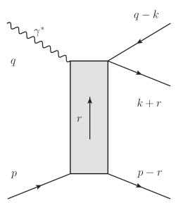
Figure 1: Kinematics of the process $\gamma^{*}+q\to Q\bar{Q}+q$.

The kinematics of the $\gamma^{*}+q\to Q\bar{Q}+q$ process is illustrated Fig.1, where $q$ and $p$ are the 4-momenta of photon and incident quark respectively. In the calculation, $\varepsilon$ represents for the polarization vector of the photon, $s$ for the collision energy of the $\gamma^{*}q$ system, and $m$ for the mass of the heavy quark. The Lorentz invariants appeared include $s=(q+p)^{2}$, $Q^{2}=-q^{2}$, $t_{a}=k^{2}$, $t_{b}=(q-k-r)^{2}$, $M^{2}=(q+r)^{2}$, $t=r^{2}$, and $x=Q^{2}/2p\cdot q$, the Bjorken scaling variable.

The momenta $k$ and $r$ can be decomposed in the Sudakov form, i.e,

$$k = \alpha q^{\prime}+\beta p+k_{\bot}\ ,$$ (1)

$$r = \frac{t}{s}q^{\prime}-\frac{t_{a}+t_{b}-2m^{2}}{s}p+r_{\bot}\ ,$$ (2)

with $q^{\prime}=q+xp$, ${q^{\prime}}^{2}=p^{2}=0$ and $\beta s=\frac{k_{\bot}^{2}+m^{2}}{1-\alpha}-Q^{2}$.

Figure 2: Feynman diagrams for the process $\gamma^{*}+q\to Q\bar{Q}+q$.

The typical Feynman diagrams for NLO corrections are shown in Fig.2. Of these diagrams, except Fig.2.14, the upper part quark-antiquark exchange diagrams are implied. For the color octet t-channel configuration, the sum of all diagrams has to be antisymmetric if we interchange quark and antiquark: $k\rightarrow q-k-r$, $\lambda\rightarrow\lambda^{\prime}$, where $\lambda$, $\lambda^{\prime}$ are the helicities of the quark and antiquark respectively. In particular, the ”box” graph shown in Fig. 3.14 has to be antisymmetric by itself. Throughout the calculation, Feynman gauge is employed, and for the t-channel gluons the metric tensor is decomposed into

$$g_{\mu\nu}=\frac{2}{s}(p_{\mu}q^{\prime}_{\nu}+p_{\nu}q^{\prime}_{\mu})+g^{\bot}_{\mu\nu}$$ (3)

as usual. Note, in practical calculations, the transverse term is not taken into account, whose contributions are suppressed by powers of $s$. We use the helicity formalism as well, and then our results can be expressed in terms of the following matrix elements similar to qiao , i.e.,

$$H_{T}^{a} = \bar{u}(k+r,\lambda)\not\!{p}\not\!{k}\not\!{\varepsilon}\;\lambda^{a}v(q-k,\lambda^{\prime})\;,$$ (4)

$$H_{\varepsilon}^{a} = \bar{u}(k+r,\lambda)\not\!{\varepsilon}\;\lambda^{a}v(q-k,\lambda^{\prime})\;,$$ (5)

$$H_{k}^{a} = \bar{u}(k+r,\lambda)\not\!{k}\;\lambda^{a}v(q-k,\lambda^{\prime})\;,$$ (6)

$$H_{p}^{a} = \bar{u}(k+r,\lambda)\not\!{p}\;\lambda^{a}v(q-k,\lambda^{\prime})\;,$$ (7)

$$H_{k\varepsilon}^{a} = \bar{u}(k+r,\lambda)\not\!{k}\not\!{\varepsilon}\;\lambda^{a}v(q-k,\lambda^{\prime})\;,$$ (8)

$$H_{p\varepsilon}^{a} = \bar{u}(k+r,\lambda)\not\!{p}\not\!{\varepsilon}\;\lambda^{a}v(q-k,\lambda^{\prime})\;,$$ (9)

$$H_{pk}^{a} = \bar{u}(k+r,\lambda)\not\!{p}\not\!{k}\;\lambda^{a}v(q-k,\lambda^{\prime})\;,$$ (10)

$$H_{m}^{a} = \bar{u}(k+r,\lambda)\;\lambda^{a}v(q-k,\lambda^{\prime}).$$ (11)

Here $\lambda^{a}$ is the generators of the color group. Note that the last four helicity matrix elements do not exist in qiao , which always come up with the factor of $m$.

Take high energy limit in the calculation, where

$$t,Q^{2},t_{a},t_{b},M^{2},m^{2}\ll s,$$ (12)

and do not impose any restrictions on the remaining invariants, we then obtain the following amplitude

$$T=g^{2}\;T^{(0)}+g^{4}\;T^{(1)},$$ (13)

with

$$T^{(0)}=\Gamma_{\gamma^{*}\to q\bar{q}}^{(0),a}\;\frac{2s}{t}\;\Gamma_{qq}^{(0),a},$$ (14)

and

$$\Gamma_{qq}^{(0),a} = \frac{1}{s}\bar{u}(p-r,\,\lambda^{\prime})\not\!{q}^{\prime}\lambda^{a}u(p,\,\lambda)\ .$$ (15)

The only unknown piece of the NLO amplitude is $T^{(1)}$, which corresponds to the processes in Fig.2.1 - 2.14 and will be calculated analytically in the following.

III Calculation methods

The method we use in our calculation will be briefly described in the following before presenting the explicit results.

In our calculation the MATHEMATICA package FeynArts feynarts is applied to generate the Feynman diagrams and amplitudes that are relevant to our process. We use FeynCalc feyncalc to calculate and simplify the amplitudes. Color in the t-channel is projected onto the antisymmetric octet as done in qiao . After simplifying the Dirac matrix and employing the Dirac equation of motion, we express the amplitudes as the combination of helicity matrix elements and Passarino-Veltman integrals. For integrals that contain divergences, we separate the divergence part from the finite one. The high energy limit is taken through out our calculation, i.e. $t,Q^{2},t_{a},t_{b},M^{2},m^{2}\ll s$.

In this work an extra scale $m$ exists in comparison to qiao , and it is too lengthy and redundancy to turn all the Passarino-Veltman integrals into scalar integrals or logarithms and dilogarithms functions. For amplitudes that do not contain divergences and high energy scale $s$, we express them as the combination of Passarino-Veltman integrals and helicity matrix elements. The numerical values of these integrals will be evaluated by Looptools looptools . For the pentagon diagram Fig.2.13, the reduction method given in denner is employed to reduce the corresponding integrals to box integrals. In the end we find our result agrees with that in qiao when taking the $m\rightarrow 0$ limit.

IV Analytic Results

The NLO amplitudes in $T^{(1)}$ of our concern can be expressed in terms of different diagrams:

$$T^{(1)} = \sum_{i=1}^{13}(A_{i}+\bar{A}_{i})+A_{14}\ .$$ (16)

Here, the subscripts $i$ denote diagrams in Fig.2, and the amplitudes $\bar{A}_{i}$ represent those with quark-antiquark interchange in ${A}_{i}$.

IV.1 Results of two- and three-point diagrams

We categorize the diagrams similar to qiao . The results of Figs.2.1 and its conjugate one are given below, which are split into divergent and finite parts in $\mathrm{\overline{MS}}$ scheme:

$$A_{1}\, =\,\frac{N_{c}}{2}\frac{ee_{f}}{(4\pi)^{2-\epsilon}}\frac{2}{t(t_{a}-m^{2})}\Gamma_{qq}^{(0),a}\bigg{\{}\frac{3(H_{T}^{a}+mH_{p\varepsilon}^{a})c_{\Gamma}}{\epsilon}+H_{T}^{a}\big{[}6m^{2}C_{0}(1)+12C_{00}(1)_{fin}$$

$$+(5m^{2}-2t+3t_{a})C_{1}(1)+(3m^{2}-t+t_{a})C_{2}(1)+2t_{a}C_{11}(1)+2(m^{2}-t+t_{a})C_{12}(1)$$

$$+2m^{2}C_{22}(1)-2\big{]}+\alpha sH_{\varepsilon}^{a}\big{[}2m^{2}C_{1}(1)+(3m^{2}-t_{a})C_{2}(1)+2t_{a}C_{11}(1)+2m^{2}C_{22}(1)$$

$$+2(t_{a}+m^{2})C_{12}(1)\big{]}+mH_{p\varepsilon}^{a}\big{[}3(t_{a}+m^{2})C_{0}(1)+12C_{00}(1)_{fin}+2(m^{2}-t+3t_{a})C_{1}(1)$$

$$+(3m^{2}-2t+5t_{a})C_{2}(1)+2t_{a}C_{11}(1)+2(m^{2}-t+t_{a})C_{12}(1)+2m^{2}C_{22}(1)-2\big{]}$$

$$+2\alpha smH_{k\varepsilon}^{a}\big{[}C_{1}(1)+C_{2}(1)+C_{11}(1)+2C_{12}(1)+C_{22}(1)\big{]}\bigg{\}}\ .$$ (17)

Here $C_{i}(1)=C_{i}(t_{a},t,m^{2},m^{2},0,0)$ with $i$ the coefficient index. The definitions of all the loop integrals such as $C_{0}$, $C_{ij}$,$D_{0}$, $D_{i,j,k}$ are standard and given in the Appendix for reference. The subindex $fin$ means the finite part of the loop integrals. Note, the above result does not contain any infrared divergences, while the ultraviolet divergence remains only in $C_{00}(1)$, which can be properly regulated. Numerical evaluation of the finite part may be performed by means of LoopTools looptools in $\mathrm{\overline{MS}}$ scheme. The $C_{i}$ functions can be reduced into a certain scalar one-loop integrals and then expressed as the combination of logarithm and dilogarithm functions. Nevertheless, such kind of reduction may yield a lengthy result and hard to read. Due to this reason, we do not perform further reduction on $C_{i}$ functions, its numerical evaluations are carried by LoopTools directly.

The result of the conjugate diagram of Figs.2.1 can be expressed as

$$\bar{A}_{1}\, =\,\frac{N_{c}}{2}\frac{ee_{f}}{(4\pi)^{2-\epsilon}}\frac{2}{t(t_{b}-m^{2})}\Gamma_{qq}^{(0),a}\bigg{\{}\frac{3(H_{T}^{a}+mH_{p\varepsilon}^{a}-sH_{\varepsilon}^{a}+2(H_{k}^{a}-mH_{m}^{a})\varepsilon\cdot p+2H_{p}^{a}\varepsilon\cdot r)c_{\Gamma}}{\epsilon}$$

$$+(H_{T}^{a}+2H_{p}^{a}\varepsilon\cdot r+2H_{k}^{a}\varepsilon\cdot p)\big{[}6m^{2}C_{0}(\bar{1})+12C_{00}(\bar{1})_{fin}+2(3m^{2}-t+t_{b})C_{1}(\bar{1})$$

$$+(5m^{2}-2t+3t_{b}^{2})C_{2}(\bar{1})+2m^{2}C_{11}(\bar{1})+2(m^{2}-t+t_{b})C_{12}(\bar{1})+2t_{b}C_{22}(\bar{1})-2\big{]}$$

$$+sH_{\varepsilon}^{a}\big{[}-6m^{2}C_{0}(\bar{1})+(3(\alpha-3)m^{2}+2t-(1+\alpha)t_{b})C_{1}(\bar{1})-12C_{00}(\bar{1})_{fin}$$

$$+((2\alpha-7)m^{2}+2t-3t_{b})C_{2}(\bar{1})+2(\alpha-2)m^{2}C_{11}(\bar{1})+2(\alpha-2)t_{b}C_{22}(\bar{1})$$

$$+2((\alpha-2)m^{2}+t+(\alpha-2)t_{b})C_{12}(\bar{1})+2\big{]}$$

$$+2(\alpha-1)sm(H_{k\varepsilon}^{a}+H_{m}^{a}\varepsilon\cdot r)\big{[}C_{1}(\bar{1})+C_{2}(\bar{1})+C_{11}(\bar{1})+2C_{12}(\bar{1})+C_{22}(\bar{1})\big{]}$$

$$+m(H_{p\varepsilon}^{a}-2\varepsilon\cdot pH_{m}^{a})\big{[}(9m^{2}-3t_{b})C_{0}(\bar{1})+12C_{00}(\bar{1})_{fin}+(9m^{2}-2t-t_{b})C_{1}(\bar{1})$$

$$+2(4m^{2}-t)C_{2}(\bar{1})+2m^{2}C_{11}(\bar{1})+2(m^{2}-t+t_{b})C_{12}(\bar{1})+2t_{b}C_{22}(\bar{1})-2\big{]}\bigg{\}}\ .$$ (18)

Here, $C_{i}(\bar{1})=C_{i}(m^{2},t,t_{b},m^{2},0,0)$.

The calculation procedure of Fig.2.4 is similar to that of Fig.1, and its result reads:

$$A_{4}\, =\,-\frac{1}{2N_{c}}\frac{ee_{f}}{(4\pi)^{2-\epsilon}}\frac{4}{t(t_{a}-m^{2})}\Gamma_{qq}^{(0),a}\bigg{\{}\frac{(H_{T}^{a}+mH_{p\varepsilon}^{a})c_{\Gamma}}{2\epsilon}+H_{T}^{a}\big{[}(m^{2}-t+t_{a})C_{0}(4)$$

$$+(3m^{2}-t+t_{a})C_{1}(4)+(2m^{2}-t+2t_{a})C_{2}(4)+2C_{00}(4)_{fin}+m^{2}C_{11}(4)$$

$$+(m^{2}-t+t_{a})C_{12}(4)+t_{a}C_{22}(4)-1\big{]}+\alpha sH_{\varepsilon}^{a}\big{[}(m^{2}-t_{a})C_{0}(4)-t_{a}C_{1}(4)$$

$$+(m^{2}-2t_{a})2C_{2}(4)-m^{2}C_{11}(4)-(t_{a}+m^{2})C_{12}(4)-t_{a}C_{22}(4)\big{]}$$

$$+mH_{p\varepsilon}^{a}\big{[}(2t_{a}-t)C_{0}(4)+(2m^{2}-t+2t_{a})C_{1}(4)+(m^{2}-t+3t_{a})C_{2}(4)$$

$$+2C_{00}(4)_{fin}+m^{2}C_{11}(4)+(m^{2}-t+t_{a})C_{12}(4)+t_{a}C_{22}(4)-1\big{]}$$

$$-\alpha smH_{k\varepsilon}^{a}\big{[}C_{1}(4)+C_{2}(4)+C_{11}(4)+2C_{12}(4)+C_{22}(4)\big{]}\bigg{\}}\ .$$ (19)

where $C_{i}(4)=C_{i}(m^{2},t,t_{a},0,m^{2},m^{2})$.

The result of the conjugate diagram of Fig.2.4 is:

$$\bar{A}_{4}\, =\,-\frac{1}{2N_{c}}\frac{ee_{f}}{(4\pi)^{2-\epsilon}}\frac{4}{t(t_{b}-m^{2})}\Gamma_{qq}^{(0),a}\bigg{\{}$$

$$\frac{(H_{T}^{a}+mH_{p\varepsilon}^{a}-sH_{\varepsilon}^{a}+2(H_{k}^{a}-mH_{m}^{a})\varepsilon\cdot p+2H_{p}^{a}\varepsilon\cdot r)c_{\Gamma}}{2\epsilon}$$

$$+H_{T}^{a}\big{[}(m^{2}-t+t_{b})C_{0}(\bar{4})+(3m^{2}-t+t_{b})C_{1}(\bar{4})+(2m^{2}-t+2t_{b})C_{2}(\bar{4})$$

$$+2C_{00}(\bar{4})_{fin}+m^{2}C_{11}(\bar{4})+(m^{2}-t+t_{b})C_{12}(\bar{4})+t_{b}C_{22}(\bar{4})-1\big{]}$$

$$+sH_{\varepsilon}^{a}\big{[}((\alpha-2)m^{2}+t-\alpha t_{b})C_{0}(\bar{4})+(t-3m^{2}-\alpha t_{b})C_{1}(\bar{4})$$

$$+((\alpha-3)m^{2}+t-2\alpha t_{b})C_{2}(\bar{4})-2C_{00}(\bar{4})_{fin}-\alpha m^{2}C_{11}(\bar{4})$$

$$+(t-\alpha m^{2}-\alpha t_{b})C_{12}(\bar{4})-\alpha t_{b}C_{22}(\bar{4})+1\big{]}$$

$$+2(H_{k}^{a}\varepsilon\cdot p+H_{p}^{a}\varepsilon\cdot r)\big{[}(m^{2}-t+t_{b})C_{0}(\bar{4})+2C_{00}(\bar{4})_{fin}$$

$$+(3m^{2}-t+t_{b})C_{1}(\bar{4})+(2m^{2}-t+2t_{b})C_{2}(\bar{4})+m^{2}C_{11}(\bar{4})$$

$$+(m^{2}-t+t_{b})C_{12}(\bar{4})+t_{b}C_{22}(\bar{4})-1\big{]}$$

$$+m(H_{p\varepsilon}^{a}+2H_{m}^{a}\varepsilon\cdot p)\big{[}(2m^{2}-t)C_{0}(\bar{4})+(4m^{2}-t)C_{1}(\bar{4})+(3m^{2}-t+t_{b})C_{2}(\bar{4})$$

$$+2C_{00}(\bar{4})_{fin}+m^{2}C_{11}(\bar{4})+(m^{2}-t+t_{b})C_{12}(\bar{4})+t_{b}C_{22}(\bar{4})-1\big{]}$$

$$+(1-\alpha)m(H_{k\varepsilon}^{a}+2H_{m}^{a}\varepsilon\cdot r)\big{[}C_{1}(\bar{4})+C_{2}(\bar{4})+C_{11}(\bar{4})+2C_{12}(\bar{4})+C_{22}(\bar{4})\big{]}\bigg{\}}.$$ (20)

with $C_{i}(\bar{4})=C_{i}(m^{2},t,t_{b},0,m^{2},m^{2})$.

The Fig.2.5 and Fig.2.6 diagrams belong to the NLO corrections to the lower vertex $\Gamma_{qq}^{(1),a}$. Their results are

$$A_{5}\, =\,-N_{c}\frac{ee_{f}}{(4\pi)^{2-\epsilon}}\frac{2}{t(t_{a}-m^{2})}\Gamma_{qq}^{(0),a}(H_{T}^{a}+mH_{p\varepsilon}^{a})c_{\Gamma}\bigg{\{}\frac{(-t)^{-\epsilon}}{2\epsilon}+1\bigg{\}},$$ (21)

and

$$A_{6}\, =\,\frac{1}{2N_{c}}\frac{ee_{f}}{(4\pi)^{2-\epsilon}}\frac{2}{t(t_{a}-m^{2})}\Gamma_{qq}^{(0),a}(H_{T}^{a}+mH_{p\varepsilon}^{a})c_{\Gamma}(-t)^{-\epsilon}\bigg{\{}\frac{2}{\epsilon^{2}}+\frac{3}{\epsilon}+8\bigg{\}}\ .$$ (22)

In the zero mass limit, it is obvious that these two amplitudes are just the eqs. $(35)$ and $(36)$ in qiao .

Figs.2.7 - 2.9 contribute to both the upper and lower vertices, and we find

$$A_{7+8}\, =\,\frac{ee_{f}}{(4\pi)^{2-\epsilon}}\frac{2N_{c}c_{\Gamma}(-t)^{-\epsilon}}{t(t_{a}-m^{2})}\Gamma_{qq}^{(0),a}(H_{T}^{a}+mH_{p\varepsilon}^{a})\bigg{(}\frac{5}{3\epsilon}+\frac{31}{9}\bigg{)},$$ (23)

and

$$A_{9}\, =\,-n_{f}\frac{ee_{f}}{(4\pi)^{2-\epsilon}}\frac{2c_{\Gamma}(-t)^{-\epsilon}}{t(t_{a}-m^{2})}\Gamma_{qq}^{(0),a}(H_{T}^{a}+mH_{p\varepsilon}^{a})\bigg{(}\frac{2}{3\epsilon}+\frac{10}{9}\bigg{)}\ .$$ (24)

The results of conjugate diagrams of Fig.2.5 - 2.9 can readily be obtained by substituting $(H_{T}^{a}+mH_{p\varepsilon}^{a})$ with $(H_{T}^{a}+mH_{p\varepsilon}^{a}-sH_{\varepsilon}^{a}+2(H_{k}^{a}-mH_{m}^{a})\varepsilon\cdot p+2H_{p}^{a}\varepsilon\cdot r)$ and making the replacement $t_{a}\rightarrow t_{b}$.

The result of vertex correction diagram Fig.2.10 can be expressed as follows:

$$A_{10}\, =\,-\frac{C_{F}ee_{f}}{(4\pi)^{2-\epsilon}}\frac{4}{t(t_{a}-m^{2})}\Gamma_{qq}^{(0),a}\bigg{\{}\frac{-(H_{T}^{a}+mH_{p\varepsilon}^{a})c_{\Gamma}}{2\epsilon}+H_{T}^{a}\big{[}m^{2}C_{0}(10)+Q^{2}C_{2}(10)$$

$$+(m^{2}+Q^{2}+t_{a})C_{1}(10)-2C_{00}(10)_{fin}-m^{2}C_{11}(10)+(Q^{2}+t_{a}-m^{2})C_{12}(10)$$

$$+Q^{2}C_{22}(10)+1\big{]}+mH_{p\varepsilon}^{a}\big{[}m^{2}C_{0}(10)+(Q^{2}+2t_{a})C_{1}(10)+Q^{2}C_{2}(10)$$

$$-2C_{00}(10)_{fin}-m^{2}C_{11}(10)+(Q^{2}-m^{2}+t_{a})C_{12}(10)+Q^{2}C_{22}(10)+1\big{]}$$

$$+2\varepsilon\cdot k\big{[}(m(2mH_{p}^{a}+H_{pk}^{a})-t_{a}H_{p}^{a})C_{1}(10)+m(mH_{p}^{a}+H_{pk}^{a})C_{11}(10)$$

$$+H_{p}^{a}(m^{2}-t_{a})C_{12}(10)\big{]}\bigg{\}}.$$ (25)

Here $C_{i}(10)=C_{i}(m^{2},t_{a},-Q^{2},m^{2},0,m^{2})$.

The NLO amplitude of the conjugate diagram of Fig.2.10 is

$$\bar{A}_{10}\, =\,-\frac{C_{F}ee_{f}}{(4\pi)^{2-\epsilon}}\frac{4}{t(t_{b}-m^{2})}\Gamma_{qq}^{(0),a}\bigg{\{}$$

$$-\frac{(H_{T}^{a}+mH_{p\varepsilon}^{a}-sH_{\varepsilon}^{a}+2(H_{k}^{a}-mH_{m}^{a})\varepsilon\cdot p+2H_{p}^{a}\varepsilon\cdot r)c_{\Gamma}}{2\epsilon}$$

$$+(H_{T}^{a}-sH_{\varepsilon}^{a}+2H_{k}^{a}\varepsilon\cdot p)\big{[}m^{2}C_{0}(\bar{10})+(m^{2}+Q^{2}+t_{b})C_{1}(\bar{10})+Q^{2}C_{2}(\bar{10})$$

$$-2C_{00}(\bar{10})_{fin}-m^{2}C_{11}(\bar{10})+(Q^{2}-m^{2}+t_{b})C_{12}(\bar{10})+Q^{2}C_{22}(\bar{10})+1\big{]}$$

$$+mH_{p\varepsilon}^{a}\big{[}m^{2}C_{0}(\bar{10})+(2m^{2}+Q^{2})C_{1}(\bar{10})+Q^{2}C_{2}(\bar{10})-2C_{00}(\bar{10})_{fin}-m^{2}C_{11}(\bar{10})$$

$$+(Q^{2}-m^{2}+t_{b})C_{12}(\bar{10})+Q^{2}C_{22}(\bar{10})+1\big{]}+2H_{pk}^{a}\big{[}C_{1}(\bar{10})+C_{11}(\bar{10})\big{]}\times$$

$$(\varepsilon\cdot r+\varepsilon\cdot k)+2mH_{p}^{a}\big{[}((2m^{2}-t_{b})C_{1}(\bar{10})+m^{2}C_{11}(\bar{10})+(m^{2}-t_{b})C_{12}(\bar{10}))\varepsilon\cdot k$$

$$+(m^{2}C_{0}(\bar{10})+(3m^{2}+Q^{2})C_{1}(\bar{10})+Q^{2}C_{2}(\bar{10})-2C_{00}(\bar{10})_{fin}+Q^{2}C_{12}(\bar{10})$$

$$+Q^{2}C_{22}(\bar{10})+1)\varepsilon\cdot r\big{]}+2mH_{m}^{a}\big{[}(-m^{2}C_{0}(\bar{10})-(2m^{2}+Q^{2})C_{1}(\bar{10})-Q^{2}C_{2}(\bar{10})$$

$$+2C_{00}(\bar{10})_{fin}+m^{2}C_{11}(\bar{10})+(m^{2}-Q^{2}-t_{b})C_{12}(\bar{10})-Q^{2}C_{22}(\bar{10})-1)\varepsilon\cdot p$$

$$-s(C_{1}(\bar{10})+C_{11}(\bar{10}))(\varepsilon\cdot r+\varepsilon\cdot k)\big{]}\bigg{\}}.$$ (26)

with $C_{i}(\bar{10})=C_{i}(m^{2},t_{b},-Q^{2},m^{2},0,m^{2})$.

The result of the quark self-energy diagram Fig.2.11 is

$$A_{11}\, =\,\frac{ee_{f}}{(4\pi)^{2-\epsilon}}\frac{2C_{F}c_{\Gamma}}{t(t_{a}-m^{2})^{2}}\Gamma_{qq}^{(0),a}\bigg{\{}\frac{(7m^{2}-t_{a})H_{T}^{a}+2(t_{a}+2m^{2})mH_{p\varepsilon}^{a}}{\epsilon}+\ln(m^{2})[$$

$$(t_{a}-7m^{2})H_{T}^{a}-2(t_{a}+2m^{2})mH_{p\varepsilon}^{a}]+\frac{4t_{a}(t_{a}+m^{2})mH_{p\varepsilon}^{a}-(m^{4}-10t_{a}m^{2}+t_{a}^{2})H_{T}^{a}}{t_{a}}$$

$$+\frac{\ln(1-\frac{t_{a}}{m^{2}})(t_{a}-m^{2})((m^{4}-6t_{a}m^{2}+t_{a}^{2})H_{T}^{a}-2t_{a}(t_{a}+m^{2})mH_{p\varepsilon}^{a})}{t_{a}^{2}}\bigg{\}}.$$ (27)

and the amplitude of the conjugate diagram of Fig.3.11 reads

$$\bar{A}_{11}\, =\,\frac{ee_{f}}{(4\pi)^{2-\epsilon}}\frac{2C_{F}c_{\Gamma}}{t(t_{b}-m^{2})^{2}}\Gamma_{qq}^{(0),a}\bigg{\{}\frac{(7m^{2}-t_{b})(H_{T}^{a}-sH_{\epsilon}^{a}+2H_{k}^{a}\varepsilon\cdot p+2H_{p}^{a}\varepsilon\cdot r)}{\epsilon}$$

$$+\frac{2(5m^{2}-2t_{b})m(H_{p\varepsilon}^{a}-2H_{m}^{a}\varepsilon\cdot p)}{\epsilon}+\frac{1}{t_{a}}\big{[}(H_{T}^{a}-sH_{\epsilon}^{a}+2H_{k}^{a}\varepsilon\cdot p+2H_{p}^{a}\varepsilon\cdot r$$

$$)(-t_{b}(7m^{2}-t_{b})\ln(m^{2})-\frac{m^{2}-t_{b}}{t_{b}}(m^{4}-6m^{2}t_{b}+t_{b}^{2})\ln(\frac{m^{2}-t_{b}}{m^{2}})$$

$$-m^{4}+10m^{2}t_{b}-t_{b}^{2})+2m(H_{p\varepsilon}^{a}-2H_{m}^{a}\varepsilon\cdot p)(-t_{b}(5m^{2}-2t_{b})\ln(m^{2})$$

$$-\frac{m^{2}-t_{b}}{t_{b}}(m^{4}-5m^{2}t_{b}+2t_{b}^{2})\ln(\frac{m^{2}-t_{b}}{m^{2}})-m^{4}+8m^{2}t_{b}-3t_{b}^{2})\big{]}\bigg{\}}\ .$$ (28)

IV.2 The Box diagrams

Here, we present the results of box diagrams. In the calculation of diagrams Fig.2.2 and Fig.2.3, the four-point integrals have to be concerned. After taking the high energy limit and eliminating the $s$ suppressed terms, in the end the results turn out to be quit simple, that is

$$A_{2+3}\, =\,\frac{ee_{f}N_{c}}{(4\pi)^{2-\epsilon}}\frac{c_{\Gamma}}{t(t_{a}-m^{2})}\Gamma_{qq}^{(0),a}(H_{T}^{a}+mH_{p\varepsilon}^{a})\big{\{}\frac{(-t)^{-\epsilon}}{\epsilon^{2}}-\frac{3(m^{2})^{-\epsilon}}{2\epsilon^{2}}+\frac{(m^{2})^{-\epsilon}}{\epsilon}\big{(}$$

$$\ln(-\frac{\alpha s}{m^{2}})+\ln(\frac{\alpha s}{m^{2}})+\ln(\frac{-t}{m^{2}})-\ln(1-\frac{t_{a}}{m^{2}})\big{)}-\ln(-\frac{t}{m^{2}})\big{[}\ln(-\frac{\alpha s}{m^{2}})+\ln(\frac{\alpha s}{m^{2}})\big{]}$$

$$-\ln(1-\frac{t_{a}}{m^{2}})^{2}-\frac{3\pi^{2}}{4}+C_{0}(1)\big{\}}.$$ (29)

Here, $C_{0}(1)=C_{0}(t_{a},t,m^{2},m^{2},0,0)$, as in the $A_{1}$.

The results of diagrams conjugating to Fig.2.2 and Fig.2.3 can be obtained by taking the following replacements:
$t_{a}\rightarrow t_{b}$, $\alpha\rightarrow 1-\alpha$, $(H_{T}^{a}+mH_{p\varepsilon}^{a})\rightarrow(H_{T}^{a}+mH_{p\varepsilon}^{a}-sH_{\varepsilon}^{a}+2(H_{k}^{a}-mH_{m}^{a})\varepsilon\cdot p+2H_{p}^{a}\varepsilon\cdot r)$.

Note that there are $\text{ln}s$ terms in the amplitudes of Figs.2.2 and 2.3, and also their conjugate partners.

Next, we give the result of adjacent box as shown in Fig.2.12.

$$A_{12}\, =\,\Gamma_{qq}^{(0),a}\frac{2s}{t}\bigg{(}\frac{ee_{f}}{s}\bigg{)}\bigg{(}-\frac{1}{2N_{c}}\bigg{)}\frac{2}{(4\pi)^{2-\epsilon}}\bigg{\{}\frac{c_{\Gamma}}{\epsilon}A_{12}^{-1}+A_{12}^{0}\bigg{\}}\ .$$ (30)

in which the divergent part $A_{12}^{-1}$ is

$$A_{12}^{-1}\, =\,-(H_{T}^{a}+mH_{p\varepsilon}^{a})\frac{M^{2}x_{r}\ln(x_{r})}{m^{2}(1-x_{r}^{2})},$$ (31)

with

$$x_{r}=-\frac{1-\sqrt{1-\frac{4m^{2}}{2m^{2}+M^{2}}}}{1+\sqrt{1-\frac{4m^{2}}{2m^{2}+M^{2}}}}\ ,$$ (32)

and $M^{2}=(q+r)^{2}$, defined in the above paragraph.

The finite term $A_{12}^{0}$ is given in the Appendix. The amplitude of the conjugate diagram of Fig.2.12 goes as

$$\bar{A}_{12}\, =\,\Gamma_{qq}^{(0),a}\frac{2s}{t}\bigg{(}\frac{ee_{f}}{s}\bigg{)}\bigg{(}-\frac{1}{2N_{c}}\bigg{)}\frac{2}{(4\pi)^{2-\epsilon}}\bigg{\{}\frac{c_{\Gamma}}{\epsilon}\bar{A}_{12}^{-1}+\bar{A}_{12}^{0}\bigg{\}}\ ,$$ (33)

where the divergent term

$$\bar{A}_{12}^{-1}=-\frac{M^{2}x_{r}\ln(x_{r})}{m^{2}(1-x_{r}^{2})}\big{[}H_{T}^{a}+mH_{p\varepsilon}^{a}-sH_{\varepsilon}^{a}+2(H_{k}^{a}-mH_{m}^{a})\varepsilon\cdot p+2H_{p}^{a}\varepsilon\cdot r\big{]}\ .$$ (34)

The finite piece is also given in the Appendix.

The opposite box diagram Fig.2.14 does not contain any divergence, its lengthy analytic expression is presented in the Appendix.

IV.3 The Pentagon diagram

In this subsection we deal with the pentagon diagram Fig.2.13. The calculation procedure is complicated, and is performed by computer algebra. Due to the fact that the integrals depend upon the large scale $s$, they can be greatly simplified in the high energy limit. The results are as follows:

$$A_{13}\, =\,\Gamma_{qq}^{(0),a}\frac{N_{c}}{2}\frac{ee_{f}}{t(4\pi)^{2-\epsilon}}\bigg{\{}\frac{1}{\epsilon^{2}}A_{13}^{(-2)}+\frac{1}{\epsilon}A_{13}^{(-1)}+\frac{A_{13}^{(0)}}{\Delta}\bigg{\}}\ .$$ (35)

Here,

$$\Delta\, =\,\alpha(\alpha-1)m^{4}-m^{2}(t+\alpha(\alpha-1)(t_{a}+t_{b}))+\alpha(\alpha-1)(Q^{2}t+t_{a}t_{b})\ ,$$ (36)

$$A_{13}^{(-2)}\, =\,\bigg{\{}-(H_{T}^{a}+mH_{p\varepsilon}^{a})\big{[}\frac{1}{t_{a}-m^{2}}+\frac{1}{t_{b}-m^{2}}\big{]}+\frac{sH_{\varepsilon}^{a}-2(H_{k}^{a}-mH_{m}^{a})\varepsilon\cdot p-2H_{p}^{a}\varepsilon\cdot r}{t_{b}-m^{2}}\bigg{\}}\ ,$$ (37)

and

$$A_{13}^{(-1)}\, =\,2\bigg{\{}(H_{T}^{a}+mH_{p\varepsilon}^{a})\big{[}\ln(m)(\frac{1}{t_{a}-m^{2}}+\frac{1}{t_{b}-m^{2}})+\frac{\ln(1-\frac{t_{a}}{m^{2}})}{t_{a}-m^{2}}+\frac{\ln(1-\frac{t_{b}}{m^{2}})}{t_{b}-m^{2}}$$

$$+\frac{(t_{b}-t_{a})\ln(\frac{\alpha-1}{\alpha})}{(t_{a}-m^{2})(t_{b}-m^{2})}\big{]}-\frac{sH_{\varepsilon}^{a}-2(H_{k}^{a}-mH_{m}^{a})\varepsilon\cdot p-2H_{p}^{a}\varepsilon\cdot r}{t_{b}-m^{2}}\ln\bigg{(}\frac{(t_{a}-m^{2})\alpha}{m(1-\alpha)}\bigg{)}\bigg{\}}\ .$$ (38)

The finite piece $A_{13}^{(0)}$ in (35) is listed in the Appendix. Note, we can reproduce the massless result qiao when taking the $m\rightarrow 0$ limit in above expressions.

We can obtain the amplitude of the conjugate diagram of Fig.2.13 by replacing $s\rightarrow-s$ in the $D_{0}(1),D_{0}(2),D_{0}(3),D_{0}(4)$ and $D_{i}(14)\rightarrow-D_{i}(14)$. With there replacements one can easily find that the energy dependence $\text{ln}~{}s$ terms in Fig.2.13 cancel the terms in its conjugate diagram. Therefore, the energy dependence terms merely come from $A_{2+3}+\bar{A}_{2+3}$.

V Renormalization

The results of our concerned process contain both infrared and ultraviolet divergences. The ultraviolet divergences may be renormalized via standard procedure, i.e. canceled by counter terms, in modified minimal subtraction ($\overline{MS}$) scheme here. The infrared divergences may be canceled out when the soft gluon radiation process $\gamma^{*}+~{}reggeon\longrightarrow Q\bar{Q}g$ is taken into account.

The ultraviolet divergences exist only in the self-energy and triangle diagrams, which are

$$A_{1}^{UV} = \frac{ee_{f}}{(4\pi)^{2-\epsilon}}\frac{2(H_{T}^{a}+mH_{p\varepsilon}^{a})}{t(t_{a}-m^{2})}\Gamma_{qq}^{(0),a}\ \frac{3N_{c}c_{\Gamma}}{2\epsilon_{UV}},$$ (39)

$$A_{4}^{UV} = \frac{ee_{f}}{(4\pi)^{2-\epsilon}}\frac{2(H_{T}^{a}+mH_{p\varepsilon}^{a})}{t(t_{a}-m^{2})}\Gamma_{qq}^{(0),a}(-\frac{c_{\Gamma}}{2N_{c}\epsilon_{UV}})\ ,$$ (40)

$$A_{5}^{UV} = \frac{ee_{f}}{(4\pi)^{2-\epsilon}}\frac{2(H_{T}^{a}+mH_{p\varepsilon}^{a})}{t(t_{a}-m^{2})}\Gamma_{qq}^{(0),a}\frac{3N_{c}c_{\Gamma}}{2\epsilon_{UV}}\ ,$$ (41)

$$A_{6}^{UV} = \frac{ee_{f}}{(4\pi)^{2-\epsilon}}\frac{2(H_{T}^{a}+mH_{p\varepsilon}^{a})}{t(t_{a}-m^{2})}\Gamma_{qq}^{(0),a}(-\frac{c_{\Gamma}}{2N_{c}\epsilon_{UV}})\ ,$$ (42)

$$A_{7+8+9}^{UV} = \frac{ee_{f}}{(4\pi)^{2-\epsilon}}\frac{2(H_{T}^{a}+mH_{p\varepsilon}^{a})}{t(t_{a}-m^{2})}\Gamma_{qq}^{(0),a}\frac{c_{\Gamma}}{\epsilon_{UV}}(\frac{5}{3}N_{c}-\frac{2}{3}n_{f})\ ,$$ (43)

$$A_{10}^{UV} = \frac{ee_{f}}{(4\pi)^{2-\epsilon}}\frac{2(H_{T}^{a}+mH_{p\varepsilon}^{a})}{t(t_{a}-m^{2})}\Gamma_{qq}^{(0),a}\frac{c_{\Gamma}}{\epsilon_{UV}}C_{F}\ ,$$ (44)

and

$$A_{11}^{UV} = \frac{ee_{f}}{(4\pi)^{2-\epsilon}}\frac{2}{t(t_{a}-m^{2})^{2}}\Gamma_{qq}^{(0),a}\frac{c_{\Gamma}}{\epsilon_{UV}}2C_{F}((7m^{2}-t_{a})H_{T}^{a}+2(t_{a}+2m^{2})mH_{p\varepsilon}^{a})\ .$$ (45)

For the ultraviolet divergence discussed above, when taking the massless limit we can find it is in agreement with the result in qiao . We denote $Z_{2},Z_{3},Z_{m},Z_{g}$ as the quark-field, gluon-field, mass, and coupling renormalization constants, respectively. Note, in our calculation the renormalization constants $Z_{2}$ and $Z_{m}$ are defined in on-shell Scheme, while $Z_{3}$ and $Z_{g}$ are given in $\mathrm{\overline{MS}}$ scheme, which tells:

$$Z_{2} = 1-\frac{\alpha_{s}}{4\pi}C_{F}\big{[}\frac{1}{\epsilon_{UV}}+\frac{2}{\epsilon_{UV}}-3\gamma_{E}+3\ln(\frac{4\pi\mu^{2}}{m^{2}})+4\big{]}\ ,$$ (46)

$$Z_{3} = 1+\frac{\alpha_{s}}{4\pi}(\frac{5}{3}N_{c}-\frac{2}{3}n_{f})\big{[}\frac{1}{\epsilon_{UV}}-\gamma_{E}+\ln(4\pi)\big{]}\ ,$$ (47)

$$Z_{g} = 1-\frac{\alpha_{s}}{4\pi}(\frac{11}{6}N_{c}-\frac{1}{3}n_{f})\big{[}\frac{1}{\epsilon_{UV}}-\gamma_{E}+\ln(4\pi)\big{]}\ ,$$ (48)

and

$$Z_{m} = 1-3\frac{\alpha_{s}}{4\pi}C_{F}\big{[}\frac{1}{\epsilon_{UV}}-\gamma_{E}+\ln(\frac{4\pi\mu^{2}}{m^{2}})+\frac{4}{3}\big{]}\ .$$ (49)

After including the counter terms, all above ultraviolet divergences and those divergences from their conjugate diagrams, are canceled out. Hence our results will be ultraviolet finite.

VI Numerical Results

In the following we show the mass effect numerically in NLO corrections of the photon impact factor. Since in this work the infrared divergences still exist, the NLO amplitude squared can be expressed as

$$\mathrm{|M_{NLO}|^{2}} = \mathrm{M_{NLO}}\mathrm{M^{*}_{LO}}=(\mathrm{M_{Born}+M_{Loop}})\mathrm{M^{*}_{LO}}$$ (50)

$$= \mathrm{|M|^{2}_{Born}}+\frac{1}{\epsilon^{2}}\mathrm{|M|^{2}_{Loop~{}IR2}}+\frac{1}{\epsilon}\mathrm{|M|^{2}_{Loop~{}IR1}}+\mathrm{|M|^{2}_{Loop~{}finite}}\ .$$

We then can evaluate respectively the mass effects for the Born term $\mathrm{|M|^{2}_{Born}}$, second-order infrared divergent term $\mathrm{|M|^{2}_{Loop~{}IR2}}$, first-order infrared divergent term $\mathrm{|M|^{2}_{Loop~{}IR1}}$, and NLO finite term $\mathrm{|M|^{2}_{Loop~{}finite}}$.

In the numerical evaluation, we take the following inputs:

$$n_{f}=5,\ Q=7~{}\mathrm{GeV},\ \mu=Q^{2},\ \alpha=0.2,\ t_{a}=t_{b}=t=50~{}\mathrm{GeV^{2}}.$$ (51)

In our calculation, the quark mass $m$ varies from $0~{}\mathrm{GeV}$ to $6~{}\mathrm{GeV}$, then $n_{f}=5$ (in the physical world the charm quark mass and bottom quark mass are about 1.4 GeV and 4.7 GeV respectively). In order to demonstrate the results more clearly, we define the ratio $\mathrm{R(m)}=\frac{\mathrm{|M|^{2}}}{\mathrm{|M|^{2}}_{m=0~{}\mathrm{GeV}}}$, and the ratios of $\mathrm{|M|^{2}_{Born}}$, $\mathrm{|M|^{2}_{Loop~{}UV}}$, $\mathrm{|M|^{2}_{Loop~{}IR2}}$, $\mathrm{|M|^{2}_{Loop~{}IR1}}$ and $\mathrm{|M|^{2}_{Loop~{}finite}}$. The input $s$ are taken as $s=1000~{}\mathrm{GeV^{2}}$ and $s=2000~{}\mathrm{GeV^{2}}$, respectively. The curves are shown in Fig.3.

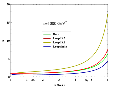
Figure 3: the ratios of $\mathrm{|M|^{2}_{Born}}$, $\mathrm{|M|^{2}_{Loop~{}IR2}}$, $\mathrm{|M|^{2}_{Loop~{}IR1}}$ and $\mathrm{|M|^{2}_{Loop~{}finite}}$ versus the quark mass in the process $\gamma^{*}+q\to Q\bar{Q}+q$.

From Fig.3 we can see that, for $s=1000~{}\mathrm{GeV^{2}}$ and $s=2000~{}\mathrm{GeV^{2}}$, the curves change little. As the quark mass gets larger, the NLO amplitude squared also gets larger quickly, even for the $\mathrm{|M|^{2}_{Loop~{}IR1}}$, the ratio is nearly $20$ when the quark mass is $6~{}\mathrm{GeV}$. So we may conclude that, in the $\gamma^{*}\longrightarrow Q\bar{Q}-Reggeon$ vertex, the quark mass effects on the photon impact factor are significant, and may influence the results of high energy photon-photon scattering and heavy quark pair leptoproduction.

VII Conclusions

In this paper, we calculated the process $\gamma^{*}+~{}q\longrightarrow Q\bar{Q}+q$ at NLO with fully virtual corrections in the high energy limit for massive quark pair $Q(\bar{Q}$, which tells the coupling of the reggeized gluon to $\gamma^{*}\longrightarrow Q\bar{Q}$. This calculation is just the first step of our final purpose, to obtain the complete NLO corrections to the photon impact factor and checking the BFKL pomeron prediction for the process $\gamma^{*}+\gamma^{*}\longrightarrow\gamma^{*}+\gamma^{*}$ at high energies.

In our calculation all contributions from loop diagrams, i.e., self-energy, triangle, box and pentagon diagrams, are regulated in dimensional regularization scheme and the ultraviolet divergences are renormalized by adding the corresponding counter terms. In the end, the infrared divergences still exist in the result, which would be canceled after taking account of the real corrections.

We find that for $\gamma^{*}+~{}q\longrightarrow Q\bar{Q}+q$ process in the massive quark case, the quark mass effects are significant at the next-to-leading order of accuracy, which indicates that for heavy quark diffractive photoproduction, the quark mass is indispensable. Our result might essentially show the quark mass effect, in spite of the absence of real corrections, which are needed in a complete NLO calculation. Moreover, for the photon impact factor with heavy quarks, the photon is legitimate to be real in order to guarantee the perturbative QCD calculations applicable.

Acknowledgments

This work was supported by the National Natural Science Foundation of China (NSFC) under grants 11905006, 11805042, 11975236 and 11635009.

Appendix

The loop integrals in LoopTools are defined as

$$C_{0}(p_{1}^{2},p_{2}^{2},p_{3}^{2},(p_{1}+p_{2})^{2},m_{1}^{2},m_{2}^{2},m_{3}^{2})=\frac{(2\pi\mu)^{4-2\epsilon}}{i\pi^{2}}\int\frac{d^{4-2\epsilon}q}{[q^{2}-m_{1}^{2}][(q+p_{1})^{2}-m_{2}^{2}][(q+p_{1}+p_{2})^{2}-m_{3}^{2}]},$$

$$D_{0}(p_{1}^{2},p_{2}^{2},(p_{1}+p_{2})^{2},(p_{2}+p_{3})^{2},m_{1}^{2},m_{2}^{2},m_{3}^{2},m_{4}^{2})$$

$$=\frac{(2\pi\mu)^{4-2\epsilon}}{i\pi^{2}}\int\frac{d^{4-2\epsilon}q}{[q^{2}-m_{1}^{2}][(q+p_{1})^{2}-m_{2}^{2}][(q+p_{1}+p_{2})^{2}-m_{3}^{2}][(q+p_{1}+p_{2}+p_{3})^{2}-m_{4}^{2}]},$$

$$\frac{(2\pi\mu)^{4-2\epsilon}}{i\pi^{2}}\int d^{4-2\epsilon}q\frac{q^{\mu}}{[q^{2}-m_{1}^{2}][(q+p_{1})^{2}-m_{2}^{2}][(q+p_{1}+p_{2})^{2}-m_{3}^{2}]}=\sum_{i=1}^{2}C_{i}p_{i}^{\mu},$$

$$\frac{(2\pi\mu)^{4-2\epsilon}}{i\pi^{2}}\int d^{4-2\epsilon}q\frac{q^{\mu}q^{\nu}}{[q^{2}-m_{1}^{2}][(q+p_{1})^{2}-m_{2}^{2}][(q+p_{1}+p_{2})^{2}-m_{3}^{2}]}=g^{\mu\nu}C_{00}+\sum_{i,j=1}^{2}C_{ij}p_{i}^{\mu}p_{j}^{\nu},$$

$$\frac{(2\pi\mu)^{4-2\epsilon}}{i\pi^{2}}\int d^{4-2\epsilon}q\frac{q^{\mu}}{[q^{2}-m_{1}^{2}][(q+p_{1})^{2}-m_{2}^{2}][(q+p_{1}+p_{2})^{2}-m_{3}^{2}][(q+p_{1}+p_{2}+p_{3})^{2}-m_{4}^{2}]}$$

$$=\sum_{i=1}^{3}D_{i}p_{i}^{\mu},$$

$$\frac{(2\pi\mu)^{4-2\epsilon}}{i\pi^{2}}\int d^{4-2\epsilon}q\frac{q^{\mu}q^{\nu}}{[q^{2}-m_{1}^{2}][(q+p_{1})^{2}-m_{2}^{2}][(q+p_{1}+p_{2})^{2}-m_{3}^{2}][(q+p_{1}+p_{2}+p_{3})^{2}-m_{4}^{2}]}$$

$$=g^{\mu\nu}D_{00}+\sum_{i,j=1}^{3}D_{ij}p_{i}^{\mu}p_{j}^{\nu},$$

$$\frac{(2\pi\mu)^{4-2\epsilon}}{i\pi^{2}}\int d^{4-2\epsilon}q\frac{q^{\mu}q^{\nu}q^{\rho}}{[q^{2}-m_{1}^{2}][(q+p_{1})^{2}-m_{2}^{2}][(q+p_{1}+p_{2})^{2}-m_{3}^{2}][(q+p_{1}+p_{2}+p_{3})^{2}-m_{4}^{2}]}$$

$$=\sum_{i=1}^{3}(g^{\mu\nu}p_{i}^{\rho}+g^{\nu\rho}p_{i}^{\mu}+g^{\mu\rho}p_{i}^{\nu})D_{00i}+\sum_{i,j,k=1}^{3}D_{ijk}p_{i}^{\mu}p_{j}^{\nu}p_{k}^{\rho}~{}.$$

All the coefficients such as $C_{ij}$, $D_{ijk}$ can be evaluated numerically by LoopTools.

In the following, we list the expressions that are not given in the main body of the paper:

$$A_{14}\, =\,\Gamma_{qq}^{(0),a}\frac{2s}{t}\bigg{(}\frac{ee_{f}}{s}\bigg{)}\bigg{(}\frac{N_{c}}{2}\bigg{)}\frac{1}{(4\pi)^{2}}\bigg{\{}H_{T}^{a}\big{[}3m^{2}D_{0}(14)+2(3m^{2}-t+t_{b})D_{1}(14)$$

$$+(2m^{2}+Q^{2}-2t+2t_{a}+4t_{b})D_{2}(14)-3Q^{2}D_{3}(14)+6D_{00}(14)+5m^{2}D_{11}(14)$$

$$+(4m^{2}+Q^{2}-5t+t_{a}+5t_{b})D_{12}(14)+4(m^{2}-Q^{2}-t_{a})D_{13}(14)$$

$$+(m^{2}+Q^{2}+4t_{b})D_{22}(14)-2(2m^{2}+Q^{2}-2t_{b})D_{23}(14)-3Q^{2}D_{33}(14)\big{]}$$

$$+mH_{p\varepsilon}^{a}\big{[}(3m^{2}+Q^{2}+2t_{a}-2t_{b})D_{0}(14)+(5m^{2}+2Q^{2}-2t+3t_{a})D_{1}(14)$$

$$+(3m^{2}+3Q^{2}-2t+4t_{a}+t_{b})D_{2}(14)-Q^{2}D_{3}(14)+6D_{00}(14)$$

$$+(4m^{2}+Q^{2}+t_{a})D_{11}(14)+(4m^{2}+3Q^{2}-5t+2t_{a}+4t_{b})D_{12}(14)$$

$$+2(2m^{2}-Q^{2}-2t_{a})D_{13}(14)+(2m^{2}+2Q^{2}+3t_{b})D_{22}(14)$$

$$+4(t_{b}-m^{2})D_{23}(14)-3Q^{2}D_{33}(14)\big{]}$$

$$+H_{p}^{a}\big{[}\varepsilon\cdot r\big{(}4m^{2}D_{1}(14)+2(Q^{2}-3m^{2}+2t_{a})D_{2}(14)-4Q^{2}D_{3}(14)+8D_{00}(14)$$

$$+4m^{2}D_{11}(14)-2(m^{2}-Q^{2}-t_{a})D_{12}(14)+4(m^{2}-Q^{2}-t_{a})D_{13}(14)$$

$$-2(m^{2}-Q^{2}-2t+t_{b})D_{22}(14)+4(t_{a}-m^{2})D_{23}(14)-4Q^{2}D_{33}(14)$$

$$-20D_{002}(14)-2(m^{2}-t+t_{b})D_{122}(14)+2(Q^{2}-m^{2}+t_{a})D_{123}(14)$$

$$-2t_{b}D_{222}(14)+2Q^{2}D_{233}(14)+2(m^{2}+Q^{2}-t_{b})D_{223}(14)\big{)}$$

$$+\varepsilon\cdot k\big{(}-6m^{2}D_{0}(14)-2(5m^{2}-2t+2t_{b})D_{1}(14)-2(5m^{2}-2t+2t_{b})D_{2}(14)$$

$$-2Q^{2}D_{3}(14)+4D_{00}(14)+(4t-6m^{2}-4t_{b})D_{11}(14)+4(t_{a}-t_{b})D_{13}(14)$$

$$-10(m^{2}-t+t_{b})D_{12}(14)-2(2m^{2}-2t+3t_{b})D_{22}(14)+4(t_{a}-t_{b})D_{23}(14)$$

$$-2Q^{2}D_{33}(14)-20D_{001}(14)-20D_{002}(14)-2(2m^{2}-t+t_{b})D_{112}(14)$$

$$+2(Q^{2}-m^{2}+t_{a})D_{113}(14)-2(m^{2}-t+2t_{b})D_{122}(14)+2Q^{2}D_{133}(14)$$

$$+2(2Q^{2}+t_{a}-t_{b})D_{123}(14)-2t_{b}D_{222}(14)+2(m^{2}+Q^{2}-t_{b})D_{233}(14)$$

$$+2Q^{2}D_{233}(14)\big{)}\big{]}+sH_{\varepsilon}^{a}\big{[}-2\alpha m^{2}D_{0}(14)+(m^{2}+Q^{2}-(7m^{2}+Q^{2})\alpha)D_{1}(14)$$

$$+((3-5\alpha)m^{2}+Q^{2}+2t-2t_{a}-2(Q^{2}+t_{b})\alpha)D_{2}(14)-2(1+2\alpha)D_{00}(14)$$

$$+(m^{2}+Q^{2}(1+2\alpha))D_{3}(14)-((1+3\alpha)m^{2}-(1-\alpha)(Q^{2}+t_{a}))D_{11}(14)$$

$$+((2-3\alpha)Q^{2}+t_{a}-t_{b}-\alpha(3m^{2}+2t_{a}+3t_{b})+2(\alpha+1)t)D_{12}(14)$$

$$+((Q^{2}+t_{a})(2\alpha+3)-(1+2\alpha)m^{2})D_{13}(14)$$

$$+(m^{2}+Q^{2}-t_{b}-2\alpha(m^{2}+Q^{2}+t_{b}))D_{22}(14)-2D_{003}(14)$$

$$+((3+2\alpha)m^{2}+3Q^{2}-(1+2\alpha)t_{b})D_{23}(14)+2(1+\alpha)Q^{2}D_{33}(14)$$

$$+2(\alpha-1)(D_{001}(14)+D_{002}(14))+(\alpha-1)(2m^{2}-t+t_{b})D_{112}(14)$$

$$+((\alpha-2)m^{2}+(1-\alpha)(Q^{2}+t_{a}))D_{113}(14)+(m^{2}-t+2t_{b})(\alpha-1)D_{122}(14)$$

$$+(-m^{2}+t+(\alpha-2)t_{b}-2Q^{2}(\alpha-1)+(1-\alpha)t_{a})D_{123}(14)$$

$$+(t_{a}-m^{2}+(2-\alpha)Q^{2})D_{133}(14)+(\alpha-1)t_{b}D_{222}(14)$$

$$+(m^{2}+Q^{2}-2t_{b}-\alpha(m^{2}+Q^{2}-t_{b}))D_{223}(14)$$

$$+(m^{2}-t_{b}-Q^{2}(\alpha-2))D_{233}(14)+Q^{2}D_{333}(14)\big{]}$$

$$+2mH_{m}^{a}\big{[}2s\big{(}(1+\alpha)D_{2}(14)+2D_{12}(14)+(3-\alpha))D_{22}(14)+(\alpha+2)D_{23}(14)$$

$$+(1-\alpha)D_{112}(14)+3(1-\alpha)D_{122}(14)+(2-\alpha)D_{123}(14)+2(1-\alpha)D_{222}(14)$$

$$+(3-\alpha)D_{223}(14)+2D_{233}(14)\big{)}\varepsilon\cdot r+2s\big{(}2\alpha D_{0}(14)+(1+3\alpha)D_{1}(14)+4\alpha D_{2}(14)$$

$$+2D_{11}(14)+4D_{12}(14)+(2+\alpha)D_{13}(14)+2D_{22}(14)+(1+\alpha)D_{23}(14)+D_{133}(14)$$

$$+(1-\alpha)D_{111}(14)+4(1-\alpha)D_{112}(14)+(2-\alpha)D_{113}(14)+5(1-\alpha)D_{122}(14)$$

$$+(5-2\alpha)D_{123}(14)+2(1-\alpha)D_{222}(14)+(3-\alpha)D_{223}(14)+D_{233}(14)\big{)}\varepsilon\cdot k$$

$$+\big{(}-(m^{2}+Q^{2}+2t_{a})D_{0}(14)-(2m^{2}+2Q^{2}+3t_{a})D_{1}(14)-(m^{2}+3Q^{2}-2t$$

$$+4t_{a}+t_{b})D_{2}(14)-(m^{2}+Q^{2})D_{3}(14)-6D_{00}(14)-(Q^{2}+t_{a})D_{11}(14)$$

$$-(3Q^{2}-t+2t_{a})D_{12}(14)-2Q^{2}D_{13}(14)+(t_{b}-2m^{2}-2Q^{2})D_{22}(14)$$

$$-4Q^{2}D_{23}(14)-Q^{2}D_{33}(14)+2D_{001}(14)+4D_{002}(14)+2D_{003}(14)+m^{2}D_{111}(14)$$

$$+(3m^{2}-t+t_{b})D_{112}(14)+(2m^{2}-Q^{2}-t_{a})D_{113}(14)+(2m^{2}-2t+3t_{b})D_{122}(14)$$

$$+(2m^{2}-3Q^{2}-t-2t_{a}+2t_{b})D_{123}(14)+(m^{2}-2Q^{2}-t_{a})D_{133}(14)+2t_{b}D_{222}(14)$$

$$+(3t_{b}-2m^{2}-2Q^{2})D_{223}(14)+(t_{b}-m^{2}-3Q^{2})D_{233}(14)-Q^{2}D_{333}(14)\big{)}\varepsilon\cdot p\big{]}$$

$$+2H_{k}^{a}\big{[}2s\big{(}(1-\alpha)D_{2}(14)+(1-\alpha)D_{12}(14)-\alpha D_{23}(14)+(\alpha-1)D_{122}(14)$$

$$+(\alpha-1)D_{123}(14)+(\alpha-1)D_{222}(14)+(\alpha-2)D_{223}(14)-D_{233}(14)\big{)}\varepsilon\cdot r$$

$$+2s\big{(}(1-\alpha)D_{2}(14)-(1+\alpha)D_{13}(14)-\alpha D_{23}(14)+(\alpha-1)D_{112}(14)$$

$$+(\alpha-1)D_{113}(14)+2(\alpha-1)D_{122}(14)+(2\alpha-3)D_{123}(14)-D_{133}(14)$$

$$+(\alpha-1)D_{222}(14)+(\alpha-2)D_{223}(14)-D_{233}(14)\big{)}\varepsilon\cdot k+\big{(}2m^{2}D_{0}(14)$$

$$+4m^{2}D_{1}(14)+(m^{2}+Q^{2}+2(t_{a}+t_{b}-t))D_{2}(14)+(m^{2}-Q^{2})D_{3}(14)$$

$$+2D_{00}(14)+(m^{2}+Q^{2}-2t+t_{a}+2t_{b})D_{12}(14)+(m^{2}-Q^{2}-t_{a})D_{13}(14)$$

$$+(m^{2}+Q^{2}+t_{b})D_{22}(14)+(Q^{2}-m^{2}+t_{b})D_{23}(14)-2D_{002}(14)-2D_{003}(14)$$

$$-m^{2}D_{112}(14)-m^{2}D_{113}(14)+(t-m^{2}-t_{b})D_{122}(14)+(Q^{2}-2m^{2}+t+t_{a}$$

$$-t_{b})D_{123}(14)+(Q^{2}-m^{2}+t_{a})D_{133}(14)-t_{b}D_{222}(14)+(m^{2}+Q^{2}-2t_{b})D_{223}(14)$$

$$+2m^{2}D_{11}(14)+(m^{2}+2Q^{2}-t_{b})D_{233}(14)+Q^{2}D_{333}(14)\big{)}\varepsilon\cdot p\big{]}$$

$$-4mH_{pk}^{a}\big{[}\big{(}2(D_{0}(14)+D_{11}(14)+D_{22}(14))+4(D_{1}(14)+D_{2}(14)+D_{12}(14))\big{)}\varepsilon\cdot k$$

$$+\big{(}D_{0}(14)+D_{1}(14)+3D_{2}(14)+2D_{12}(14)+2D_{22}(14)\big{)}\varepsilon\cdot r\big{]}$$

$$+2msH_{k\varepsilon}^{a}\big{(}(1-2\alpha)D_{0}(14)+(2-3\alpha)D_{1}(14)+(2-3\alpha)D_{2}(14)+(1-\alpha)D_{11}(14)$$

$$+2(1-\alpha)D_{12}(14)+(1-\alpha)D_{22}(14)+D_{13}(14)+D_{23}(14)\big{)}\bigg{\}}.$$ (53)

and $D_{i}(14)=D_{i}(m^{2},t,m^{2},-Q^{2},t_{b},t_{a},m^{2},0,0,m^{2})$.

$$A_{12}^{0}\, =\,-H_{T}^{a}\big{[}(3m^{2}D_{0}(12)_{fin}+(4m^{2}-M^{2})D_{1}(12)_{fin}+m^{2}D_{11}(12)_{fin})$$

$$+(2m^{2}+M^{2})(D_{2}(12)+D_{12}(12)+D_{22}(12)-D_{123}(12)-D_{223}(12))$$

$$-2D_{00}(12)+Q^{2}D_{33}(12)-6D_{003}(12)+Q^{2}D_{333}(12)$$

$$-(m^{2}-Q^{2}-t_{a})D_{133}(12)-(2m^{2}-2Q^{2}-t_{a}-t_{b})D_{233}(12)\big{]}$$

$$+mH_{p\varepsilon}^{a}\big{[}-(3m^{2}+t_{a}-t_{b})D_{0}(12)_{fin}-(4m^{2}+2Q^{2}-t+3t_{a})D_{1}(12)_{fin}$$

$$-(Q^{2}+t_{a})D_{11}(12)_{fin}+m^{2}D_{111}(12)_{fin}-(2m^{2}+M^{2})(D_{2}(12)+D_{22}(12)$$

$$-D_{112}(12)-D_{122}(12)-D_{223}(12))-(Q^{2}+t)D_{12}(12)-2Q^{2}D_{13}(12)$$

$$-Q^{2}D_{33}(12)+6D_{001}(12)+6D_{003}(12)+(2m^{2}-Q^{2}-t_{a})D_{113}(12)$$

$$+(4m^{2}-3Q^{2}+t-2t_{a}-2t_{b})D_{123}(12)+(m^{2}-2Q^{2}-t_{a})D_{133}(12)$$

$$+(2m^{2}-2Q^{2}-t_{a}-t_{b})D_{233}(12)-Q^{2}D_{333}(12)+2D_{00}(12)\big{]}$$

$$+sH_{\varepsilon}^{a}\big{[}\alpha m^{2}(D_{0}(12)_{fin}+3D_{1}(12)_{fin}+2D_{11}(12)_{fin})+2\alpha D_{00}(12)$$

$$+((1+\alpha)m^{2}+t-t_{a}-\alpha(2Q^{2}+t_{a}+t_{b}))D_{2}(12)-\alpha Q^{2}D_{3}(12)$$

$$+(4\alpha m^{2}+(1+\alpha)t-(1+2\alpha)t_{a}-2\alpha t_{b}-3\alpha Q^{2})D_{12}(12)$$

$$-(2\alpha Q^{2}-\alpha m^{2}+(1+\alpha)t_{a})D_{13}(12)+\alpha(2m^{2}-2Q^{2}-t_{a}-t_{b})D_{223}(12)$$

$$+((1+4\alpha)m^{2}+(1+\alpha)t-3\alpha Q^{2}-(1+2\alpha)t_{a}-2\alpha t_{b})D_{22}(12)$$

$$+((1+2\alpha)m^{2}-(1+\alpha)t_{a}-\alpha t_{b}-4\alpha Q^{2})D_{23}(12)-\alpha Q^{2}D_{233}(12)$$

$$-\alpha Q^{2}D_{33}(12)+2(\alpha-1)D_{001}(12)-2(1-3\alpha)D_{002}(12)-2D_{003}(12)$$

$$+\alpha(2m^{2}+M^{2})(D_{122}(12)+D_{222}(12))+\alpha(m^{2}-Q^{2}-t_{a})D_{123}(12)\big{]}$$

$$+sH_{k\varepsilon}^{a}\big{[}(2\alpha-1)D_{0}(12)_{fin}+(3\alpha-2)D_{1}(12)_{fin}$$

$$+(\alpha-1)D_{11}(12)_{fin}-D_{12}(12)-D_{13}(12)\big{]}$$

$$+2mH_{pk}^{a}\big{[}(2D_{0}(12)_{fin}+3D_{1}(12)_{fin}+D_{11}(12)_{fin})\varepsilon\cdot k$$

$$+(D_{0}(12)_{fin}+D_{1}(12)_{fin}-D_{12}(12))\varepsilon\cdot r\big{]}$$

$$+2sH_{k}^{a}\big{[}(D_{2}(12)+D_{12}(12)+(1+\alpha)D_{13}(12)+D_{22}(12)+D_{23}(12)$$

$$+(1-\alpha)D_{113}(12)+D_{123}(12)+D_{133}(12))\varepsilon\cdot k+((1-\alpha)(D_{2}(12)$$

$$+D_{12}(12)+D_{22}(12)-D_{123}(12))-\alpha D_{23}(12)-D_{223}(12)-D_{233}(12))\varepsilon\cdot r\big{]}$$

$$+2msH_{m}^{a}\big{[}(-2\alpha D_{0}(12)_{fin}-(1+3\alpha)D_{1}(12)_{fin}-2D_{11}(12)_{fin}+(\alpha-1)D_{111}(12)_{fin}$$

$$-D_{2}(12)-2D_{12}(12)-(\alpha+2)D_{13}(12)-D_{22}(12)-D_{23}(12)-D_{112}(12)$$

$$+(\alpha-2)D_{113}(12)-D_{123}(12))\varepsilon\cdot k+((1+\alpha)D_{2}(12)+2D_{12}(12)+(1+\alpha)D_{22}(12)$$

$$+(2+\alpha)D_{23}(12)+(1-\alpha)D_{112}(12)+(2-\alpha)D_{123}(12)+D_{122}(12)+D_{223}(12)$$

$$+D_{233}(12))\varepsilon\cdot r\big{]}$$

$$-2H_{p}^{a}\big{[}(-2m^{2}D_{0}(12)_{fin}-(2m^{2}-M^{2})D_{1}(12)_{fin}+(m^{2}+M^{2})D_{11}(12)_{fin}$$

$$-(m^{2}+Q^{2}+t)D_{2}(12)-(m^{2}+Q^{2})D_{3}(12)+(4m^{2}-3Q^{2}+t-2t_{a}-2t_{b})D_{12}(12)$$

$$+4D_{00}(12)+(2m^{2}-3Q^{2}-t_{a}-t_{b})D_{13}(12)+(2m^{2}-2Q^{2}-t_{a}-t_{b})D_{22}(22)$$

$$+(2m^{2}-4Q^{2}-t_{a}-t_{b})D_{23}(12)-2Q^{2}D_{33}(12)+6D_{002}(12)+6D_{003}(12)$$

$$+(3m^{2}+M^{2})D_{112}(12)+(2m^{2}-Q^{2}-t_{a})D_{113}(12)+2(2m^{2}+M^{2})D_{122}(12)$$

$$+(5m^{2}-4Q^{2}+t-3t_{a}-2t_{b})D_{123}(12)+m^{2}D_{111}(12)_{fin}+(2m^{2}+M^{2})D_{222}(12)$$

$$+(m^{2}-2Q^{2}-t_{a})D_{133}(12)+(4m^{2}-3Q^{2}+t-2t_{a}-2t_{b})D_{223}(12)+4D_{001}(12)$$

$$+(2m^{2}-3Q^{2}-t_{a}-t_{b})D_{233}(12)-Q^{2}D_{333}(12))\varepsilon\cdot k+(m^{2}D_{1}(12)_{fin}+m^{2}D_{11}(12)_{fin}$$

$$+(Q^{2}-m^{2}+t_{a})D_{2}(12)-Q^{2}D_{3}(12)+2D_{00}(12)-Q^{2}D_{33}(12)+2D_{002}(12)$$

$$+(m^{2}-Q^{2}-t_{a})(D_{13}(12)+D_{22}(12))+(m^{2}-2Q^{2}-t_{a})D_{23}(12))\varepsilon\cdot r\big{]}$$

$$+2\varepsilon\cdot pH_{k}^{a}\big{[}-m^{2}D_{0}(12)_{fin}-2m^{2}D_{1}(12)_{fin}-m^{2}D_{11}(12)_{fin}-(2m^{2}+M^{2})\times$$

$$(D_{2}(12)+D_{12}(12)+D_{22}(12)-D_{123}(12)-D_{223}(12))-m^{2}D_{3}(12)-Q^{2}D_{33}(12)$$

$$+4D_{003}(12)+m^{2}D_{113}(12)+(2m^{2}-2Q^{2}-t_{a}-t_{b})D_{233}(12)-Q^{2}D_{333}(12)$$

$$+(m^{2}-Q^{2}-t_{a})D_{133}(12)\big{]}$$

$$+2mH_{m}^{a}\varepsilon\cdot p\big{[}(m^{2}+Q^{2}+t_{a})D_{0}(12)_{fin}+(m^{2}+2Q^{2}+2t_{a})D_{1}(12)_{fin}$$

$$+(Q^{2}-m^{2}+t_{a})D_{11}(12)_{fin}-m^{2}D_{111}(12)_{fin}+(Q^{2}+t)D_{2}(12)$$

$$+(m^{2}+2Q^{2})D_{3}(12)+(2Q^{2}-2m^{2}+t_{a}+t_{b})D_{12}(12)+2Q^{2}D_{33}(12)$$

$$-(m^{2}-3Q^{2}-t_{a})D_{13}(12)-(2m^{2}-2Q^{2}-t_{a}-t_{b})D_{23}(12)-4D_{001}(12)$$

$$-(2m^{2}+M^{2})(D_{112}(12)+D_{122}(12)+D_{223}(12))+(Q^{2}-2m^{2}+t_{a})D_{113}(12)$$

$$-(4m^{2}-3Q^{2}+t-2t_{a}-2t_{b})D_{123}(12)-(m^{2}-2Q^{2}-t_{a})D_{133}(12)$$

$$-4D_{003}(12)+(2Q^{2}-2m^{2}+t_{a}+t_{b})D_{233}(12)+Q^{2}D_{333}(12)\big{]}.$$ (54)

here $D_{i}(12)=D_{i}(m^{2},m^{2},t,-Q^{2},2m^{2}+M^{2},t_{a},m^{2},0,m^{2},m^{2})$.

$$\bar{A}_{12}^{0}\, =\,-H_{T}^{a}\big{[}(3m^{2}D_{0}(\bar{12})_{fin}+(4m^{2}-M^{2})D_{1}(\bar{12})_{fin}+m^{2}D_{11}(\bar{12})_{fin})$$

$$+(2m^{2}+M^{2})(D_{2}(\bar{12})+D_{12}(\bar{12})+D_{22}(\bar{12})-D_{123}(\bar{12})-D_{223}(\bar{12}))$$

$$-2D_{00}(\bar{12})+Q^{2}D_{33}(\bar{12})-6D_{003}(\bar{12})-(m^{2}-Q^{2}-t_{b})D_{133}(\bar{12})$$

$$-(2m^{2}-2Q^{2}-t_{b}-t_{a})D_{233}(\bar{12})+Q^{2}D_{333}(\bar{12})\big{]}$$

$$-mH_{p\varepsilon}^{a}\big{[}(3m^{2}+t_{a}-t_{b})D_{0}(\bar{12})_{fin}+(4m^{2}-t+2t_{a}-t_{b})D_{1}(\bar{12})_{fin}$$

$$+(2m^{2}-Q^{2}-t_{b})D_{11}(\bar{12})_{fin}+m^{2}D_{111}(\bar{12})_{fin}+m^{2}D_{3}(\bar{12})$$

$$+(2m^{2}+M^{2})(D_{2}(12)+D_{22}(12)+D_{112}(\bar{12})+D_{122}(\bar{12})-D_{223}(\bar{12}))$$

$$+(4m^{2}-3Q^{2}+t-2t_{a}-2t_{b})D_{12}(\bar{12})-2Q^{2}D_{13}(\bar{12})+Q^{2}D_{33}(\bar{12})$$

$$+6D_{001}(\bar{12})-6D_{003}(\bar{12})-(Q^{2}+t_{b})D_{113}(\bar{12})-(Q^{2}+t)D_{123}(\bar{12})$$

$$+(m^{2}-t_{b})D_{133}(\bar{12})-(2m^{2}-2Q^{2}-t_{a}-t_{b})D_{233}(\bar{12})+Q^{2}D_{333}(\bar{12})\big{]}$$

$$+sH_{\varepsilon}^{a}\big{[}(\alpha+2)m^{2}D_{0}(\bar{12})_{fin}+((3\alpha+1)m^{2}-M^{2})D_{1}(\bar{12})_{fin}$$

$$+(2\alpha-1)m^{2}D_{11}(\bar{12})_{fin}+(\alpha m^{2}+(1-2\alpha)Q^{2}-\alpha t_{a}+(1-\alpha)t_{b})D_{2}(\bar{12})$$

$$+(m^{2}+(1-\alpha)Q^{2})D_{3}(\bar{12})+2(\alpha-2)D_{00}(\bar{12})$$

$$+(2(2\alpha-1)m^{2}+(2-3\alpha)Q^{2}+(\alpha-1)(t+2t_{b})+(1-2\alpha)t_{a})D_{12}(\bar{12})$$

$$+(2(1-\alpha)Q^{2}+(\alpha-1)m^{2}+(2-\alpha)t_{b})D_{13}(\bar{12})$$

$$+((4\alpha-3)m^{2}+(\alpha-1)t+(2-3\alpha)Q^{2}+(1-2\alpha)t_{a}+2(1-\alpha)t_{b})D_{22}(\bar{12})$$

$$+((2\alpha-3)m^{2}+(1-\alpha)t_{a}+(2-\alpha)t_{b}-4(1-\alpha)Q^{2})D_{23}(\bar{12})$$

$$+(2-\alpha)Q^{2}D_{33}(\bar{12})+2\alpha D_{001}(\bar{12})+2(3\alpha-2)D_{002}(\bar{12})-4D_{003}(\bar{12})$$

$$+(\alpha-1)(2m^{2}+M^{2})(D_{122}(\bar{12})+D_{222}(\bar{12}))+(Q^{2}-m^{2}+t_{b})D_{133}(\bar{12})$$

$$+(2(\alpha-2)m^{2}+(3-2\alpha)Q^{2}-t+(2-\alpha)(t_{a}+t_{b}))D_{223}(\bar{12})$$

$$+((\alpha-3)m^{2}+(2-\alpha)Q^{2}-t+t_{a}+(2-\alpha)t_{b})D_{123}(\bar{12})+(\alpha-1)m^{2}D_{112}(\bar{12})$$

$$+((3-\alpha)Q^{2}-2m^{2}+t_{a}+t_{b})D_{233}(\bar{12})+Q^{2}D_{333}(\bar{12})-m^{2}D_{113}(\bar{12})\big{]}$$

$$+sH_{k\varepsilon}^{a}\big{[}(2\alpha-1)D_{0}(\bar{12})_{fin}+(3\alpha-1)D_{1}(\bar{12})_{fin}+\alpha D_{11}(\bar{12})_{fin}+D_{12}(\bar{12})$$

$$+D_{13}(\bar{12})\big{]}+2mH_{pk}^{a}\big{[}(2D_{0}(\bar{12})_{fin}+3D_{1}(\bar{12})_{fin}+D_{11}(\bar{12})_{fin})\varepsilon\cdot k$$

$$+(D_{0}(\bar{12})_{fin}+2D_{1}(\bar{12})_{fin}+D_{11}(\bar{12})_{fin}+D_{12}(\bar{12}))\varepsilon\cdot r\big{]}$$

$$+2sH_{k}^{a}\big{[}(D_{2}(\bar{12})+D_{12}(\bar{12})+(2-\alpha)D_{13}(\bar{12})+D_{22}(\bar{12})$$

$$+D_{23}(\bar{12})+\alpha D_{113}(\bar{12})+D_{123}(\bar{12})+D_{133}(\bar{12}))\varepsilon\cdot k$$

$$+((1-\alpha)(D_{2}(\bar{12})+D_{12}(\bar{12})+D_{22}(\bar{12}))+\alpha D_{113}(\bar{12})+D_{133}(\bar{12})$$

$$+(2-\alpha)(D_{13}(\bar{12})+D_{23}(\bar{12}))+(1+\alpha)D_{123}(\bar{12})+D_{223}(\bar{12})+D_{233}(\bar{12}))\varepsilon\cdot r\big{]}$$

$$+2msH_{m}^{a}\big{[}(-2\alpha D_{0}(\bar{12})_{fin}+(1-3\alpha)D_{1}(\bar{12})_{fin}+D_{11}(\bar{12})_{fin}+\alpha D_{111}(\bar{12})_{fin}$$

$$-D_{2}(\bar{12})-(1-\alpha)D_{13}(\bar{12})-D_{22}(\bar{12})-D_{23}(\bar{12})+D_{112}(\bar{12})+(1-\alpha)D_{113}(\bar{12})$$

$$-D_{123}(\bar{12})-D_{133}(\bar{12}))\varepsilon\cdot k+(D_{1}(\bar{12})_{fin}+(1+\alpha)D_{11}(\bar{12})_{fin}+\alpha D_{111}(\bar{12})_{fin}$$

$$-D_{2}(\bar{12})+(1+\alpha)(2D_{12}(\bar{12})+D_{22}(\bar{12})+D_{112}(\bar{12}))+(1-\alpha)D_{113}(\bar{12})$$

$$+\alpha D_{23}(\bar{12})-\alpha D_{123}(\bar{12})+D_{122}(\bar{12})-D_{133}(\bar{12})-D_{223}(\bar{12})-D_{233}(\bar{12}))\varepsilon\cdot r\big{]}$$

$$-2H_{p}^{a}\big{[}(-2m^{2}D_{0}(\bar{12})_{fin}-(2m^{2}-M^{2})D_{1}(\bar{12})_{fin}+(m^{2}+M^{2})D_{11}(\bar{12})_{fin}$$

$$+m^{2}D_{111}(\bar{12})_{fin}-(m^{2}+Q^{2}+t)D_{2}(\bar{12})-(m^{2}+Q^{2})D_{3}(\bar{12})+4D_{00}(\bar{12})$$

$$+(4m^{2}-3Q^{2}+t-2t_{a}-2t_{b})D_{12}(\bar{12})+(2m^{2}-3Q^{2}-t_{a}-t_{b})D_{13}(\bar{12})$$

$$+4D_{001}(\bar{12})+(2m^{2}-2Q^{2}-t_{a}-t_{b})D_{22}(\bar{12})+6D_{002}(\bar{12})+6D_{003}(\bar{12})$$

$$+(2m^{2}-4Q^{2}-t_{a}-t_{b})D_{23}(\bar{12})-2Q^{2}D_{33}(\bar{12})+(3m^{2}+M^{2})D_{112}(\bar{12})$$

$$+(2m^{2}-Q^{2}-t_{b})D_{113}(\bar{12})+(5m^{2}-4Q^{2}+t-2t_{a}-3t_{b})D_{123}(\bar{12})$$

$$+(m^{2}-2Q^{2}-t_{b})D_{133}(\bar{12})+(4m^{2}-3Q^{2}+t-2t_{a}-2t_{b})D_{223}(\bar{12})$$

$$+2(2m^{2}+M^{2})D_{122}(\bar{12})+(2m^{2}+M^{2})D_{222}(\bar{12})-Q^{2}D_{333}(\bar{12})$$

$$+(2m^{2}-3Q^{2}-t_{a}-t_{b})D_{233}(\bar{12}))\varepsilon\cdot k$$

$$+(m^{2}D_{0}(\bar{12})_{fin}+m^{2}D_{1}(\bar{12})_{fin}+m^{2}D_{11}(\bar{12})_{fin}+m^{2}D_{111}(\bar{12})_{fin}$$

$$-(Q^{2}+t_{a})D_{2}(\bar{12})+(4m^{2}-3Q^{2}+2t-3t_{a}-2t_{b})D_{12}(\bar{12})$$

$$+(m^{2}-2Q^{2}-t_{a})D_{13}(\bar{12})+(3m^{2}-2Q^{2}+t-2t_{a}-t_{b})D_{22}(\bar{12})$$

$$+(m^{2}-2Q^{2}-t_{a})D_{23}(\bar{12})+4D_{001}(\bar{12})+(3m^{2}+M^{2})D_{112}(\bar{12})$$

$$+4D_{002}(\bar{12})+(m^{2}-Q^{2}-t_{b})D_{113}(\bar{12})+2(2m^{2}+M^{2})D_{122}(\bar{12})$$

$$+(3m^{2}-3Q^{2}-t_{a}-2t_{b})D_{123}(\bar{12})+(2m^{2}+M^{2})D_{222}(\bar{12})$$

$$+(2m^{2}-2Q^{2}-t_{a}-t_{b})D_{223}(\bar{12})-Q^{2}D_{133}(\bar{12})-Q^{2}D_{233}(\bar{12}))\varepsilon\cdot r\big{]}$$

$$+2\varepsilon\cdot pH_{k}^{a}\big{[}-2m^{2}D_{0}(\bar{12})_{fin}-(2m^{2}-M^{2})D_{1}(\bar{12})_{fin}+2D_{00}(\bar{12})_{fin}+2D_{003}(\bar{12})_{fin}\big{]}$$

$$+2mH_{m}^{a}\varepsilon\cdot p\big{[}(2m^{2}+Q^{2}+t_{a})D_{0}(\bar{12})_{fin}+(m^{2}+2Q^{2}-t+2t_{a}+t_{b})D_{1}(\bar{12})_{fin}$$

$$-m^{2}D_{11}(\bar{12})_{fin}-(2m^{2}-2Q^{2}-t_{a}-t_{b})D_{2}(\bar{12})+2Q^{2}D_{3}(\bar{12})-2D_{00}(\bar{12})$$

$$+(Q^{2}-2m^{2}-t+t_{a}+t_{b})D_{12}(\bar{12})-(2m^{2}-2Q^{2}-t_{a}-t_{b})D_{23}(\bar{12})$$

$$+(Q^{2}-m^{2}+t_{b})D_{13}(\bar{12})+Q^{2}D_{33}(\bar{12})+2D_{001}(\bar{12})-2D_{003}(\bar{12})\big{]}.$$ (55)

here $D_{i}(\bar{12})=D_{i}(m^{2},m^{2},-Q^{2},t,2m^{2}+M^{2},t_{b},m^{2},0,m^{2},m^{2})$.

$$A_{13}^{(0)}\, =\,H_{T}^{a}\big{\{}\alpha(\alpha-1)t(t_{a}-t_{b})[(\alpha-1)sD_{0}(2)-\alpha sD_{0}(1)]$$

$$-(\alpha-1)(2\Delta+(\alpha-1)\alpha(t_{a}-t_{b})(t_{a}-m^{2}))sD_{0}(3)$$

$$-\alpha(2\Delta+(\alpha-1)\alpha(t_{b}-t_{a})(t_{b}-m^{2}))sD_{0}(4)$$

$$-[2(\alpha-1)\alpha m^{6}+m^{4}(2(\alpha^{2}-\alpha-1)t-3(\alpha-1)\alpha(t_{a}+t_{b}))$$

$$+m^{2}(2t(\alpha(\alpha-1)Q^{2}-\alpha(\alpha-2)t_{a}+(1-\alpha^{2})t_{b})-2t^{2}$$

$$+(\alpha-1)\alpha(t_{a}^{2}+4t_{a}t_{b}+t_{b}^{2}))+(\alpha-1)\alpha(2t-t_{a}-t_{b})(Q^{2}t+t_{a}t_{b})]D_{0}(14)\big{\}}$$

$$+(sH_{\varepsilon}^{a}-2(H_{k}^{a}-mH_{m})\varepsilon\cdot p)\big{\{}t(\alpha-1)\alpha(t_{a}-m^{2})(\alpha sD_{0}(1)-(\alpha-1)sD_{0}(2))$$

$$-\alpha(-\Delta+m^{2}t-(\alpha-1)\alpha Q^{2}t)sD_{0}(4)+(\alpha-1)^{2}\alpha(t_{a}-m^{2})^{2}sD_{0}(3)$$

$$-[-(\alpha-1)\alpha m^{6}+\alpha m^{4}((\alpha-1)(2t_{a}+t_{b})-2(\alpha-2)t)$$

$$+m^{2}(\alpha t(-(\alpha-1)Q^{2}+2\alpha(t_{a}+t_{b})-2(2t_{a}+t_{b}))+2t^{2}-(\alpha-1)\alpha t_{a}(t_{a}+2t_{b}))$$

$$-(\alpha-1)\alpha(2t-t_{a})(Q^{2}t+t_{a}t_{b})]D_{0}(14)\big{\}}$$

$$+2t\Delta(H_{T}^{a}+mH_{p\varepsilon}^{a}-sH_{\varepsilon}^{a}-2H_{p}^{a}\varepsilon\cdot k+2(H_{k}^{a}-mH_{m}^{a})\varepsilon\cdot p)D_{0}(14)$$

$$+mH_{p\varepsilon}^{a}\big{\{}t(t-(\alpha-1)\alpha(t_{a}-t_{b}))(\alpha sD_{0}(1)-(\alpha-1)sD_{0}(2))$$

$$-[2(\alpha-1)\alpha m^{4}-m^{2}(3t+(\alpha-1)\alpha(t_{a}+3t_{b}))$$

$$+t(2(\alpha-1)\alpha Q^{2}+t_{b})+(\alpha-1)\alpha t_{b}(t_{a}+t_{b})]\alpha sD_{0}(4)$$

$$-[2(\alpha-1)\alpha m^{4}-m^{2}(t+(\alpha-1)\alpha(t_{b}+3t_{a}))$$

$$+t(2(\alpha-1)\alpha Q^{2}-t_{a})+(\alpha-1)\alpha t_{a}(t_{a}+t_{b})](\alpha-1)sD_{0}(3)$$

$$-[2(\alpha-1)\alpha m^{6}+m^{4}(t(2\alpha^{2}-4\alpha-1)-3(\alpha-1)\alpha(t_{a}+t_{b}))$$

$$+m^{2}(t(-2\alpha^{2}(t_{a}+t_{b}-Q^{2})+2\alpha(3t_{a}+t_{b}-Q^{2})-t_{a}+t_{b})$$

$$-2t^{2}+(\alpha-1)\alpha(t_{a}^{2}+4t_{a}t_{b}+t_{b}^{2}))$$

$$+(Q^{2}t+t_{a}t_{b})((2\alpha^{2}-4\alpha+1)t-(\alpha-1)\alpha(t_{a}+t_{b}))]D_{0}(14)\big{\}}$$

$$+2mtH_{pk}^{a}\varepsilon\cdot p\big{\{}-\alpha tD_{0}(1)+(\alpha-1)tD_{0}(2)$$

$$+\alpha(t_{b}-m^{2})D_{0}(4)-(\alpha-1)(t_{a}-m^{2})D_{0}(3)$$

$$+(1-2\alpha)(m^{4}-m^{2}(t_{a}+t_{b})+Q^{2}t+t_{a}t_{b})D_{0}(14)/s\big{\}}$$

$$+2H_{p}^{a}\big{\{}t(\alpha(\alpha-1)s(m^{2}-t_{a})\varepsilon\cdot r-tm^{2}\varepsilon\cdot p)\alpha D_{0}(1)$$

$$+t(\alpha(\alpha-1)s(t_{a}-m^{2})\varepsilon\cdot r+tm^{2}\varepsilon\cdot p)(\alpha-1)D_{0}(2)$$

$$+(t_{a}-m^{2})(\alpha(\alpha-1)s(m^{2}-t_{a})\varepsilon\cdot r-tm^{2}\varepsilon\cdot p)(\alpha-1)D_{0}(3)$$

$$-(s(\Delta-m^{2}t+(\alpha-1)\alpha Q^{2}t)\varepsilon\cdot r+m^{2}t(m^{2}-t_{b})\varepsilon\cdot p)\alpha D_{0}(4)$$

$$-[(2\alpha-1)m^{2}t(m^{4}-m^{2}(t_{a}+t_{b})+Q^{2}t+t_{a}t_{b})\varepsilon\cdot p/s$$

$$+(m^{2}-t_{a})(\Delta+m^{2}t(1-2\alpha))\varepsilon\cdot r-2t\Delta\varepsilon\cdot k]D_{0}(14)$$

$$-2t\Delta\varepsilon\cdot k(D_{1}(14)+D_{2}(14))-2t\Delta\varepsilon\cdot rD_{2}(14)\big{\}}.$$ (56)

and

$$D_{0}(1) = D_{0}(m^{2},0,0,t_{a},\alpha s,t,m^{2},0,0,0)_{fin}$$

$$D_{0}(2) = D_{0}(m^{2},0,0,t_{b},(\alpha-1)s,t,m^{2},0,0,0)_{fin}$$

$$D_{0}(3) = D_{0}(m^{2},0,\alpha s,-Q^{2},(\alpha-1)s,t_{a},m^{2},0,0,m^{2})_{fin}$$

$$D_{0}(4) = D_{0}(m^{2},0,(\alpha-1)s,-Q^{2},\alpha s,t_{b},m^{2},0,0,m^{2})_{fin}.$$ (57)

$D_{i}(14)$ is defined in the above paragraphs. The finite parts of these four-point integrals can also be obtained from ellis , or evaluated by LoopTools numerically.

References

- (1) E. Levin, hep-ph/9808486.
- (2) P. V. Landshoff, hep-ph/0108156.
- (3) V. A. Petrov, and A. V. Prokudin, Eur. Phys. J. C 23 (2002) 135 .
- (4) V. S. Fadin, R. Fiore and A. Quartarolo, Phys. Rev. D50 (1994) 2265.
- (5) V. S. Fadin, D. Ivanov, and M. Kotsky, hep-ph/0007119.
- (6) F. Yuan and K. T. Chao, Phys. Rev. D60 (1999) 094012.
- (7) F. Yuan and K. T. Chao, Phys. Rev. D58 (1998) 114016.
- (8) V. S. Fadin, and L. N. Lipatov, Phys. Lett. B 429 (1998) 127.
- (9) J. Bartels, A. De Roeck, H. Lotter, Phys. Lett. B 389 (1996) 742.
- (10) S. J. Brodsky, F. Hautmann, and D. E. Soper, Phys. Rev. D56 (1997) 6957; Phys. Rev. Lett. 78 (1997) 803 .
- (11) CEPC design performance considerations, arXiv:1501.06854.
- (12) ILC, Basic Conceptual Design Report, http://www.linearcollider.org.
- (13) EIC, Basic Conceptual Design Report, arXiv:1212.1701.
- (14) D. P. Anderle . Frontiers of Physics 64701 (2021) 16 Issue (6).
- (15) J. Bartels, C. Ewerz, and R. Staritzbichler, Phys. Lett. B 492 (2000) 56.
- (16) A. Donnachie, S. Sldner-Rembold, J. Phys. G 26 (2000) 689.
- (17) S. J. Brodsky, V. S. Fadin, V. T. Kim, L. N. Lipatov, and G. B. Pivovarov, JETP Lett. 70 (1999) 155.
- (18) M. Ciafaloni, G. Camici, Phys. Lett. B 430 (1998) 349.
- (19) S. Gieseke, Nucl. Phys. B 121 (2003) 42.
- (20) J. Bartels, D. Colferai, S. Gieseke and A. Kyrieleis, Phys. Rev. D66 (2002) 094017.
- (21) J. Bartels, Nucl. Phys. B 116 (2003) 126.
- (22) J. Bartels, S. Gieseke and C. F. Qiao, Phys. Rev. D63 (2001) 056014 [Erratum-ibid. D65 (2002) 079902].
- (23) T.Hahn, Comput. Phys. Commun. 140 (2001) 418 .
- (24) R.Metig, M.Bhm and A.Denner, Comput. Phys. Commun. 64 (1991) 345 .
- (25) T.Haln and M.Prez-Victoria, Comput. Phys. Commun. 118 (1999) 153
- (26) A.Denner and S.Dittmaier, Nucl. Phys. B 658 (2003) 175 .
- (27) R.Keith Ellis, Giulia Zanderighi, JHEP 0802 (2008) 002.