Performance of the GPU inverters with Chroma+QUDA for various fermion actions

Abstract

We present our progress on the Chroma interfaces of the twisted-mass, HISQ (highly improved staggered quark) and overlap fermion inverters using QUDA.

1 Introduction

When we put the fermion on the lattice, it is unavoidable to replace the derivative by the difference of the forward and backward shifts, and introduce the fermion doubling problem. There are various kinds of the discretized fermion action to solve or avoid the doubling problem: The simplest solution is the Wilson action which adds a second order derivative term (Wilson term); and the clover action add one more term to suppress the additional chiral symmetry breaking (A$\chi$SB) introduced by the Wilson term. The twisted-mass action multiplies a complex phase on the quark mass term of the Wilson action to achieve a better suppression on A$\chi$SB comparing to the clover action case, while adding a clover term is still beneficial to suppress the residual discretization errors. On the other hand, the staggered action maps the Dirac spinors to the lattice sites to weaken the doubling problem, while introduces the taste degree of freedom which makes the data analysis to be highly non-trivial. Finally, the overlap action (and the domain wall action as its approximation) can be considered as ultimate solution to avoid A$\chi$SB, while it can be much more expensive than the other actions.

Even though all kinds of the actions should approach the same continuum limit, their discretization error can be quite different. Thus it is essential to compare the results with different action at several lattice spacings, and have a trade-off between the statistical uncertainty and the systematic ones. But most of the Lattice QCD software concentrates on one or two fermion actions only, and then it can be quite non-trivial to switch the actions in the production and/or compare the corresponding results. Thus it is very helpful if one can calculate fermion propagators for all the actions in a given software, like Chroma.

The Chroma [4] package is an open-source Lattice QCD software at the level 4 of the USQCD SciDAC modules, and targets an uniform interface of the various algorithms like the fermion and gauge actions, solvers, and even monomial in HMC. At the same time, the QUDA [7, 8, 5] package provides the GPU-accelerated inverter for most of the fermion action except the overlap action (but most of the needed linear algebra operations are ready). Thus the missing pieces are just a Chroma interface to call kinds of the QUDA inverter, and also an implementation of the overlap action.

Tag	$6/g^{2}$	$L$	$T$	$a(\mathrm{fm})$	$m^{\textrm{w}}_{q}a$	$c_{\mathrm{sw}}$
MILC12	3.60	24	64	0.1213(9)	-0.0695	1.0509
MILC09	3.78	32	96	0.0882(7)	-0.0514	1.0424
MILC06	4.03	48	144	0.0574(5)	-0.0398	1.0349

tag	$6/g^{2}$	$L$	$T$	$a(\mathrm{fm})$	$m^{\textrm{ov}}_{q}a$
RBC11	2.13	24	64	0.1105(3)	0.015
RBC08	2.25	32	64	0.0828(3)	0.011

Table 1: Informations of the MILC and RBC ensembles used in this work.

2 Numerical setup and results

In this proceeding, we present the performance of GPU-accelerated inverter based on QUDA for three actions: Twisted-mass, HISQ and also overlap. The information of the gauge ensembles we used are summarized in Table 1. The node we used in this work include 32 CPU cores at 2 GHz and 4 V100 GPUs.

2.1 Twisted-mass fermion

The twisted-mass fermion action is defined as the following

$$S^{\rm tw}=\sum_{x,y}\bar{\psi}(x)D_{W}(x,y;m_{\rm cri}+\omega)\psi(x),$$ (1)

where

$$D_{w}(x,y;m)=\frac{1}{2}\sum_{\mu=1,...,4,\eta=\pm}(1+\eta\gamma_{\mu})U_{\mu}(x,x+\eta\hat{n}_{\mu}a)\delta_{y,x+\eta\hat{n}_{\mu}a}-(4+m)\delta_{x,y}$$ (2)

is the discretized $\not{D}$ of the Wilson action, $m_{\rm cri}$ is the quark mass parameter to make the corresponding pion mass to be zero, and $\omega$ is a complex number and corresponds to the degenerated twisted-mass parameters. The standard Wilson action corresponds to the case with a real value of $\omega$, and a purely imaginary $\omega$ will have an automatic ${\cal O}(a)$ improvement and avoid the exceptional condition due to the instability of the critical point. One can also add a clover term on the above action to get twisted-mass clover fermion action,

$$S^{\rm twc}=S^{\rm tw}+c^{\rm sw}\sigma_{\mu\nu}F^{\mu\nu}$$ (3)

which can further suppress the ${\cal O}(a^{2})$ discretization errors.

Tag	Ensembles	$m_{\rm cri}+\omega$	Nodes	Invertion	Setup
CPU with BICGSTAB	MILC06	-0.0398	9	6992s	-
GPU with GCR	MILC06	-0.0398	9	652s	-
GPU with multigrid	MILC06	-0.0398	9	99s	515s
GPU with multigrid	MILC06	-0.044+0.005i	9	78s	154s

Table 2: The inverstion and setup time needed by a 12-column propagator in different cases with a similar residual $10^{-6}$.

The QUDA interface of the twisted-mass action is quite similar to that of the clover one. The only subtle issue is that the inverse of the clover term has a complex diagonal part and then can not be packed for QUDA normally. Thus one would like to enable the dynamical-clover flag in QUDA, and calculate the entire clover term (and its inverse) in QUDA directly.

The comparison of the time needed by a full propagator with 12 columns are summarized in Table 2. Both the pion mass in the Clover and Twisted+clover cases are tuned to be about 300 MeV. One can see that the standard GPU inverter with GCR algorithm is around 10 times further than the CPU one with BICGSTAB algorithm, and the multi-grid inverter can be even faster, with the cost of the reusable subspace setup. Comparing the clover fermion action, the time need by the twisted-mass action is shorter with similar multi-grid parameters, especially during the setup.

2.2 HISQ fermion

Another solution of the fermion doubling problem is the staggered fermion. With a redefinition on the fermion field, we can obtain the staggered fermion action as the following,

$$S^{\rm st}=\sum_{x}\bar{\psi}^{\rm st}(x)\big{[}\frac{1}{2}\sum_{\mu=1,...,4,\eta=\pm}\eta\gamma_{\mu}U_{\mu}(x,x+\eta\hat{n}_{\mu}a)\psi(x+\eta\hat{n}_{\mu}a)-m\big{]}\psi^{\rm st}(x)$$ (4)

where $\psi^{\rm st}(x)=\gamma_{4}^{x_{4}}\gamma_{1}^{x_{1}}\gamma_{2}^{x_{2}}\gamma_{3}^{x_{3}}\psi(x)$ at the site $x=\{x_{1},x_{2},x_{3},x_{4}\}$ in the MILC conversion. Note that there is still 4 degrees of freedom which called taste, and the data analsysis with the taste mixing can be much more complicated. The HISQ action is an improved staggered action which include both the 1-step fat link (with certain smearing) and also 3-step long link [3].

One should be careful to compare the propagagor from the QUDA with that from the native Chroma HISQ inverter, since the Chroma HISQ action uses the CPS conversion $\psi^{\rm cps}(x)=\gamma_{1}^{x_{1}}\gamma_{2}^{x_{2}}\gamma_{3}^{x_{3}}\gamma_{4}^{x_{4}}\psi(x)$, and has different sign on the mass term. Thus effectively two conversions can be related with the following relation: $\psi^{\rm Chroma}(x)=(-1)^{(t\%2)((x+y+z)\%2)+(x+y+z+t)\%2}\psi^{\rm QUDA}$.

Similarly, we can see significant speed up of the GPU inverter comparing to the CPU one, especially when we use fewer nodes to do the test on small lattices. For multigrid, we apply KD Preconditioning [11].

The multigrid inverter requires very long time to generate the subspace, and the inverter is not faster than the standard CG algrithm even after the subspace is generated. The parameters we use are shown in Fig.1.

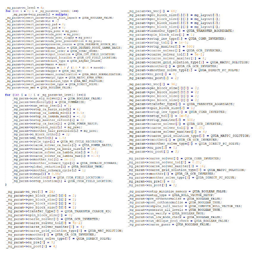
Figure 1: The parameters for HISQ multigrid, most of which are copied from MILC interface.

tag	Ensembles	$m$	Nodes	Inverter	Setup
CPU with CG	MILC12	0.0102	1	523s	-
GPU with CG	MILC12	0.0102	1	17s	-
GPU with multigrid	MILC12	0.0102	1	26s	334s
CPU with CG	MILC09	0.0074	3	1086s	-
GPU with CG	MILC09	0.0074	3	23s	-
GPU with multigrid	MILC09	0.0074	3	42s	311s

Table 3: The time needed by a 3-column HISQ propagator with either CPU or GPU inverter, on two ensembles.

2.3 Overlap fermion

The solution to avoid the entire fermion doubling problem is the chiral fermion satisfying the Ginsparg-Wilson relation, likes the overlap fermion,

$$S^{\rm ov}=\sum_{x}\bar{\psi}(x)D_{\rm ov}(x,y)\psi(y),$$ (5)

where $D_{ov}=\frac{1}{\rho}(1+\frac{D_{w}(-\rho)}{\sqrt{D^{\dagger}_{w}(-\rho)D_{w}(-\rho)}})$ with $\rho\sim 1.5$. The term $\frac{D_{w}(-\rho)}{\sqrt{D^{\dagger}_{w}(-\rho)D_{w}(-\rho)}}$ can be rewritten into $\gamma_{5}\epsilon(\gamma_{5}D_{w}(-\rho))$, where $\epsilon(x)$ is the sign function. Usually, we solve the smallest $\cal O$(100-1000) eigenvectors of $\gamma_{5}D_{w}(-\rho)$ at the accuracy $10^{-12}$ and obtain the sign function of this subspace explicitly, and use the Chebyshev polynomial likes what shown in Fig. 2 to approximate the sign function of $\gamma_{5}D_{w}(-\rho)$ in the other subspace with the larger eigenvalues.

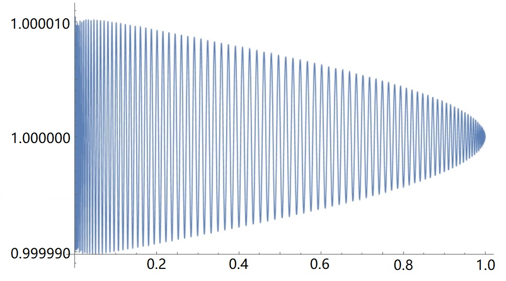
Figure 2: The sign function approximated by a Chebyshev polynomial with no more than $10^{-5}$ deviation.

For the Chebyshev polynomial, we estimate the ranks with an empirical formula, set several initial $x$ values and solve the equations of the coefficients to make the sign function at those values to be exact. Of course the residual will not vanish at the other points, and we need to repeat the procedure at the extreme points of the new polynomials until the precision goal is reached at the new extreme points. Note that one should use use the Clenshaw recursion to define the Chebyshev polynomial to suppress the round-off error.

In order to enhance the contribution from the low mode, the Chebyshev acceleration is also used in the eigenvector solver. Note that the polynomial will change the eigenvalues of a matrix, but its eigenvectors are kept unchanged.

One can apply the polynomial of a dslash several times on a random vector $b$ and obtain its Krylov array.

$${b,Ab,...,A^{k-1}b},$$ (6)

For Arnoldi algorithm, we can get a Heisenberg matrix after the Schmidt orthogonalization

$$AQ=\begin{pmatrix}Aq_{1}&Aq_{2}&\cdots&Aq_{k}\end{pmatrix}=\begin{pmatrix}q_{1}&q_{2}&\cdots&q_{k}\end{pmatrix}\begin{pmatrix}h_{1,1}&h_{1,2}&h_{1,3}&\cdots&h_{1,k}\\ h_{2,1}&h_{2,2}&h_{2,3}&\cdots&h_{2,k}\\ 0&h_{3,2}&h_{3,3}&\cdots&h_{3,k}\\ \vdots&\ddots&\ddots&\ddots&\vdots\\ 0&\cdots&0&h_{k,k-1}&h_{k,k}\end{pmatrix}.$$ (7)

Eventually the eigenvectors can be obtained by diagonalizing the Heisenberg matrix. Note that we can use the special QR factorization for Heisenberg matrix to suppress the round-off error. When the amount of the eigenvector is large, the restart algorithm is essential to save the GPU memory by the decrease of extra space.

As shown in Table 4, the GPU eigensolver can be much faster than the CPU one, on both the ensembles. Our codes use the restarted Arnoldi algorithm which is similar to the algorithm in the GWU-code.

tag	Ensembles	Number of eigenvectors	Nodes	time(Chroma)	time(GWU-code)
CPU	RBC11	200	1	8070s	-
GPU	RBC11	200	1	180s	225s
CPU	RBC08	200	4	4704s	-
GPU	RBC08	200	4	281s	317s

Table 4: The time needed to generate the 200 eigenvalues of $\gamma_{5}D_{w}$ with residual $10^{-15}$.

tag	Ensembles	Number of eigenvectors	Nodes	time(Chroma)	time(GWU-code)
CPU	RBC11	200	1	>12h	-
GPU	RBC11	200	1	7384s	16110s
CPU	RBC08	200	4	>12h	-
GPU	RBC08	200	4	8893s	14370s

Table 5: The time needed to generate the 200 eigenvalues of $D^{L/R}_{ov}$ with residual $10^{-12}$.

Similarly we can solve the low lying eigenvectors of the $D_{ov}$ to accelerate the inversion of the overlap propagator. Since the $D_{ov}$ is so-called gamma5 Hermite, we considered the projected $D^{L/R}_{ov}=(1\pm\gamma_{5})D_{ov}(1\pm\gamma_{5})$ to make sure that the eigenvalues are real for the convergence of the Arnoldi eigenslover and just solve the eigenvectors in the chiral sector with zero modes. In the end, we reconstruct the full spinor.

As in Table 5, the overlap eigensolver based on QUDA can be faster than our previous one using the GWU-code [9, 10]. On the RBC11 ensemble, 50 $D_{w}$ operations take 0.088s in GWU-code while just 0.025s in QUDA with 1 node, as we combine the $\gamma_{5}$ and $D_{w}$ operations into one kernel to save the bandwidth in the QUDA code, and QUDA can take advantage from its auto-tuning. But the cost of the vector operations are similar in both QUDA and GWU-code, thus the difference in the eigensolver performance is smaller, especially in the $H_{w}$ one which spends fewer time in the matrix operations. As a larger scale, the RBC08 ensemble uses 4 nodes and then the network has much stronger impact on the performance, so the $D_{w}$ performance in two cases are relatively closer, as 50 $D_{w}$ take 0.148s in GWU-code and 0.087s in QUDA.

We also implemented the deflation [1] and multi-mass [2] algorithm for the overlap propagator in Chroma to take the advantage of the overlap fermion definition. On the RBC11 ensembles, we generate overlap propagators with the mass of 0.03, 0.05 and 0.10 within the residual 1e-8. It takes 1150s in GWU-code while just 698s in QUDA with 1 node for the calculations. The RBC08 ensembles use 4 nodes and the speed up of the propagator solver is similar to that of $D_{ov}$ eigensolver. We choose the mass of the propagators as 0.03, 0.05 and 0.10 and the tolerance is set to be 1e-8. The inversion takes 1133s in GWU-code and 903s in QUDA. The performance in two cases are also closer.

3 Summary

In summary, we write the Chroma interfaces of the QUDA twist-mass and HISQ inverters, and implemented the overlap fermion eigensolver and inverter based on the QUDA dslash kernel and linear algebra operations. It turns out that the QUDA can provide significant speed up on the above three actions with the uniform Chroma interface, while that the HISQ multigrid solver would not be properly tuned and then require further efforts. It paves the way to compare the statistical and systematic uncertainties of the same physical observable with different actions, with an uniform environment.

References

- [1] A. Li et al. Overlap Valence on 2+1 Flavor Domain Wall Fermion Configurations with Deflation and Low-mode Substitution. Phys. Rev. D, 82:114501, 2010.
- [2] Beat Jegerlehner. Krylov space solvers for shifted linear systems. 12 1996.
- [3] E. Follana, Q. Mason, C. Davies, K. Hornbostel, G. P. Lepage, J. Shigemitsu, H. Trottier, and K. Wong. Highly improved staggered quarks on the lattice, with applications to charm physics. Phys. Rev. D, 75:054502, 2007.
- [4] Robert G. Edwards and Balint Joo. The Chroma software system for lattice QCD. Nucl. Phys. Proc. Suppl., 140:832, 2005. [,832(2004)].
- [5] M. A. Clark, Blint Jo, Alexei Strelchenko, Michael Cheng, Arjun Gambhir, and Richard Brower. Accelerating Lattice QCD Multigrid on GPUs Using Fine-Grained Parallelization. 2016.
- [6] Yu-Jiang Bi, Yi Xiao, Ming Gong, Wei-Yi Guo, Peng Sun, Shun Xu, and Yi-Bo Yang. Lattice QCD package GWU-code and QUDA with HIP. PoS, LATTICE2019:286, 2020.
- [7] M. A. Clark, R. Babich, K. Barros, R. C. Brower, and C. Rebbi. Solving Lattice QCD systems of equations using mixed precision solvers on GPUs. Comput. Phys. Commun., 181:1517–1528, 2010.
- [8] R. Babich, M. A. Clark, B. Joo, G. Shi, R. C. Brower, and S. Gottlieb. Scaling Lattice QCD beyond 100 GPUs. In SC11 International Conference for High Performance Computing, Networking, Storage and Analysis Seattle, Washington, November 12-18, 2011, 2011.
- [9] A. Alexandru, C. Pelissier, B. Gamari, and F. Lee. Multi-mass solvers for lattice QCD on GPUs. J. Comput. Phys., 231:1866–1878, 2012.
- [10] Andrei Alexandru, Michael Lujan, Craig Pelissier, Ben Gamari, and Frank X. Lee. Efficient implementation of the overlap operator on multi-GPUs. In Proceedings, 2011 Symposium on Application Accelerators in High-Performance Computing (SAAHPC’11): Knoxville, Tennessee, July 19-20, 2011, pages 123–130, 2011.
- [11] Richard C. Brower, M. A. Clark, Alexei Strelchenko, and Evan Weinberg. Multigrid algorithm for staggered lattice fermions. Phys. Rev. D, 97(11):114513, 2018.