Nonlinear $H_{\infty}$ Filtering on the Special Orthogonal Group $SO(3)$ using Vector Directions

Abstract

The problem of $H_{\infty}$ filtering for attitude estimation using rotation matrices and vector measurements is studied. Starting from a storage function on the Special Orthogonal Group $SO(3)$, a dissipation inequality is considered, and a deterministic nonlinear $H_{\infty}$ filter is derived which respects a given upper bound $\gamma$ on the energy gain from exogenous disturbances and initial estimation errors to a generalized estimation error. The results are valid for all estimation errors which correspond to an angular error of less than $\pi/2$ radians in terms of the axis-angle representation. The approach builds on earlier results on attitude estimation, in particular nonlinear $H_{\infty}$ filtering using quaternions, and proposes a novel filter developed directly on $SO(3)$. The proposed filter employs the same innovation term as the Multiplicative Extended Kalman Filter (MEKF), as well as a matrix gain updated in accordance with a Riccati-type gain update equation. However, in contrast to the MEKF, the proposed filter has an additional tuning gain, $\gamma$, which enables it to be more aggressive during transients. The filter is simulated for different conditions, and the results are compared with those obtained using the continuous-time quaternion MEKF and the Geometric Approximate Minimum Energy (GAME) filter. Simulations indicate competitive performance. In particular, the GAME filter has the best transient performance, followed by the proposed $H_{\infty}$ filter and the quaternion MEKF. All three filters have similar steady-state performance. Therefore, the proposed filter can be seen as a MEKF variant which achieves better transient performance without significant degradation in steady-state noise rejection.

Keywords— Attitude estimation, Special Orthogonal Group $SO(3)$, nonlinear $H_{\infty}$ filtering

1 Introduction

Rigid-body attitude estimation is a well-studied problem, and numerous solutions have been proposed [1, 2]. In general, attitude filtering problems are posed as optimization problems which seek to minimize a suitably defined cost function indicative of the filter’s performance. The cost function usually comprises a weighted average or integration of the estimation error, possibly with a terminal cost. For linear systems, most optimal filtering solutions are equivalent to Kalman filtering.

An alternative (pessimistic, or perhaps realistic) approach to attitude filtering is given by worst-case or nonlinear $H_{\infty}$ estimation. In formulating the $H_{\infty}$ filtering problem, one optimizes not for the average estimation error, but for the worst-case errors imparted by the worst-case disturbances and large initial estimation errors. The resulting filter respects a given upper bound on the energy gain from the disturbances and initial estimation errors to a chosen performance measure, also a function of the estimation error [3, 4, 5, 6, 7, 8].

Nonlinear $H_{\infty}$ filters have been applied successfully for spacecraft attitude determination using quaternions [2, 9, 10]. Since $H_{\infty}$ filters minimize only the worst-case error and not the mean square error (MSE), they are outperformed by the quaternion Multiplicative Extended Kalman Filter (MEKF), particularly in problem instances where the properties of the process and measurement noise/disturbance are perfectly known. However, for the more practical case of uncertain noise parameters leading to imperfect filter tuning, extensive Monte-Carlo simulations show that the MEKF gradually loses its edge, and that the $H_{\infty}$ filter performs better [11, 12]. Thus, nonlinear $H_{\infty}$ filtering offers a promising alternative to optimal estimation methods. Nevertheless, the quaternion MEKF remains the industry standard.

It is well-known that the attitude of a rigid body evolves on the set of rotation matrices, the Special Orthogonal Group $SO(3)$, and that all other attitude representations, including quaternions, suffer either from a singularity or a sign ambiguity [13]. Due to the globally defined and unique attitude representation provided by rotation matrices, the development of filtering solutions directly on the Lie group $SO(3)$ has received considerable attention in recent decades. The solutions proposed include nonlinear complementary filters [14, 15, 16, 17], symmetry-preserving observers [18, 19], the Invariant Extended Kalman Filter (IEKF) [20], and minimum energy filters [21, 22, 23, 24, 25]. Of these, the Geometric Approximate Minimum Energy (GAME) filter [24, 23], is especially relevant since it is an optimal estimation method that has been shown to significantly outperform the quaternion MEKF [26].

Given the potential benefits of worst-case filtering and the increasing interest in filtering algorithms on $SO(3)$, a promising solution might be to combine nonlinear $H_{\infty}$ filtering with attitude estimation using rotation matrices. This combination is the subject of the present work. We note that there has been some preliminary work in this direction. In particular, Lavoie et al. have proposed an invariant extended $H_{\infty}$ filter for Lie groups [27]. Noting the similarities and crucial differences between the Extended Kalman Filter (EKF) and its invariant counterpart, the IEKF, the authors consider an analogous relationship between the Extended $H_{\infty}$ Filter and its potential invariant counterpart. This simple and insightful observation leads them directly to an invariant extended $H_{\infty}$ filter for Lie groups. In contrast, we build on earlier results on nonlinear worst-case filtering using quaternions [9, 10], and extend them to the case of attitude estimation using rotation matrices. The main contribution of the paper is the development of a novel nonlinear $H_{\infty}$ filter on the Lie group $SO(3)$. It is envisaged that this exposition, which extends the preliminary results of [28], will pave the way for future developments, especially towards mixed $H_{2}/H_{\infty}$ filtering and possibly even the generalized $H_{\infty}$ regulator problem on $SO(3)$ yielding an estimator/controller pair which minimizes the impact of the worst-case disturbances on the controlled variables.

The rest of the discussion is organized as follows. After Section 1.1 introduces the notation used in the paper, Section 2 poses the $H_{\infty}$ filtering problem directly on $SO(3)$. Thereafter, the $H_{\infty}$ filter is derived in Section 3, and its structure is compared with that of the quaternion MEKF and the GAME filter. In Section 4, the proposed filter, the MEKF, and the GAME filter are simulated for different test conditions. Results indicate competitive performance. In particular, it is seen that the GAME filter has the best transient performance, whereas the $H_{\infty}$ filter demonstrates better convergence than the MEKF. At steady-state, the three filters have similar performance. Finally, in Section 5, the main conclusions of the study are reviewed.

1.1 Notation

The Special Orthogonal group $SO(3)$ is the set of $3\times 3$ orthogonal matrices with determinant $1$, i.e.,

$$SO(3) =\left\{R\in\mathbb{R}^{3\times 3}:R^{\top}R=I,\det\left(R\right)=1\right\}.$$

The cross operator $\times:\mathbb{R}^{3}\rightarrow\mathfrak{so}(3)$ transforms a vector in $\mathbb{R}^{3}$ to a $3$-by-$3$ skew-symmetric matrix such that $x^{\times}y$ equals the cross product $x\times y$ for any $x,y\in\mathbb{R}^{3}$. In particular,

$$x^{\times}=\begin{bmatrix}0&-x_{3}&x_{2}\\ x_{3}&0&-x_{1}\\ -x_{2}&x_{1}&0\end{bmatrix}.$$ (1)

The inverse of the cross operator is denoted by the vee operator $\vee:\mathfrak{so}(3)\rightarrow\mathbb{R}^{3}$. Lastly, we recall the symmetric projection operator $\mathbb{P}_{s}:\mathbb{R}^{n\times n}\rightarrow\mathbb{R}^{n\times n}$ given by

$$\mathbb{P}_{s}(M)=\frac{M+M^{\top}}{2}.$$ (2)

2 Problem Formulation

This section formulates the attitude estimation problem using rotation matrices. In particular, we assume the following kinematic model:

$$\begin{split}\dot{R}&=R(\omega+g\delta)^{\times}\\ y_{i}&=R^{\top}r_{i}+k_{i}\varepsilon_{i},\quad i=1,\ldots,p,\end{split}$$ (3)

where the state $R(t)$ evolves on $SO(3)$, and represents the orientation of a body-fixed frame with respect to an inertial reference frame. In the kinematics equation, the vectors $\omega,\delta\in\mathbb{R}^{3}$ are body-frame vectors denoting the measured angular velocity and the process disturbance, respectively. In the output equation, the vectors $\left\{r_{i}\right\}$ specify known vector directions in the reference frame, and the vectors $\left\{y_{i}\right\}$ represent their measurements in the body-fixed frame with corresponding measurement errors $\left\{\varepsilon_{i}\right\}$. Lastly, the coefficients $g$ and $\left\{k_{i}\right\}$ scale the process disturbance and measurement errors, respectively, and represent tuning gains for the filter proposed in Section 3.

We consider the following estimator:

$$\dot{\hat{R}} =\hat{R}\left(\omega+G_{q}\tilde{y}\right)^{\times}, \tilde{y}=\begin{bmatrix}y_{1}-\hat{y}_{1}\\ \vdots\\ y_{p}-\hat{y}_{p}\end{bmatrix},$$ (4)

where the filter gain $G_{q}\left(\hat{R},t\right)$ is a $3$-by-$3p$ matrix which will be specified later, and

$$\hat{y}_{i}=\hat{R}^{\top}r_{i},$$ (5)

represents the estimate for the $i$-th reference direction $r_{i}$. We note that this estimator structure is similar to the one considered in [9] for deriving a quaternion-based $H_{\infty}$ filter.

For the augmented system (3)-(4), the estimation error is defined as

$$\tilde{R}:=\hat{R}^{\top}R.$$ (6)

Using the axis-angle representation, the estimation error can be expressed as

$$\tilde{R} =I+\left(\sin\tilde{\theta}\right)e^{\times}+\left(1-\cos\tilde{\theta}\right)e^{\times}e^{\times},$$ (7)

where $e\in\mathbb{S}^{2}$ denotes the axis of rotation between the body-fixed and estimate frames, and $\tilde{\theta}$ denotes the angle of rotation. We consider the following configuration error vector as a penalty variable or generalized estimation error:

$$z :=\frac{1}{2}\left(\tilde{R}-\tilde{R}^{\top}\right)^{\vee}.$$ (8)

Using the axis-angle representation, the penalty variable can be expressed as

$$z=e\sin\tilde{\theta}.$$ (9)

We recall that the optimal $H_{\infty}$ filtering problem, for the augmented system (3)-(4), seeks a filter gain which minimizes the $\mathcal{L}_{2}$ gain from the process disturbance $\delta$, the measurement errors $\left\{\varepsilon_{i}\right\}$, and the initial conditions $R_{0}=R\left(0\right)$, $\hat{R}_{0}=\hat{R}\left(0\right)$ to the penalty variable $z\left(t\right)$. Since this is, in general, a difficult problem to solve, we resort to the sub-optimal $H_{\infty}$ filtering problem which ensures that the $\mathcal{L}_{2}$ gain respects a given upper bound $\gamma$, see e.g., [4, 5, 6, 9]. More precisely, we seek a filter gain such that for all $t\geq 0$, $\delta$, $\left\{\varepsilon_{i}\right\}$ , $R_{0}$, and $\hat{R}_{0}$, the following dissipation inequality is satisfied:

$$\int_{0}^{t}\left\|z\left(\tau\right)\right\|^{2}d\tau \leq\gamma^{2}\left\|z_{0}\right\|^{2}+\gamma^{2}\int_{0}^{t}\Bigl{[}\left\|\delta\left(\tau\right)\right\|^{2}$$ (10)

$$+\sum_{i}\left\|\varepsilon_{i}\right\|^{2}\Bigr{]}d\tau.$$

As has been well established in the literature on nonlinear $H_{\infty}$ control, see e.g., [3, 5, 6, 9, 10], the requirement (10) on the $\mathcal{L}_{2}$ gain is closely related to the notion of dissipativity. In particular, we seek a filter gain $G_{q}(\hat{R},t)$ and a smooth positive semidefinite storage function $V(R,\hat{R},t)$ such that the following dissipation inequality is satisfied:

$$\dot{V}\leq\gamma^{2}\left\|\delta\right\|^{2}+\gamma^{2}\sum_{i}\left\|\varepsilon_{i}\right\|^{2}-\left\|z\right\|^{2}.$$ (11)

Next, we obtain an expression for the time derivative of the penalty variable $z\left(t\right)$. In particular, from (8), we have that

$$z^{\times}=\frac{1}{2}\left(\tilde{R}-\tilde{R}^{\top}\right).$$ (12)

Conseqently, we can express the time derivative of the penalty variable as

$$\left(\dot{z}\right)^{\times}=\frac{1}{2}\left(\dot{\tilde{R}}-\dot{\tilde{R}}^{\top}\right).$$ (13)

Substituting the dynamics from (3) and (4), we can express the time derivative of $\tilde{R}$ as follows:

$$\dot{\tilde{R}} =\hat{R}^{\top}\dot{R}+\dot{\hat{R}}^{\top}R,$$

$$=\hat{R}^{\top}R\left(\omega+g\delta\right)^{\times}-\left(\omega+G_{q}\tilde{y}\right)^{\times}\hat{R}^{\top}R,$$

$$\implies\dot{\tilde{R}} =\tilde{R}\omega^{\times}-\omega^{\times}\tilde{R}+g\tilde{R}\delta^{\times}-\left(G_{q}\tilde{y}\right)^{\times}\tilde{R}.$$

Consequently, we have that:

$$\dot{\tilde{R}}-\dot{\tilde{R}}^{\top} =\left(\tilde{R}\omega^{\times}+\omega^{\times}\tilde{R}^{\top}\right)-\left(\omega^{\times}\tilde{R}+\tilde{R}^{\top}\omega^{\times}\right)$$

$$\quad+g\left(\tilde{R}\delta^{\times}+\delta^{\times}\tilde{R}^{\top}\right)-\left(\left(G_{q}\tilde{y}\right)^{\times}\tilde{R}+\tilde{R}^{\top}\left(G_{q}\tilde{y}\right)^{\times}\right).$$

We apply the following identity to each term on the right-hand side of the above expression:

$$x^{\times}A+A^{\top}x^{\times}=\left(\left\{\text{tr}[A]I-A\right\}x\right)^{\times},\quad x\in\mathbb{R}^{3},A\in\mathbb{R}^{3\times 3}.$$

For the first two terms, we observe that:

$$\left(\tilde{R}\omega^{\times}+\omega^{\times}\tilde{R}^{\top}\right)-\left(\omega^{\times}\tilde{R}+\tilde{R}^{\top}\omega^{\times}\right)$$

$$= \left(\left(\text{tr}\left[\tilde{R}^{\top}\right]I-\tilde{R}^{\top}-\text{tr}\left[\tilde{R}\right]I+\tilde{R}\right)\omega\right)^{\times},$$

$$= \left(\left(\tilde{R}-\tilde{R}^{\top}\right)\omega\right)^{\times},$$

$$= 2\left(z^{\times}\omega\right)^{\times},$$

In the above simplification, the last equality follows from the relation (12). Next, we introduce the following mapping:

$$\textbf{E}\left(M\right):=\text{tr}\left[M\right]I-M^{\top}.$$ (14)

Consequently, we can express (13) as:

$$\left(\dot{z}\right)^{\times}=\left(z^{\times}\omega\right)^{\times}+\frac{g}{2}\left(\textbf{E}\left(\tilde{R}\right)\delta\right)^{\times}-\frac{1}{2}\left(\textbf{E}^{\top}\left(\tilde{R}\right)G_{q}\tilde{y}\right)^{\times}.$$

Removing the $\times$ operator, and substituting for $\tilde{y}$ and $\hat{y}_{i}$ from (4)-(5), we obtain:

$$\dot{z} =z^{\times}\omega+\frac{g}{2}\textbf{E}\left(\tilde{R}\right)\delta-\frac{1}{2}\textbf{E}^{\top}\left(\tilde{R}\right)G_{q}\begin{bmatrix}R^{\top}r_{1}-\hat{R}^{\top}r_{1}\\ \vdots\\ R^{\top}r_{p}-\hat{R}^{\top}r_{p}\end{bmatrix}$$

$$\quad-\frac{1}{2}\textbf{E}^{\top}\left(\tilde{R}\right)G_{q}\begin{bmatrix}k_{1}\varepsilon_{1}\\ \vdots\\ k_{p}\varepsilon_{p}\end{bmatrix}.$$ (15)

3 Filter Derivation

This section presents a novel $H_{\infty}$ filter for attitude estimation using rotation matrices. The filter derivation follows the same procedure as is used in [9, 10] for deriving a quaternion-based $H_{\infty}$ filter. In particular, starting from a storage function on $SO\left(3\right)$, a dissipation inequality of the form (11) is considered. The worst-case process disturbance and measurement errors are obtained, as well as the gain which optimizes for the worst-case disturbances. These values are used to simplify the dissipation inequality. Thereafter, for sufficiently small estimation errors, a deterministic nonlinear $H_{\infty}$ filter is derived, the filter gain $G_{q}$ is specified, and a Riccati-type gain update equation is obtained.

We consider the following storage function:

$$V(R,\hat{R},t)=\gamma^{2}z^{\top}P^{-1}(t)z,$$ (16)

where the penalty variable $z(t)$ is defined as in (8), and $P(t)$ is a symmetric, positive definite, $3$-by-$3$ matrix. The time derivative of the storage function is given by

$$\dot{V}=-\gamma^{2}z^{\top}P^{-1}\dot{P}P^{-1}z+2\gamma^{2}z^{\top}P^{-1}\dot{z}.$$ (17)

Substituting (15) in (17), the dissipation inequality (11) can be expressed as:

$$-\gamma^{2}z^{\top}P^{-1}\dot{P}P^{-1}z-2\gamma^{2}z^{\top}P^{-1}\omega^{\times}z$$

$$+g\gamma^{2}z^{\top}P^{-1}\textbf{E}\left(\tilde{R}\right)\delta$$

$$-\gamma^{2}z^{\top}P^{-1}\textbf{E}^{\top}\left(\tilde{R}\right)G_{q}\begin{bmatrix}R^{\top}r_{1}-\hat{R}^{\top}r_{1}\\ \vdots\\ R^{\top}r_{p}-\hat{R}^{\top}r_{p}\end{bmatrix}$$

$$-\gamma^{2}z^{\top}P^{-1}\textbf{E}^{\top}\left(\tilde{R}\right)G_{q}\begin{bmatrix}k_{1}\varepsilon_{1}\\ \vdots\\ k_{p}\varepsilon_{p}\end{bmatrix}$$

$$-\gamma^{2}\left\|\delta\right\|^{2}-\gamma^{2}\sum_{i}\left\|\varepsilon_{i}\right\|^{2}+z^{\top}z\leq 0.$$ (18)

Remark 1.

Using the axis-angle representation (9) of the penalty variable, the storage function (16) can be expressed as

$$V=\gamma^{2}\left(\sin^{2}\tilde{\theta}\right)e^{\top}P^{-1}e.$$ (19)

Thus, we have that the angular term increases only in the interval $|\tilde{\theta}|\in\left(0,\frac{\pi}{2}\right)$ and decreases to $0$ thereafter. This means that although the storage function is nonnegative, it can be used to obtain stability and performance guarantees only for angular errors up to $\pi/2$ radians. Having noted this limitation, we now proceed to the main steps in the filter derivation.

3.1 Worst-case Disturbances

The dissipation inequality (18) is quadratic in the process disturbance $\delta$ and the measurement errors $\left\{\varepsilon_{i}\right\}$. In particular, the worst-case process disturbance can be obtained as follows:

$$g\gamma^{2}\textbf{E}^{\top}\left(\tilde{R}\right)P^{-1}z-2\gamma^{2}\delta^{*}=0,$$

$$\implies\delta^{*}=\frac{g}{2}\textbf{E}^{\top}\left(\tilde{R}\right)P^{-1}z.$$ (20)

Its contribution to the dissipation inequality (18) is given by the term

$$\frac{\gamma^{2}g^{2}}{4}z^{\top}P^{-1}\textbf{E}\left(\tilde{R}\right)\textbf{E}^{\top}\left(\tilde{R}\right)P^{-1}z.$$

Next, we partition the filter gain $G_{q}$ as

$$G_{q}=\begin{bmatrix}G_{q,1}&\cdots&G_{q,p}\end{bmatrix},$$

where $G_{q,i}\in\mathbb{R}^{3\times 3}$. Then, the $i$-th worst-case measurement error can be obtained as:

$$-k_{i}\gamma^{2}G_{q,i}^{\top}\textbf{E}\left(\tilde{R}\right)P^{-1}z-2\gamma^{2}\varepsilon_{i}^{*}=0,$$

$$\implies\varepsilon_{i}^{*}=-\frac{k_{i}}{2}G_{q,i}^{\top}\textbf{E}\left(\tilde{R}\right)P^{-1}z.$$ (21)

Its contribution to (18) is given by

$$\frac{\gamma^{2}k_{i}^{2}}{4}z^{\top}P^{-1}\textbf{E}^{\top}\left(\tilde{R}\right)G_{q,i}G_{q,i}^{\top}\textbf{E}\left(\tilde{R}\right)P^{-1}z,$$

and the total contribution of the worst-case measurement errors $\left\{\varepsilon_{i}^{*}\right\}$ is given by

$$\frac{\gamma^{2}}{4}z^{\top}P^{-1}\textbf{E}^{\top}\left(\tilde{R}\right)G_{q}KG_{q}^{\top}\textbf{E}\left(\tilde{R}\right)P^{-1}z,$$

where

$$K:=\text{diag}\left[k_{1}^{2}I,\ldots,k_{p}^{2}I\right]\in\mathbb{R}^{3p\times 3p}.$$ (22)

Consequently, after substituting the worst-case process disturbance $\delta^{*}$ and the worst-case measurement errors $\left\{\varepsilon_{i}^{*}\right\}$, we arrive at the following dissipation inequality:

$$-\gamma^{2}z^{\top}P^{-1}\dot{P}P^{-1}z-2\gamma^{2}z^{\top}P^{-1}\omega^{\times}z$$

$$+\frac{\gamma^{2}g^{2}}{4}z^{\top}P^{-1}\textbf{E}\left(\tilde{R}\right)\textbf{E}^{\top}\left(\tilde{R}\right)P^{-1}z$$

$$-\gamma^{2}z^{\top}P^{-1}\textbf{E}^{\top}\left(\tilde{R}\right)G_{q}\begin{bmatrix}R^{\top}r_{1}-\hat{R}^{\top}r_{1}\\ \vdots\\ R^{\top}r_{p}-\hat{R}^{\top}r_{p}\end{bmatrix}$$

$$+\frac{\gamma^{2}}{4}z^{\top}P^{-1}\textbf{E}^{\top}\left(\tilde{R}\right)G_{q}KG_{q}^{\top}\textbf{E}\left(\tilde{R}\right)P^{-1}z$$

$$+z^{\top}z\leq 0.$$ (23)

3.2 Filter Gain

In order to find the optimal filter gain for the worst-case disturbances, we perform completion of squares for the terms in the dissipation inequality (23) that contain the gain $G_{q}$. In particular, these terms can be re-stated as:

$$\frac{\gamma^{2}}{4}\left\|K^{1/2}G_{q}^{\top}\textbf{E}\left(\tilde{R}\right)P^{-1}z-2K^{-1/2}\begin{bmatrix}R^{\top}r_{1}-\hat{R}^{\top}r_{1}\\ \vdots\\ R^{\top}r_{p}-\hat{R}^{\top}r_{p}\end{bmatrix}\right\|^{2}$$

$$-\gamma^{2}\begin{bmatrix}R^{\top}r_{1}-\hat{R}^{\top}r_{1}\\ \vdots\\ R^{\top}r_{p}-\hat{R}^{\top}r_{p}\end{bmatrix}^{\top}K^{-1}\begin{bmatrix}R^{\top}r_{1}-\hat{R}^{\top}r_{1}\\ \vdots\\ R^{\top}r_{p}-\hat{R}^{\top}r_{p}\end{bmatrix}.$$

Therefore, the gain $G_{q}$ which minimizes the left-hand side of (23) satisfies the following condition:

$$z^{\top}P^{-1}\textbf{E}^{\top}\left(\tilde{R}\right)G_{q}=2\begin{bmatrix}R^{\top}r_{1}-\hat{R}^{\top}r_{1}\\ \vdots\\ R^{\top}r_{p}-\hat{R}^{\top}r_{p}\end{bmatrix}^{\top}K^{-1}.$$ (24)

Substituting $\hat{y}_{i}$ and $\tilde{R}$ from (5)-(6), we observe that:

$$R^{\top}r_{i}-\hat{R}^{\top}r_{i}=\left(R^{\top}\hat{R}-I\right)\hat{R}^{\top}r_{i}=\left(\tilde{R}^{\top}-I\right)\hat{y}_{i}.$$

Furthermore, using the axis-angle representations (7) and (9), and assuming that $\cos\tilde{\theta}\neq-1$, we proceed as follows:

$$\left(\tilde{R}^{\top}-I\right)\hat{y}_{i} =\left[\left(1-\cos\tilde{\theta}\right)e^{\times}e^{\times}-\left(\sin\tilde{\theta}\right)e^{\times}\right]\hat{y}_{i},$$

$$=\left[\left(\frac{\sin\tilde{\theta}}{1+\cos\tilde{\theta}}\right)e^{\times}-I\right]\left(\sin\tilde{\theta}\right)e^{\times}\hat{y}_{i},$$

$$=\left(\frac{1}{1+\cos\tilde{\theta}}z^{\times}-I\right)z^{\times}\hat{y}_{i},$$

$$=-\left(\frac{1}{1+\cos\tilde{\theta}}z^{\times}-I\right)\left(\hat{y}_{i}\right)^{\times}z.$$ (25)

Therefore, using the preceding relations, the minimizing gain condition can be expressed as follows:

$$z^{\top}P^{-1}\textbf{E}^{\top}\left(\tilde{R}\right)G_{q} =-2z^{\top}\left[\begin{array}[]{cc}\left(\hat{y}_{1}\right)^{\times}\left(\frac{1}{1+\cos\tilde{\theta}}z^{\times}+I\right)&\cdots\end{array}\right.$$

$$\left.\begin{array}[]{cc}\ldots&\left(\hat{y}_{p}\right)^{\times}\left(\frac{1}{1+\cos\tilde{\theta}}z^{\times}+I\right)\end{array}\right]K^{-1}.$$

This leads to the following sufficient condition for the minimizing gain:

$$\textbf{E}^{\top}\left(\tilde{R}\right)G_{q} =-2P\left(t\right)\left[\begin{array}[]{cc}\left(\hat{y}_{1}\right)^{\times}\left(\frac{1}{1+\cos\tilde{\theta}}z^{\times}+I\right)&\cdots\end{array}\right.$$

$$\left.\begin{array}[]{cc}\ldots&\left(\hat{y}_{p}\right)^{\times}\left(\frac{1}{1+\cos\tilde{\theta}}z^{\times}+I\right)\end{array}\right]K^{-1}.$$

We note that this condition couples the gain matrix $G_{q}$ to the true estimation error $\tilde{R}=\hat{R}^{\top}R$, and that the latter cannot be computed since the true trajectory $R(t)$ is not available. However, an approximate solution may be obtained for small estimation errors, i.e., for $\hat{R}(t)\approx R(t)$. In particular, as $\tilde{R}(t)\rightarrow I$, we have that the penalty variable $z\rightarrow 0$, the mapping $\textbf{E}\left(\tilde{R}\right)\rightarrow 2I$, and the sufficient condition for the minimizing gain simplifies thus:

$$G_{q}\left(\hat{R},t\right) =-P\left(t\right)\begin{bmatrix}\left(\hat{R}^{\top}r_{1}\right)^{\times}&\ldots&\left(\hat{R}^{\top}r_{p}\right)^{\times}\end{bmatrix}K^{-1}$$

$$=P\left(t\right)H^{\top}\left(\hat{R},r\right)K^{-1},$$ (26)

where

$$H\left(\hat{R},r\right):=\begin{bmatrix}\left(\hat{R}^{\top}r_{1}\right)^{\times}\\ \vdots\\ \left(\hat{R}^{\top}r_{p}\right)^{\times}\end{bmatrix}.$$ (27)

Consequently, substituting $K$ and $G_{q}$ from (22) and (26), we obtain the following expression for the estimator (4):

$$\dot{\hat{R}}=\hat{R}\left(\omega-P\left(t\right)\sum_{i}k_{i}^{-2}\left(\hat{R}^{\top}r_{i}\right)\times y_{i}\right)^{\times}.$$ (28)

We note that the same estimator structure is used in [22], and admits, as special cases, the structures employed in [15, 17] for attitude estimation using vector measurements.

3.3 Gain Update Equation

This section derives a Riccati-type gain update equation for the time-varying filter gain $P\left(t\right)$ in the estimator (28). Substituting the minimizing gain condition (24) in the dissipation inequality (23) leads to the following expression:

$$-\gamma^{2}z^{\top}P^{-1}\dot{P}P^{-1}z-2\gamma^{2}z^{\top}P^{-1}\omega^{\times}z$$

$$-\gamma^{2}\begin{bmatrix}R^{\top}r_{1}-\hat{R}^{\top}r_{1}\\ \vdots\\ R^{\top}r_{p}-\hat{R}^{\top}r_{p}\end{bmatrix}^{\top}K^{-1}\begin{bmatrix}R^{\top}r_{1}-\hat{R}^{\top}r_{1}\\ \vdots\\ R^{\top}r_{p}-\hat{R}^{\top}r_{p}\end{bmatrix}$$

$$+\frac{\gamma^{2}g^{2}}{4}z^{\top}P^{-1}\textbf{E}\left(\tilde{R}\right)\textbf{E}^{\top}\left(\tilde{R}\right)P^{-1}z$$

$$+z^{\top}z\leq 0$$ (29)

The next step is to re-state each term in the above dissipation inequality using the axis-angle representation $\left(e,\tilde{\theta}\right)$ for the estimation error $\tilde{R}$. For the second term , we observe that:

$$-2\gamma^{2}z^{\top}P^{-1}\omega^{\times}z =-\gamma^{2}z^{\top}P^{-1}\omega^{\times}z+\gamma^{2}z^{\top}\omega^{\times}P^{-1}z$$

$$=\gamma^{2}z^{\top}\left(\omega^{\times}P^{-1}-P^{-1}\omega^{\times}\right)z$$

$$=\gamma^{2}\left(\sin^{2}\tilde{\theta}\right)e^{\top}\left(\omega^{\times}P^{-1}-P^{-1}\omega^{\times}\right)e$$ (30)

In order to simplify the third term in (29), we recall the relation (25) and the following identities:

$$z^{\times}z^{\times} =zz^{\top}-\left(\sin^{2}\tilde{\theta}\right)I, z^{\top}z^{\times}=0.$$

Assuming that $\cos\tilde{\theta}\neq-1$, we proceed as follows:

$$\left(R^{\top}r_{i}-\hat{R}^{\top}r_{i}\right)^{\top}\left(R^{\top}r_{i}-\hat{R}^{\top}r_{i}\right)$$

$$=z^{\top}\left(\hat{R}^{\top}r_{i}\right)^{\times}\left(\frac{1}{\left(1+\cos\tilde{\theta}\right)^{2}}z^{\times}z^{\times}-I\right)\left(\hat{R}^{\top}r_{i}\right)^{\times}z$$

$$=\left(-\frac{\sin^{2}\tilde{\theta}}{\left(1+\cos\tilde{\theta}\right)^{2}}-1\right)z^{\top}\left(\hat{R}^{\top}r_{i}\right)^{\times}\left(\hat{R}^{\top}r_{i}\right)^{\times}z$$

$$=-\frac{2}{1+\cos\tilde{\theta}}z^{\top}\left(\hat{R}^{\top}r_{i}\right)^{\times}\left(\hat{R}^{\top}r_{i}\right)^{\times}z$$

$$=-2\left(1-\cos\tilde{\theta}\right)e^{\top}\left(\hat{R}^{\top}r_{i}\right)^{\times}\left(\hat{R}^{\top}r_{i}\right)^{\times}e$$

Consequently, using the axis-angle representation and the definition of $H$ in (27), the third term in (29) can be simplified as follows:

$$-\gamma^{2}\begin{bmatrix}R^{\top}r_{1}-\hat{R}^{\top}r_{1}\\ \vdots\\ R^{\top}r_{p}-\hat{R}^{\top}r_{p}\end{bmatrix}^{\top}K^{-1}\begin{bmatrix}R^{\top}r_{1}-\hat{R}^{\top}r_{1}\\ \vdots\\ R^{\top}r_{p}-\hat{R}^{\top}r_{p}\end{bmatrix}$$

$$=2\gamma^{2}\left(1-\cos\tilde{\theta}\right)e^{\top}\left(\sum_{i}k_{i}^{-2}\left(\hat{R}^{\top}r_{i}\right)^{\times}\left(\hat{R}^{\top}r_{i}\right)^{\times}\right)e$$

$$=-2\gamma^{2}\left(1-\cos\tilde{\theta}\right)e^{\top}H^{\top}K^{-1}He$$ (31)

For the fourth term in (29), we recall the map (14) and proceed as follows:

$$\textbf{E}\left(\tilde{R}\right)\textbf{E}^{\top}\left(\tilde{R}\right) =\text{tr}^{2}\left[\tilde{R}\right]I-\text{tr}\left[\tilde{R}\right]\left(\tilde{R}+\tilde{R}^{\top}\right)+I$$

$$=I+\text{tr}\left[\tilde{R}\right]\left[\text{tr}\left[\tilde{R}\right]I-\left(\tilde{R}+\tilde{R}^{\top}\right)\right]$$

Using the axis-angle representation (7), we observe that:

$$\text{tr}\left[\tilde{R}\right]I-\left(\tilde{R}+\tilde{R}^{\top}\right)$$

$$=\left(1+2\cos\tilde{\theta}\right)I-2\left[I+\left(1-\cos\tilde{\theta}\right)e^{\times}e^{\times}\right]$$

$$=\left(2\cos\tilde{\theta}-1\right)I-2\left(1-\cos\tilde{\theta}\right)e^{\times}e^{\times}$$

$$=\left(2\cos\tilde{\theta}-1\right)I-2\left(1-\cos\tilde{\theta}\right)\left(ee^{\top}-I\right)$$

$$=I-2\left(1-\cos\tilde{\theta}\right)ee^{\top}$$

Therefore:

$$\textbf{E}\left(\tilde{R}\right)\textbf{E}^{\top}\left(\tilde{R}\right) =2\left(1+\cos\tilde{\theta}\right)I$$

$$\quad-2\left(1+2\cos\tilde{\theta}\right)\left(1-\cos\tilde{\theta}\right)ee^{\top}$$

Consequently, the fourth term in (29) can be expressed as follows:

$$\frac{\gamma^{2}g^{2}}{2}\left[\left(1+\cos\tilde{\theta}\right)\left(\sin^{2}\tilde{\theta}\right)e^{\top}P^{-2}e\right.$$

$$\left.-\left(1+2\cos\tilde{\theta}\right)\left(1-\cos\tilde{\theta}\right)\left(\sin^{2}\tilde{\theta}\right)\left(e^{\top}P^{-1}e\right)^{2}\right]$$ (32)

Finally, using (30)-(32), we re-state the dissipation inequality (29) in terms of the axis-angle representation as follows:

$$-\gamma^{2}\left(\sin^{2}\tilde{\theta}\right)e^{\top}P^{-1}\dot{P}P^{-1}e$$

$$+\gamma^{2}\left(\sin^{2}\tilde{\theta}\right)e^{\top}\left(\omega^{\times}P^{-1}-P^{-1}\omega^{\times}\right)e$$

$$-2\gamma^{2}\left(1-\cos\tilde{\theta}\right)e^{\top}H^{\top}K^{-1}He$$

$$+\frac{\gamma^{2}g^{2}}{2}\left(1+\cos\tilde{\theta}\right)\left(\sin^{2}\tilde{\theta}\right)e^{\top}P^{-2}e+\left(\sin^{2}\tilde{\theta}\right)e^{\top}e$$

$$-\frac{\gamma^{2}g^{2}}{2}\left(1+2\cos\tilde{\theta}\right)\left(1-\cos\tilde{\theta}\right)\left(\sin^{2}\tilde{\theta}\right)\left(e^{\top}P^{-1}e\right)^{2}\leq 0$$ (33)

In the above dissipation inequality, the first five terms are second-order in the Euler axis $e$, the last term is fourth-order, and the coefficient of the last term is positive for $|\tilde{\theta}|\leq 120^{\circ}$. Furthermore, we observe that:

$$\frac{1}{2}\sin^{2}\tilde{\theta}\leq 1-\cos\tilde{\theta}$$

Therefore, for $|\tilde{\theta}|\leq 90^{\circ}$, a sufficient condition for the dissipation inequality (33) to hold is given as follows:

$$-\gamma^{2}\left(\sin^{2}\tilde{\theta}\right)e^{\top}P^{-1}\dot{P}P^{-1}e$$

$$+\gamma^{2}\left(\sin^{2}\tilde{\theta}\right)e^{\top}\left(\omega^{\times}P^{-1}-P^{-1}\omega^{\times}\right)e$$

$$-\gamma^{2}\left(\sin^{2}\tilde{\theta}\right)e^{\top}H^{\top}K^{-1}He$$

$$+\gamma^{2}g^{2}\left(\sin^{2}\tilde{\theta}\right)e^{\top}P^{-2}e+\left(\sin^{2}\tilde{\theta}\right)e^{\top}e\leq 0$$

Dividing throughout by $\gamma^{2}\left(\sin^{2}\tilde{\theta}\right)$ and considering only the matrix-valued terms, we obtain the following Riccati-type update equation for the filter gain $P\left(t\right)$:

$$\dot{P} =P\omega^{\times}-\omega^{\times}P-PH^{\top}K^{-1}HP+g^{2}I+\frac{1}{\gamma^{2}}P^{2}$$

Substituting for $\hat{y}_{i}$ and $H$ from (5) and (27), respectively, we summarize the equations for the continuous-time $H_{\infty}$ filter on $SO\left(3\right)$ as follows:

$$\begin{split}\dot{\hat{R}}&=\hat{R}\left(\omega-Pl\right)^{\times},\quad l=\sum_{i}k_{i}^{-2}\left(\hat{y}_{i}\times y_{i}\right)\\ \dot{P}&=\mathbb{P}_{s}\left(2P\omega^{\times}\right)+P\left(\sum_{i}k_{i}^{-2}\hat{y}_{i}^{\times}\hat{y}_{i}^{\times}\right)P+g^{2}I+\frac{1}{\gamma^{2}}P^{2},\end{split}$$ (34)

where $\mathbb{P}_{s}$ denotes the symmetric projection operator (2). We note that the gain update equation is similar to that proposed for the quaternion $H_{\infty}$ filter [9, 10].

Remark 2.

The proposed $H_{\infty}$ filter (34) is similar to the quaternion MEKF [29] and the quaternion left-invariant EKF (LIEKF) [30]. More precisely, suppose that in the kinematic system under consideration (3), the process disturbance $\delta$ and the measurement errors $\left\{\varepsilon_{i}\right\}$ are zero-mean Gaussian noises with standard deviations $\sigma_{\omega}$ and $\left\{\sigma_{i}\right\}$, respectively. Then, the continuous-time quaternion MEKF [29], which also coincides with the continuous-time quaternion LIEKF [30], can be expressed as:

$$\begin{split}\frac{d}{dt}\begin{bmatrix}\hat{q}_{v}\\ \hat{q}_{s}\end{bmatrix}&=\frac{1}{2}\begin{bmatrix}\hat{q}_{s}I+\hat{q}_{v}^{\times}\\ -\hat{q}_{v}^{\top}\end{bmatrix}\omega_{\text{ref}},\\ \omega_{\text{ref}}&=\omega-P\sum_{i}\sigma_{i}^{-2}\left(\hat{y}_{i}\times y_{i}\right),\end{split}$$ (35)

where

$$\hat{R}=\left(\hat{q}_{s}^{2}-\hat{q}_{v}^{\top}\hat{q}_{v}\right)I+2\hat{q}_{v}\hat{q}_{v}^{\top}+2\hat{q}_{s}\hat{q}_{v}^{\times},$$ (36)

and the filter gain is updated as follows:

$$\dot{P}=\mathbb{P}_{s}\left(2P\omega^{\times}\right)+P\left(\sum_{i}\sigma_{i}^{-2}\hat{y}_{i}^{\times}\hat{y}_{i}^{\times}\right)P+\sigma_{\omega}^{2}I.$$ (37)

Comparing (34) and (35)-(37), we note that the proposed $H_{\infty}$ filter and the continuous-time quaternion MEKF/LIEKF use identical innovation terms. Likewise, the gain update equations are similar except that the proposed $H_{\infty}$ filter has an additional second-order term containing $\gamma$. This term can be seen as an extra tuning gain which can be used to make the filter more aggressive during transients. Therefore, the proposed filter can be seen as a MEKF variant which achieves better transient performance without significant degradation in steady-state noise rejection. Moreover, this term vanishes in the limit $\gamma\rightarrow\infty$.

Remark 3.

The vector directions $H_{\infty}$ filter (34) can also be compared with the Geometric Approximate Minimum Energy (GAME) filter [22, 24]. The GAME filter is especially relevant since it is an optimal estimation method that has been shown to significantly outperform the quaternion MEKF [26]. For the kinematic system under consideration (3), the GAME filter [24, Section 4.3], [31] can be expressed as:

$$\begin{split}\dot{\hat{R}}&=\hat{R}\left(\omega-Pl\right)^{\times},\quad l=\sum_{i}k_{i}^{-2}\left(\hat{y}_{i}\times y_{i}\right),\\ \dot{P}&=\mathbb{P}_{s}\left(2P\omega^{\times}\right)+P\left(\sum_{i}k_{i}^{-2}\hat{y}_{i}^{\times}\hat{y}_{i}^{\times}\right)P+g^{2}I\\ &\quad-\mathbb{P}_{s}\left(P\left(Pl\right)^{\times}\right)+P\;\textbf{E}\left(\sum_{i}\mathbb{P}_{s}\left(k_{i}^{-2}\left(\hat{y}_{i}-y_{i}\right)y_{i}^{\top}\right)\right)P,\end{split}$$ (38)

where the map E is given in (14). We note that the $H_{\infty}$ and GAME filters use the same innovation terms, but differ significantly in their gain update equations. More precisely, the $H_{\infty}$ filter contains a $\gamma$-related term, whereas the GAME filter contains geometric curvature correction terms which enable it to have better transient performance than the MEKF.

Remark 4.

As mentioned earlier, the storage function (19) can be used to obtain stability and performance guarantees only for angular errors up to $\pi/2$ radians. A better starting point would be to assume a storage function which is strictly increasing in the angular error. More precisely, consider the following chordal metric-based storage function:

$$V_{\text{ch}}\left(R,\hat{R},t\right)=\frac{\gamma^{2}}{2}\text{tr}\left[P^{-1}\left(t\right)\left(I-\hat{R}^{\top}R\right)\right]$$ (39)

From [32, Lemma 2.2.5], we observe that

$$V_{\text{ch}}=\frac{1}{2}\gamma^{2}\left(1-\cos\tilde{\theta}\right)e^{\top}\textbf{E}\left(P^{-1}\right)e,$$ (40)

where the map E is given in (14). We note that a similar function is used in [21] for deriving a minimum energy filter on $SO(3)$. In future work, we hope to re-visit the problem of worst-case $H_{\infty}$ estimation using a chordal metric-based storage function.

4 Simulation Results

In this section we simulate the proposed filter (34), as well as the GAME filter and the MEKF, against different test cases and compare their performance. The proposed filter and the minimum energy filter are both implemented using a full rotation matrix representation for the state with vector measurements, while the MEKF is implemented in using the quaternion representation and vector measurements (35)-(37).

Two different test cases are considered. In Section 4.1 we consider a simulation case whose parameters are motivated by the characteristics of a typical inertial measurement unit (IMU) used in small quad-rotors. In Section 4.2, the test case is characterized by a relatively higher process (i.e., gyro) noise but lower measurement noise.

4.1 Case A

The true trajectory of the system is generated using

$$\dot{R} =R\omega_{\text{true}}^{\times}, R\left(0\right)=R_{0},$$

where $R_{0}$ is the rotation matrix corresponding to the Euler angles $\begin{bmatrix}\pi&-\frac{\pi}{2}&\frac{\pi}{2}\end{bmatrix}^{\top}$, and $\omega_{\text{true}}$ is the true angular velocity, given by

$$\omega_{\text{true}} =\begin{bmatrix}\cos 3t\\ 0.1\sin 2t\\ -\cos t\end{bmatrix}\text{rad/s}.$$

The angular velocity signal is then integrated to obtain the true trajectory of the state on $SO(3)$. This true trajectory, see Figure 1, is clearly simulating a large movement on $SO(3)$. The filter, however, only has been provided with the corrupted angular velocity signal, similar to the case of gyroscopic measurements of angular rate. The process disturbance corrupting the true angular velocity is generated by a vector of three independent sources of zero-mean white noises having standard deviations of $\sqrt{\pi/12}$ rad/s. The measurement disturbance vectors are obtained by generating two sets of the three independent realizations of zero-mean white noises having standard deviations of $\sqrt{\pi/12}$ rad. The system and the filters are both simulated with a time step of 0.01 seconds (i.e., at 100 Hz), and for a total simulation time of 30 seconds.

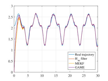
Figure 1: True and estimated trajectories (Case A)

To get a better insight into the convergence and tracking performance of the filters, the system model is initialized with a large initial attitude, equivalent to the Euler angles $\begin{bmatrix}\pi&-\frac{\pi}{2}&\frac{\pi}{2}\end{bmatrix}^{T}$. The filters are however assumed to have no prior knowledge of the initial attitude, and to cope with this uncertainty the initial gain is set to a large value, i.e., $P_{0}=\frac{1}{2}I$. The MEKF is tuned with the true parameters of process and measurement disturbance. Although the proposed $H_{\infty}$ filter and the GAME filter are deterministic filters, the knowledge of process and measurement noises can still be used to tune these filters. Hence, we choose $g=\sigma_{\delta}$ and $k_{i}=\sigma_{\epsilon}$ for both of these filters. Furthermore, for the $H_{\infty}$ filter, $\gamma=0.9$ is found to offer a good trade-off between stability and speed of convergence. While decreasing $\gamma$ further means a tighter bound on the $L_{2}$ error gain, it is to be reminded that a solution of the Riccati equation (34) may cease to exist for too small values of $\gamma$, see e.g., [33, 34].

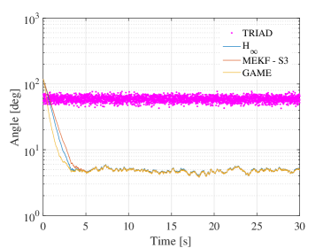
Figure 2: Measurement and estimation errors - RMS values (Case A)

Table 1: Estimation errors (deg) for Case A

	Transient	Steady state
	RMS error	RMS error
TRIAD	59.52	59.29
MEKF	27.79	4.74
$H_{\infty}$ Filter	26.24	4.79
GAME	21.68	4.73

The absolute values of the estimation errors are averaged over 50 runs to obtain the plots of estimation error, see Figure 2, and to compute the normalized RMS error in Table 1. The RMS error is split in two parts: the transient part during the first 10 seconds and the steady state part after the transient part. The results suggest that the GAME filter demonstrates the best performance during the transients while the proposed filter (34) performs slightly better than the MEKF. All the filters seem to exhibit similar performance at the steady-state. We conjecture that its the effect of geometric curvature terms in the Riccati equation (38), which makes the GAME filter more agile during the transients.

4.2 Case B

Now we consider another case which is characterized by a high process noise (which signifies a less accurate system model) but a low measurement noise. The same simulation setup is maintained as in Section 4.1, except that process and measurement disturbances are taken to be $2\cdot\sqrt{\pi/12}$ rad/s and $\frac{1}{2}\cdot\sqrt{\pi/12}$ rad, respectively. As in the previous section, the filters are tuned with the actual noise levels, and the initial conditions are assumed to be unknown.

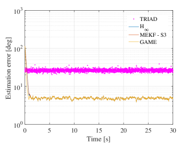
Figure 3: Measurement and estimation errors - RMS values (Case B)

Table 2: Estimation errors (deg) for Case B

	Transient	Steady state
	RMS error	RMS error
TRIAD	26.33	26.43
MEKF	14.82	4.84
$H_{\infty}$ Filter	14.63	4.85
GAME	11.85	4.84

The simulation results for this case are reported in Figure 3 and Table 2. We see that the GAME filter is still the winner during the transients, while the proposed $H_{\infty}$ filter is just a little better than the MEKF. At the steady-state, however, all the filters have comparable performance.

Remark 5.

It is a common practice that the filter gain is initialized with a sufficiently high numerical value which leads to faster convergence. It has been observed after several simulation runs that GAME filter, being a more agressive filter due to the geometric curvature correction terms, does not require such high numerical initialization. Instead, such a high gain initialization may even make GAME filter unstable in some extreme cases.

5 Conclusion

The problem of $H_{\infty}$ filtering on $SO(3)$ using vector directions has been investigated in this brief. A deterministic nonlinear $H_{\infty}$ filter has been derived which ensures that a dissipation inequality is satisfied for estimation errors up to $\pi/2$ radians, and that the energy gain from exogenous disturbances and estimation errors to a specified performance measure respects a given upper bound. The proposed filter has been compared with the quaternion MEKF, the quaternion $H_{\infty}$ filter, and the Geometric Approximate Minimum Energy (GAME) filter. The comparison suggests that the proposed filter can be viewed as a MEKF variant which can achieve better transient performance without significant degradation in steady-state performance. However, the approach used to obtain the filter has its limitations. In particular, the storage function considered can give, at best, only local stability and performance guarantees. In future work, we hope to re-visit the problem of worst-case $H_{\infty}$ estimation on $SO(3)$ using a chordal metric-based storage function, as well as to incorporate geometric curvature correction terms, such as those used in the GAME filter, in the gain update equation.

References

• [1] F. L. Markley, J. L. Crassidis, and Y. Cheng, “Nonlinear attitude filtering methods,” in AIAA Guidance, Navigation, and Control Conference, 2005, pp. 15–18.
• [2] J. L. Crassidis, F. L. Markley, and Y. Cheng, “Survey of nonlinear attitude estimation methods,” Journal of Guidance, Control, and Dynamics, vol. 30, no. 1, pp. 12–28, 2007.
• [3] A. J. van der Schaft, “$L_{2}$-gain analysis of nonlinear systems and nonlinear state-feedback $H_{\infty}$ control,” IEEE Transactions on Automatic Control, vol. 37, no. 6, pp. 770–784, 1992.
• [4] ——, “Nonlinear state space $H_{\infty}$ control theory,” in Essays on Control.   Springer, 1993, pp. 153–190.
• [5] A. Isidori, “$H_{\infty}$ control via measurement feedback for affine nonlinear systems,” International Journal of Robust and Nonlinear Control, vol. 4, no. 4, pp. 553–574, 1994.
• [6] A. Krener, “Necessary and sufficient conditions for nonlinear worst case ($H_{\infty}$) control and estimation,” Journal of Mathematical Systems, Estimation, and Control, vol. 4, no. 4, pp. 1–25, 1994.
• [7] N. Berman and U. Shaked, “$H_{\infty}$ nonlinear filtering,” International Journal of Robust and Nonlinear Control, vol. 6, no. 4, pp. 281–296, 1996.
• [8] A. P. Aguiar and J. P. Hespanha, “Robust filtering for deterministic systems with implicit outputs,” Systems & Control letters, vol. 58, no. 4, pp. 263–270, 2009.
• [9] F. Markley, N. Berman, and U. Shaked, “$H_{\infty}$-type filter for spacecraft attitude estimation,” Spaceflight Dynamics 1993, pp. 697–711, 1993.
• [10] ——, “Deterministic EKF-like estimator for spacecraft attitude estimation,” in American Control Conference, 1994, vol. 1.   IEEE, pp. 247–251.
• [11] L. Cooper, D. Choukroun, and N. Berman, Spacecraft Attitude Estimation via Stochastic $H_{\infty}$ Filtering.   American Institute of Aeronautics and Astronautics, 2010.
• [12] D. Choukroun, L. Cooper, and N. Berman, “Spacecraft attitude estimation and gyro calibration via stochastic $H_{\infty}$ filtering,” in Advances in Aerospace Guidance, Navigation and Control.   Springer, 2011, pp. 397–415.
• [13] N. A. Chaturvedi, A. K. Sanyal, and N. H. McClamroch, “Rigid-body attitude control,” IEEE Control Systems, vol. 31, no. 3, pp. 30–51, 2011.
• [14] R. Mahony, T. Hamel, and J.-M. Pflimlin, “Complementary filter design on the special orthogonal group SO(3),” in 44th IEEE Conference on Decision and Control, and European Control Conference. CDC-ECC’05.   IEEE, 2005, pp. 1477–1484.
• [15] ——, “Nonlinear complementary filters on the special orthogonal group,” IEEE Transactions on Automatic Control, vol. 53, no. 5, pp. 1203–1218, 2008.
• [16] S. Berkane and A. Tayebi, “On deterministic attitude observers on the Special Orthogonal group SO(3),” in 55th IEEE Conference on Decision and Control (CDC).   IEEE, 2016, pp. 1165–1170.
• [17] ——, “On the design of attitude complementary filters on $SO(3)$,” IEEE Transactions on Automatic Control, vol. 63, no. 3, pp. 880–887, 2017.
• [18] S. Bonnabel, P. Martin, and P. Rouchon, “Symmetry-preserving observers,” IEEE Transactions on Automatic Control, vol. 53, no. 11, pp. 2514–2526, 2008.
• [19] C. Lageman, J. Trumpf, and R. Mahony, “Gradient-like observers for invariant dynamics on a ${L}$ie group,” IEEE Transactions on Automatic Control, vol. 55, no. 2, pp. 367–377, 2010.
• [20] S. Bonnabel, P. Martin, and E. Salaün, “Invariant Extended Kalman Filter: theory and application to a velocity-aided attitude estimation problem,” in Proceedings of the 48th IEEE Conference on Decision and Control, 2009.   IEEE, 2009, pp. 1297–1304.
• [21] M. Zamani, J. Trumpf, and R. Mahony, “Near-optimal deterministic filtering on the rotation group,” IEEE Transactions on Automatic Control, vol. 56, no. 6, pp. 1411–1414, 2011.
• [22] ——, “A second order minimum-energy filter on the special orthogonal group,” in American Control Conference (ACC), 2012.   IEEE, 2012, pp. 1895–1900.
• [23] ——, “Minimum-energy filtering for attitude estimation,” IEEE Transactions on Automatic Control, vol. 58, no. 11, pp. 2917–2921, 2013.
• [24] M. Zamani, “Deterministic attitude and pose filtering, an embedded Lie groups approach,” Ph.D. dissertation, Australian National University, Canberra, Australia, 2013.
• [25] A. Saccon, J. Trumpf, R. Mahony, and A. P. Aguiar, “Second-order-optimal minimum-energy filters on ${L}$ie groups,” IEEE Transactions on Automatic Control, vol. 61, no. 10, pp. 2906–2919, 2016.
• [26] M. Zamani, J. Trumpf, and R. Mahony, “Nonlinear attitude filtering: a comparison study,” arXiv preprint arXiv:1502.03990, 2015.
• [27] M.-A. Lavoie, J. Arsenault, and J. R. Forbes, “An Invariant Extended $H_{\infty}$ Filter,” in 2019 IEEE 58th Conference on Decision and Control (CDC).   IEEE, 2019, pp. 7905–7910.
• [28] M. F. Haydar and M. Lovera, “$H_{\infty}$ filtering on the unit circle,” in 2017 IEEE 56th Annual Conference on Decision and Control (CDC).   IEEE, 2017, pp. 2422–2427.
• [29] F. L. Markley, “Multiplicative vs. additive filtering for spacecraft attitude determination,” Dynamics and Control of Systems and Structures in Space, pp. 467–474, 2004.
• [30] H. Gui and A. H. de Ruiter, “Quaternion invariant extended Kalman filtering for spacecraft attitude estimation,” Journal of Guidance, Control, and Dynamics, vol. 41, no. 4, pp. 863–878, 2018.
• [31] M. Izadi, E. Samiei, A. K. Sanyal, and V. Kumar, “Comparison of an attitude estimator based on the Lagrange-d’Alembert principle with some state-of-the-art filters,” in 2015 IEEE International Conference on Robotics and Automation (ICRA).   IEEE, 2015, pp. 2848–2853.
• [32] S. Berkane, “Hybrid attitude control and estimation on $SO(3)$,” Ph.D. dissertation, University of Western Ontario, London, Canada, 2017.
• [33] D. Simon, Optimal state estimation: Kalman, $H_{\infty}$, and nonlinear approaches.   John Wiley & Sons, 2006.
• [34] F. L. Lewis, L. Xie, and D. Popa, Optimal and robust estimation: with an introduction to stochastic control theory.   CRC press, 2007, vol. 29.