Linear Array Network for Low-light Image Enhancement

Abstract

Convolution neural networks (CNNs) based methods have dominated the low-light image enhancement tasks due to their outstanding performance. However, the convolution operation is based on a local sliding window mechanism, which is difficult to construct the long-range dependencies of the feature maps. Meanwhile, the self-attention based global relationship aggregation methods have been widely used in computer vision, but these methods are difficult to handle high-resolution images because of the high computational complexity. To solve this problem, this paper proposes a Linear Array Self-attention (LASA) mechanism, which uses only two 2-D feature encodings to construct 3-D global weights and then refines feature maps generated by convolution layers. Based on LASA, Linear Array Network (LAN) is proposed, which is superior to the existing state-of-the-art (SOTA) methods in both RGB and RAW based low-light enhancement tasks with a smaller amount of parameters. The code is released in https://github.com/cuiziteng/LASA_enhancement.

1 Introduction

Camera imaging system plays a fundamental role in modern artificial intelligence (AI) applications and human’s daily demand. However, images captured under low-light condition suffer from different kinds of degradation, such as undesired color distortion and in-camera noises. This would give an negative effect on human visual experience and downstream vision tasks, such as object detection  Cui et al. (2021), visual recognition Mao et al. (2021) and et al. There are mainly two sub-directions for recovering low-light images: one is mapping low-light RGB image to its’ normal-light RGB counterpart Lore et al. (2017); Wei et al. (2018), while another is to map low-light RAW measurements to normal-light RGB counterpart as an image signal processing (ISP) process Chen et al. (2018).

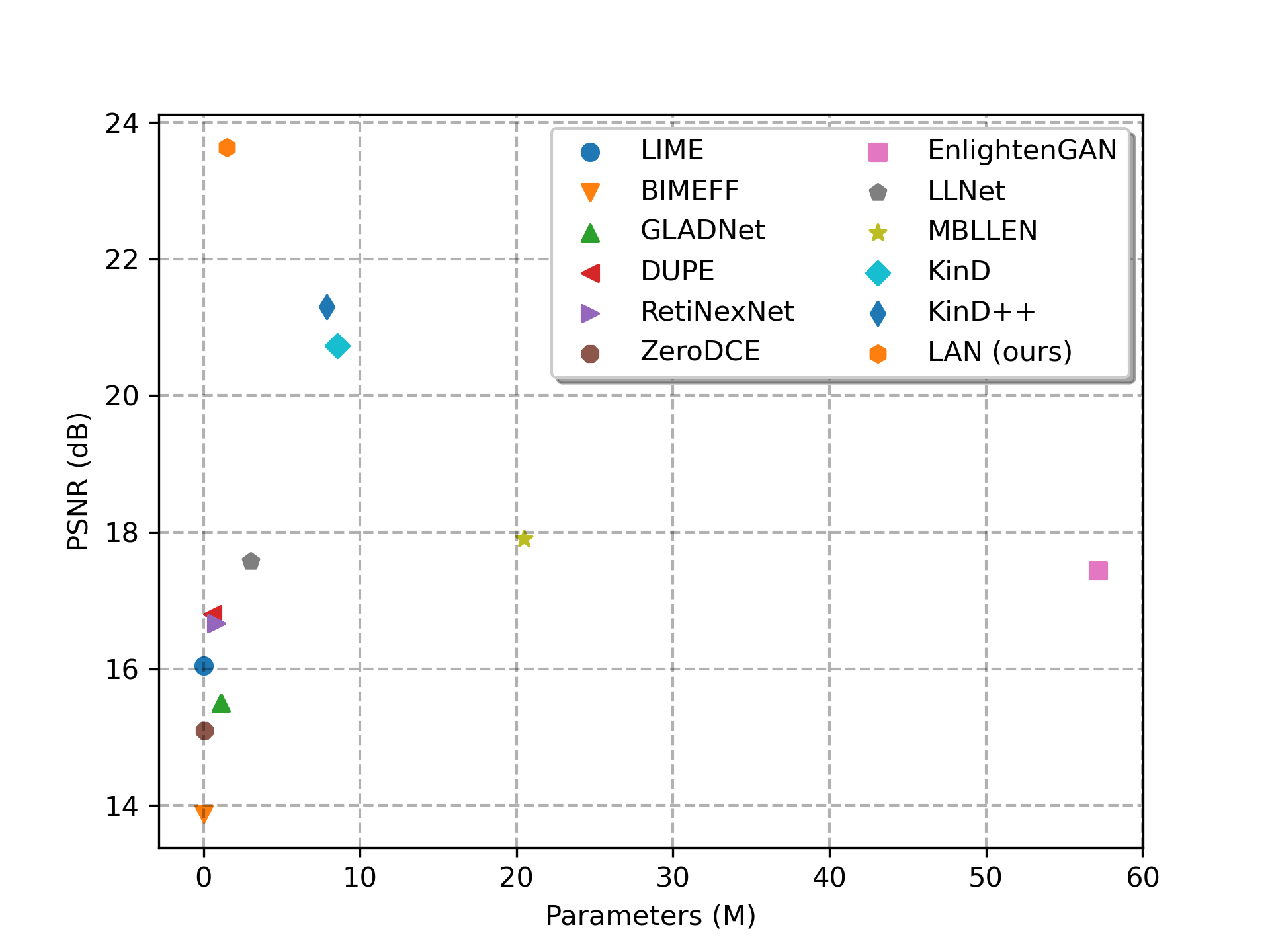
Figure 1: The best PSNR-parameter trade-off of LAN (ours).

In recent years, deep learning based methods have been dominant in the low-light image enhancement area and convolution neural network (CNN) plays a fundamental role in this task Lv et al. (2018); Chen et al. (2018); Wei et al. (2018); Zhang et al. (2019). It enables learning powerful feature representations via massively stacked convolution layers. To further boost the performance of convolution neural networks, a lot of efforts have been done on exploring more robust architectures. However, the inherent flaws of convolution neural networks (CNNs) have been always ignored. Specifically, CNNs are convolution operation based on a local sliding window mechanism, which only focuses on the local relations of feature maps within the sliding window and makes it difficult to construct the global representation directly.

Recently, transformer-based architectures have been widely used in visual tasks, which can effectively aggregate feature maps global information. However, visual transformer lacks the ability to constitute local feature representations, which is important for low-level visual tasks. Recent works  Gao et al. (2021); Peng et al. (2021) attempt to alleviate this problem by coupling the local feature maps and global representations. But the high computational cost of self-attention makes it difficult to cope with high resolution images directly even with the vast variants.

It is well known that attention mechanisms have been extensively used in previous literature, such as convolution block attention module (CBAM) Woo et al. (2018), SimAM Yang et al. (2021) and etc. A natural idea is, can we design an attention mechanism with 3-D global weights to refine CNNs feature maps instead of directly aggregating whole feature maps global relationship to reduce the computational cost? In light of this, this paper proposes a new attention mechanism named Linear Array Self-attention (LASA), which can directly infer 3-D global attention weights from current feature maps and then in turn refine these feature maps. The refined feature maps can implicitly couple the local and global relationships by adjusting the local feature maps using global weights. Specifically, LASA first encodes feature maps as two 2-D feature encodings along vertical and horizontal directions respectively. Then, the global representations are constructed using the self-attention mechanism. Finally, the 3-D global attention weights are generated by a multilayer perceptron (MLP) and a sigmoid activation function. By this means, we can reduce the computational cost of self-attention from $O((H\times W)^{2})$ to $O((H+W)^{2})$.

As shown in Fig. 1, this paper also develops a compact light-weight network named Linear Array Network (LAN) by adopting an autoencoder-like (AE) framework, which achieves the best trade-off between performance and the number of parameters compared with other methods. Our LAN is constructed by stacking multiple Linear Array Block (LAB), where LAB is composed of LASA and convolutional layers. Furthermore, multi-level features are also important for improving the performance of network. Therefore, LAN uses skip-connection (SC) and global residual learning (GRL) to fuse shallow and deep features. Our contributions can be summarized as:

(1) We propose a light-weight network for image restoration tasks and named Linear Array Network (LAN), which achieves SOTA results on both RGB and RAW based low-light image enhancement tasks and the best parameter-performance trade-off compared with other methods.

(2) Linear Array Self-attention (LASA) is proposed to enhance the global relationship construction ability of CNNs and handle the problem of the high computational complexity of self-attention.

(3) Extensive experiments prove that the validity of Linear Array Network (LAN) and Linear Array Self-attention (LASA). At the end, a series of ablation experiments are constructed to validate the rationality of each module in LAN.

2 Related Work

2.1 Low-light Image Enhancement

Modern low-light image enhancement tasks can be mainly split into two sub-directions: low-light RGB image enhancement and low-light RAW image reconstruction. For low-light RGB image enhancement, LLNet Lore et al. (2017) first introduce an auto-encoder like CNN structure to handle this task. Science then, various efforts have been done for using CNN-based structures Wei et al. (2018); Lv et al. (2018); Guo et al. (2020); Zhang et al. (2019); Jiang et al. (2021) to handle this task. RetiNexNet Wei et al. (2018) incorporate the RetiNex theory into CNN to let the network deal with the reflection part and illumination part separately, then combine them together to get the final output. Zero-DCE Guo et al. (2020) propose a self-supervised strategy which only uses low-light image for network training.

Low-light RAW image reconstruction can be seen as a more challenging task, since the unprocessed low-light raw data often contains different type of in-camera noises and color aberrations. Different from the traditional step-by-step methods for low-light RAW reconstruction, Chen et al. Chen et al. (2018) first propose a U-Net structure to handle this task, replacing the traditional manual-designed ISP pipeline, they also release the SID dataset which contains short-exposure low-light RAW images with their long-exposure RGB counterparts. In order to reduce the number of parameters of the model, some works Lamba et al. (2020); Gu et al. (2019) propose light-weight convolution neural networks (CNNs), however these methods reduce the quality of enhanced images at the same time. Our LAN could achieve SOTA performance on both two tasks and better parameter-performance trade-off compared with previous methods.

2.2 Attention Mechanism

Attention mechanisms are effective methods to boost the performance of CNNs via readjustment of feature maps, which enable CNNs to learn more reasonable information. Squeeze-and-Excitation (SE) attention learns the importance of different channels via learnable 1-D weights. However, SE attention ignores the spatial importance on the feature maps. To alleviate this problem, CBAM Woo et al. (2018) learns discriminative features by exploiting both spatial and channel-wise attention. In order to construct effective 3-D weights, SimAM Yang et al. (2021) combines neuroscience theories to propose a parameter-free attention module. Self-attention Vaswani et al. (2017) mechanism is an effective method to aggregate global information. However, it is proposed as an independent module which is hard to plug-and-play to CNNs, and the high computational cost makes it difficult to apply to high resolution images even with the vast variants. Different from the self-attention based methods that calculate the global relationship of the feature maps directly, inspired by the attention mechanisms used in CNNs, our LASA constructs the global relationship of feature maps implicitly through 3-D weights. To the best of our knowledge, LASA is the first work to introduce self-attention mechanism as an independent attention computing unit to low-light image enhancement tasks.

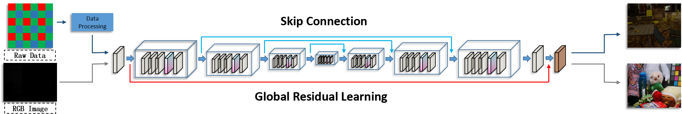
(a) Linear Array Network (LAN)

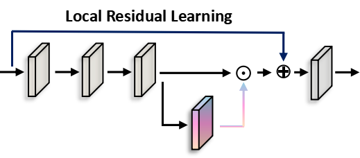
(b) Linear Array Block (LAB)

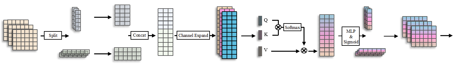
(c) Linear Array Self-attention (LASA)

Figure 2: Network architecture of the proposed Linear Array Network (LAN). Zoom in for best view.

3 Our Method

3.1 Pipeline

The current mainstream low-light image methods are mainly divided into two types, one is the method based on RGB images, and the other is the method of using RAW images to simulate image signal processor (ISP) . RGB images usually only contain 8-bit information, while RAW images have 12-bit or higher bits information. Therefore, RAW images are more suitable for low-light image enhancement, especially for extremely low-light environments. Since RAW image is unprocessed camera raw data, it needs to go through some data preprocessing operations before enhancement, such as black level correction and etc. The RAW image enhancement pipeline is used in this paper same as Chen et al. Chen et al. (2018), except that the image enhancement network is redesigned. For the enhancement pipeline of RGB images, this paper adopts an end-to-end approach like other low-light image enhancement methods based on RGB images.

3.2 Linear Array Network

To reduce the memory storage, Linear Array Network (LAN) is an autoencoder-like (AE) network. As show in Fig. 2, LAN mainly contains three parts: shallow feature extraction layers, linear array block (LAB), and finally the image restoration block. Our shallow feature extraction layers consists of one regular convolution layer, the extracted feature maps are used as input to the first LAB. In order to obtain global dense features from the original input image, shallow features are also combined with deep features through global residual learning (GRL). LAN also uses skip-connection (SC) to integrate the shallow (low-level features) and deep (high-level features) features with an addition operation. Each linear array block consists of four regular convolution layers, one linear array self-attention (LASA), and local residual learning (LRL). The linear array network uses seven linear array blocks, including three down-sampling modules and three up-sampling modules. The image restore block is composed of a regular convolutional layer and a sub-pixel layer Shi et al. (2016).

3.3 Linear Array Self-attention

The detailed structure of the Linear Array Self-attention (LASA) is shown in the Fig. 2. It can be seen as an independent computing unit to enhance the expressive power of convolutional neural networks, and can be integrated into any other network as a plug-and-play module. For a given feature map $\textbf{\emph{F}}~{}\in~{}\mathbb{R}~{}^{C\times H\times W}$, LASA can directly infer a 3-D weights $\textbf{\emph{F}}_{attention}~{}\in~{}\mathbb{R}~{}^{C\times H\times W}$ with global information to refine the feature map. The refined feature map can be computed as:

$$\textbf{\emph{F}}^{{}^{\prime}}=\textbf{\emph{F}}\cdot\textbf{\emph{F}}_{attention},$$ (1)

where $\cdot$ denotes element-wise multiplication, $C,H,W$ are the number of channels, height and width of feature maps F respectively. As for the LASA, we first encode feature map $\textbf{\emph{F}}~{}\in~{}\mathbb{R}~{}^{C\times H\times W}$ along the vertical and horizontal axes as a pair of 2-D feature encodings $\textbf{\emph{F}}_{x}~{}\in~{}\mathbb{R}~{}^{C\times 1\times W}$ and $\textbf{\emph{F}}_{y}~{}\in~{}\mathbb{R}~{}^{C\times H\times 1}$, which can be formulated as:

$$\textbf{\emph{F}}_{x}(i)=\frac{1}{H}\sum_{j=1}^{H}\textbf{\emph{F}}(i,j),$$ (2)

$$\textbf{\emph{F}}_{y}(j)=\frac{1}{W}\sum_{i=1}^{W}\textbf{\emph{F}}(i,j).$$ (3)

Next, we use matrix transformation operations to transform the sizes of feature map $\textbf{\emph{F}}_{x}~{}\in~{}\mathbb{R}~{}^{C\times W\times 1}$ and $\textbf{\emph{F}}_{y}~{}\in~{}\mathbb{R}~{}^{C\times 1\times H}$ into $\textbf{\emph{F}}_{x}~{}\in~{}\mathbb{R}~{}^{1\times C\times W}$ and $\textbf{\emph{F}}_{y}~{}\in~{}\mathbb{R}~{}^{1\times C\times H}$ respectively. We concat feature map $\textbf{\emph{F}}_{x}~{}\in~{}\mathbb{R}~{}^{1\times C\times W}$ and $\textbf{\emph{F}}_{y}~{}\in~{}\mathbb{R}~{}^{1\times C\times H}$ along channel dimension and get a new feature map $\textbf{\emph{F}}_{xy}~{}\in~{}\mathbb{R}~{}^{1\times C\times(H+W)}$. The number of channels of $\textbf{\emph{F}}_{xy}~{}\in~{}\mathbb{R}~{}^{1\times C\times(H+W)}$ will be expanded to three times of the original , and then divides it into three parts Q, K, and V in the channel dimension. Subsequently, the global relationship of the feature map is calculated, which can be formulated as:

$$\textbf{\emph{F}}_{global}=softmax(\textbf{\emph{Q}}\textbf{\emph{K}}^{\mathrm{\emph{T}}})\textbf{\emph{V}}+\textbf{\emph{F}}_{xy}.$$ (4)

As shown above, after calculating the global relationship of the feature map, we adopt the residual learning strategy to facilitate the gradient flow. At the end, the attention weights is computed as:

$$\textbf{\emph{F}}_{attention}=\sigma(MLP(\textbf{\emph{F}}_{global})).$$ (5)

where MLP is a multi-layer perceptron, $\sigma$ is a sigmoid function.

3.4 Loss Function

Given an input image $\textbf{\emph{I}}_{in}$ and a ground turth image $\textbf{\emph{I}}_{gt}$, the loss function $L_{mix}$ for LAN consists of L1 loss $L^{\ell_{1}}$, MS-SSIM Wang et al. (2003) loss $L_{MS-SSIM}$ and contrastive loss (CL) Wu et al. (2021) $L_{CL}$.

$$L^{\ell_{1}}=\frac{1}{N}\sum|\phi(\textbf{\emph{I}}_{in},w)-\textbf{\emph{I}}_{gt}|,$$ (6)

where $N$ is the number of the pixels.

where $M$ represents images of different scales, $\mu_{p}$ and $\mu_{g}$ represent the mean values of the predicted image and the ground truth image, $\sigma_{p}$ and $\sigma_{g}$ represents the standard deviation of the predicted image and the ground truth image, and $\sigma_{pg}$ is the covariance between the two images. $\alpha_{m}$ and $\beta_{m}$ represent the weight coefficients between the two items, and $c_{1}$ and $c_{2}$ are two constants.

$$L^{CL}_{i}=\frac{D(G_{i}(\phi(\textbf{\emph{I}}_{in},w)),G_{i}(\textbf{\emph{I}}_{gt}))}{D(G_{i}(\phi(\textbf{\emph{I}}_{in},w)),G_{i}(\textbf{\emph{I}}_{in}))},$$ (8)

where $D(x,y)$ is the $L_{1}$ distance, $L^{CL}_{i}$ is the $i$-th hidden features from the VGG model. Therefore, the overall loss function $L^{MIX}$ used for LAN can be formulated as:

$$L^{MIX}=\lambda_{1}\cdot L^{\ell_{1}}+\lambda_{2}\cdot L^{MS-SSIM}+\lambda_{3}\cdot\sum_{i}^{n}\cdot w_{i}\cdot L^{CL}_{i}.$$ (9)

where $\lambda_{1},\lambda_{2},\lambda_{3},w_{i}$ are the weight coefficients used to make trade-off for the importance of the loss function $L^{MIX}$.

4 Experiments and Results

(a) Input

(b) LTS

(c) LAN (Our)

(d) GT

Figure 3: Visual results comparison on SID dataset. Zoom in for best view.

LOL	PSNR (dB) $\uparrow$	SSIM $\uparrow$	GMSD $\downarrow$	NLPD $\downarrow$	NIQE $\downarrow$	DISTS $\downarrow$	Param $\downarrow$
LIME	16.0458	0.4834	0.1541	0.5129	10.8926	0.1806	-
BIMEF	13.8752	0.5936	0.0953	0.3645	9.8083	0.1878	-
GLADNet	15.5045	0.6247	0.2035	0.5169	16.9071	0.3072	1.128 M
DUPE	16.7975	0.5187	0.1675	0.5936	10.4406	0.1794	0.5652 M
RetiNexNet	16.6691	0.4909	0.1549	0.5799	8.9796	0.2450	0.838 M
ZeroDCE	15.0924	0.5093	0.1646	0.4878	10.4976	0.1891	0.0794 M
EnlightenGAN	17.4412	0.6744	0.1046	0.3674	14.8651	0.1638	57.17 M
LLNet	17.5777	0.6819	0.1485	0.4837	14.2112	0.2266	3.012 M
MBLLEN	17.9006	0.7020	0.1160	0.3447	14.7112	0.1448	20.4746 M
KinD	20.7261	0.8103	0.0888	0.3187	10.7841	0.1126	8.540 M
KinD++	21.3003	0.8226	0.0960	0.3174	11.3194	0.1169	7.8912 M
LAN (ours)	23.6324	0.8444	0.0670	0.2683	9.9427	0.0801	1.49 M

Table 1: Quantitative evaluation of low-light image enhancement algorithms on LOL dataset.The best results are highlighted in bold.

4.1 Experimental Setup

Dataset. Our evaluation experiments are constructed on two widely used low-light datasets: LOL dataset (RGB Images) and SID dataset (RAW Images). The LOL dataset contains 485 training samples and 15 testing samples. SID datasets consist of two sub-datasets: SID-Sony (SIDS) and SID-Fuji (SIDF). SIDS contains 231 high-exposure images and 2697 short-exposure images, and SIDF contains 193 high-exposure images and 2397 short-exposure images. Each high-exposure image corresponds to different short-exposure images in SIDS and SIDF.

Metrics. To evaluate the performance of our method, we have adopted the classical image quality assessment methods: Peak Signal to Noise Ratio (PSNR) and the Structural Similarity index (SSIM) as the evaluation metrics. They are usually used as the criteria to evaluate image quality in image restoration tasks. In order to conduct quantitative analysis objectively, we have also adopted other evaluation metrics, including PSNR, SSIM , gradient magnitude similarity deviation (GMSD) Xue et al. (2013), normalized Laplacian pyramid (NLPD) Laparra et al. (2016), natural image quality evaluator (NIQE) Mittal et al. (2012), deep image structure and texture similarity (DISTS) Ding et al. (2020).

Implementation Details. Our LAN is implemented by pytorch with one NVIDIA GeForce RTX 2080Ti GPU. The model is trained on Adam optimizer with default parameters. The epoch is set to 4000 and 2000 for SID and LOL, respectively. For these two datasets, we set the initial learning rate to 0.0001, and reduce the learning rate to one-tenth of the original in half of the training epoch. The batch size is set to 1 for both LOL and SID datasets. The data augmentation methods used during training are random rotation and flipping.

4.2 Quantitative Evaluation

We evaluate our method on two widely-adopted datasets, LOL and SID respectively. The compared methods on LOL dataset including LIME Guo et al. (2017), BIMEF Ying et al. (2017), GLADNet Wang et al. (2018), DUPE Wang et al. (2019), RetiNexNet Wei et al. (2018), ZeroDCE Guo et al. (2020), EnlightenGAN Jiang et al. (2021), LLNet Lore et al. (2017), MBLLEN Lv et al. (2018), KinD Zhang et al. (2019) and KinD++ Zhang et al. (2021). In addition, to evaluate the enhancement effectiveness of our proposed method, the models are also evaluated on extremely low-light dataset (SID). We compare our models with several state-of-the-art methods: LTS Chen et al. (2018), DID Maharjan et al. (2019), SGN Gu et al. (2019), LLPAckNet Lamba et al. (2020), EEMEFN Zhu et al. (2020), LDC Xu et al. (2020).

Tab. 1, Tab. 2 and Tab. 3 respectively reports quantitative results on LOL, SIDS and SIDF datasets. It can be seen that LAN achieves a better trade-off between model parameters and performance compared with other methods. From Tab. 1, we can find that LAN outperforms all the other competitors by a large margin under multiple evaluation metrics. As shown in Tab. 2 and Tab. 3, we can see that LAN also has great advantages compared to other methods in the RAW image based low-light image enhancement task. Although LAN has a slightly lower SSIM index than LDC by 0.06, the number of parameters of LDC is 5 times higher than that of LAN.

SIDS	PSNR (dB) $\uparrow$	SSIM $\uparrow$	Param $\downarrow$
LTS	28.88	0.787	7.7 M
DID	28.41	0.780	2.5 M
SGN	28.91	0.789	3.5 M
LLPAckNet	27.83	0.75	1.16 M
EEMEFN	29.60	0.795	40.713M
LDC	29.56	0.799	8.6 M
LAN (ours)	30.17	0.793	1.48 M

Table 2: Quantitative evaluation of low-light image enhancement algorithms on SIDS dataset.The best results are highlighted in bold.

SIDF	PSNR (dB) $\uparrow$	SSIM $\uparrow$	Param $\downarrow$
LTS	26.61	0.680	7.7 M
SCG	26.90	0.683	3.5 M
LLPackNet	24.13	0.59	1.16 M
EEMEFN	27.38	0.723	40.713M
LDC	26.70	0.681	8.6 M
LAN (ours)	28.02	0.720	1.49 M

Table 3: Quantitative evaluation of low-light image enhancement algorithms on SIDF dataset.The best results are highlighted in bold.

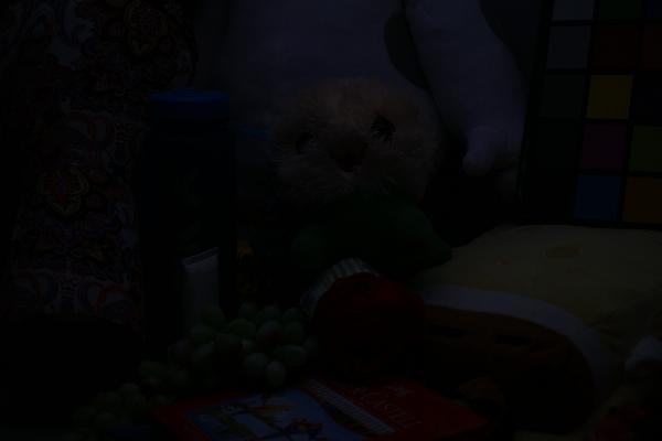
(a) Input

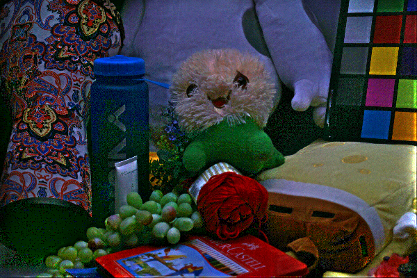
(b) LIME

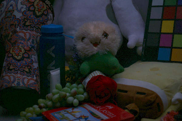
(c) BIMEF

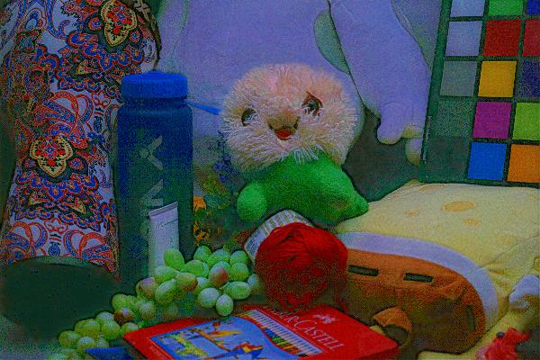
(d) RetinexNet

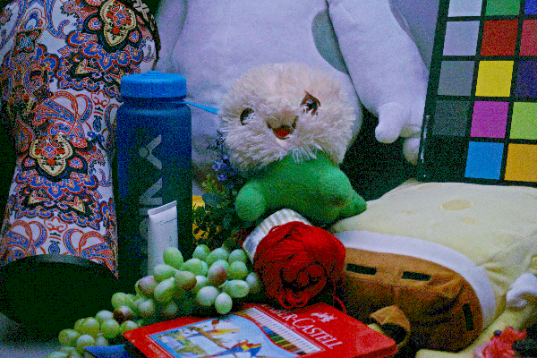
(e) ZeroDCE

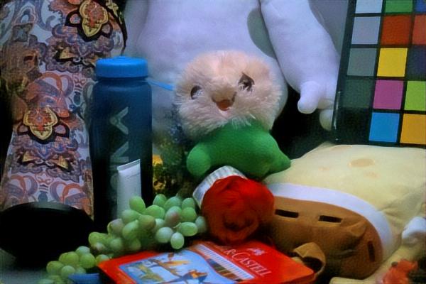
(f) MBLLEN

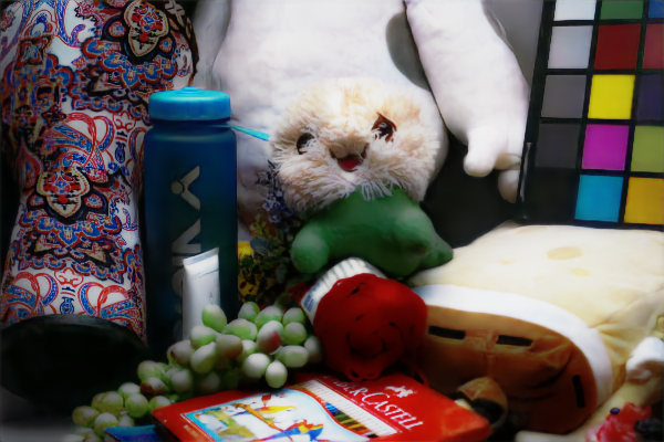
(g) KinD

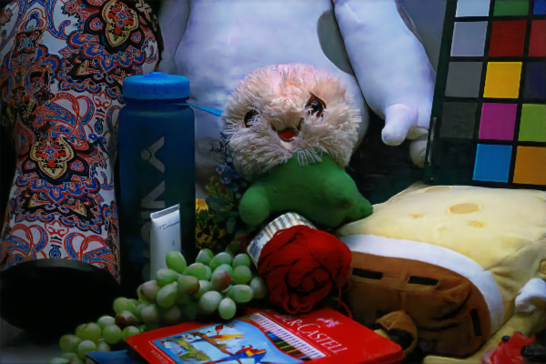
(h) KinD++

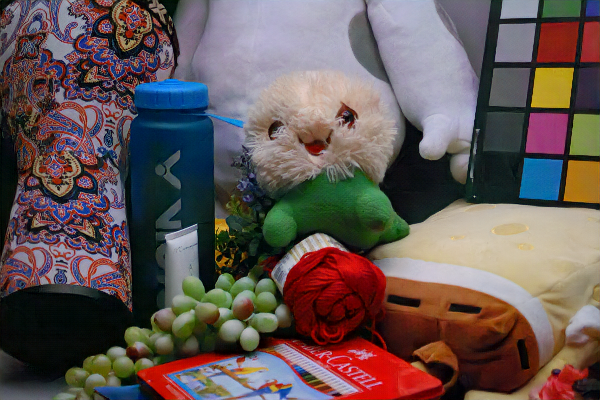
(i) LAN (Ours)

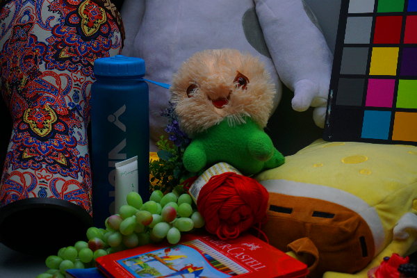
(j) GT

Figure 4: Visual results comparison on LOL dataset. Zoom in for best view.

Model	LASA	PSNR (dB) $\uparrow$	SSIM $\uparrow$
Base	-	15.485	0.569
Base+SC	-	28.702	0.784
Base+SC+GRL	-	28.907	0.785
Base+SC+GRL+LRL	-	28.673	0.784
Base+SC+GRL	$\surd$	30.075	0.794
Base+SC+GRL+LRL	$\surd$	30.170	0.793

Table 4: Ablation study on the design of Linear Array Network.

Model	Attention	PSNR (dB) $\uparrow$	SSIM $\uparrow$
LAN	-	28.673	0.784
LAN	CBAM	29.409 (0.736$\uparrow$)	0.784
LAN	SimAM	29.008 (0.335$\uparrow$)	0.785 (0.001$\uparrow$)
LAN	LASA	30.170 (1.497$\uparrow$)	0.793 (0.009$\uparrow$)
LTS	-	28.88	0.787
LTS	CBAM	27.334 (1.546$\downarrow$)	0.765 (0.022$\downarrow$)
LTS	SimAM	29.127 (0.247$\uparrow$)	0.785 (0.002$\downarrow$)
LTS	LASA	30.035 (1.155$\uparrow$)	0.792 (0.005$\uparrow$)

Table 5: Comparisons of different attention mechanism.

4.3 Qualitative Evaluation

We compare our approach with other methods on both SIDS and LOL datasets and provide the qualitative results in Fig. 3 and Fig. 4. As shown in Fig. 3, it is clear that our method have sharper details and more natural color constancy. Especially in the carton part of the picture, due to the ability to build global relationships, the color consistency is higher and no visual artifacts appear. From Fig. 4, we can see that compared with other methods, the enhanced image of LAN has lower noise, higher contrast, clearer texture details, and more realistic image content.

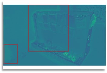
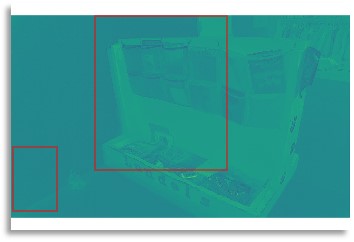
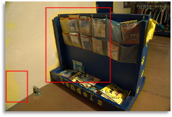
(a) CNNs

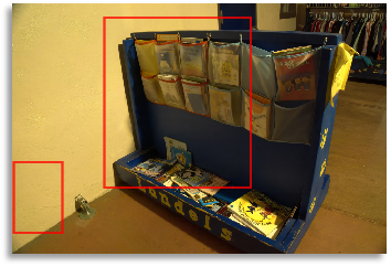
(b) CNNs+LASA

Figure 5: Visual comparison of with and without LASA.The upper part of the figure are the feature maps visualization results, and the lower part are the enhanced image results.

4.4 Ablation Experiment

In order to further verify the effectiveness of different elements on the network including skip-connection (SC), global residual learning (GRL), local residual learning (LRL) and LASA proposed in this paper, we constructed an ablation study. As shown in Tab. 4, the base network is the baseline of our ablation experiment, which mainly consists of three downsampling linear array blocks, three upsampling linear array blocks, one linear array block, shallow feature extraction layers and one image restoration block. In the LASA column of Tab. 4, ’-’ means LASA is not used, and ’$\surd$’ means LASA is used.

Subsequently, we gradually add different modules to the base network: (1) base+SC: Add the skip-connection (SC) operation into the baseline network. (2) base+SC+GRL: Add the skip-connection (SC) and the global residual learning (GRL) operation into the baseline network. (3) base+SC+GRL+LRL: Add the skip-connection (SC), gloabl residual learning (GRL) and local residual learning (LRL) operation into the baseline network. (4) base+SC+GRL+LASA: Add the skip-connection (SC), gloabl residual learning (GRL) and linear array self-attention into the baseline network. (5) base+SC+GRL+LRL+LASA: Add the skip-connection (SC), gloabl residual learning (GRL), local residual learning (LRL) and linear array self-attention into the baseline network. As we can see from Tab. 4, when we gradually add different modules to the baseline network, the performance of the model will gradually improve. Especially after using LASA, the PSNR will increase by more than 1 dB. Therefore, the effectiveness of the LASA can be fully proved.

Furthermore, to verify the effectiveness of LASA, we compared it with the commonly used 3-D wights attention mechanisms CBAM Woo et al. (2018) and SimAM Yang et al. (2021). As shown in the upper part of Tab. 5, using CBAM and SimAM in the LAN will bring a PSNR increase of 0.736 dB and 0.335 dB respectively, while using LASA will bring a PSNR increase of 1.497 dB. We also use the LTS Chen et al. (2018) as the baseline method for experimental comparison. From the bottom half of Tab. 5, we can see that the PSNR of LTS decreased by 1.546 dB after using CBAM. SimAM can increase the PSNR slightly by 0.247 dB and the PSNR goes up significantly by 1.155 dB when using LASA. Based on the experimental analysis above, LASA can be plugged into any network structure and therefore improves performance of network.

We also compare the performance of CNNs+LASA against using only CNNs, with LAN as the baseline network. As can be seen from Fig. 5, the method using only CNNs has a serious color imbalance problem, which can be effectively alleviated by using LASA.

5 Conclusion

In this paper, we propose Linear Array Network (LAN) for low-light image enhancement, which consists autoencoder-like (AE) network and Linear Array Self-attention (LASA). Our LAN has achieved SOTA results on both RAW based (SID) and RGB based (LOL) low-light image enhancement datasets with a small amount of parameters. The LASA attention mechanism proposed in this paper enables convolution operations to have the ability to establish long-range dependencies through refining feature maps, thereby improving the performance of convolution neural networks. A large number of comparative experiments and ablation experiments have verified the effectiveness of the proposed method. In future work, we will further explore the performance of this method on other image restoration tasks.

References

- Chen et al. [2018] C. Chen, Q. Chen, J. Xu, and V. Koltun. Learning to see in the dark. In CVPR, 2018.
- Cui et al. [2021] Ziteng Cui, Guo-Jun Qi, Lin Gu, Shaodi You, Zenghui Zhang, and Tatsuya Harada. Multitask aet with orthogonal tangent regularity for dark object detection. In ICCV, pages 2553–2562, October 2021.
- Ding et al. [2020] Keyan Ding, Kede Ma, Shiqi Wang, and Eero P Simoncelli. Image quality assessment: Unifying structure and texture similarity. arXiv preprint arXiv:2004.07728, 2020.
- Gao et al. [2021] Peng Gao, Jiasen Lu, Hongsheng Li, Roozbeh Mottaghi, and Aniruddha Kembhavi. Container: Context aggregation network. arXiv preprint arXiv:2106.01401, 2021.
- Gu et al. [2019] Shuhang Gu, Yawei Li, Luc Van Gool, and Radu Timofte. Self-guided network for fast image denoising. In ICCV, pages 2511–2520, 2019.
- Guo et al. [2017] Xiaojie Guo, Yu Li, and Haibin Ling. Lime: Low-light image enhancement via illumination map estimation. IEEE TIP, 26(2):982–993, 2017.
- Guo et al. [2020] C. Guo, C. Li, J. Guo, C. C. Loy, J. Hou, S. Kwong, and R. Cong. Zero-reference deep curve estimation for low-light image enhancement. In CVPR, pages 1777–1786, 2020.
- Jiang et al. [2021] Yifan Jiang, Xinyu Gong, Ding Liu, Yu Cheng, Chen Fang, Xiaohui Shen, Jianchao Yang, Pan Zhou, and Zhangyang Wang. Enlightengan: Deep light enhancement without paired supervision. IEEE TIP, 30:2340–2349, 2021.
- Lamba et al. [2020] Mohit Lamba, Atul Balaji, and Kaushik Mitra. Towards fast and light-weight restoration of dark images. arXiv preprint arXiv:2011.14133, 2020.
- Laparra et al. [2016] Valero Laparra, Johannes Ballé, Alexander Berardino, and Eero P Simoncelli. Perceptual image quality assessment using a normalized laplacian pyramid. Electronic Imaging, 2016(16):1–6, 2016.
- Lore et al. [2017] Kin Gwn Lore, Adedotun Akintayo, and Soumik Sarkar. Llnet: A deep autoencoder approach to natural low-light image enhancement. Pattern Recognition, 61:650 – 662, 2017.
- Lv et al. [2018] Feifan Lv, Feng Lu, Jianhua Wu, and Chongsoon Lim. Mbllen: Low-light image/video enhancement using cnns. In BMVC, 2018.
- Maharjan et al. [2019] Paras Maharjan, Li Li, Zhu Li, Ning Xu, Chongyang Ma, and Yue Li. Improving extreme low-light image denoising via residual learning. In ICME, pages 916–921. IEEE, 2019.
- Mao et al. [2021] Mingyuan Mao, Renrui Zhang, Honghui Zheng, Peng Gao, Teli Ma, Yan Peng, Errui Ding, and Shumin Han. Dual-stream network for visual recognition. arXiv preprint arXiv:2105.14734, 2021.
- Mittal et al. [2012] Anish Mittal, Rajiv Soundararajan, and Alan C Bovik. Making a ”completely blind” image quality analyzer. IEEE Signal processing letters, 20(3):209–212, 2012.
- Peng et al. [2021] Zhiliang Peng, Wei Huang, Shanzhi Gu, Lingxi Xie, Yaowei Wang, Jianbin Jiao, and Qixiang Ye. Conformer: Local features coupling global representations for visual recognition. CoRR, abs/2105.03889, 2021.
- Shi et al. [2016] Wenzhe Shi, Jose Caballero, Ferenc Huszar, Johannes Totz, Andrew P. Aitken, Rob Bishop, Daniel Rueckert, and Zehan Wang. Real-time single image and video super-resolution using an efficient sub-pixel convolutional neural network. In CVPR, pages 1874–1883, 2016.
- Vaswani et al. [2017] Ashish Vaswani, Noam Shazeer, Niki Parmar, Jakob Uszkoreit, Llion Jones, Aidan N. Gomez, Łukasz Kaiser, and Illia Polosukhin. Attention is all you need. Red Hook, NY, USA, 2017. Curran Associates Inc.
- Wang et al. [2003] Z. Wang, E.P. Simoncelli, and A.C. Bovik. Multiscale structural similarity for image quality assessment. In The Thrity-Seventh Asilomar Conference on Signals, Systems Computers, 2003, volume 2, pages 1398–1402 Vol.2, 2003.
- Wang et al. [2018] W. Wang, C. Wei, W. Yang, and J. Liu. Gladnet: Low-light enhancement network with global awareness. In 2018 13th IEEE International Conference on Automatic Face Gesture Recognition (FG 2018), pages 751–755, 2018.
- Wang et al. [2019] Ruixing Wang, Qing Zhang, Chi-Wing Fu, Xiaoyong Shen, Wei-Shi Zheng, and Jiaya Jia. Underexposed photo enhancement using deep illumination estimation. In CVPR, pages 6849–6857, 2019.
- Wei et al. [2018] Chen Wei, Wenjing Wang, Wenhan Yang, and Jiaying Liu. Deep retinex decomposition for low-light enhancement. In BMVC, 2018.
- Woo et al. [2018] Sanghyun Woo, Jongchan Park, Joon-Young Lee, and In So Kweon. CBAM: convolutional block attention module. In ECCV, 2018.
- Wu et al. [2021] Haiyan Wu, Yanyun Qu, Shaohui Lin, Jian Zhou, Ruizhi Qiao, Zhizhong Zhang, Yuan Xie, and Lizhuang Ma. Contrastive learning for compact single image dehazing. In CVPR, pages 10551–10560, 2021.
- Xu et al. [2020] Ke Xu, Xin Yang, Baocai Yin, and Rynson W.H. Lau. Learning to restore low-light images via decomposition-and-enhancement. In CVPR, June 2020.
- Xue et al. [2013] Wufeng Xue, Lei Zhang, Xuanqin Mou, and Alan C Bovik. Gradient magnitude similarity deviation: A highly efficient perceptual image quality index. IEEE TIP, 23(2):684–695, 2013.
- Yang et al. [2021] Lingxiao Yang, Ru-Yuan Zhang, Lida Li, and Xiaohua Xie. Simam: A simple, parameter-free attention module for convolutional neural networks. In ICML, 2021.
- Ying et al. [2017] Zhenqiang Ying, Ge Li, and Wen Gao. A bio-inspired multi-exposure fusion framework for low-light image enhancement. arXiv preprint arXiv:1711.00591, 2017.
- Zhang et al. [2019] Yonghua Zhang, Jiawan Zhang, and Xiaojie Guo. Kindling the darkness: A practical low-light image enhancer. MM ’19, New York, NY, USA, 2019. Association for Computing Machinery.
- Zhang et al. [2021] Yonghua Zhang, Xiaojie Guo, Jiayi Ma, Wei Liu, and Jiawan Zhang. Beyond brightening low-light images. International Journal of Computer Vision, 129(4):1013–1037, 2021.
- Zhu et al. [2020] Minfeng Zhu, Pingbo Pan, Wei Chen, and Yi Yang. Eemefn: Low-light image enhancement via edge-enhanced multi-exposure fusion network. In AAAI, volume 34, pages 13106–13113, 2020.