Information causality beyond the random access code model

Abstract

Information causality (IC) was one of the first principles that have been invoked to bound the set of quantum correlations. For some families of correlations, this principle recovers exactly the boundary of the quantum set; for others, there is still a gap. We close some of these gaps using a new quantifier for IC, based on the notion of “redundant information”. The new definition is still obeyed by quantum correlations. This progress was made possible by the recognition that the principle of IC can be captured without referring to the success criterion of random access codes.

I Introduction

Quantum theory differs from classical theory by the fact that the space of states is a vector space, rather than a set. This change has been necessary to accommodate the fact that only a fraction of the possible physical properties can be well-defined in any given state. But why a vector space, instead of something else? The basic answer is pragmatic: it has worked amazingly well. But of course, it would be desirable to know which principles underlie this choice. In the last decades, it was understood that quantum entanglement plays a crucial role in addressing this question. All the recent representation theorems use an axiom that has to do with composite systems (see D’Ariano et al. (2017) for an overview).

The most direct signature of entanglement are the quantum correlations obtained by measuring the sub-systems separately. It is well known that some of these correlations cannot be reproduced within classical theory without communication, because they violate Bell’s inequalities Scarani (2019). Instead of recovering the whole of quantum theory, a series of works have tried to find principles that single out the set $\mathcal{Q}$ of quantum correlations (save the phenomena, rather than the whole formalism). Since measurements on shared entanglement cannot be used to send a signal, Popescu and Rohrlich asked whether this no-signaling principle singles out quantum correlations exactly: they quickly found that it does not Popescu and Rohrlich (1994). The question then became: can one find other principles, to add on top of no-signaling, so as to identify the set $\mathcal{Q}$?

Several such principles were proposed Brassard et al. (2006); Pawłowski et al. (2009); Navascués and Wunderlich (2010); Fritz et al. (2013). Most of them have later been proved to be satisfied in the set of “almost-quantum” correlations Navascués et al. (2015), which is strictly larger than $\mathcal{Q}$. Thus, those principles are satisfied by all quantum correlations, but they don’t identify $\mathcal{Q}$. For the principle of information causality (IC) Pawłowski et al. (2009), our knowledge is less definite. For sure, all quantum correlations satisfy it; but its relations with the set of almost-quantum correlations is not known, and it is then still possible that IC identifies $\mathcal{Q}$ for bipartite Bell correlations (some modifications will be needed for multipartite ones Gallego et al. (2011); Yang et al. (2012)). IC was defined in terms of a task: a classical random access code (RAC), augmented by sharing the no-signaling resource under study between the two players. In this paper, we propose to redefine IC in a way that captures the same underlying notion as the original, but without reference to the specific task of RAC. The new criterion is still obeyed by all quantum correlations, but is violated by a larger set of non-quantum correlations. To substantiate this claim, we show the first tightening of the IC boundary in the simplest Bell scenario (two parties, two inputs and two outputs, 2-2-2) since the original study Allcock et al. (2009).

II Redefining information causality

We use upper case letters $A,B$ to denote random variables, lower case letters $a,b$ to denote specific values. For bits, thus, one should understand $A=\{0,1\}$, and then $a=0$ or $a=1$. The probability distribution of the variable $X$ is denoted $p_{X}$, with $p_{X}(x)$ the probability of its event $x$ (we may sometimes omit the subscript for simplicity).

To define IC, one considers the following two-player game. At every round, Alice’s input is a string of $N$ bits $A=A_{1}\times...\times A_{N}$, its value $a=(a_{1},...,a_{N})$ drawn at random with uniform distribution. She can send information to Bob on a channel with capacity $k$ per round. In addition, she shares a no-signaling resource with Bob. If $k<N$, Bob obviously can retrieve at most $k$ bits of Alice’ input, irrespective of what the no-signaling resource is. But with a clever use of some no-signaling resources, something unexpected may happen: Bob could choose which $k$ bits to retrieve. In words, it looks like the information about all $N$ bits was “potentially” present at Bob’s location, although eventually he can read out only $k$ of them. The principle of IC states that this should not happen; and more quantitatively: even the “potential information” available at Bob’s location should not exceed the capacity $k$ of the channel linking Alice and Bob. In this paper we discuss how this potential information should be quantified.

In the original paper Pawłowski et al. (2009) and all subsequent works Allcock et al. (2009); Barnum et al. (2010); Cavalcanti et al. (2010); Al-Safi and Short (2011); Yang et al. (2012); Miklin and Pawłowski (2021), IC was captured by a random access code (RAC) criterion: Bob receives an input $t\in\{1,...,N\}$ that tells him which of Alice’s bits he is supposed to retrieve in any given round. Over many rounds, then, the potential information is estimated by

$$IC_{\textrm{RAC}}=\sum_{i=1}^{N}I(A_{i};B|t=i)\,\equiv\,\sum_{i=1}^{N}I(A_{i};B_{i})\,.$$ (1)

With this criterion, IC is satisfied if

$$IC_{\textrm{RAC}}\leq k.$$ (2)

The intuition behind such RAC type of IC characterization is: we would find it surprising if, in every round, Bob could produce the correct value $b_{i}=a_{i}$ for the requested $i$, thus achieving $IC_{\textrm{RAC}}=N$.

But the definition of potential information does not necessarily require a game with a specific winning criterion for each round. The input $A$ of Alice can be treated as a single symbol (which doesn’t even need to have the dimension of a string of bits), and the number $M$ of Bob’s inputs can be an independent number (even if Alice’s input were $N$ bits, we could have $M\neq N$). After many rounds, Alice and Bob can estimate the $M$ probability distributions $p_{AB}(a,b|t=i)\equiv p_{AB_{i}}(a,b_{i})$. A bound on potential information can be obtained directly from those. Specifically, the quantifier of potential information that we consider would read

$$IC_{\textrm{red}}(M)=\sum_{i=1}^{M}I(A;B_{i})-I_{r}(A;B_{1},...,B_{M})\,.$$ (3)

The first term in (3) is the sum of the mutual information of $A$ with each of the $B_{i}$. It can easily reach $Mk$ if $B_{1}$ carries all the information $k$, and all the other $B_{i}$ are set equal to $B_{1}$ and thus carry the same piece of information. This observation is the basis for understanding the role of the second term: one needs to remove redundant information, i.e. information that is present in several $B_{i}$. The characterization of redundant information is still debated. The lack of a general expression for $I_{r}(A;B_{1},...,B_{M})$ is the current limit for our study of IC. Fortunately, the interest of the approach can already be proved in the simplest case $M=2$, for which an expression for redundant information has been given.

III IC with Redundant Information

We are going to study

$$IC_{\textrm{red}}=\sum_{i=1}^{2}I(A;B_{i})-I_{r}(A;B_{1},B_{2})$$ (4)

with the measure of redundant information proposed by Harder, Salge and Polani Harder et al. (2013). We first describe this measure, then prove that quantum correlations obey IC with our new definition, that is

$$IC_{\textrm{red}}\leq k\,.$$ (5)

III.1 The measure of redundant information

Let us now give the recipe of Ref. Harder et al. (2013) to compute redundant information. The starting point are the two joint probability distributions $p_{AB_{i}}$ for $i=1,2$. From $p_{AB_{i}}$, for each value of $B_{i}$ one constructs the probability distribution $p_{A|b_{i}}$ on $A$. These are $|B_{i}|$ points in the probability simplex of $A$, and we denote by $C_{i}$ their convex hull. For $|B|=2$, as is the case for us,

$$C_{i}=\big{\{}\lambda p_{A|b_{i}=0}+(1-\lambda)p_{A|b_{i}=1}\,|\,\lambda\in[0,1]\big{\}}\,.$$ (6)

Now, for every value $b_{1}$ of $B_{1}$, one defines $p_{A[b_{1}\searrow B_{2}]}$ as the element of $C_{2}$ that is “closest” to $p_{A|b_{1}}$ in the following sense:

$$p_{A[b_{1}\searrow B_{2}]}:=\textrm{argmin}_{r\in C_{2}}D_{KL}(p_{A|b_{1}}||r),$$ (7)

where $D_{KL}$ is the Kullback-Leibler divergence. Having solved this optimisation for all $b_{1}$, one can compute the “projected information”

$$I_{A}^{\pi}(B_{1}\searrow{B_{2}})=\sum_{a,b_{1}}p_{AB_{1}}(a,b_{1})\log\left(\frac{p_{A[b_{1}\searrow B_{2}]}(a)}{p_{A}(a)}\right)\,.$$ (8)

After repeating the recipe with $B_{1}$ and $B_{2}$ exchanged, redundant information is finally computed as

$$I_{r}(A;B_{1},B_{2}):=\min\{I_{A}^{\pi}(B_{1}\searrow B_{2}),I_{A}^{\pi}(B_{2}\searrow B_{1})\}\,.$$ (9)

Among the properties of $I_{r}$, it was proved in Harder et al. (2013) that the quantity (4) is bounded as $IC_{\textrm{red}}\leq I(A;B_{1},B_{2})$. Notice that $I_{r}$, and thence $IC_{\textrm{red}}$, is a functional of the two marginal distributions $p_{AB_{i}}$ only. Thus, explicitly, the bound just mentioned reads

$$IC_{\textrm{red}}[p_{AB_{1}},p_{AB_{2}}] \leq I(A;B_{1},B_{2})[p_{AB_{1}B_{2}}]$$ (10)

and holds for every joint probability distribution $p_{AB_{1}B_{2}}$ that has marginals $p_{AB_{1}},p_{AB_{2}}$. We are going to use this observation to prove that IC holds for quantum correlations.

III.2 Proof that IC holds for quantum correlations

When the shared no-signaling resource is quantum, Bob’s outputs $B_{i}$ are generated by processing the information available to him. This consists of his part $\rho_{B}=\textrm{Tr}_{A}(\rho_{AB})$ of the initially shared state $\rho_{AB}$, and of the classical message $m$ received by Alice. We denote this variable by $Q_{Bm}$ and its set of events by $\{\rho_{Bm}\}$. The observed quantum correlations will be given by

$$p_{AB_{i}}(a,b_{i})\equiv\sum_{\rho_{Bm}}p(\rho_{Bm})p(a,b_{i}|\rho_{Bm})\,.$$ (11)

But crucially, the information about $A$ in $B_{i}$ is mediated by $Q_{Bm}$, i.e. we have a Markov chain $A\rightarrow Q_{Bm}\rightarrow B_{i}$. Therefore

$$p(a,b_{i}|\rho_{Bm})=p(a|\rho_{Bm})p(b_{i}|\rho_{Bm})$$ (12)

holds for every $\rho_{Bm}$. Then we can construct the joint distribution

$$p_{AB_{1}B_{2}}(a,b_{1},b_{2})\equiv$$ (13)

$$\sum_{\rho_{Bm}}p(\rho_{Bm})p(a|\rho_{Bm}) p(b_{1}|\rho_{Bm})p(b_{2}|\rho_{Bm})$$ (14)

whose marginals with respect to either of the $B_{i}$ are indeed the quantum correlations (11). For this distribution, the data-processing inequality gives

$$I(A;B_{1},B_{2})[p_{AB_{1}B_{2}}]\leq I(A;Q_{Bm})\,.$$ (15)

Finally, $I(A;Q_{Bm})\leq k$ is just another application of the same inequality, capturing the fact that only the message $m$ has carried information about $A$ to Bob, and shared quantum information does not change that (see the formal proof in the first paper on IC Pawłowski et al. (2009)). By comparison with (10), we have proved that IC holds for shared quantum resources according to our new definition Eq. (5).

IV Evidence of improvement

We now prove that our approach to IC constitutes a real improvement over the original one, as it rules out more non-quantum correlations. Specifically, we are going to report the first improvement on IC for the 2-2-2 scenario since the original study by Allcock and coworkers Allcock et al. (2009).

IV.1 Definitions and protocol

We denote $x,y\in\{0,1\}$ the inputs to the boxes, $\mathfrak{a},\mathfrak{b}\in\{0,1\}$ the outputs. The set of no-signaling correlation is a polytope with 24 vertices: 8 extremal non-local boxes, which can be parametrized by $\mu,\nu,\sigma\in\{0,1\}$ as

$$P_{NL}^{\mu\nu\sigma}(\mathfrak{a}\mathfrak{b}|xy)=\left\{\begin{array}[]{ll}\frac{1}{2},&\textrm{if}\ \mathfrak{a}\oplus\mathfrak{b}=xy\oplus\mu x\oplus\nu y\oplus\sigma\\ 0,&\textrm{otherwise}\,;\end{array}\right.$$ (16)

and 16 local deterministic boxes, which can be parametrized by $\mu,\nu,\sigma,\tau\in\{0,1\}$ as

$$P_{L}^{\mu\nu\sigma\tau}(\mathfrak{a}\mathfrak{b}|xy)=\left\{\begin{array}[]{ll}1,&\textrm{if}\ \mathfrak{a}=\mu x\oplus\nu,\ \mathfrak{b}=\sigma y\oplus\tau\\ 0,&\textrm{otherwise}.\end{array}\right.$$ (17)

The box $P_{NL}^{000}$ is the canonical form of the PR-box, maximizing the value of $CHSH=C_{00}+C_{01}+C_{10}-C_{11}$ where $C_{xy}=P(\mathfrak{a}=\mathfrak{b}|xy)-P(\mathfrak{a}\neq\mathfrak{b}|xy)$. All the other $P_{NL}^{\mu\nu\sigma}$ are obtained from it by relabelling some of the inputs and/or some of the outputs, and maximize the corresponding CHSH-type expression.

No method is known to decide whether a no-signaling resource violates IC based on the description of the box alone: one needs to invent an explicit protocol that uses that resource (the fact that this protocol may not be optimal is the main reasons why the exact boundaries of the violation of IC are not known). Here, we follow a recently proposed compact protocol Miklin and Pawłowski (2021). Although it led to some improvements for other scenarios, for the 2-2-2 scenario this protocol reproduced the results of Allcock et al. (2009). Thus, the improvement we are going to report is really due to our new definition of IC.

The protocol is the following. Alice inputs $x=a_{1}\oplus a_{2}$ into the box; upon receiving the output $\mathfrak{a}$, she computes the bit $m=\mathfrak{a}\oplus a_{1}$. She sends this bit to Bob on a noisy channel: specifically, a symmetric binary channel that flips the bit with probability $1-p_{c}$. The capacity of this channel is

$$k=1+p_{c}\log_{2}p_{c}+(1-p_{c})\log_{2}(1-p_{c})\,.$$ (18)

The bounds for IC get tighter in the limit $p_{c}\rightarrow\frac{1}{2}$ Miklin and Pawłowski (2021).

On his side, when Bob wants to estimate $B_{i}$, he inputs $y=i-1$ in the box. Upon receiving the output $\mathfrak{b}$, he produces $b_{i}=\mathfrak{b}\oplus m^{\prime}$ where $m^{\prime}$ is the output of the noisy channel from Alice.

IV.2 Case studies

As concrete case studies, we look at the same three families of boxes studied in Allcock et al. (2009). These families are defined by the convex combination

$$PR_{\alpha,\beta}=\alpha P_{NL}^{000}+\beta R_{NS}+(1-\alpha-\beta)\mathbb{I},$$ (19)

where $\alpha\in[0,1]$, $\beta\in[0,1-\alpha]$, $R_{NS}$ is an extremal point of the no-signaling polytope, and $\mathbb{I}$ indicates the white noise $P(\mathfrak{a}\mathfrak{b}|xy)=\frac{1}{4}$. The case studies will involve the same three choices of $R_{NS}$ as Allcock et al. (2009), namely $P_{NL}^{010}$, $P_{NL}^{110}$ and $P_{L}^{0000}$. By the symmetry of the problem, this choice covers actually all cases: $P_{NL}^{010}$ is equivalently to $P_{NL}^{011}$, $P_{NL}^{100}$, and $P_{NL}^{101}$; $P_{NL}^{110}$ is equivalent to $P_{NL}^{111}$; and all the local deterministic points on the facet $CHSH=2$ are equivalent. Finally, since $P_{NL}^{001}=2\mathbb{I}-P_{NL}^{000}$ is the PR-box opposite to the canonical one, that mixing is already taken into account in (19).

The explicit expressions needed to compute the $p_{AB_{i}}$ for each case are given in Table 1. The numerical calculations require setting $p_{c}$ close to $\frac{1}{2}$ because the tightest bounds are found in that limit Miklin and Pawłowski (2021); and identifying the minimum in (7). These are reliably dealt with by sampling evenly and by varying some precision parameters, details are given in footnote . As a check, we also redid the curves for the original IC criterion and recovered the plots of Allcock et al. (2009) as expected.

The results are shown graphically in Fig. 1. In summary:

• For $R_{NS}=P_{NL}^{010}$ (or $P_{NL}^{011}$, $P_{NL}^{100}$, $P_{NL}^{101}$), both the original definition of IC and our new one recover the boundary of the quantum set (within numerical precision).

• $R_{NS}=P_{NL}^{110}$ (or $P_{NL}^{111}$), the original definition of IC stayed very far from the quantum boundary: in fact, it could just detect a violation of IC for those boxes that violate the Tsirelson bound. By contrast, our new definition recovers exactly the quantum set, within numerical precision.

• Finally, for $R_{NS}=P_{L}^{0000}$ (or any other local deterministic point on the facet $CHSH=2$), our definition and the original one give the same boundary for IC, but there remains a gap with the quantum boundary.

The fact that the original definition recovered the quantum boundary for some $R_{NS}=P_{NL}^{\mu\nu\sigma}$ but not others was an artefact of the use of RAC. This can be intuited by looking at the behavior of the extremal points for $p_{c}=1$. For the canonical PR-box $P_{NL}^{000}$, the protocol yields $A_{1}=B_{1}$ and $A_{2}=B_{2}$; for $R_{NS}=P_{NL}^{110}$, the same protocol yields $A_{1}=B_{2}\oplus 1$ and $A_{2}=B_{1}$. The amount of potential information is the same for both points (each $B_{i}$ has full information on one of the $A_{j}$), and our definition captures this. Imposing the RAC winning condition $A_{i}=B_{i}$ breaks the symmetry.

When $R_{NS}=P_{L}^{0000}$, the quantum boundary is provably a straight line Goh et al. (2018). The boundary of the set of “almost-quantum” correlations $\mathcal{Q}_{1+AB}$ is indistinguishable from it at the scale of the figure . A significant gap remains between those sets and the violation of IC, even with the new definition that here does not improve on the original one. This gap may be real: definitely, this is a slice where one could focus the efforts to prove that IC does not coincide with $\mathcal{Q}$. Alternatively, we may not have captured “potential information” at its tightest yet. For instance, Ref. Ince (2017) argues that redundant information may have to depend also on the joint distribution of Bob’s outputs $p_{B_{1}B_{2}}$ and not just on the marginals with Alice $p_{AB_{i}}$.

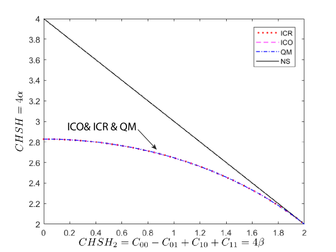
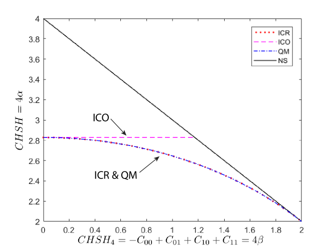
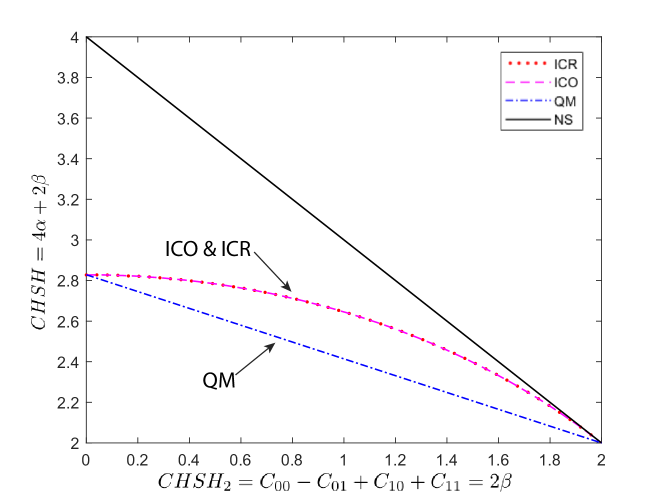
Figure 1: Slices (19) of the non-signalling polytope studied in this work: from top to bottom, $R_{NS}=P_{NL}^{010}$, $R_{NS}=P_{NL}^{110}$, and $R_{NS}=P_{L}^{0000}$. In all figures, the top left corner is the PR box $P_{NL}^{000}$, the bottom line is the facet $CHSH=2$. ICO represents IC for the original definition (2); these are the curves found in Allcock et al. (2009). ICR represents IC for our definition based on redundant information (5). The quantum boundary is the Tsirelson-Landau-Masanes bound (see Scarani (2019)) for the first two figures, and a straight line for the third Goh et al. (2018).

$R_{NS}$	$P^{010}_{NL}$		$P^{110}_{NL}$		$P^{0000}_{L}$
	$B_{1}$	$B_{2}$	$B_{1}$	$B_{2}$	$B_{1}$	$B_{2}$
$a=00$	$k_{+}$	$k_{-}$	$k_{+}$	$k_{-}$	$k_{+}$	$k_{+}$
$a=01$	$k_{+}$	$1-k_{-}$	$k_{-}$	$1-k_{+}$	$k_{+}$	$1-k_{-}$
$a=10$	$1-k_{+}$	$k_{-}$	$1-k_{-}$	$k_{+}$	$1-k_{+}$	$k_{-}$
$a=11$	$1-k_{+}$	$1-k_{-}$	$1-k_{+}$	$1-k_{-}$	$1-k_{+}$	$1-k_{+}$

Table 1: Values of $p(b_{i}=0|a)$ for the three slices (19) under study. We have denoted $k_{\pm}=\frac{1}{2}+(p_{c}-\frac{1}{2})(\alpha\pm\beta)$. Since the protocol has $p(a)=\frac{1}{4}$, and since in those slices $p(b_{i})=\frac{1}{2}$, it holds $p(a|b_{i})=p(b_{i}|a)/2$. The latter numbers define the $p_{A|b_{i}}$ used for the calculation of redundant information.

V Conclusion

In this paper we proposed a new quantifier for IC principle based on the notion of “redundant information”, and provided an explicit proof of its advantage in the simplest Bell scenario.

In IC, Alice sends information about her random variable $A$ to Bob through a classical channel, and Bob has multiple indicators that can extract information from it. Previous works had captured the principle in the context of a random access code, with $A$ a string of independent symbols, and the desideratum that each of these symbols should be in one-to-one correspondence with Bob’s indicators. Our main contribution is to liberate IC from this constraining structure. We highlight that all that IC needs is a method to integrate the pieces of information obtained by different indicators of Bob, while making sure that no information is calculated repeatedly.

The main bottleneck for further progress comes from classical information theory: there is no suitable candidate expression for redundant information beyond the case of two indicators for Bob, the one we used for our explicit examples. We also notice that, even with our improved approach, there remains a gap between the set of quantum correlations and the set of correlations that violate IC. We conjecture that such gaps can be closed, or at least reduced, by future improvements on the definition of redundant information, or more generally by tightening the quantifier of “potential information”.

References

- D’Ariano et al. (2017) G. M. D’Ariano, G. Chiribella, and P. Perinotti, Quantum Theory from First Principles (Cambridge University Press, Cambridge, 2017).
- Scarani (2019) V. Scarani, Bell Nonlocality (Oxford University Press, Oxford, 2019).
- Popescu and Rohrlich (1994) S. Popescu and D. Rohrlich, Foundations of Physics 24, 379 (1994).
- Brassard et al. (2006) G. Brassard, H. Buhrman, N. Linden, A. A. Méthot, A. Tapp, and F. Unger, Phys. Rev. Lett. 96, 250401 (2006).
- Pawłowski et al. (2009) M. Pawłowski, T. Paterek, D. Kaszlikowski, V. Scarani, A. Winter, and M. Żukowski, Nature 461, 1101 (2009).
- Navascués and Wunderlich (2010) M. Navascués and H. Wunderlich, Proceedings of the Royal Society of London A: Mathematical, Physical and Engineering Sciences 466, 881 (2010).
- Fritz et al. (2013) T. Fritz, A. B. Sainz, R. Augusiak, J. B. Brask, R. Chaves, A. Leverrier, and A. Acín, Nature Communications 4, 2263 (2013).
- Navascués et al. (2015) M. Navascués, Y. Guryanova, M. J. Hoban, and A. Acín, Nature Communications 6, 6288 (2015).
- Gallego et al. (2011) R. Gallego, L. E. Würflinger, A. Acín, and M. Navascués, Phys. Rev. Lett. 107, 210403 (2011).
- Yang et al. (2012) T. H. Yang, D. Cavalcanti, M. L. Almeida, C. Teo, and V. Scarani, New Journal of Physics 14, 013061 (2012).
- Allcock et al. (2009) J. Allcock, N. Brunner, M. Pawlowski, and V. Scarani, Physical Review A 80, 040103 (2009).
- Barnum et al. (2010) H. Barnum, J. Barrett, L. O. Clark, M. Leifer, R. Spekkens, N. Stepanik, A. Wilce, and R. Wilke, New Journal of Physics 12, 033024 (2010).
- Cavalcanti et al. (2010) D. Cavalcanti, A. Salles, and V. Scarani, Nature Communications 1, 136 (2010).
- Al-Safi and Short (2011) S. W. Al-Safi and A. J. Short, Phys. Rev. A 84, 042323 (2011).
- Miklin and Pawłowski (2021) N. Miklin and M. Pawłowski, Physical Review Letters 126, 220403 (2021).
- Harder et al. (2013) M. Harder, C. Salge, and D. Polani, Physical Review E 87, 012130 (2013).
-
Note (1)
The projected information can be written in a more telling
way as
where could be understood as the best guess for the distribution of given . In order to go from (8\@@italiccorr) to this expression, one multiplies both the numerator and the denominator inside the logarithm by and rearranges the terms. (Francesco Buscemi, private communication). - Note (2) For each curve, we choose 50 values of evenly distributed from , and then 3000 values of evenly distributed in . We identify the largest such that the IC do not exceed the channel capacity (18\@@italiccorr) with ; we have run checks on some points with and observed no visible difference. The optimisation (7\@@italiccorr) is also done by even sampling. Indeed, for each value of , we have to find the value of such that minimizes ; then we have to redo this with the roles of and reversed. In each case, we sample in the interval by steps of and identify the minimum. By inspection, we found that was well sufficient (although we run checks for higher values of , up to ).
- Goh et al. (2018) K. T. Goh, J. Kaniewski, E. Wolfe, T. Vértesi, X. Wu, Y. Cai, Y.-C. Liang, and V. Scarani, Physical Review A 97, 022104 (2018).
- Note (3) The boundary for was computed by Koon Tong Goh (private communication) with the SeDuMi SDP solver. The difference between those values and the straight line is found at the third significant digit. Since the precision of the solver was set at with a precision , the difference is believed to be real.
- Ince (2017) R. A. Ince, Entropy 19, 318 (2017).