FedMed-GAN: Federated Domain Translation on Unsupervised Cross-Modality Brain Image Synthesis

Abstract

Utilizing multi-modal neuroimaging data is proven to be effective in investigating human cognitive activities and certain pathologies. However, it is not practical to obtain the full set of paired neuroimaging data centrally since the collection faces several constraints, e.g., high examination cost, long acquisition time, and image corruption. In addition, these data are dispersed into different medical institutions and thus cannot be aggregated for centralized training considering the privacy issues. There is a clear need to launch federated learning and facilitate the integration of dispersed data from different institutions. In this paper, we propose a new benchmark for federated domain translation on unsupervised brain image synthesis (FedMed-GAN) to bridge the gap between federated learning and medical GAN. FedMed-GAN mitigates the mode collapse without sacrificing the performance of generators, and is widely applied to different proportions of unpaired and paired data with variation adaptation properties. We treat the gradient penalties using the federated averaging algorithm and then leverage the differential privacy gradient descent to regularize the training dynamics. A comprehensive evaluation is provided for comparing FedMed-GAN and other centralized methods, demonstrating that the proposed algorithm outperforms the state-of-the-art. Our code is available at: https://github.com/M-3LAB/FedMed-GAN.

1 Introduction

The majority of existing medical datasets (Siegel et al., 2019; Bakas et al., 2017), especially for neuroimaging data, are high-dimensional and heterogeneous. For instance, positron emission tomography (PET) and magnetic resonance imaging (MRI) are imaging techniques that measure information about organs and tissues to aid in diagnosis or treatment monitoring. These pair of multi-modal data provide more complementary information to investigate certain pathologies and neurodegeneration. However, it is infeasible to acquire a full set of paired multi-modal neuroimaging data. There are two issues. First, collecting multi-modal neuroimaging data is very expensive; for instance, a normal MRI in New York can cost more than one thousand dollars and more than eight thousand RMB in Beijing. In addition, incorrect patient motion results in neuroimage corruption. Retaking neuroimaging for each individual patient costs approximately one hour. Therefore, it is challenging to obtain a complete set of paired neuroimages. Second, sharing neuroimages across multi-hospitals needs to be authorized by each patient. Furthermore, many medical institutions are not allowed to share their data due to local hospital regulations, even if the identifiable information has been removed for protecting the privacy of patients. Even in multi-hospital collaborative research, they would undertake integrated analysis rather than sharing research data with other hospitals. Hence, data isolation and privacy concerns are the fundamental problems hampering a large-scale and multi-institute neuroimaging research.

Cross-Modality Brain GAN. Generative adversarial networks (GANs) (Goodfellow et al., 2014) are state-of-the-art deep generative models, which have achieved huge success in image synthesis. GANs alternatively train two networks, in which the generator maps a random input vector into a high-dimensional space and the discriminator judges the outputted data from real ones. These two networks aim to defeat each other. The training objective of the generator is to create a “fake” content to confuse the discriminator, while the objective of the discriminator is to improve distinguishable ability. GANs need a large amount of paired data for training, but most of the paired neuroimaging data are scattered in different hospitals. Due to privacy legislation, it is not feasible to aggregate the full set of paired neuroimages from various medical institutions. State-of-the-art cross-modality neuroimage synthesis methods (Yang et al., 2021; Huang et al., 2020a) do not target on the neuroimage data distributed into different medical institutions. Hence, we propose FedMed-GAN to address these fundamental problems by simulating as much as possible proportions of unpaired and paired data of each client with a variety of data distributions for all clients. Moreover, we construct a comprehensive benchmark and thoroughly investigate the issues of mode collapse and performance drop of FedMed-GAN, facilitating the development of federated cross-modality neuroimage synthesis.

Federated GAN. Recently, a large amount of effort has been made to facilitate the availability of medical data without violating the privacy issue. Federated Learning (FL) is one of the popular approaches. FL is a decentralized approach where local clients train their local models without transmitting data to a central server, and the global model aggregates the gradients from clients (McMahan et al., 2017a). In addition, FL with GANs has witnessed some pilot progress on image synthesis (Chen et al., 2020a). For example, DP-FedAvg-GAN (Augenstein et al., 2020) trains GANs with the differential privacy-preserving algorithm, which clips the gradients to bound sensitivity and adds calibrated random noise to introduce stochasticity. Specifically, DP-FedAvg-GAN locates a discriminator for each client and a generator on the server. Each client updates its discriminator by using its own dataset and creating a fake image for the global generator. In this case, the generator is only exposed to the discriminator and never uses the real data. However, each client can only assess one domain data, which cannot fully leverage the existing training paradigm of GANs, especially for CycleGAN (Zhu et al., 2017). In addition, we also discover that DP-FedAvg-GAN may suffer from the generator mode collapse and slow down the convergence rate in our FedMed-GAN benchmark. The performance of DP-FedAvg-GAN is lower than that of the centralized training due to the differential privacy guarantee. Our method utilizes the shared features across multi-modal neuroimages to guide the generator, which could largely mitigate the side-effects of DP-FedAvg-GAN.

Our contributions can be summarized as follows:

• FedMed-GAN, to the best of our knowledge, is the first work to establish a new benchmark for federally cross-modality brain image synthesis, which greatly facilitates the development of medical GAN with differential privacy guarantees.

• We provide comprehensive explanations for addressing mode collapse and performance drop compared to centralized training.

• The proposed work simulates as much as possible proportions of unpaired and paired data for each client with various data distributions for all clients. The performance of FedMed-GAN remains stable when facing long-tail data distributions.

2 Related Work

Cross-Modality Medical Image Synthesis. Existing medical image-to-image translation (Jiang et al., 2019; Ren et al., 2021; Kong et al., 2021) has demonstrated their considerable research and clinical analysis potential. Of these methods, supervised GANs are still the mainstream for cross-modality neuroimaging data synthesis (Wang et al., 2018; Dar et al., 2019; Sharma and Hamarneh, 2020; Yu et al., 2020, 2018; Zuo et al., 2021). However, synthesizing in a supervised manner requires paired data for training, which is difficult to implement in practice. To solve this problem, both semi-supervised and unsupervised methods are then launched to eliminate the need of paired data. (Guo et al., 2021) leverage a lesion segmentation network as a teacher to guide the generator by using unpaired training data. (Shen et al., 2021) and (Zhou et al., 2021) also utilize the high-level tasks to guide the cross-modality image synthesis. Huang et al. (Huang et al., 2020b, a) make full use of unpaired cross-modality data and project them into a common space. The attributed features from the common space bring great helpful to synthesize the missing target modality data. (Li et al., 2022) employ the dual-domain attention mechanism to extract highly discriminative features on the lesion area. (Wu et al., 2023) propose a MRI oriented novel attention-based glioma grading network into mutli-scale feature extraction process, which aims to promote the synergistic interaction among different modality information. Kong et al. (2021) introduce a new I2IT model called RegGAN, which converts the unsupervised I2IT task into a supervised I2IT with noisy labels. However, RegGAN cannot deal with the severe distortion, which probably happens in the realistic scenarios.

Federated GAN. Data isolation and privacy concerns are the fundamental challenges to multi-institute, large-scale neuroimaging research. Federated learning, as a privacy-preserving decentralization strategy, enables clients to train their own models without transmitting data to a central server by aggregating client progresses to update a global model (McMahan et al., 2017b; Yurochkin et al., 2019; Li et al., 2020; Wang et al., 2020). However, directly incorporating the generative adversarial framework into the federated learning is challenging, because the cost functions may not converge using federated gradient aggregation in a min-max setting between the discriminator and the generator (Augenstein et al., 2020; Chen et al., 2020b; Song and Ye, 2021). DP-SGD-GAN (Augenstein et al., 2020) provides a differential privacy-preserving algorithm, which clips the gradients to bound sensitivity and adds calibrated random noise to introduce stochasticity. DP-SGD heavily relies on the fine-tuning of the clipping bound of the gradient norm. Specifically, the optimal clipping bound is sensitive and varies greatly with the model architecture, making the implementation of DP-SGD difficult. G-PATE (Long et al., 2019) is similar to our work, but it only trains the generator with DP guarantee. Thus, G-PATE framework incurs high privacy cost. GS-WGAN (Chen et al., 2020b) enables the release of a sanitized version of sensitive data while maintaining stringent privacy protections. This method can distort gradient information, allowing a deeper model to be trained with more informative samples. In contrast to centralized training, they do not investigate the mode collapse and performance drop issues in depth. Despite that these methods demonstrate excellent performance on a variety of tasks, cross-modality image synthesis remains unexplored, and a theoretical or empirical analysis of convergence still lacks.

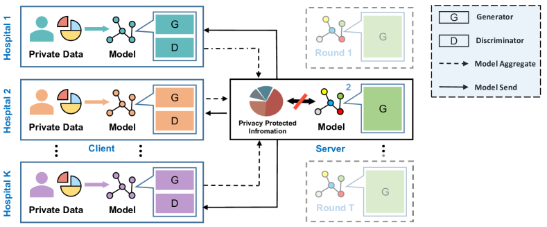
Figure 1: The pipeline of FedMed-GAN. The generator of each client participates in federated learning, while the discriminator of each client does not.

3 FedMed-GAN

Federated Model Setup. The federated setting of our generator and discriminator is described in Fig. 1. We employ CycleGAN (Zhu et al., 2017), MUNIT (Huang et al., 2018), UNIT (Liu et al., 2017), HLHGAN (Huang et al., 2020b), and Hyper-GAN (Yang et al., 2021) as our baseline models. Our baseline methods have two generators $G_{A\leftrightarrow B}$, discriminators $D_{A\leftrightarrow B}$. $G_{A\rightarrow B}$ generates B-modal images from A-modal samples. $D_{A\rightarrow B}$ distinguishes whether the generated B-modal data from A-modal samples is fake. Two generators ($G_{A\rightarrow B}$, $G_{B\rightarrow A}$) of each client joins in the aggregation process of FedAvg 1. In other words, the generators are separately aggregated into the server’s generators. Then, the server sends its generators into different hospitals. Moreover, according to GS-WGAN (Chen et al., 2020a), locating the discriminators ($D_{A\rightarrow B}$, $D_{B\rightarrow A}$) of each client locally can further increase the level of privacy preserving. Thus, the discriminators ($D_{A\rightarrow B}$, $D_{B\rightarrow A}$) are retained locally and do not participate in aggregation process.

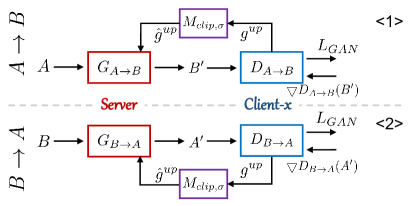
Figure 2: The architecture of FedMed-GAN, equipped with CycleGAN by adopting DP. The generator $G$ indicates that the models are shared with servers and clients. The discriminator $D$ indicates that the models are located in the client without sharing with one another. $M$ denotes the DP-SGD operator. $g^{up}$ denotes the back-propagation gradient from discriminators to generators. $\hat{g}^{up}$ denotes the clipped gradient after $M$.

Differential Privacy. Considering the superiority of DP-SGD (Abadi et al., 2016) and GS-WGAN (Chen et al., 2020b), we provide a differential privacy (DP) mechanism and show the detailed architecture in Fig. 2. The definition of differential privacy (Dwork and Roth, 2014) is defined as below:

Definition 1. A random mechanism $\mathcal{A}_{p}$ satisfies $(\epsilon,\delta)$-differential privacy if for any output’s subset ($\mathcal{S}$) and any two datasets $\mathcal{M}$, $\mathcal{M^{{}^{\prime}}}$, the following probability inequality holds:

$$\mathbb{P}(\mathcal{A}_{p}(\mathcal{M}\in\mathcal{S})\leq e^{\epsilon}\cdot\mathcal{P}(\mathcal{A}_{p}(\mathcal{M^{{}^{\prime}}}\in\mathcal{S})+\delta,$$ (1)

where $\delta>0$ and $\epsilon$ is the privacy budget indicating the privacy level, i.e., a smaller value of $\epsilon$ implies stronger privacy protection. To prevent privacy leakage from the server’s generators, we train the client’s generators ($G_{A\rightarrow B}$, $G_{B\rightarrow A}$) in a privacy-preserving manner. DP-SGD (Abadi et al., 2016) is adopted by using our DP. To realize DP, DP-SGD clips the gradient to bound sensitivity and add a calibrated random noise to induce stochasticity.

We directly apply DP-SGD to the parameters $\theta_{G}$ of the generators since the discriminator does not participate in the federated learning stage,

$$g_{G}^{t} =\nabla_{\theta_{G}}\mathcal{L_{G}}(\theta_{G}^{t},\theta_{D}^{t}),$$ (2)

$$\hat{g}_{G}^{t} =M_{clip,\sigma}=clip(g^{t},C)+\mathcal{N}(0,\sigma^{2}C^{2}I),$$

$$\theta_{G}^{t+1} =\theta_{G}^{t}-\eta_{G}\hat{g}_{G}^{t},$$

where $t$ is the epoch number in training. $C$ denotes the clip bound of the gradient. $\sigma$ represents the standard deviation of Gaussian noise. $g_{G}$ is the back-propagation gradient from the generator loss. $\hat{g}_{G}$ is the clipped gradient after $M_{clip,\sigma}$. The relationship between the noise variance and differential variance is given as follows:

$$\sigma=\frac{2q}{\epsilon}\sqrt{n_{d}\textrm{log}\frac{1}{\delta}},$$ (3)

where $q$ and $n_{d}$ denote the sample probability for each instance and the total batch number of the local dataset, respectively.

Loss Function For the synthesis process: $A\rightarrow B$ and its discriminator $D_{B}$, its generator loss function is defined as:

$$\mathcal{L}_{G}=\mathbb{E}_{a\sim p_{data}(a)}\left[\textrm{log}(1-D_{B}(G(a)))\right].$$ (4)

And the discriminator loss function is defined as:

$$\mathcal{L}_{D}=\mathbb{E}_{b\sim p_{data}(b)}\left[\textrm{log}D_{B}(b)\right].$$ (5)

For the synthesis process: $B\rightarrow A$, its generator loss function and discriminator loss are similar to Eq. (4) and Eq. (5). The cycle-consistency loss function from (Zhu et al., 2017) is defined as below:

$$\mathcal{L}_{cycle}(A,\hat{A},B,\hat{B})=\mathbb{E}_{a\sim p_{data}(a)}\left[\left\|G_{2}(G_{1}(a))-a\right\|\right]_{1}$$ (6)

$$+\mathbb{E}_{b\sim p_{data}(b)}\left[\left\|G_{1}(G_{2}(b))-b\right\|\right]_{1}.$$

4 Misaligned Unpaired Data (MUD)

We address the task of federated self-supervised learning for MUD by formulating several realistic settings. To simulate the real data distribution as much as possible, we adopt the following settings as shown in Fig. 3.

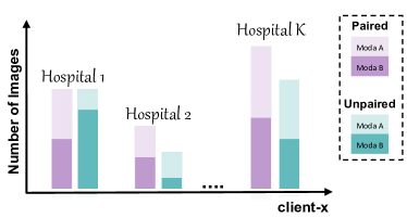
Figure 3: Examples of data distribution and performance during training.

Firstly, we divide ready-made data into several clients, where each client has its own private and unique data. Meanwhile, these clients (hospitals) contain unbalanced multi-modal images, i.e. having different numbers of patients in each client or having different numbers of images in each modality. Secondly, without losing generality, we explore both paired and unpaired cases in our experiments. For example, we randomly select the multi-modal slices from the same patient as paired data like in Hospital 1 or select them from patients with different IDs as unpaired data like in Hospital 2. After that, we randomly transform the input images at a certain threshold of rotation, translation and scaling, and there is the majority of misaligned images in the constructed training set.

5 Algorithm

The aggregation algorithm for the server’s generator is denoted in Algorithm 1, the client’s generator optimization algorithm is described in Algorithm 2, and the client’s discriminator algorithm is described in Algorithm 3.

Data: total number of hospitals $N\in\mathbb{N}$, total number of rounds of $T\in\mathbb{N}$, $G(A\rightarrow B)$: $G1$, $G(B\rightarrow A)$: $G2$, $D(A\rightarrow B)$: $D_{1}$, $D(B\rightarrow A)$: $D_{2}$: clients $\theta_{n}$, server $\theta_{S}$

Initialize: gen. $\theta^{0}_{G1}$ and $\theta^{0}_{G2}$, dis. $\theta^{0}_{D1}$ and $\theta^{0}_{D2}$

for each round $t$ from $0$ to $T$ do

       for each hospital $n\in N$ in parallel do

             $\theta^{t+1}_{n:G1},\theta^{t+1}_{n:G2}\leftarrow\mathrm{ClientGenUpdate}(\theta^{t}_{G1},\theta^{t}_{D1},\theta^{t}_{G2},\theta^{t}_{D2})$

             $\theta^{t+1}_{n:D1},\theta^{t+1}_{n:D2}\leftarrow\mathrm{ClientDiscUpdate}(\theta^{t}_{D1},\theta^{t}_{D2})$

            

       end for

      $\theta^{t+1}_{S:G1},\theta^{t+1}_{S:G1}\leftarrow\mathrm{Aggregate}(\theta^{t+1}_{n:G1},\theta^{t+1}_{n:G2})$

      

end for

Return: server generators $\theta_{G1}$, $\theta_{G2}$

Algorithm 1 Server-orchestrated training loop

Data: total number of steps $J\in\mathbb{N}$, batch size $S\in\mathbb{R}^{+}$, learning rate $\eta_{G}\in\mathbb{R}^{+}$, gen. input size $n_{U}\in\mathbb{N}$, $A_{fake}=A^{\prime}$, $B_{fake}=B^{\prime}$, $G(A\rightarrow B)$: $G_{1}$, $G(B\rightarrow A)$: $G_{2}$, $\hat{A}=G_{2}(B^{\prime})$, $\hat{B}=G_{1}(A^{\prime})$, clip bound $C$, noise standard deviation $\sigma$, gradient sensitization mechanism $\mathcal{M}$,

Loss function:$L_{G_{1}}(\theta_{G1},\theta_{D1};B^{\prime})$, $L_{G_{2}}(\theta_{G2},\theta_{D2};A^{\prime})$, $L_{cycle}(A,\hat{A},B,\hat{B})$

Initialize: $\theta_{G1}\leftarrow\theta^{0}_{G1}$, $\theta_{G2}\leftarrow\theta^{0}_{G2}$, $s\leftarrow$ $k$’s paired or unpaired data split into $S$ batches

for each generator training step $j$ from $1$ to $J$ do

       $U_{A}\leftarrow$ (sample $S$ random vectors of dim. $n_{U}$)

       $U_{B}\leftarrow$ (sample $S$ random vectors of dim. $n_{U}$)

       $A^{\prime}\leftarrow G(U_{B},\theta_{G})$

       $B^{\prime}\leftarrow G(U_{A},\theta_{G})$

       $g_{1}=\bigtriangledown(\mathcal{L}_{G1}(\theta_{G1},B^{\prime};\theta_{D1})+\mathcal{L}_{cycle})$

       $g_{2}=\bigtriangledown(\mathcal{L}_{G2}(\theta_{G2},A^{\prime};\theta_{D2})+\mathcal{L}_{cycle})$

       $\hat{g}_{1}=\mathcal{M}(g_{1})=\mathrm{clip}(g_{1},C)+N(\sigma^{2}C^{2}I)$

       $\hat{g}_{2}=\mathcal{M}(g_{2})=\mathrm{clip}(g_{2},C)+N(\sigma^{2}C^{2}I)$

       $\theta_{G1}=\theta_{G1}-\eta_{G}\hat{g}_{1}$

       $\theta_{G2}=\theta_{G2}-\eta_{G}\hat{g}_{2}$

      

end for

Return: client generators $\theta_{G1}$, $\theta_{G2}$

Algorithm 2 ClientGenUpdate($\theta_{D1}$, $\theta_{G1}$, $\theta_{D2}$, $\theta_{G2}$)

Data: number of steps $J\in\mathbb{N}$, batch size $S\in\mathbb{R}^{+}$, learning rate $\eta_{G}\in\mathbb{R}^{+}$, gen. input size $n_{U}\in\mathbb{N}$, $A_{fake}=A^{\prime}$, $B_{fake}=B^{\prime}$, $G(A\rightarrow B)$: $G_{1}$, $G(B\rightarrow A)$: $G_{2}$, $D(A\rightarrow B)$: $D_{1}$, $D(B\rightarrow A)$: $D_{2}$

Loss function: $L_{D_{1}}(\theta_{D1};B,B^{\prime})$, $L_{D_{2}}(\theta_{D2};A,A^{\prime})$

Initialize: $\theta_{D1}\leftarrow\theta^{0}_{D1}$, $\theta_{D2}\leftarrow\theta^{0}_{D2}$, $s\leftarrow$ $k$’s unpaired data split into $S$ batches

for each generator training step $j$ from $1$ to $J$ do

       $U_{A}\leftarrow$ (sample $S$ random vectors of dim. $n_{U}$)

       $U_{B}\leftarrow$ (sample $S$ random vectors of dim. $n_{U}$)

       $B^{\prime}\leftarrow G_{1}(U_{A},\theta_{G1})$

       $A^{\prime}\leftarrow G_{2}(U_{B},\theta_{G2})$

       $\theta_{D1}=\theta_{D1}-\eta_{D}\bigtriangledown(\mathcal{L}_{D1}(\theta_{D1};B,B^{\prime})$

       $\theta_{D2}=\theta_{D2}-\eta_{D}\bigtriangledown(\mathcal{L}_{D2}(\theta_{D2};A,A^{\prime})$

      

end for

Return: client generator $\theta_{D1}$ and $\theta_{D2}$

Algorithm 3 ClientDiscUpdate($\theta_{D1}$, $\theta_{D2}$)

6 Experiments

6.1 Implementations

IXI (Aljabar et al., 2011) collects nearly 600 MR images from normal and healthy subjects at three hospitals. The MR image acquisition protocol for each subject includes T1, T2, PD-weighted images (PD), MRA images, and Diffusion-weighted images (15 directions). Here, we only use T1 (581 cases), T2 (578 cases), and PD (578 cases) data to conduct our experiments, and select the paired data with the same ID from the three modes. The image has a non-uniform length on the z-axis with the size of $256$ on the x-axis and the y-axis. The IXI data set is not divided into a training set and a test set. Therefore, we randomly split the whole data as the training set (0.8) and the test set (0.2).

BraTS2021 (Siegel et al., 2019; Bakas et al., 2017) is constructed for analysis and diagnosis of brain disease. The publicly available dataset of multi-institutional pre-operative MRI sequences is provided: training (1251 cases) and validation (219 cases). Each patient contributes 155$\times$240$\times$240 with four sequences: T1, T2, T1ce, and FLAIR.

Metrics. We employ three metrics to evaluate our generator’s performance. The first is the mean absolute error (MAE):

$$\small MAE=\frac{1}{nm}\sum_{n}^{i=1}\sum_{m}^{j=1}\left|T_{ij}-G_{ij}\right|,$$ (7)

where $T_{ij}$ denotes the ground truth neuroimage pixel and $G_{ij}$ denotes the generated neuroimage pixel. The lower value of MAE means the better performance.

The second metric is the peak signal-to-noise ratio (PSNR). PSNR is a function of the mean squared error and is better to evaluate the context (edge) detail of neuroimages. The higher PSNR value means the better performance.

$$\small PSNR=-10\>log_{10}\left(\frac{1}{nm}\sum_{n}^{i=1}\sum_{m}^{j=1}(T_{ij}-G_{ij})^{2}\right).$$ (8)

The third metric is structural similarity index (SSIM), which is a weighted combination of the luminance, the contrast and the structure. A higher SSIM value means the better performance.

$$\small\mathrm{SSIM}=\frac{\left(2\mu_{T}\mu_{G}+C_{1}\right)\left(2\sigma_{TG}+C_{2}\right)}{\left(\mu_{T}^{2}+\mu_{G}^{2}+C_{1}\right)\left(\sigma_{T}^{2}+\sigma_{G}^{2}+C_{2}\right)}.$$ (9)

The $\mu$ and $\sigma$ in SSIM are the mean value and standard deviation of an image, respectively. $C_{1}$ and $C_{2}$ are two positive constants. We set $C_{1}$ and $C_{2}$ are 0.01 and 0.03, respectively.

Federated Data Setting. First, to ensure the validity and diversity of the data, we select 50 to 80 z-axis slices for each three-dimensional volume. The size of the data is uniformly cropped to 256 by 256 pixels. Second, to simulate data distributions in each client as closely as possible to real-world scenarios, we primarily divide the training data (volumes) proportionally among the predefined clients, where each client has its own private and unique ones. Using private data, we then construct paired and unpaired data based on the ratio specified for each client. Consequently, we can construct data patterns by adjusting the ratio between them (see Fig. 3).

Hyperparameter Setting. We use the learning rate of $1e-4$ and the batch size of 4. The optimizer is Adam (kingma2014adam). Its beta1 and beta2 are 0.5 and 0.999, respectively. The weights of GAN loss $\lambda_{adv}$ and Cycle loss $\lambda_{cyc}$ are 1.0, 10.0, respectively. In FedMed-GAN differential privacy settings, the levels of gradient clip bound, sensitivity, and noise multiplier are fixed to 1.0, 2.0, and 1.07, respectively. In terms of the differential privacy setting, the Gaussian noise $\mu$ is set to 1.07, and the standard deviation $\sigma$ is set to 2.0. The clip bound for the back-propagation gradient is set to 1.0.

6.2 Analysis of FedMed-GAN

From Table 1 and Table 2, we observe that FedMed-GAN does not sacrifice any performance under DP, and produces even better results compared with centralized training in almost all cases. In the experiment, we use 6000 images for both centralized and federated training. The ratio of paired data and unpaired data is fixed to 0.5. We set 30 epochs of centralized learning and 10 rounds of federated learning before aggregating the local models using FedAvg (McMahan et al., 2017a), in which each client is trained with 3 epochs in one round. In federated scenario, the weights of client data are set to 0.4, 0.3, 0.2, and 0.1, respectively.

Table 1: Baseline results on the BraTS2019 dataset.

	Method	Indicator	T1 $\rightarrow$ T2	T1 $\rightarrow$ FLAIR	T2 $\rightarrow$ T1	T2 $\rightarrow$ FLAIR	FLAIR $\rightarrow$ T1	FLAIR $\rightarrow$ T2
Non-Fed.	MUNIT	MAE $\downarrow$	0.0452	0.0492	0.0466	0.0459	0.0382	0.0420
		PSNR $\uparrow$	21.743	19.818	20.123	20.141	21.623	21.721
		SSIM $\uparrow$	0.8980	0.8853	0.9371	0.9023	0.9543	0.9117
	UNIT	MAE $\downarrow$	0.0437	0.0507	0.0536	0.0487	0.0482	0.0410
		PSNR $\uparrow$	20.833	20.190	20.067	20.266	20.493	21.212
		SSIM $\uparrow$	0.8855	0.8936	0.9313	0.8930	0.9338	0.9101
	CycleGAN	MAE $\downarrow$	0.0567	0.0535	0.0557	0.0462	0.0471	0.0454
		PSNR $\uparrow$	19.244	20.098	19.012	20.683	20.315	20.979
		SSIM $\uparrow$	0.8427	0.8984	0.9192	0.9140	0.9371	0.9003
	HLHGAN	MAE $\downarrow$	0.0217	0.0234	0.0245	0.0237	0.0246	0.0254
		PSNR $\uparrow$	30.847	30.578	30.876	30.847	30.702	30.689
		SSIM $\uparrow$	0.8127	0.8137	0.8145	0.8167	0.8130	0.8146
	Hyper-GAN	MAE $\downarrow$	0.0073	0.0071	0.0081	0.0083	0.0084	0.0082
		PSNR $\uparrow$	31.805	31.901	30.894	30.521	30.456	30.745
		SSIM $\uparrow$	0.9270	0.9310	0.9057	0.9032	0.9021	0.9128
Fed.	MUNIT	MAE $\downarrow$	0.0783	0.0934	0.0972	0.0960	0.1031	0.0782
		PSNR $\uparrow$	16.653	15.377	15.724	15.275	14.931	17.048
		SSIM $\uparrow$	0.6850	0.6463	0.8325	0.6402	0.8048	0.7114
	UNIT	MAE $\downarrow$	0.2631	0.2458	0.3461	0.2331	0.3443	0.3150
		PSNR $\uparrow$	9.3403	9.5427	7.9660	10.284	7.4321	7.6504
		SSIM $\uparrow$	0.0563	0.2066	0.0359	0.1768	0.0187	0.0555
	CycleGAN	MAE $\downarrow$	0.0609	0.0565	0.0565	0.0508	0.0470	0.0591
		PSNR $\uparrow$	18.506	18.620	18.620	19.904	20.540	19.402
		SSIM $\uparrow$	0.8507	0.9146	0.9146	0.8954	0.9405	0.8666
	HLHGAN	MAE $\downarrow$	0.0225	0.0242	0.0256	0.0257	0.0249	0.0261
		PSNR $\uparrow$	30.852	30.523	30.456	29.843	29.478	29.587
		SSIM $\uparrow$	0.8032	0.8131	0.8121	0.8135	0.8042	0.8212
	Hyper-GAN	MAE $\downarrow$	0.0082	0.0081	0.0092	0.0085	0.0094	0.0086
		PSNR $\uparrow$	31.905	31.575	29.894	30.323	30.578	30.812
		SSIM $\uparrow$	0.9183	0.9237	0.9057	0.9032	0.9046	0.9217

Table 2: Baseline results on the IXI dataset.

	Method	Indicator	T2 $\rightarrow$ PD	PD $\rightarrow$ T2
Non-Fed.	MUNIT	MAE $\downarrow$	0.0366	0.0324
		PSNR $\uparrow$	23.498	23.994
		SSIM $\uparrow$	0.9666	0.9524
	UNIT	MAE $\downarrow$	0.0417	0.0356
		PSNR $\uparrow$	22.671	23.000
		SSIM $\uparrow$	0.9575	0.9380
	CycleGAN	MAE $\downarrow$	0.0356	0.0315
		PSNR $\uparrow$	24.702	24.145
		SSIM $\uparrow$	0.9715	0.9516
	HLHGAN	MAE $\downarrow$	0.0372	0.0352
		PSNR $\uparrow$	30.045	30.176
		SSIM $\uparrow$	0.8872	0.8745
	Hyper-GAN	MAE $\downarrow$	0.0137	0.0148
		PSNR $\uparrow$	30.521	30.307
		SSIM $\uparrow$	0.9117	0.9139
Fed.	MUNIT	MAE $\downarrow$	0.1093	0.0842
		PSNR $\uparrow$	16.263	17.057
		SSIM $\uparrow$	0.8393	0.7033
	UNIT	MAE $\downarrow$	0.9800	0.2570
		PSNR $\uparrow$	9.4781	8.8979
		SSIM $\uparrow$	0.1587	0.0471
	CycleGAN	MAE $\downarrow$	0.0401	0.0364
		PSNR $\uparrow$	24.061	23.824
		SSIM $\uparrow$	0.9666	0.9472
	HLHGAN	MAE $\downarrow$	0.0275	0.0273
		PSNR $\uparrow$	30.031	29.852
		SSIM $\uparrow$	0.8653	0.8677
	Hyper-GAN	MAE $\downarrow$	0.0132	0.0133
		PSNR $\uparrow$	29.641	29.342
		SSIM $\uparrow$	0.9103	0.9098

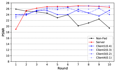
Figure 4: Results of FedMed-GAN training through multiple communication rounds.

Fig. 4 shows ablation studies of multiple communication rounds on the IXI dataset. Note that the red line indicates the performance of the server’s generator in FedMed-GAN. The blue line denotes the performance of generator under the centralized training. We observe that FedMed-GAN is able to stabilize the training dynamics of the generator, and gradually increase the performance of the server’s generator. However, the mode collapse problem occurs in the centralized training method. We also note that the performance of generator starts to deteriorate in the 21$th$ epoch from Fig. 4.

6.2.1 Multiple Clients and Data Distribution

We examine the effectiveness of FedMed-GAN when confronted with long-tail data phenomena. Table 3 demonstrates that FedMed-GAN is more stable. In Table 3, we divide the data distribution method into [‘average’, ‘gradual’, ‘extreme’]. For instance, when the client number is 4 and the proportion is 0.7+0.1$\times$3 (extreme mode). It indicates that the original data assign 70% to the first client and 10% to each of the remaining three clients.

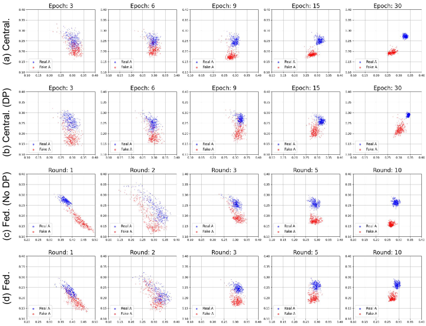
Figure 5: Visualization of sample’s features, which are generated by FedMed-GAN and centralized training.

Table 3: Results of FedMed-GAN on IXI (PD $\rightarrow$ T2).

Scheme	Client Num.	2	4	8
Average	Proportion	0.5 $\times$ 2	0.25 $\times$ 4	0.125 $\times$ 8
	MAE $\downarrow$	0.0258	0.0199	0.0219
	PSNR $\uparrow$	26.9717	28.0443	27.4549
	SSIM $\uparrow$	0.9736	0.9785	0.9775
Gradual	Proportion	0.6 + 0.4	0.4 + 0.3 + 0.2 + 0.1	0.3 + 0.2 + 0.1 $\times$ 4 + 0.05 $\times$ 2
	MAE $\downarrow$	0.0252	0.0203	0.0204
	PSNR $\uparrow$	27.4915	27.7578	27.8672
	SSIM $\uparrow$	0.9776	0.9787	0.9787
Extreme	Proportion	0.9 + 0.1	0.7 + 0.1 $\times$ 3	0.3 + 0.1 $\times$ 7
	MAE $\downarrow$	0.0264	0.0222	0.0218
	PSNR $\uparrow$	26.8523	27.5999	28.1727
	SSIM $\uparrow$	0.9737	0.9783	0.9889

6.2.2 Latent Space of Generators

To deeply investigate why FedMed-GAN can outperform the centralized training, we visualize the latent space of generators for FedMed-GAN and centralized training, respectively. In specific, the generator of CycleGAN is U-Net (Ronneberger et al., 2015). We take the down-sample layer 5 of U-Net as the latent space. After that, we divide the last dimension of the extracted vector into two dimensions (denoted as x and y), and reduce the vector by averaging the remaining dimensions. In Fig. 5, we plot 400 samples randomly selected in each modality.

The main differences between our FedMed-GAN and the centralized training are FedAvg (McMahan et al., 2017a) and DP-SGD (Abadi et al., 2016). We provide ablation studies for these two parts and evaluate whether they play an important role in stabilizing the training dynamics of GAN. The aim of cross-modality neuroimaging data is to pursue high fidelity and global diversity. The global diversity refers to the variety of neuroimaging data points as a whole. The cross-modality natural image synthesis attempts to synthesize each image into multiple styles as opposed to a single style. As for fidelity, we can obtain the results from the overlapped size of the latent space between the real ones. As the overlapped size becomes larger, the fidelity of the generated samples becomes higher. For global diversity, we can obtain the results from the variance of latent space of the generated samples, i.e. fake A and fake B. Therefore, as the variance becomes higher, the global diversity gets much higher.

6.2.3 Notation

In Fig. 5, modal A is PD-weighted MRI data and modal B is T2-weighted MRI data from IXI. The red dots denote the distributions of the latent space for modal A. The blue dots are the distributions of the latent space for the generated samples of modal A (termed as fake A). The green dots are the distributions of the latent space for modal B. The black dots are the distributions of the latent space for the generated samples of modal B (termed as fake B). Fig. 5(a) denotes the centralized training method for CycleGAN. Fig. 5(b) denotes the centralized training method combined with DP-SGD. Fig. 5(c) denotes the FedAvg algorithm without DP-SGD. Fig. 5(d) denotes the FedAvg algorithm combined with DP-SGD.

6.2.4 Differential Privacy

(1) FedAvg+DPSGD vs FedAvg? Firstly, we investigate the role of DP. When comparing Fig. 5(c) and Fig. 5(d), we observe that FedAvg+DPSGD outperforms FedAvg. Also, the diversity of fake A in FedAvg+DP-SGD is significantly greater than in FedAvg without DPSGD. In addition, from round 5 to round 10, the distance between the real A and the fake A in FedAvg+DPSGD decreases, whereas the latent space between the real A and the fake A in FedAvg without DP-SGD gradually increases. It suggests that DP-SGD stabilizes the training dynamics of GAN.

Table 4: Noise comparisons on the IXI dataset.

Noise	Clip-Bound	0.7	1.0	1.3
0.5	MAE  $\downarrow$	0.0198	0.0200	0.0226
	PSNR $\uparrow$	27.8496	27.934	27.8617
	SSIM $\uparrow$	0.9787	0.9794	0.9786
1.07	MAE  $\downarrow$	0.0212	0.0203	0.0201
	PSNR $\uparrow$	28.0310	27.7578	27.7840
	SSIM $\uparrow$	0.9801	0.9787	0.9786
2.0	MAE  $\downarrow$	0.0203	0.0204	0.0222
	PSNR $\uparrow$	27.8385	27.8125	27.8149
	SSIM $\uparrow$	0.9784	0.9786	0.9782

Table 5: Centralized training with more discriminators on the IXI dataset. D denotes the number of the discriminators. Each grid’s value is the PSNR score.

Epoch	D=2	D=4	D=8
1	25.1043	24.8932	24.9375
6	24.1453	23.9843	23.7685
9	23.6572	23.3483	22.5643
15	21.4587	21.3987	20.8761
18	20.8875	20.8846	20.1698
24	19.2497	19.1430	18.9456
30	18.2768	18.3674	18.3654

Table 6: Centralized training with more discriminators on the BraTS dataset. D denotes the number of discriminators. Each grid’s value is the PSNR score.

Epoch	D=2	D=4	D=8
1	18.9329	18.2671	18.1451
6	19.3435	18.9982	18.9213
9	18.3467	18.1656	18.1345
15	17.6589	17.4532	17.2869
18	16.6945	16.5672	16.4783
24	16.2497	15.9843	15.7566
30	15.9345	15.6756	15.6783

(2) Central+DPSGD vs Central? Furthermore, we add DP-SGD into the centralized training, as described in Fig. 5(b). Although adding DP-SGD into the centralized training is unnecessary, we desire to verify our assumption that DP-SGD can be treated as a gradient penalty to prevent mode collapse. Compared with Fig. 5(a) and Fig. 5(b), we can find that the global diversity of fake A is much larger in centralized training+ DP-SGD than the ones in centralized training in the absence of DP-SGD after epoch 12. The distance between fake A and real A becomes larger in centralized training without DP-SGD after epoch 9. However, the distribution of fake A and real A is much farther after epoch 9. We think that DP-SGD can be one of the important measures to facilitate the convergence of GAN. Rethinking the Eq. (1) to Eq. (3), we find that DP-SGD works as a gradient penalty, which has been proved as one of simple but effective approach to regularize the training dynamics of GAN (Mescheder et al., 2018). Such a result has concurred with each other in this view. Finally, to evaluate the hyperparameters of clip bound and noise density in DP, we perform relevant experiments and find that the performance of FedMed-GAN is very stable with various DP guarantees. These results are provided in Table 4.

6.2.5 FedAvg

Despite DP-SGD, FedAvg in Algorithm 1 also plays an important role in stabilizing the training. Compared with Fig. 5(a) and Fig. 5(d), the distance between real A samples and fake A samples is gradually smaller in FedAvg after epoch 9. However, the distributions of real A and fake A are gradually distant in the centralized training after epoch 9. The Fed-Avg method aggregates the weight from each client’s generator and edge network to the server model according to the data proportion distribution. The manifolds of the generators (the server’s generators and the clients’ ones) in FedMed-GAN are reparamterized, which are consistent with the assumption of convergence proof in Mescheder et al. (Mescheder et al., 2018).

Table 7: Centralized Training + DP-SGD. ’w’ denotes the centralized training with DP-SGD. ’w/o’ denotes the centralized training without DP-SGD. Each grid’s value is the PSNR score.

Dataset	Epoch	1	4	7	10	13	16	19	21	24	27	30
IXI	w/o	23.69	25.03	24.10	25.30	24.91	23.11	23.49	20.18	21.16	22.50	19.42
(PD-T2)	w	25.67	25.67	25.98	24.23	23.41	20.68	21.07	23.69	18.91	20.71	21.79
BraTS	w/o	18.20	18.28	18.67	19.40	18.78	18.47	17.39	17.74	19.47	17.51	18.47
(T1-FLAIR)	w	19.34	19.94	19.20	19.43	19.53	19.50	19.53	19.40	18.95	19.61	16.82

6.2.6 Centralized+More Discriminators

We add more discriminators in the centralized training experiment and the results are listed in Table 5 and Table 6. The number of discriminators is the same as the number of clients in federated learning. We average the logits from multiple discriminators for the training and testing. The results are provided here, which show that adding more discriminators is not able to stabilize the training dynamics. We think that the largest difference between centralized training and FedMed-GAN is a FedAvg algorithm. In addition, in the original paper, we have illustrated that the role of FedAvg is to (Mescheder et al., 2018).

6.2.7 Centralized+DPSGD vs DPSGD

We conduct centralized training + DP-SGD on IXI (PD$\rightarrow$T2) dataset and BraTS (T1$\rightarrow$FLAIR) dataset. The results are listed in Table 7. We observe that centralized training + DP-SGD is not able to prevent mode collapse issue. We think that DP-SGD equals to gradient clipping and adding Gaussian noise to the clipped gradient. The discriminator overfitting problem is the main reason for mode collapse issue. The discriminator over-fitting can result in the gradient vanishing problem (i.e., the gradient is very small). In this case, the gradient clipping mechanism is meaningless since the gradient norm is much smaller than the clip bound. We observe that the gradient norms in centralized training approximately reach to 0 when mode collapse happens. Thus, DP-SGD + Centralized Training cannot mitigate mode collapse issue. Instead, we observe that the gradient norms in centralized training approximately reach to 0 when mode collapse happen issue. The reason is that the data assigned for each client’s discriminator is limited. It is not easy to result in discriminator’s over-fitting and not easy to be stuck into the local optimum. Therefore, DP-SGD can help mitigate the mode collapse issue in FedMed-GAN.

Table 8: PSNR’s performance on various differential privacy budgets. In each grid, the first term is the privacy budget and the PSNR score performance $p$. $\delta$ denotes the standard deviation of Gaussian noise. $\epsilon$ is the privacy budget indicating the privacy level. The smaller $\epsilon$ value implies stronger privacy protection.

($\epsilon$, $\delta$)	2 clients	4 clients	8 clients
noise=0.5	(813.79, 1e-5), $p$: 27.4678	(505.26, 1e-5), $p$: 28.0123	(250.44, 1e-5), $p$=27.1564
noise=1.07	(200.47, 1e-5) $p$: 27.7341	(74.36, 1e-05), $p$: 28.1374	(28.83, 1e-5), $p$=27.1432
noise=2.0	(71.51, 1e-5) $p$: 27.8921	(27.98, 1e-5), $p$: 28.1475	(12.92, 1e-5), $p$=27.1876

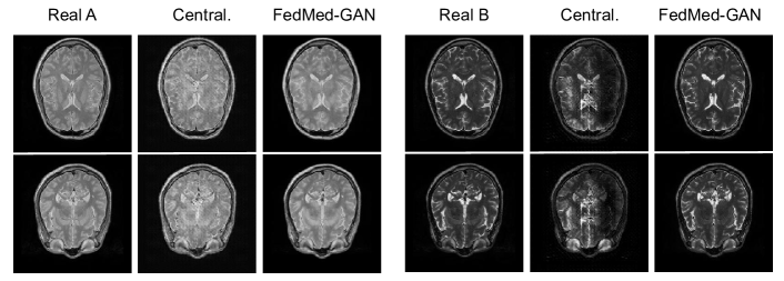
Figure 6: Visualization of FedMed-GAN. We use the results of 24$th$ epoch of centralized training (Central.) and 8$th$ round of FedMed-GAN as examples (IXI, PD $\leftrightarrow$ T2).

6.2.8 Privacy Budget

According to Eq. (3), we calculate the privacy budget with various Gaussian noises. From Table 8, we find that the synthesis quality of FedMed-GAN is not affected by the different privacy budgets. It also indicates the robustness of FedMed-GAN.

6.2.9 Noise Comparisons in DP

Moreover, we desire to know whether the effect resulted from DP-SGD are very sensitive to the hyper-parameter setting or not. So if yes, it may violate our explanations mentioned above. But from Table 4, we find that the performance of FedMed-GAN is very stable with various DP guarantees.

7 Visualization

Fig. 6 presents visualization resulting achieved by FedMed-GAN. Real A (PD) and Real B (T2) are the ground-truth neuroimage. Cetralized denotes the synthesis neuroimage via centralized training. FedMed-GAN denotes the synthesis neuroimage by FedMed-GAN. From Fig. 6, we can observe that FedMed-GAN can generate high-quality images with vivid information of brain tissues, compared with ones generated by centralized training.

8 Conclusion

In this paper, we propose a novel baseline FedMed-GAN for unsupervised cross-modality brain image synthesis in federated manner. We find that both DP and the federated averaging mechanism can effectively improve the ability of the model generation, showing advantages over the centralized training. Experimental results show that FedMed-GAN can generate clear images, providing a powerful model for the field of federated domain translation. Limitations and Future Work: The performance of FedMed-GAN has not been verified by the radiologist and the interpretability needs to be explored in the future.

Declaration of Competing Interest

The authors declare that they have no known competing financial interests or personal relationships that could have appeared to influence the work reported in this paper.

authors/jinbao-wang1 Jinbao Wang received the Ph.D. degree from the University of Chinese Academy of Sciences (UCAS) in 2019. He is currently a Research Assistant Professor with the Southern University of Science and Technology (SUSTech), Shenzhen, China. His research interests include machine learning, computer vision, image anomaly detection, and graph representation learning.

authors/xie1 Guoyang Xie received the Bachelor and MPhil Degrees from University of Electronic Science and Technology of China, Hong Kong University of Science and Technology in 2009 and 2013, respectively. He is pursuing the PhD degree from University of Surrey. Prior to that, he was the Principle Perception Algorithm Engineer in Baidu and GAC, respectively. His research interests include anomaly detection, medical imaging, neural architecture search and federated learning.

authors/huang Yawen Huang received the M.Sc. and Ph.D. degrees from the Department of Electronic and Electrical Engineering, The University of Sheffield, Sheffield, U.K., in 2015 and 2018, respectively. She is currently a Senior Scientist of Tencent Jarvis Laboratory, Shenzhen, China. Her research interests include computer vision, machine learning, medical imaging, deep learning, and practical AI for computer aided diagnosis.

authors/jiayi-lyu1 Lyu Jiayi, born in 1999, graduated in 2021 from Capital Normal University with a bachelor’s degree in computer science and technology. She is now pursuing a Ph.D. in computer applications at the School of Engineering Science, Chinese Academy of Sciences.

authors/feng-zheng Feng Zheng (Member, IEEE) received the Ph.D. degree from The University of Sheffield, Sheffield, U.K., in 2017. He is currently an Assistant Professor with the Department of Computer Science and Engineering, Southern University of Science and Technology, Shenzhen, China. His research interests include machine learning, computer vision, and human-computer interaction. authors/yefeng-zheng Yefeng Zheng (Fellow, IEEE) received the B.E. and M.E. degrees from Tsinghua University, Beijing, in 1998 and 2001, respectively, and the Ph.D. degree from the University of Maryland, College Park, MD, USA, in 2005. After graduation, he joined Siemens Corporate Research, Princeton, NJ, USA. He is currently the Director and the Distinguished Scientist of Tencent Jarvis Laboratory, Shenzhen, China, leading the company’s initiative on Medical AI. His research interests include medical image analysis, graph data mining, and deep learning. Dr. Zheng is a fellow of the American Institute for Medical and Biological Engineering (AIMBE). authors/yaochu-jin Yaochu Jin received the B.Sc., M.Sc., and Ph.D. degrees from Zhejiang University, Hangzhou, China, in 1988, 1991, and 1996, respectively, and the Dr.-Ing. degree from Ruhr University Bochum, Germany, in 2001.

He is presently an Alexander von Humboldt Professor for Artificial Intelligence endowed by the German Federal Ministry of Education and Research, Chair of Nature Inspired Computing and Engineering, Faculty of Technology, Bielefeld University, Germany. He is also a Distinguished Chair, Professor in Computational Intelligence, Department of Computer Science, University of Surrey, Guildford, U.K. He was a “Finland Distinguished Professor” of University of Jyväskylä awarded by the Academy of Science and Finnish Funding Agency for Innovation, Finland, and “Changjiang Distinguished Visiting Professor” of Northeastern University, awarded by the Ministry of Education, China. His main research interests include human-centered learning and optimization, synergies between evolution and learning, and evolutionary developmental artificial intelligence.

Prof. Jin is the President-Elect of the IEEE Computational Intelligence Society and the Editor-in-Chief of Complex & Intelligent Systems. He was named by Clarivate as a “Highly Cited Researcher” from 2019 to 2022 consecutively. He is a Member of Academia Europaea and Fellow of IEEE.

References

- Abadi et al. (2016) Abadi, M., Chu, A., Goodfellow, I., McMahan, H.B., Mironov, I., Talwar, K., Zhang, L., 2016. Deep learning with differential privacy, in: Proceedings of the 2016 ACM SIGSAC conference on computer and communications security, pp. 308–318.
- Aljabar et al. (2011) Aljabar, P., Wolz, R., Srinivasan, L., Counsell, S.J., Rutherford, M.A., Edwards, A.D., Hajnal, J.V., Rueckert, D., 2011. A combined manifold learning analysis of shape and appearance to characterize neonatal brain development. IEEE Transactions on Medical Imaging 30, 2072–2086.
- Augenstein et al. (2020) Augenstein, S., McMahan, H.B., Ramage, D., Ramaswamy, S., Kairouz, P., Chen, M., Mathews, R., y Arcas, B.A., 2020. Generative models for effective ML on private, decentralized datasets, in: ICLR, OpenReview.net.
- Bakas et al. (2017) Bakas, S., Kuijf, H.J., Menze, B.H., Reyes, M., 2017. Brainlesion: Glioma, multiple sclerosis, stroke and traumatic brain injuries, in: Lecture Notes in Computer Science.
- Chen et al. (2020a) Chen, D., Orekondy, T., Fritz, M., 2020a. Gs-wgan: A gradient-sanitized approach for learning differentially private generators. Advances in Neural Information Processing Systems 33, 12673–12684.
- Chen et al. (2020b) Chen, D., Orekondy, T., Fritz, M., 2020b. GS-WGAN: A gradient-sanitized approach for learning differentially private generators, in: NeurIPS.
- Dar et al. (2019) Dar, S.U.H., Yurt, M., Karacan, L., Erdem, A., Erdem, E., Çukur, T., 2019. Image synthesis in multi-contrast mri with conditional generative adversarial networks. IEEE Transactions on Medical Imaging 38, 2375–2388.
- Dwork and Roth (2014) Dwork, C., Roth, A., 2014. The algorithmic foundations of differential privacy. Found. Trends Theor. Comput. Sci. 9, 211–407.
- Goodfellow et al. (2014) Goodfellow, I., Pouget-Abadie, J., Mirza, M., Xu, B., Warde-Farley, D., Ozair, S., Courville, A., Bengio, Y., 2014. Generative adversarial nets. Advances in neural information processing systems 27.
- Guo et al. (2021) Guo, P., Wang, P., Yasarla, R., Zhou, J., Patel, V.M., Jiang, S., 2021. Anatomic and molecular mr image synthesis using confidence guided cnns. IEEE Transactions on Medical Imaging 40, 2832–2844.
- Huang et al. (2018) Huang, X., Liu, M.Y., Belongie, S., Kautz, J., 2018. Multimodal unsupervised image-to-image translation, in: Proceedings of the European conference on computer vision (ECCV), pp. 172–189.
- Huang et al. (2020a) Huang, Y., Zheng, F., Cong, R., Huang, W., Scott, M.R., Shao, L., 2020a. Mcmt-gan: Multi-task coherent modality transferable gan for 3d brain image synthesis. IEEE Transactions on Image Processing 29, 8187–8198.
- Huang et al. (2020b) Huang, Y., Zheng, F., Wang, D., Jiang, J., Wang, X., Shao, L., 2020b. Super-resolution and inpainting with degraded and upgraded generative adversarial networks, in: IJCAI.
- Jiang et al. (2019) Jiang, G., Lu, Y., Wei, J., Xu, Y., 2019. Synthesize mammogram from digital breast tomosynthesis with gradient guided cgans, in: International Conference on Medical Image Computing and Computer-Assisted Intervention, Springer. pp. 801–809.
- Kong et al. (2021) Kong, L., Lian, C., Huang, D., Hu, Y., Zhou, Q., et al., 2021. Breaking the dilemma of medical image-to-image translation. Advances in Neural Information Processing Systems 34, 1964–1978.
- Li et al. (2022) Li, H., Wu, P., Wang, Z., Mao, J.F., Alsaadi, F.E., Zeng, N., 2022. A generalized framework of feature learning enhanced convolutional neural network for pathology-image-oriented cancer diagnosis. Computers in biology and medicine 151 Pt A, 106265.
- Li et al. (2020) Li, T., Sahu, A.K., Zaheer, M., Sanjabi, M., Talwalkar, A., Smith, V., 2020. Federated optimization in heterogeneous networks, in: MLSys, mlsys.org.
- Liu et al. (2017) Liu, M., Breuel, T.M., Kautz, J., 2017. Unsupervised image-to-image translation networks, in: NIPS, pp. 700–708.
- Long et al. (2019) Long, Y., Wang, B., Yang, Z., Kailkhura, B., Zhang, A., Gunter, C., Li, B., 2019. G-pate: Scalable differentially private data generator via private aggregation of teacher discriminators, in: Neural Information Processing Systems.
- McMahan et al. (2017a) McMahan, B., Moore, E., Ramage, D., Hampson, S., y Arcas, B.A., 2017a. Communication-efficient learning of deep networks from decentralized data, in: Artificial intelligence and statistics, PMLR. pp. 1273–1282.
- McMahan et al. (2017b) McMahan, B., Moore, E., Ramage, D., Hampson, S., y Arcas, B.A., 2017b. Communication-efficient learning of deep networks from decentralized data, in: AISTATS, PMLR. pp. 1273–1282.
- Mescheder et al. (2018) Mescheder, L.M., Geiger, A., Nowozin, S., 2018. Which training methods for gans do actually converge?, in: ICML.
- Ren et al. (2021) Ren, M., Dey, N., Fishbaugh, J., Gerig, G., 2021. Segmentation-renormalized deep feature modulation for unpaired image harmonization. IEEE Transactions on Medical Imaging 40, 1519–1530.
- Ronneberger et al. (2015) Ronneberger, O., Fischer, P., Brox, T., 2015. U-net: Convolutional networks for biomedical image segmentation, in: MICCAI.
- Sharma and Hamarneh (2020) Sharma, A., Hamarneh, G., 2020. Missing mri pulse sequence synthesis using multi-modal generative adversarial network. IEEE Transactions on Medical Imaging 39, 1170–1183.
- Shen et al. (2021) Shen, L., Zhu, W., Wang, X., Xing, L., Pauly, J.M., Turkbey, B., Harmon, S.A., Sanford, T., Mehralivand, S., Choyke, P.L., Wood, B.J., Xu, D., 2021. Multi-domain image completion for random missing input data. IEEE Transactions on Medical Imaging 40, 1113–1122.
- Siegel et al. (2019) Siegel, R.L., Miller, K.D., Jemal, A., 2019. Cancer statistics, 2019. CA: A Cancer Journal for Clinicians 69.
- Song and Ye (2021) Song, J., Ye, J.C., 2021. Federated cyclegan for privacy-preserving image-to-image translation. CoRR abs/2106.09246.
- Wang et al. (2020) Wang, H., Yurochkin, M., Sun, Y., Papailiopoulos, D.S., Khazaeni, Y., 2020. Federated learning with matched averaging, in: ICLR, OpenReview.net.
- Wang et al. (2018) Wang, Y., Zhou, L., Wang, L., Yu, B., Zu, C., Lalush, D.S., Lin, W., Wu, X., Zhou, J., Shen, D., 2018. Locality adaptive multi-modality gans for high-quality pet image synthesis. Medical image computing and computer-assisted intervention : MICCAI … International Conference on Medical Image Computing and Computer-Assisted Intervention 11070, 329–337.
- Wu et al. (2023) Wu, P., Wang, Z., Zheng, B., Li, H., Alsaadi, F.E., Zeng, N., 2023. Aggn: Attention-based glioma grading network with multi-scale feature extraction and multi-modal information fusion. Computers in biology and medicine 152, 106457.
- Yang et al. (2021) Yang, H., Sun, J., Yang, L., Xu, Z., 2021. A unified hyper-gan model for unpaired multi-contrast mr image translation, in: International Conference on Medical Image Computing and Computer-Assisted Intervention.
- Yu et al. (2018) Yu, B., Zhou, L., Wang, L., Fripp, J., Bourgeat, P.T., 2018. 3d cgan based cross-modality mr image synthesis for brain tumor segmentation. 2018 IEEE 15th International Symposium on Biomedical Imaging (ISBI 2018) , 626–630.
- Yu et al. (2020) Yu, B., Zhou, L., Wang, L., Shi, Y., Fripp, J., Bourgeat, P.T., 2020. Sample-adaptive gans: Linking global and local mappings for cross-modality mr image synthesis. IEEE Transactions on Medical Imaging 39, 2339–2350.
- Yurochkin et al. (2019) Yurochkin, M., Agarwal, M., Ghosh, S., Greenewald, K.H., Hoang, T.N., Khazaeni, Y., 2019. Bayesian nonparametric federated learning of neural networks, in: ICML, PMLR. pp. 7252–7261.
- Zhou et al. (2021) Zhou, B., Liu, C., Duncan, J.S., 2021. Anatomy-constrained contrastive learning for synthetic segmentation without ground-truth, in: MICCAI.
- Zhu et al. (2017) Zhu, J.Y., Park, T., Isola, P., Efros, A.A., 2017. Unpaired image-to-image translation using cycle-consistent adversarial networks, in: Proceedings of the IEEE international conference on computer vision, pp. 2223–2232.
- Zuo et al. (2021) Zuo, Q., Zhang, J., Yang, Y., 2021. Dmc-fusion: Deep multi-cascade fusion with classifier-based feature synthesis for medical multi-modal images. IEEE Journal of Biomedical and Health Informatics 25, 3438–3449.