Exact wavefunction dualities and phase diagrams of 3D quantum vertex models

Abstract

We construct a broad class of frustration-free quantum vertex models in 3+1D whose ground states are weighted superpositions of classical 3D vertex model configurations. For the simplest members of this class, the corresponding classical vertex models have a $\mathbb{Z}_{2}$ gauge constraint enriched with a $\mathbb{Z}_{2}$ global symmetry. We deduce a phase diagram for the quantum vertex models using exact dualities and mappings to classical spin models and height models. We find $\mathbb{Z}_{2}$ deconfined and $\mathbb{Z}_{2}$ symmetry-broken phases which are mapped to one another by duality. The transition between these phases is governed by a self-dual gapless point which is related by a different duality to the Rokhsar-Kivelson (RK) point of quantum spin ice. Our results are illustrated for diamond and cubic lattices, but hold for general 3D lattices with even coordination number.

Introduction— Quantum spin liquids represent zero temperature phases of matter whose essential characteristics lie beyond the Landau order parameter paradigm [1]. Quantum dimer models represent a family of simplified models [2, 3, 4, 5, 6] in which novel properties of quantum spin liquids such as fractionalized excitations with anyonic statistics, emergent gauge bosons and ground state degeneracy can be readily accessed. Analytic progress is aided by the fact that at specially tuned Rokhsar-Kivelson (RK) points [3], correlation functions in the ground state of quantum dimer models are equivalent to corresponding correlators in classical dimer models [3, 7, 8, 9, 10]. Furthermore, on planar graphs, correlation functions of classical dimers can be exactly studied using the methods of Kasteleyn [11] and Temperley and Fisher [12]. However, such methods generally fail in 3+1D, where potentially exotic phases such as $U(1)$ spin liquids may emerge [13, 14, 15]. These methods also fail in the presence of multi dimer configurations, a common occurrence in frustrated systems such as those that obey the “ice-rule” constraint. Expanding the list of exactly solvable models in 3+1D will contribute significantly to our fundamental understanding of quantum spin models in 3D.

In this paper, we study a family of quantum spin models in 3+1D whose ground states are related to the partition function of 3D classical vertex models. Recall, a vertex model is defined in terms of closed loop configurations whose statistical weight is a product of vertex weights, which depend on the configuration at each individual vertex. Given a classical 3D vertex model with adjustable vertex weights, we construct analytically tractable 3+1D quantum spin models with multi-dimer constraints whose ground states are equivalent (in the RK sense) to the classical model for any allowed values of the vertex weights. We call these quantum vertex models [16]. We study the classical vertex model using Wegner’s weak graph duality [17, 18, 19, 20] and mappings to equivalent classical spin models and height models. Using these mappings, we exactly construct a phase diagram for the quantum vertex models as a function of the vertex weights. In particular, we find an unusual gapless point where both local order and deconfinement (defined in an appropriate sense) coexist. We then use an effective field theory to analyze deformations of the quantum model away from the RK point.

Quantum vertex models— We construct a Hamiltonian defined on a regular bipartite lattice in 3D with even coordination number. We will focus on two cases, where the bipartite lattice is (i) a diamond lattice, dual to the pyrochlore lattice of corner sharing tetrahedra and (ii) a cubic lattice, dual to a lattice of corner sharing octahedra. However, our approach is not limited to these two lattices, and our results generically hold for any even-coordinated lattice in 3D.

We start by briefly defining a classical vertex model, whose degrees of freedom are dimers on the links of the lattice. The classical Boltzmann weight $\mathcal{W}(C)$ of a configuration $C$ of dimers is the product of vertex weights $W_{V_{p}}(n_{C})$ at each site $p$, where $n_{C}$ is the number of dimers touching $p$ in configuration $C$ and $V_{p}$ is the coordination number: $\mathcal{W}(C)=\prod_{p}W_{V_{p}}(n_{C})$. The partition function is then $\mathcal{Z}=\sum_{C}\mathcal{W}(C)$. Motivated by this construction, we define an unnormalized RK ground state wavefunction $\ket{\text{GS}}=\sum_{C}\sqrt{\mathcal{W}(C)}\ket{C}$, whose norm is the partition function of the classical vertex model.

We now discuss the choice of vertex weights. Assume that configurations corresponding to $0$ or $V_{p}$ dimers touching a site have vertex weight $u$ and all other configurations with even $n$ have vertex weight $1$, while configurations with odd $n$ have vertex weight $0$. We note that these weights are invariant under the $\mathbb{Z}_{2}$ symmetry of exchanging dimers and empty links. Explicitly, for the 8-vertex model on a diamond lattice

$$W_{4}(0)=W_{4}(4)=u,\hskip 14.22636ptW_{4}(2)=1,$$ (1)

and for the 32-vertex model on a cubic lattice

$$W_{6}(0)=W_{6}(6)=u,\hskip 14.22636ptW_{6}(2)=W_{6}(4)=1.$$ (2)

We will prove the existence of a gapless point in the phase diagrams of both the diamond and cubic lattice models that corresponds to $u=3$ and $u=5$ respectively. In addition, we show that this gapless point is dual to an RK wavefunction satisfying an ice rule constraint on the respective lattice. On both diamond and cubic lattices, the ice rule constraint corresponds to known $U(1)$ spin liquid phases [14, 15]. Furthermore, the gapless boundary is present and can be exactly determined on any 3D lattice with even coordination number. Note that on the diamond lattice the point $u=0$ directly corresponds to the RK wavefunction of the pyrochlore spin ice model studied by Hermele, Fisher and Balents [14]; this is a property of any lattice with coordination number $V_{p}\in 4\mathbb{Z}$.

Next, we construct a parent Hamiltonian which annihilates the RK wavefunction $\ket{\text{GS}}=\sum_{C}\sqrt{\mathcal{W}(C)}\ket{C}$, and therefore shares the same RK phase diagram as the classical vertex model. Place spins on the edges of the diamond/cubic lattices (alternatively on the sites of the pyrochlore/octahedral lattices) with the interpretation that spin up corresponds to the presence of a dimer and spin down the absence of a dimer, and construct the unperturbed Hamiltonian(s):

$$\mathcal{H}_{0,\text{d}}=-J_{z}\sum_{\raisebox{-1.0pt}{\includegraphics[height=6.02777pt]{tetrahedron.png}}}\prod_{i\in\raisebox{-1.0pt}{\includegraphics[height=6.02777pt]{tetrahedron.png}}}Z_{i}\hskip 14.22636pt\mathcal{H}_{0,\text{c}}=-J_{z}\sum_{\raisebox{-4.0pt}{\includegraphics[height=9.04166pt]{octahedron.png}}}\prod_{i\in\raisebox{-4.0pt}{\includegraphics[height=9.04166pt]{octahedron.png}}}Z_{i},$$ (3)

The ground states of these Hamiltonians are classical configurations with an even number of dimers touching each site of the diamond/cubic lattice. Next, we add a perturbing interaction, which is an antiferromagnetic XY exchange between nearest neighbor spins in the pyrochlore and octahedral lattices:

$$\mathcal{H}=\mathcal{H}_{0}+J_{\perp}\sum_{\langle i,j\rangle}(X_{i}X_{j}+Y_{i}Y_{j}),$$ (4)

Performing standard degenerate perturbation theory, we find that

$$\mathcal{H}_{\text{eff}}\propto-\sum_{r}\left(\prod_{P\in r}\frac{1+\prod_{i\in P}Z_{i}}{2}\right)\prod_{j\in r}X_{j},$$ (5)

where $r$ indicates a plaquette where ring exchanges occur ($r=\mathord{\raisebox{-1.0pt}{ \leavevmode\hbox to7.48pt{\vbox to6.53pt{\text{[drawing]}}}}}$ for the diamond lattice and $r=\square$ for the cubic lattice), while $P$ indicates polyhedra ($P=\raisebox{-1.0pt}{\includegraphics[height=8.61108pt]{tetrahedron.png}}$ for the diamond lattice and $P=\raisebox{-4.0pt}{\includegraphics[height=12.91663pt]{octahedron.png}}$ for the cubic lattice). The notation $P\in r$ denotes the polyhedra which take part in the ring exchange around plaquette $r$. The proportionality constant scales like $O(J_{\perp}^{2}/J_{z})$ on the cubic lattice and $O(J_{\perp}^{3}/J_{z}^{2})$ on the diamond lattice. For convenience, we write $Z_{P}=\prod_{i\in P}Z_{i}$. Finally, we deform the Hamiltonian by adding a multi-spin interaction term $\mathcal{P}_{r}(u)$ of a fine-tuned nature

$$\mathcal{H}_{\text{eff}}\propto\sum_{r}\left(\prod_{P\in r}\frac{1+Z_{P}}{2}\right)\left(-\prod_{j\in r}X_{j}+(1-J)\mathcal{P}_{r}(u)\right),$$ (6)

such that the Hamiltonian becomes frustration-free at $J=0$ and the ground state is the desired RK wavefunction. We refer the reader to Supplementary material for an explicit construction of $\mathcal{P}_{r}(u)$. Schematically, this follows because $-\prod_{j\in r}X_{j}+\mathcal{P}_{r}(u)$ projects onto superpositions of vertex model configurations whose relative weights are consistent with the classical vertex weights. As in the classical vertex model, the quantum vertex model has a global $\mathbb{Z}_{2}$ spin-flip symmetry $\prod_{i}X_{i}$ interchanging dimers and empty links. For most of the remainder of the paper we work at $J=0$.

Dualities and phase diagrams— In 3D, classical vertex models are non-integrable with rare exceptions [21]; however, conveniently, vertex models possess an exact self-duality which is a special case of Wegner’s duality [17, 19, 18, 20]. This duality exactly relates the partition functions of classical vertex models at $u$ and $u^{*}$. One can show that for an 8-vertex model on a diamond lattice, Wegner’s duality gives $u^{*}=(3+u)/(u-1)$, which indicates that $u=3$ is a self dual point. In fact, the 8-vertex model on the diamond lattice has been previously considered and the self-dual boundary was conjectured by Sutherland [22, 23] and Thibaudier and Villain [24, 25] but not otherwise studied; the vertex weights with $u=3$ resides in this self dual boundary. For the 32-vertex model on a cubic lattice, Wegner’s duality gives $u^{*}=(15+u)/(u-1)$, and $u=5$ is the self dual point.

Thus, as a function of the parameter $u$, the quantum vertex models host multiple special points. On the cubic lattice, the point $u=1$ is of interest because the ground state equals a uniform superposition of loop configurations. At this point, the Hamiltonian coincides with an exactly solvable model exhibiting toric code topological order (see Supplemental material for details). Therefore, we expect in our phase diagram a 3D $\mathbb{Z}_{2}$ topologically ordered phase with $e$ particles and $m$ loop excitations. When $u=\infty$, the quantum spin model is ferromagnetically ordered. Finally, we must test whether the self dual point at $u=5$ is a phase transition point or part of an intermediate phase. We performed Monte Carlo simulations and identified that the phase transition occurs exactly at the self-dual point (see Figure 1[c]); we give an analytical argument later. We expect $\mathbb{Z}_{2}$ topological order to persist below $u=1$, but we cannot rule out an additional phase near $u=0$.

On the diamond lattice, the phase diagram involves an additional duality, which we call the decorated Wegner duality. For a vertex model defined on any bipartite lattice whose coordination number $V_{p}\in 4\mathbb{Z}$, one can show that the partition function formally obeys $\mathcal{Z}(u)=\mathcal{Z}(-u)$. This implies that $\mathcal{Z}(v^{*})=\mathcal{Z}(u)$ where $v^{*}=(3-u)/(u+1)$, since under Wegner’s duality, both arguments $(v^{*},u)$ are mapped to negatives of each other; in particular, $u=0$ and $u=3$ are mapped to each other under the decorated Wegner duality. As previously mentioned, the Hamiltonian at $u=0$ is precisely the pyrochlore spin ice model at the RK point. At $u=1$, the Hamiltonian is also exactly solvable and exhibits 3D $\mathbb{Z}_{2}$ (toric code) topological order with gapped bosonic $e$ particles and $m$ loops. At large $u$ the model possesses a ferromagnetic ordering. Monte Carlo simulations also indicate that a phase transition occurs exactly at the self dual point $u=3$ (see Figure 2[d]).

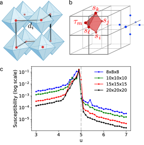
Figure 1: The dual lattice of the octahedral lattice is a cubic lattice, where the vertex model is defined (a). The spin model in (b) has the gauge symmetries indicated by the blue dots and the 5-spin interaction indicated by the red pyramids. Monte Carlo simulations of the dimer susceptibility suggest a transition at $u=5$.

Equivalent spin models— To understand the phase diagram better, we now study the statistical mechanics of the 3D classical vertex models by making use of a novel spin mapping. Recall that on the cubic lattice, with $V_{p}=6$, the vertex weights are $W_{6}(0)=W_{6}(6)=u$ and $W_{6}(2)=W_{6}(4)=1$. This vertex model has a $\mathbb{Z}_{2}$ gauge structure since the weights for odd vertices vanish. In order to make this more transparent, place spins on the plaquettes of the cubic lattice so that each link (corresponding to a dimer) is surrounded by four spins $s_{1},\cdots,s_{4}$. The dimer variable is mapped to spins as $d=s_{1}s_{2}s_{3}s_{4}$. One may surround a given vertex by a cube such that the spins lie on the edges of the cube; Fig. 1[b] shows the location of spins with respect to the cubic lattice built from these cubes. Our chosen encoding of dimer variables as spins automatically respects the even dimer constraint due to

$$\prod_{\square\in\mbox{\mancube}}s_{i}s_{j}s_{k}s_{\ell}=\prod_{-\in\mbox{\mancube}}s_{i}^{2}=1,$$ (7)

The term which enforces the even dimer constraint at a given vertex with the given vertex weights $W_{6}(n)$ is

$$W_{\mbox{\mancube}}(\vec{s})=\cosh\left(\mathcal{J}\sum_{\square\in\mbox{\mancube}}s_{i}s_{j}s_{k}s_{\ell}\right),$$ (8)

where $\frac{\cosh 6\mathcal{J}}{\cosh 2\mathcal{J}}=u$. The full partition function is therefore

$$\mathcal{Z}_{\text{spin}}=\sum_{\vec{s}\in\{-1,1\}^{N}}\prod_{\mbox{\mancube}}W_{\mbox{\mancube}}(\vec{s}).$$ (9)

One can convert the $\cosh$ to an exponential by adding a ghost spin $\tau$ at the center of each cube (i.e. on the vertices of the dual lattice); this gives the partition function

$$\mathcal{Z}_{\text{spin}}=\sum_{\vec{s},\vec{\tau}}\exp\left(\mathcal{J}\sum_{p}s_{i}s_{j}s_{k}s_{\ell}\tau_{m}\right),$$ (10)

where $p$ denotes the pyramid formed from the four spins surrounding a dimer and the ghost spin (see Figure 1[b]).

First note the standard $\mathbb{Z}_{2}$ gauge symmetry $P=\prod_{i\in v}X_{i}=X_{1}X_{2}X_{3}X_{4}X_{5}X_{6}$ is easily seen, where $X_{i}$ is the spin flip operator conjugate to $s_{i}$, and $i\in v$ denotes spins $s_{i}$ on the edges connected to site $v$ on the cubic lattice in Fig. 1[b] (shown as blue dots). Moreover, the gauge theory is enriched with a global $\mathbb{Z}_{2}$ symmetry due to the ghost spin $\tau_{p}$ placed on the tip of the pyramid $p$. This additional global symmetry is associated with two physical ground states (modulo gauge transformations) corresponding to $d_{i}=1,\tau_{i}=1$ and $d_{i}=-1,\tau_{i}=-1$. The global transformation $d_{i}\to-d_{i}$ requires flipping some subset of the $s$ spins (see Supplementary material for detail). As a result, an unusual aspect of this gauge theory is that it exhibits an “even-odd” behavior: the scaling of the Wilson loop $W_{C}=\left\langle\prod_{i\in C}s_{i}\right\rangle$ depends on whether $C$ encloses an even or an odd number of plaquettes, the latter being charged under the global $\mathbb{Z}_{2}$ symmetry. In the thermodynamic limit, both even and odd Wilson loops obey a perimeter law behavior at large $\mathcal{J}$, a consequence of simultaneous deconfinement and breaking of the global $\mathbb{Z}_{2}$ symmetry (see the Supplementary). Because the odd Wilson loop is charged under the global symmetry, it is zero in the small $\mathcal{J}$ limit while the even Wilson loop obeys an area law. Furthermore, since small odd Wilson loops correspond to local order parameters, the ordering transition is detected by odd Wilson loops of any size. As numerics indicate a single phase transition, both even and odd Wilson loops probe this transition.

On the diamond lattice, one can construct an analogous spin model by considering the dual pyrochlore lattice. We assign a spin to the center of each hexagon in the pyrochlore lattice; each spin $s_{\mathord{\raisebox{-1.0pt}{ \leavevmode\hbox to5.35pt{\vbox to4.69pt{\text{[drawing]}}}}}}$ is associated with the six corners of its hexagon, and each corner corresponds to the center of a dimer. Viewing the original pyrochlore lattice in terms of face sharing truncated tetrahedra $\mathcal{O}$, one of which is illustrated in Figure 2[b], the spins are sites of a dual pyrochlore lattice. We define the dimer variables $d_{c}=\prod_{\mathord{\raisebox{-1.0pt}{ \leavevmode\hbox to5.35pt{\vbox to4.69pt{\text{[drawing]}}}}}}s_{\mathord{\raisebox{-1.0pt}{ \leavevmode\hbox to5.35pt{\vbox to4.69pt{\text{[drawing]}}}}}}$ where the subscript denotes corner $c$ and the product is taken over the 6 hexagons which share $c$. The even dimer constraint is satisfied: $\prod_{c\in\raisebox{-1.0pt}{\includegraphics[height=6.02777pt]{tetrahedron.png}}}d_{c}=1$. It can also be seen that flipping the 4 spins associated with the 4 hexagons in truncated tetrahedron $\mathcal{O}$ via the operator $P=\prod_{\mathord{\raisebox{-1.0pt}{ \leavevmode\hbox to5.35pt{\vbox to4.69pt{\text{[drawing]}}}}}\in\mathcal{O}}X_{\mathord{\raisebox{-1.0pt}{ \leavevmode\hbox to5.35pt{\vbox to4.69pt{\text{[drawing]}}}}}}$ constitutes a gauge transformation.

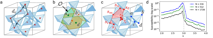
Figure 2: The dual of the pyrochlore lattice is the diamond lattice, where the vertex model is defined (a). The spins $s_{i}$ are placed on the centers of the hexagons forming a dual pyrochlore lattice, and the gauge symmetries are on objects $\mathcal{O}$ shown in (b). On the dual pyrochlore lattice, the gauge symmetry is on the tetrahedra and the 7-spin interaction is labelled in (c). Monte Carlo simulations of the dimer susceptibility show a phase transition around $u=3$ in (d) and $N$ denotes the number of sites in the simulation.

Thus, the term enforcing an 8-vertex configuration of spins is

$$W_{\raisebox{-1.0pt}{\includegraphics[height=6.02777pt]{tetrahedron.png}}}(\vec{s})=\cosh\left(\mathcal{J}\sum_{c\in\raisebox{-1.0pt}{\includegraphics[height=6.02777pt]{tetrahedron.png}}}(s_{1}s_{2}s_{3}s_{4}s_{5}s_{6})_{c}\right),$$ (11)

where $(s_{1}s_{2}s_{3}s_{4}s_{5}s_{6})_{c}$ denotes the product of 6 spins associated with corner $c$. The coupling $J$ satisfies $\cosh 4\mathcal{J}=u$. Introducing a ghost spin $\tau$, the partition function is

$$\mathcal{Z}_{\text{spin}}=\sum_{\vec{s},\vec{\tau}}\exp\left(\mathcal{J}\sum_{p}s_{i}s_{j}s_{k}s_{\ell}s_{m}s_{n}\tau_{r}\right),$$ (12)

with the 7-spin interaction on pyramid $p$ labelled in Figure 2[c]. On the dual pyrochlore lattice, construct dual truncated tetrahedra $\widetilde{\mathcal{O}}$; the ghost spins live on the centers of $\widetilde{\mathcal{O}}$. In terms of the original pyrochlore lattice, the ghost spins live on the centers of the tetrahedra, and thus form a diamond lattice. From an identical analysis to that of the octahedral spin liquid, the pyrochlore model possesses an even-odd effect with both even and odd Wilson loops detecting the same transition.

Now we ask how these order parameters are manifested in the original quantum spin model. For the cubic lattice model, the local order parameter from the odd Wilson loop corresponds to the dimer density which is an indicator of ferromagnetic order. In terms of the dimer variables, the non-local order parameter from the even Wilson loop in terms of dimer variables is $W_{\partial S}=\left\langle\prod_{i\in S}d_{i}\right\rangle$, where $\partial S$ is the boundary of an open surface. This is simply a ’t Hooft loop, which scales as a perimeter law in the confined phase and as an area law in the deconfined phase. The frustration-free models also admit a dual Wilson loop order parameter which is a product of $X_{i}$ along a loop of bonds [16]: $\widetilde{W}_{C}=\left\langle\prod_{i\in C}X_{i}\right\rangle$. All of these operators detect the same phase transition at the self dual point.

Effective field theories— We now proceed to characterizing the self dual points ($u=5$ for cubic and $u=3$ for diamond) by deriving an effective field theory. To do so, we observe that it is possible to introduce a new formulation of the vertex model in terms of height variables via the following exact rewriting of the partition function at the self dual point:

$$\mathcal{Z}_{0}=\int_{0}^{2\pi}d^{n}\theta\prod_{\langle p,q\rangle}\cos\left(\theta_{p}-\theta_{q}\right),$$ (13)

where $p$ and $q$ are sites on the diamond or cubic lattice. Interpreting $\theta_{p}$ as height fields, in the long wavelength limit, we assume that fluctuations of this field are small and can postulate a Euclidean field theory

$$\mathcal{Z}_{0}=\int\mathcal{D}\theta(x)\,\exp\left(-\frac{1}{2}\int d^{3}x\,(\nabla\theta)^{2}+\cdots\right),$$ (14)

which has an global $U(1)$ symmetry due to the shift invariance of $\theta$. A different height field representation was previously proposed for the 2D 8-vertex model on a square lattice [26, 27]. Since the decorated Wegner duality maps $u=3$ (or $u=5$) to an ice rule model on the corresponding lattice, we may verify this field theory by matching correlation functions to those in the ice rule model. The ice rule imposes a divergence-free constraint on electric field lines, so one can construct a vector potential and formulate an effective action [13]. Electric field correlations are equivalent to dimer correlations, which are dipolar in the ice rule limit: $\langle s_{i}(\bm{x})s_{j}(\bm{y})\rangle\sim\frac{1}{r^{5}}(3r_{i}r_{j}-r^{2}\delta_{ij})$, where $\bm{r}=\bm{y}-\bm{x}$. Under the decorated Wegner duality, one can show that this correlation function maps to

$$\frac{\int_{0}^{2\pi}d^{n}\theta\,\sin\left(\theta_{\bm{x}}-\theta_{\bm{x}+\bm{e_{i}}}\right)\sin\left(\theta_{\bm{y}}-\theta_{\bm{y}+\bm{e_{j}}}\right)\prod_{\langle p,q\rangle}\cos\left(\theta_{p}-\theta_{q}\right)}{\int_{0}^{2\pi}d^{n}\theta\prod_{\langle p,q\rangle}\cos\left(\theta_{p}-\theta_{q}\right)}.$$ (15)

where the product over $\langle p,q\rangle$ omits the two edges where the operators are located. Therefore, in the long wavelength limit $\langle s_{i}(\bm{x})s_{j}(\bm{y})\rangle$ is mapped to $\langle\partial_{i}\theta(\bm{x})\partial_{j}\theta(\bm{y})\rangle$, which in our postulated field theory has a dipolar form. Next, we inquire what the spontaneous dimer density is near the critical point. The operator $\langle d_{i}(\bm{x})d_{j}(\bm{y})\rangle$ can be shown to be written as

$$\frac{\int_{0}^{2\pi}d^{n}\theta\,\cos\left(\theta_{\bm{x}}+\theta_{\bm{x}+\bm{e_{i}}}\right)\cos\left(\theta_{\bm{y}}+\theta_{\bm{y}+\bm{e_{j}}}\right)\prod_{\langle p,q\rangle}\cos\left(\theta_{p}-\theta_{q}\right)}{\int_{0}^{2\pi}d^{n}\theta\prod_{\langle p,q\rangle}\cos\left(\theta_{p}-\theta_{q}\right)}$$ (16)

which maps onto $\langle\cos(2\theta(\bm{x}))\cos(2\theta(\bm{y}))\rangle$ in the long-wavelength limit. In $d\geq 3$, this operator exhibits long range order in our postulated field theory. Thus, in the dimer variables, the self dual point exhibits a first order transition. We may also consider the operator $\langle\sin(2\theta(\bm{x}))\sin(2\theta(\bm{y}))\rangle$, which corresponds to applying two test charges and computing the ratio of partition functions with and without the charges; this operator is thus a diagnostic for deconfinement. Since this operator also exhibits long range order when $d\geq 3$, at the transition point one local order and deconfinement coexist.

Next, we discuss what occurs when one perturbs about the self dual point. We utilize the following exact rewriting of the partition function

$$\mathcal{Z}_{\alpha}=\int_{0}^{2\pi}d^{n}\theta\prod_{\langle p,q\rangle}\left(f(\theta_{p})f(\theta_{q})+g(\theta_{p})g(\theta_{q})\right),$$ (17)

where $f(\theta)=\cos\theta+\alpha\cos(3\theta)$ and $g(\theta)=\sin\theta-\alpha\sin(3\theta)$. In the diamond lattice, we find that

$$u(\alpha)=3+\frac{16\alpha}{\alpha^{4}+4\alpha^{2}-4\alpha+1}$$ (18)

and a similar expression can be found on the cubic lattice. Thus, for small positive values of $\alpha$, the vertex model is perturbed into the ordered phase, while for small negative values of $\alpha$, the vertex model is perturbed into the disordered phase. The partition function, using the explicit forms for $f$ and $g$, can be simplified to

$$\mathcal{Z}_{\alpha}=\int_{0}^{2\pi}d^{n}\theta\prod_{\langle p,q\rangle} \biggl{(}\cos(\theta_{p}-\theta_{q})+\alpha^{2}\cos(3\theta_{p}-3\theta_{q})$$

$$+\alpha\cos(3\theta_{p}+\theta_{q})+\alpha\cos(3\theta_{q}+\theta_{p})\biggr{)},$$

which in the long wavelength limit, assuming we can expand the cosine angle differences, becomes a sine-Gordon model to leading order in $\alpha$:

$$\mathcal{Z}_{\alpha}=\int\mathcal{D}\theta(x)\,\exp\left(-\frac{1}{2}\int d^{3}x\,(\nabla\theta)^{2}-4\alpha\cos(4\theta)+\cdots\right)$$ (19)

There are a couple of features we see immediately. First, at $\alpha=0$ the $U(1)$ symmetry implies that all symmetry breaking cosine terms vanish. Next, because we are in 3+0D, the instanton term is RG relevant by Polyakov’s argument [28], which is equivalent to the fact that the symmetry breaking terms above are relevant. Thus the self dual point indeed indicates a transition, consistent with numerics. For small positive $\alpha$, we find a smooth phase where $\langle\cos(4\theta)\rangle=1$, which corresponds to $|\langle\cos(2\theta)\rangle|=1$, or a ferromagnetically ordered phase. For small negative $\alpha$, we find another smooth phase where $\langle\cos(4\theta)\rangle=-1$; since $\langle\cos(2\theta)\rangle=0$, this corresponds to a disordered phase in the dimer density variables. Both the ordered and disordered phases are massive and therefore gapped. The operator $|\langle\sin(2\theta)\rangle|$ is $0$ when $\alpha$ is positive and $1$ when $\alpha$ is negative, and is thus an indicator of topological order. Under Wegner’s duality, appropriately dressed versions of the operators $\cos(2\theta)$ and $\sin(2\theta)$ are swapped (see Supplementary material for a derivation). Phenomenologically, we could arrive at the same action by writing down terms consistent with invariance under the $\mathbb{Z}_{2}$ symmetry $\cos(2\theta)\to-\cos(2\theta)$:

$$\mathcal{S}=\int d^{3}x\,\left(\frac{1}{2}(\nabla\theta)^{2}+\cdots+\sum_{n}c_{n}\cos(4n\theta)\right).$$ (20)

Furthermore, in the original spin model, the local dimer density at each vertex is bounded between $-V_{p}$ and $+V_{p}$. As the operator $\cos(4n\theta)$ corresponds to changing the relative weight of vertex configurations with $k$ and $k\pm 4n$ dimers at a fixed site, we require $4n\leq V_{p}$, which gives the proposed action for $V_{p}=4,6$.

We now discuss the implications of this transition point when quantum fluctuations are added to perturb away from the RK point. Consider extending the microscopic Hamiltonian (on the diamond lattice, an identical result holds for the cubic lattice) in Eqn. 6 beyond the RK point, via some generic isotropic perturbation of strength $\delta$. Because we know the effective field theory describing the RK wavefunction is Gaussian, a well-known result is that the effective field theory for the Hamiltonian as a function of a perturbation $J$ near $u=3$ is a quantum Lifshitz model [29, 30, 31, 16, 2], with the imaginary time action

$$\mathcal{S}=\int d^{3}x\,d\tau\,\left(\frac{1}{2}(\partial_{\tau}\theta)^{2}+\frac{\kappa}{2}(\nabla^{2}\theta)^{2}+\delta(\nabla\theta)^{2}\right)+\mathcal{S}_{\text{inst}},$$ (21)

where $\delta$ measures the deviation from the RK point, and $\mathcal{S}_{\text{inst}}$ accounts for instanton events: $\mathcal{S}_{\text{inst}}=\int d^{3}x\,d\tau\,g\cos(4\theta)$ [2]. We have studied the RK point when $\delta=0$, but when $\delta>0$, the $(\nabla^{2}\theta)^{2}$ term is RG irrelevant while the instanton term is still strongly RG relevant. Thus, the RK transition point at $u=3$ turns into a line of first order phase transitions between the $\mathbb{Z}_{2}$ deconfined and ferromagnetic phases. An example of a perturbation that might correspond to increasing $\delta$ is tuning away from $J=0$ in Eqn. 6. Notably, at $u=1$ the Hamiltonian is always a sum of commuting projectors regardless of the value of $J$, which only contributes to a global shift of the energy. Thus for this choice of perturbation the first order line will never merge into the $U(1)$ phase near $u=0$.

Finally, we address the fate of the coexistence of ferromagnetic order and deconfinement at the transition point as we move along the first order line, corresponding to fixing $g=0$. This requires us to compute the equal-time correlators $\langle\cos(2\theta(\bm{x}))\cos(2\theta(\bm{y}))\rangle$ and $\langle\sin(2\theta(\bm{x}))\sin(2\theta(\bm{y}))\rangle$ for small, positive $\delta$ in the quantum Lifshitz theory. In the long wavelength limit, $\kappa(\nabla^{2}\theta)^{2}$ is RG irrelevant at small positive $\delta$ and we can ignore it. Noting that

$$\langle\cos(2\theta(\bm{x}))\cos(2\theta(\bm{y}))\rangle=\frac{1}{2}\exp\left(2\langle\theta(\bm{x})\theta(\bm{y})\rangle\right)$$ (22)

and similarly for the sine correlator, we find that $\langle\theta(\bm{x})\theta(\bm{y})\rangle\sim|\bm{x}-\bm{y}|^{-1}$, and therefore both correlators exhibit long range order along the first order line, indicating that coexistence indeed persists.

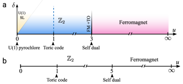
Figure 3: Panel (a) $u$-axis (where $u$ is the vertex weight) and panel (b) show the phase diagram of the frustration free models, whose ground states are given by classical vertex models on the diamond and cubic lattices respectively. The $\delta$-axis in panel (a) shows a possible phase diagram (to leading order in $u-u^{*}$, where $u^{*}$ is the self dual point) of the diamond lattice model upon moving away from the RK line.

Acknowledgements – A.V. and V. G. were supported by the Simons Collaboration on Ultra Quantum Matter, a grant from the Simons Foundation (651440, A.V.). S.B. was supported by the National Science Foundation Graduate Research Fellowship under Grant No. 1745302. V.G. was also supported by NSF DMR-2037158 and US-ARO Contract No.W911NF1310172. D.B. was supported by JQI-PFC-UMD.

Appendix A Vertex models and Wegner’s duality

In this section, we review known results of duality mappings for vertex models, with an emphasis on the dimensionality independence of the results. Part of this appendix serves as a summary of [20]. We first will derive Wegner’s duality for vertex models on a generic lattice. To start, consider a vertex model on the dual lattice $G$. We define spin variables $s_{pq}$ located on the edges of $G$, and we will assume that the vertex weights are only a function of the total number of bonds $b$ coming out of a site and are labelled as $W(b)$. If $s_{pq}=1$, then $\langle p,q\rangle$ forms an occupied bond on the vertex model. Then, the partition function of the vertex model can be written as

$$\mathcal{Z}=\sum_{\vec{s}\in\{-1,1\}^{N}}\prod_{p\in G}\sum_{b=0}^{V_{p}}\delta\left(S_{\text{tot}}(p)=2b-V_{p}\right)W_{p}(b),$$ (23)

where $S_{\text{tot}}(p)=\sum_{(p,q)\in G}s_{pq}$. We perform a Fourier transform of the $\delta$-functions using the relation

$$\delta\left(\sum_{i\in p}s_{i}=c\right)=\frac{1}{2\pi}\int_{0}^{2\pi}d\theta_{p}\,e^{i\theta_{p}\left(\sum_{i\in p}s_{i}-c\right)},$$ (24)

and we may rearrange the partition function upon inserting this identity to obtain

$$\mathcal{Z}=\frac{1}{(2\pi)^{n}}\int_{0}^{2\pi}d^{n}\theta\sum_{\vec{s}\in\{-1,1\}^{N}}\prod_{(q,\ell)\in G_{D}}e^{is_{q\ell}(\theta_{q}+\theta_{\ell})}$$

$$\times\prod_{p\in G_{D}}\sum_{b=0}^{V_{p}}e^{-i\theta_{p}(2b-V_{p})}W_{p}(b).$$ (25)

Performing the sum over spins, we find

$$\mathcal{Z}=\frac{2^{N}}{(2\pi)^{n}}\int_{0}^{2\pi}d^{n}\theta\prod_{(q,\ell)\in G_{D}}\cos(\theta_{q}+\theta_{\ell})$$

$$\times\prod_{p\in G_{D}}\sum_{b=0}^{V_{p}}e^{-i\theta_{p}(2b-V_{p})}W_{p}(b).$$ (26)

Next, expand the cosine using $\cos(\theta_{q}+\theta_{\ell})=\cos\theta_{q}\cos\theta_{\ell}-\sin\theta_{q}\sin\theta_{\ell}$, and associate no bond with a factor of $\cos\theta_{q}\cos\theta_{\ell}$ and a bond with a factor of $-\sin\theta_{q}\sin\theta_{\ell}$. Performing this expansion and regrouping terms maps the partition function to

$$\mathcal{Z}=\sum_{k_{1},k_{2},\cdots,k_{n}}\frac{2^{N}}{(2\pi)^{n}}\int_{0}^{2\pi}d^{n}\theta\prod_{p\in G_{D}}\sum_{b=0}^{V_{p}}i^{V_{p}-k_{p}}\cos^{k_{p}}\theta_{p}\sin^{V_{p}-k_{p}}\theta_{p}e^{-i\theta_{p}(2b-V_{p})}W_{p}(b),$$ (27)

which can be written in the compact form

$$\mathcal{Z}=\sum_{k_{1},k_{2},\cdots,k_{n}}\prod_{p}W^{\prime}_{p}(k_{p}),$$ (28)

where

$$W^{\prime}_{p}(k_{p})=\sum_{b=0}^{V_{p}}i^{V_{p}-k_{p}}\left\langle\cos^{k_{p}}\theta_{p}\sin^{V_{p}-k_{p}}\theta_{p}e^{-i\theta_{p}(2b-V_{p})}\right\rangle W_{p}(b).$$ (29)

Here, the notation $\langle f(\theta)\rangle=\frac{1}{2\pi}\int_{0}^{2\pi}f(\theta)\,d\theta$. This defines a new vertex model precisely with weights $W^{\prime}$. The new weights are related to the old weights by the linear map $\mathcal{M}\colon W_{p}\to W^{\prime}_{p}$, which is defined on the space of vertex weights. The matrix $\mathcal{M}$ has elements

$$\mathcal{M}_{ab}=i^{V_{p}-a}\left\langle\cos^{a}\theta_{p}\sin^{V_{p}-a}\theta_{p}e^{-i\theta_{p}(2b-V_{p})}\right\rangle.$$ (30)

$\mathcal{M}$ can be divided into disjoint eigenspaces corresponding to each of its distinct eigenvalues. Any configuration of vertex weights which lives entirely in a given eigenspace will remain in the eigenspace under the application of $\mathcal{M}$. Therefore, these eigenspaces define a self-dual manifold; if a parameterization of a vertex model pierces the self-dual manifold and exhibits a single phase transition, then the transition point occurs at the intersection with the self-dual manifold. An example of $\mathcal{M}_{ab}$ for $V_{p}=6$ is

$$\mathcal{M}_{ab}=\begin{pmatrix}\frac{1}{8}&-\frac{3}{4}&\frac{15}{8}&-\frac{5}{2}&\frac{15}{8}&-\frac{3}{4}&\frac{1}{8}\\ -\frac{1}{8}&\frac{1}{2}&-\frac{5}{8}&0&\frac{5}{8}&-\frac{1}{2}&\frac{1}{8}\\ \frac{1}{8}&-\frac{1}{4}&-\frac{1}{8}&\frac{1}{2}&-\frac{1}{8}&-\frac{1}{4}&\frac{1}{8}\\ -\frac{1}{8}&0&\frac{3}{8}&0&-\frac{3}{8}&0&\frac{1}{8}\\ \frac{1}{8}&\frac{1}{4}&-\frac{1}{8}&-\frac{1}{2}&-\frac{1}{8}&\frac{1}{4}&\frac{1}{8}\\ -\frac{1}{8}&-\frac{1}{2}&-\frac{5}{8}&0&\frac{5}{8}&\frac{1}{2}&\frac{1}{8}\\ \frac{1}{8}&\frac{3}{4}&\frac{15}{8}&\frac{5}{2}&\frac{15}{8}&\frac{3}{4}&\frac{1}{8}\\ \end{pmatrix},$$ (31)

and explicitly, it can be seen that the eigenvalues of $\mathcal{M}_{ab}$ are $\pm 1$. The eigenspaces corresponding to these eigenvalues are

$$\mathcal{V}_{-1}=\text{span}\left\{\begin{pmatrix}-4\\ 0\\ 1\\ -1\\ 0\\ 0\\ 1\end{pmatrix},\begin{pmatrix}-12\\ 1\\ 4\\ -3\\ 0\\ 1\\ 0\end{pmatrix},\begin{pmatrix}-15\\ 0\\ 4\\ -3\\ 1\\ 0\\ 0\end{pmatrix}\right\}$$ (32)

and

$$\mathcal{V}_{1}=\text{span}\left\{\begin{pmatrix}4\\ -2\\ 1\\ 0\\ 0\\ 0\\ 1\end{pmatrix},\begin{pmatrix}0\\ -1\\ 0\\ 0\\ 0\\ 1\\ 0\end{pmatrix},\begin{pmatrix}-15\\ 10\\ -4\\ 0\\ 1\\ 0\\ 0\end{pmatrix},\begin{pmatrix}-20\\ 10\\ -4\\ 1\\ 0\\ 0\\ 0\end{pmatrix}\right\}.$$ (33)

The vector $W_{p}(k)=\langle\cos^{k}\theta\sin^{V_{p}-k}\theta\rangle$, or $\langle 5,0,1,0,1,0,5\rangle$ explicitly, lies in the $\mathcal{V}_{1}$ eigenspace, which we have argued in the text corresponds to a self-dual point. However, what we point out here is that this is a self-dual point on any 32-vertex model defined on a 6-coordinated lattice in any dimension. In a previous paper [20], we showed in general that the vertex weights

$$W_{p}(k)=\langle\cos^{k}\theta\sin^{V_{p}-k}\theta\rangle$$ (34)

are a self-dual point for a vertex model defined on a $V_{p}$-coordinated lattice in any dimension.

The decorated Wegner duality can be seen by composing the Wegner duality with the mapping $u\to-u$. We will highlight an explicit example of the decorated Wegner duality by showing that an arrowed vertex model satisfying an ice rule on lattice $G$ maps onto the critical point of the vertex model on lattice $G$ with weights given in Eqn. 34. To see this, place an additional site on each edge, which will have degree $V_{p}=2$. Placing spins on the edges of this new lattice, the arrowed ice rule model thus satisfies the constraint that the total spin around each site equals zero. Under Wegner’s duality, we find the vertex weights

$$W_{p}(k)=i^{V_{p}-k}\langle\cos^{k}\theta\sin^{V_{p}-k}\theta\rangle.$$ (35)

Eliminating sites with coordination number 2, the vertex weights must be modified by weighting each dimer by an additional factor of $-1$; this recovers the vertex weights in Eqn. 34. If $G$ was originally bipartite, the additional sites do not need to be added, and arrows can be converted to bonds without changing the physics. Such is the case for the diamond and cubic lattice models.

Appendix B Height field theory for vertex models

With the representation from Eqn. 34 in mind, it is possible to verify the claim that the partition function at the self-dual point can be written as

$$\mathcal{Z}\propto\int_{0}^{2\pi}d^{n}\theta\prod_{\langle p,q\rangle}\cos\left(\theta_{p}-\theta_{q}\right)$$ (36)

by expanding the cosine term and regrouping. With nonzero $\alpha$, the vertex weights are

$$W_{p}(k)=\langle(\cos\theta+\alpha\cos 3\theta)^{k}(\sin\theta-\alpha\sin 3\theta)^{V_{p}-k}\rangle$$ (37)

which reproduces the formula for the diamond lattice. For the cubic lattice with $V_{p}=6$, we find

$$u(\alpha)=5+\frac{40\alpha(1+2\alpha^{2})}{\alpha^{6}+9\alpha^{4}-10\alpha^{3}+9\alpha^{2}-5\alpha+1}.$$ (38)

For lattices with $V_{p}>6$, other perturbations can be achieved by trying

$$W_{p}(k)=\langle(\cos\theta+\alpha\cos n\theta)^{k}(\sin\theta-\alpha\sin n\theta)^{V_{p}-k}\rangle$$ (39)

for other choices of $n\in 4\mathbb{Z}-1$. In 3+0D, we suspect that because instanton terms are relevant for any value of $n$, the choice of weights above can be the only possible gapless point. However, in 2+0D, for sufficiently large $n$, instanton terms are irrelevant, which may open the possibility to gapless lines, planes, and beyond.

Appendix C Proof that dimer density and deconfinement diagnostics swap

First, it is easy to see what the dimer density operator is in terms of the $\theta$ fields: simply replacing $\cos\left(\theta_{p}-\theta_{q}\right)$ with $\cos\left(\theta_{p}+\theta_{q}\right)$ will add a relative weight of $-1$ between dimer and no dimer configurations upon expanding the cosine, thus computing the dimer density.

Next, we proceed to show that under Wegner’s duality, the dimer density and deconfinement diagnostics swap. We can make this explicit at the self dual point. First we compute the dimer-dimer correlator:

$$\langle d_{p_{1}q_{1}}d_{p_{2}q_{2}}\rangle=\frac{1}{Z} \sum_{\vec{s}\in\{-1,1\}^{N}}s_{p_{1}q_{1}}s_{p_{2}q_{2}}\cdot$$

$$\prod_{p\in G}\sum_{b=0}^{V_{p}}\delta\left(S_{\text{tot}}(p)=2b-V_{p}\right)W_{p}(b).$$ (40)

Expanding the $\delta$-functions as before gives the expression

$$\langle d_{p_{1}q_{1}}d_{p_{2}q_{2}}\rangle\propto\frac{1}{\mathcal{Z}}\int_{0}^{2\pi}d^{n}\theta\,\sin(\theta_{p_{1}}+\theta_{q_{1}})\sin(\theta_{p_{2}}+\theta_{q_{2}})$$

$$\times\prod_{(q,\ell)\in G_{D}}\cos(\theta_{q}+\theta_{\ell})\prod_{p\in G_{D}}\sum_{b=0}^{V_{p}}e^{-i\theta_{p}(2b-V_{p})}W_{p}(b).$$ (41)

where the notation $(q,\ell)\in G_{D}$ ignores the two edges $\langle p_{1},q_{1}\rangle$ and $\langle p_{2},q_{2}\rangle$. We proceed by identifying a dimer coming into a vertex with a factor $i\sin\theta$ at that vertex, and no dimer with a factor of $\cos\theta$. However, only at nodes $p_{1}$ and $p_{2}$, the notion of dimer and no dimer are reversed for the edges $\langle p_{1},q_{1}\rangle$ and $\langle p_{2},q_{2}\rangle$. Therefore, under Wegner’s duality, the dual vertex weights are $W_{p}(k)=\langle\cos^{k}\theta\sin^{V_{p}-k}\theta\rangle$ for all nodes not equal to $p_{1}$ and $p_{2}$. At $p_{1}$ and $p_{2}$, the vertex weights are

$$\widetilde{W}_{p}(k,m)=\langle\cos^{k+m}\theta\sin^{V_{p}-k-m}\theta\rangle,$$ (42)

where $m=\pm 1$ denotes whether the corresponding special edge has a dimer ($-1$) or not ($+1$). In particular, this forces $k$ to be odd, and therefore these sites are defected. It can then be seen that the quantity

$$\frac{1}{\mathcal{Z}}\int_{0}^{2\pi}d^{n}\theta\,\sin(\theta_{p_{1}}+\theta_{q_{1}})\sin(\theta_{p_{2}}+\theta_{q_{2}})\prod_{\langle p,q\rangle}\cos\left(\theta_{p}-\theta_{q}\right)$$ (43)

precisely gives the same vertex weights. In the continuum, this turns into $\langle\sin(2\theta_{1})\sin(2\theta_{2})\rangle$, as desired. Note that away from the critical point, the dimer density operator gets deformed by a correction of order $\alpha$, and so the identification $\cos 2\theta\leftrightarrow\sin 2\theta$ is correct to zeroth order. Computing the full form of the dimer density and the dual deconfinement parameter can be done but is not important for us.

Appendix D Equivalence of decorated Wegner duality and pure gauge theory – XY model duality

From the field theory perspective, the mapping from an ice rule model onto the self dual point ($u=0$ to $u=3$ in the case of the diamond lattice) is a consequence of the well-known mapping from a pure gauge theory to an XY model. In particular, in 3+0D, the ice rule constraint enforces a divergence-free constraint on the electric field lines. In the path integral representation, this can be written as

$$\mathcal{Z}=\int\mathcal{D}\bm{E}\,\exp\left(-\frac{1}{2}\int d^{3}x\,\bm{E}^{2}\right)\delta(\nabla\cdot\bm{E}=0).$$ (44)

Writing the $\delta$-function in terms of a Lagrange multiplier, we find that

$$\mathcal{Z}=\int\mathcal{D}\bm{E}\,\mathcal{D}\theta\,\exp\left(-\frac{1}{2}\int d^{3}x\,\bm{E}^{2}-i\theta(\nabla\cdot\bm{E})\right),$$ (45)

and integrating over $\bm{E}$ maps us precisely onto the proposed action for the height fields $\theta$. A similar analysis can be done in 2+1D by defining $\bm{E}$ in terms of electric and magnetic fields so that the divergence-free constraint is equivalent to Faraday’s law.

The field-theoretic argument above shows that the height field representation of the self-dual point is a generic feature of any vertex model defined on a lattice. So long as the lattice is regular and isotropic, we believe that the critical point with vertex weights $W_{p}(k)=\langle\cos^{k}\theta\sin^{V_{p}-k}\theta\rangle$ is a Gaussian fixed point where deconfinement and local order coexist in $d\geq 3$.

Appendix E Matching degrees of freedom in spin and vertex models

We show explicitly the correctness of the dimer model to spin model mapping presented in the main text by arguing that each dimer configuration is uniquely mapped to a spin configuration. This can be shown by matching dimer and spin degrees of freedom through a counting argument.

We first work with the cubic lattice spin model, where

$$\mathcal{Z}_{\text{spin}}=\sum_{\vec{s}\in\{-1,1\}^{N}}\prod_{\mbox{\mancube}}W_{\mbox{\mancube}}(\vec{s}).$$ (46)

First note the standard $\mathbb{Z}_{2}$ gauge symmetry $P=\prod_{i\in v}X_{i}=X_{1}X_{2}X_{3}X_{4}X_{5}X_{6}$ where $X_{i}$ is the spin flip operator, and $i\in v$ denotes spins on the edges connected to vertex $v$. Therefore, the number of gauge equivalent spin configurations is $2^{N}$, where $N$ is the number of lattice sites in the lattice. The number of valid 32-vertex configurations $D$ is $2^{2N}$ for any lattice with coordination number 6. If each dimer configuration corresponds to $2^{N}$ spin configurations, then there must be a total of $D\cdot 2^{N}=2^{3N}$ spin configurations, which coincides with the number of spin degrees of freedom in the dual spin model (as spins are defined on the edges of the cubic lattice). Therefore, the dimer model and spin model partition functions are related by $\mathcal{Z}_{\text{spin}}(J)=2^{N}\mathcal{Z}_{\text{dimer}}(J)$.

Next, we show that the partition function for the 7-spin model maps to the partition function of the vertex model for the diamond lattice model. The number of valid vertex model configurations on the diamond lattice is $D=2^{N_{T}}$, where $N_{T}$ is the number of tetrahedra in the dual pyrochlore lattice. The number of objects $\mathcal{O}$ (see main text) is $N_{T}$ and each object $\mathcal{O}$ is associated with a local gauge transformation. The total number of spin degrees of freedom is therefore $D\cdot 2^{N_{T}}=2^{2N_{T}}=2^{N_{H}}$ where $N_{H}$ is the number of hexagons; this coincides with the number of degrees of freedom in the above spin model. Therefore $\mathcal{Z}_{\text{spin}}(J)=2^{N_{T}}\mathcal{Z}_{\text{dimer}}(J)$.

Appendix F Global symmetry $\tau_{i}\to-\tau_{i}$ and $d_{i}\to-d_{i}$ in cubic lattice model

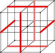
Figure 4: The configuration of spins that must be flipped to implement the global symmetry transformation. The bond spins live on the links of the lattice.

In the main text, we noted that the equivalent spin model possesses a global symmetry corresponding to $\tau\to-\tau$ and $d\to-d$. It is not immediately obvious if there exists a transformation on the bond spins $s$ such that $d\to-d$. We show this transformation in Figure 4. The red bonds indicate that the associated spins are flipped, and the structure of red bonds is repeated over the entire lattice.

Appendix G Even-odd effect for cubic lattice model

(In this section we will change variables from $\mathcal{J}$ to $\beta$ for clarity). We will discuss the phases of the gauge theory and the even-odd effect. We start with the Hamiltonian for the cubic lattice spin model, Equation 10. Consider the Wilson loop operator

$$W_{C}=\left\langle\prod_{i\in C}s_{i}\right\rangle,$$ (47)

where $C$ is a closed loop containing the gauge spins. Let us first analyze this quantity at low temperatures, in the deconfined phase. Here, the standard analysis holds, which we review for convenience [32]. We gauge fix so that the ground state spin configuration is the ferromagnetic configuration. We then proceed with a low temperature expansion: flipping a gauge spin will negate 8 plaquette terms, while flipping a ghost spin will negate 6 plaquette terms. Therefore, the first order correction to the Wilson surface is

$$\left\langle\prod_{i\in\partial V}s_{i}\right\rangle =\frac{\sum_{\vec{s}}\left(\prod_{i\in\partial V}s_{i}\right)e^{-\beta H(\vec{s})}}{\sum_{\vec{s}}e^{-\beta H(\vec{s})}}$$

$$=\frac{1+(N-2L)e^{-16\beta}+Ne^{-12\beta}+\cdots}{1+Ne^{-16\beta}+Ne^{-12\beta}+\cdots}$$ (48)

where $L$ is the length of the loop. For $n$ spin flips, we make the assumption that they are independent. Then, the contribution $F(n)$ to the numerator is

$$F(n)=\sum_{a+b=n}\frac{(N-2L)^{a}}{a\,!}\frac{N^{b}}{b\,!}e^{-\beta(16a+12b)}$$ (49)

and the contribution to the denominator $G(n)$ is

$$G(n)=\sum_{a+b=n}\frac{N^{a}}{a\,!}\frac{N^{b}}{b\,!}e^{-\beta(16a+12b)}.$$ (50)

Then, the Wilson surface roughly has the expectation value

$$\left\langle\prod_{i\in\partial V}s_{i}\right\rangle \approx\frac{1+F(1)+F(2)+\cdots}{1+G(1)+G(2)+\cdots}$$

$$=\frac{\exp\left((N-2L)e^{-16\beta}+Ne^{-12\beta}\right)}{\exp\left(Ne^{-16\beta}+Ne^{-12\beta}\right)}$$

$$=\exp\left(-2L\cdot e^{-16\beta}\right),$$ (51)

which is representative of the deconfined phase.

Next, we understand what happens in the confined phase. For this, we need to perform a high temperature expansion of the partition function:

$$\mathcal{Z}=\left(\cosh\beta\right)^{N}\sum_{\vec{s}}\prod_{p}(1+\tanh\beta\,(s_{i}s_{j}s_{k}s_{\ell}\tau_{m})).$$ (52)

and the Wilson loop looks like

$$\left\langle\prod_{i\in C}s_{i}\right\rangle=\frac{\sum_{\vec{s}}\left(\prod_{i\in\partial V}s_{i}\right)\prod_{p}(1+\tanh\beta\,(s_{i}s_{j}s_{k}s_{\ell}\tau_{m}))}{\sum_{\vec{s}}\prod_{p}(1+\tanh\beta\,(s_{i}s_{j}s_{k}s_{\ell}\tau_{m}))}.$$ (53)

Naively, in analogy to the Ising gauge theory, one may fill the interior of $C$ with plaquettes. Doing this results in $A$ dangling ghost spins, where $A$ is the area of the loop. These ghost spins are sites on a 2D square lattice with boundary $C$. Next, we may rewrite a correlation function of two ghost spins as

$$\tau_{i}\tau_{j}=\prod_{k=i}^{j}\tau_{k}\left(\prod_{\alpha\in\square_{k}}s_{\alpha}\right)^{2}\tau_{k+1}$$ (54)

where the first product $\prod_{k=i}^{j}$ is over a string connecting $i$ and $j$ and the second product $\prod_{\alpha\in\square_{k}}s_{\alpha}$ is over bond spins on the plaquette adjacent to ghost spin $\tau_{k}$ and pointing out of the plane of ghost spins. This identity may be written as a product of a string of pyramidal operators connecting $\tau_{i}$ and $\tau_{j}$. To satisfy each ghost spin in the 2D substructure, we need to connect pairs of them together via strings of pyramidal operators while minimizing the total number of pyramidal operators. The way to do this is for the string operators to mimic dimer configurations on the square lattice. There are 2 pyramids involved per dimer, and therefore $A$ pyramids involved in a given dimer configuration. Then, the leading order contribution to the Wilson operator looks like

$$\left\langle\prod_{i\in C}s_{i}\right\rangle\sim\left(\tanh\beta\right)^{A}\cdot D_{S}\left(\tanh\beta\right)^{A}+\cdots,$$ (55)

where $D_{S}$ is the number of dimer configurations on the square lattice with $A$ sites,

$$\lim_{A\to\infty}\frac{1}{A}\log D_{S}=\frac{2G}{\pi},$$ (56)

and $G$ is Catalan’s constant. Therefore, the Wilson surface obeys an area law in the confined phase for large enough temperatures.

If the Wilson loop encloses an odd number of plaquettes, then filling the interior or any extrusion of the loop with plaquettes will result in an odd number of dangling ghost spins. These cannot be paired together without excluding a single ghost spin. This single ghost spin can only be resolved by a string of pyramids connecting the ghost spin to the boundary of the lattice. The Wilson loop then behaves like

$$\left\langle\prod_{i\in C}s_{i}\right\rangle\lesssim D_{S}\left(\tanh^{2}\beta\right)^{A}\cdot(6\tanh\beta)^{\sqrt[3]{N}}+\cdots,$$ (57)

which for small enough $\beta$ vanishes in the thermodynamic limit $N\to\infty$.

Appendix H Simulation details

The Monte Carlo simulation consisted of loop moves implemented as Metropolis updates. While the plot shown in the main text provides convincing evidence for a transition at $u=5$ for the octahedral lattice, here we provide further plots to corroborate this. In particular, we plot the magnetization as a function of the number of samples (which is proportional to the total number of updates). We see that the transition point indeed robustly converges to $u=5$. The results are shown in Fig. 5.

Figure 5: The Monte Carlo results show that as the number of samples increases, the transition point converges to the self dual point at $u=5$. The magnetization per spin is plotted. Similar plots were generated for the heat capacity, which indicates that there is a single unique transition.

Appendix I Simple proof of spontaneously magnetized phase

We present a short and rigorous proof that the symmetry enriched $\mathbb{Z}_{2}$ gauge theory for the cubic lattice model exhibits a phase transition in the local order parameter, and will thus arrive at a bound on the transition temperature (even though in the text, the transition temperature is computed exactly). To do this, we will rely on the Griffiths-Kelly-Sherman inequalities, which state that for a classical spin model with purely ferromagnetic multispin interactions $J_{1},J_{2},\cdots$, the expectation value of a product of spin operators, $\mathcal{O}=\prod_{i\in S}s_{i}$ where $S$ is some set, satisfies

$$\frac{\partial\langle\mathcal{O}(J_{1},J_{2},\cdots)\rangle}{\partial J_{i}}\geq 0.$$ (58)

In particular, for the 5-spin interaction model, we remove pyramidal interactions everywhere except for a two-dimensional layer of cubes. We then remove the pyramids on the top and the bottom of each cube, and as a result, we know that the magnetization can only decrease as a result of removing all of these interactions. The corresponding classical spin Hamiltonian will then take the form

$$\mathcal{H}=J\sum_{p^{\prime}}s_{1}s_{2}s_{3}s_{4}\tau_{5}$$ (59)

where the ^′ symbol indicates the sum is only over the remaining pyramids. Among the 4 bond spins $s_{1}$, $s_{2}$, $s_{3}$, and $s_{4}$, two spins are shared by two pyramids, while the other two spins are shared by four pyramids. If we call the former spins $\overline{s}$, then

$$\sum_{\overline{s}}\exp\left(J\sum_{p^{\prime}}\overline{s}_{1}\overline{s}_{2}s_{3}s_{4}\tau_{5}\right)\propto\prod_{\langle p,q\rangle}\cosh\left(Js_{3}s_{4}(\tau_{p}+\tau_{q})\right)$$ (60)

where $\langle p,q\rangle$ correspond to edges in the square lattice formed by the sites of the ghost spins. Through the standard trick

$$\sum_{s_{3},s_{4}}\cosh\left(Js_{3}s_{4}(\tau_{p}+\tau_{q})\right)=2\cosh\left(J(\tau_{p}+\tau_{q})\right)$$ (61)

and the identity

$$2\cosh\left(J(\tau_{p}+\tau_{q})\right)=1-\tau_{p}\tau_{q}+(1+\tau_{p}\tau_{q})\cosh 2J$$ (62)

The partition function becomes

$$\mathcal{Z}\propto\sum_{\tau}\exp\left(J^{\prime}\sum_{\langle p,q\rangle}\tau_{p}\tau_{q}\right),$$ (63)

where

$$\tanh J^{\prime}=\frac{\cosh 2J-1}{\cosh 2J+1}.$$ (64)

In 2D, we know that the Ising model spontaneously magnetizes, and since the magnetization in the 5-spin model has a strictly greater magnetization, it must magnetize as well. This proves the existence of a symmetry broken phase. The critical temperature of the 2D Ising model on a square lattice satisfies $\tanh J_{\text{ising}}=\sqrt{2}-1$, we find that

$$u=\frac{\cosh(6J)}{\cosh(2J)}=9+8\sqrt{2}>5$$ (65)

is an upper bound on the value of $u$ for a phase transition, since for greater values of $u$ we have proven that the 5-spin interaction Hamiltonian must spontaneously magnetize. The true phase transition occurs (of course) at $u=5$.

Appendix J Symmetries of corner-sharing cubes

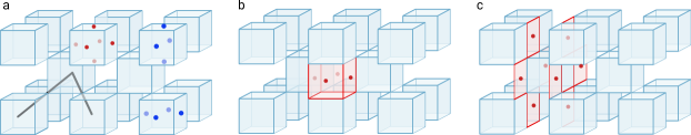
Figure 6: In panel (a), the dimers are shown, which connect cube centers. Panels (a), (b), and (c) list schemes for spin models (red dots indicate locations of spins and blue dots indicate gauage symmetries, in panel [b] red and blue dots coincide) which yield the same thermodynamical properties as the vertex model, but have a $\mathbb{Z}_{2}\times\mathbb{Z}_{2}$ gauge symmetry, a $\mathbb{Z}_{2}$ gauge symmetry, and a planar subsystem symmetry respectively.

In this section, we emphasize that the vertex model dualities are quite general and can be applied to a multitude of other spin models apart from the ones analyzed in the main text. We illustrate this on a lattice of corner-sharing cubes. Place sites in the centers of the cubes, and draw edges between cube centers if they share a corner. The vertex model on the corresponding lattice has $V_{p}=8$. Here, the phase diagram is parameterized by two variables, $u=W(8)/W(4)$ and $v=W(6)/W(4)$ (we will assume $u>v$ for simplicity), and possesses the same symmetry properties as before.

This lattice admits both a Wegner and decorated Wegner duality. In particular, the self dual point $W(n)=\langle\cos^{8-n}\theta\sin^{n}\theta\rangle$ has the weights

$$W(0)=W(8)=\frac{35}{3},\hskip 8.5359ptW(2)=W(6)=\frac{5}{3},\hskip 8.5359ptW(4)=1.$$ (66)

Because of the additional parameter $v$, Wegner’s duality gives a line of self-dual points which solve $u-4v=5$. It turns out that this line of self-dual points can be achieved by selecting the weights

$$W(n,\alpha)=\langle(\cos\theta+\beta\cos 7\theta)^{n}(\sin\theta-\beta\sin 7\theta)^{8-n}\rangle.$$ (67)

We may also access weights off this self dual line through

$$W(n,\alpha)=\langle(\cos\theta+\alpha\cos 3\theta)^{n}(\sin\theta-\alpha\sin 3\theta)^{8-n}\rangle.$$ (68)

In the field theory representation (upon perturbing about the self-dual point where $u=35/3$ and $v=5/3$), the first line of weights will correspond to a sine-Gordon model with a term of the form $\cos(8\theta)$ while the second line of weights corresponds to a sine-Gordon term of the form $\cos(4\theta)$. Since the parameter space is two-dimensional, these are the two operators which control the phase diagram, resulting in the partition functional

$$\int\mathcal{D}\theta(x)\,\exp\left(-\int d^{3}x\,(\nabla\theta)^{2}-\alpha\cos(4\theta)-\beta\cos(8\theta)\right),$$ (69)

which is consistent for the proposed action for $V_{p}=8$ in the main text. In 2+0D, the sine-Gordon term is relevant for $\cos(p\theta)$ where $p^{2}<8\pi$. The $\cos(4\theta)$ term is therefore relevant, and the $\cos(8\theta)$ term is irrelevant, and we expect a gapless line of critical points to exist. However, in 3+0D, both terms are relevant and we expect only a Gaussian fixed point at the self-dual point $u=35/3$ and $v=5/3$. This is conjectural though, and further work is needed to fully characterize the phase diagram of this model.

Next, we construct a spin model equivalent to this vertex model to understand the global and gauge symmetries. On the dual lattice of corner-sharing cubes, the dimers are located at the corners of the cubes, which can be viewed as 12 corner-sharing square plaquettes. There are a multitude of ways in which we can represent dimer variables in terms of spins; three such configurations are shown in Fig. 6. Each spin is identified with the corners of the square it is in the center of. Therefore, for each corner $c$ shared between two cubes, define the dimer variables $d_{c}=\prod_{i\in S}s_{i}^{(c)}$, where $S$ denotes the scheme that is used. For example, in panel [a] there are 6 spins identified with a corner of a cube, so the dimer variable is the product of these 6 spin variables. In panel [b], there are 4 such spins, and in panel [c] there are 2 such spins. As before, $d_{c}=1$ indicates an occupied dimer while $d_{c}=-1$ indicates an empty dimer. For each of the three schemes, we have the relation

$$\prod_{c\in\mbox{\mancube}}d_{c}=\prod_{-\in\mbox{\mancube}}s_{i}^{2}=1,$$ (70)

around each cube, which faithfully reproduces the even dimer constraint. The partition function is $Z_{\text{spin}}=\sum_{\vec{s}}\exp\left(\sum_{\mbox{\mancube}}\mathcal{H}_{\mbox{\mancube}}\right)$, and the Hamiltonian is given by

$$\mathcal{H}_{\mbox{\mancube}}=J_{1}\left(\sum_{c\in\mbox{\mancube}}d_{c}\right)^{2}+J_{2}\left(\sum_{c\in\mbox{\mancube}}d_{c}\right)^{4}.$$ (71)

Note that in this case, a ghost spin cannot be added because the parameter space is much larger. For 4 dimers, $\sum_{c\in\mbox{\mancube}}d_{c}=0$ and the Boltzmann weight $\exp\left(\mathcal{H}_{\mbox{\mancube}}\right)=1$. For 2 and 6 dimers, $\sum_{c\in\mbox{\mancube}}d_{c}=\pm 4$ and for 0 and 8 dimers, $\sum_{c\in\mbox{\mancube}}d_{c}=\pm 8$. Therefore, we solve for the vertex weights in terms of $J_{1}$ and $J_{2}$:

$$W(0) =W(8)=\exp\left(64J_{1}+4096J_{2}\right),$$

$$W(2) =W(6)=\exp\left(16J_{1}+256J_{2}\right),$$ (72)

and $W(4)=1$. At the self dual point, we find

$$e^{J_{1}}=\left(\frac{5}{3}\right)^{5/64}\left(\frac{1}{7}\right)^{1/192}\hskip 14.22636pte^{J_{2}}=\left(\frac{189}{125}\right)^{1/3072}.$$ (73)

In the prior models considered in the main text, we find that there exists both a gauge symmetry and a global symmetry. Here, we find that the spin model possesses different symmetries depending on the scheme. In panel [a], there are two independent gauge symmetries indicated by the two sets of blue sites, which are the generators of a $\mathbb{Z}_{2}\times\mathbb{Z}_{2}$ gauge symmetry. In panel [b], the gauge symmetry is indicated by the red sites, and the model possesses a $\mathbb{Z}_{2}$ gauge symmetry. Interestingly, one may construct a scheme where this gauge symmetry has been “ungauged”, which is shown in panel [c]. Here, the Hamiltonian possesses a planar subsystem symmetry. The nature of these symmetries and the phases of these gauge theories will be the subject of a future work.

Appendix K Details on construction of frustration-free models

We will present the detailed form of the projection operators mentioned in the main text, which allow us to construct the frustration-free Hamiltonians. We first focus on the diamond lattice model. The effective Hamiltonian at sixth order in degenerate perturbation theory treating the XY exchange perturbatively is

$$\mathcal{H}_{\text{eff}}=-c\frac{J_{\perp}^{3}}{J_{z}^{2}}\sum_{\mathord{\raisebox{-1.0pt}{ \leavevmode\hbox to5.35pt{\vbox to4.69pt{\text{[drawing]}}}}}}\left(\prod_{\raisebox{-1.0pt}{\includegraphics[height=6.02777pt]{tetrahedron.png}}\in\mathord{\raisebox{-1.0pt}{ \leavevmode\hbox to5.35pt{\vbox to4.69pt{\text{[drawing]}}}}}}\frac{1+\prod_{i\in\raisebox{-1.0pt}{\includegraphics[height=6.02777pt]{tetrahedron.png}}}Z_{i}}{2}\right)\prod_{j\in\mathord{\raisebox{-1.0pt}{ \leavevmode\hbox to5.35pt{\vbox to4.69pt{\text{[drawing]}}}}}}X_{j},$$ (74)

where the ring exchanges occur on elementary hexagons on the diamond lattice and all configurations are projected onto satisfying the even dimer constraint. Next, it is possible to find a frustration-free point by adding additional interaction terms to this effective Hamiltonian; the ground state can be written as a superposition of classical configurations of a vertex model on the dual lattice. The vertex model has the weights $W_{4}(0)=W_{4}(4)=u$ and $W_{4}(2)=1$; the self-dual/pyrochlore point is $u=3$. Define the projectors

$$\mathcal{P}_{\raisebox{-1.0pt}{\includegraphics[height=6.02777pt]{tetrahedron.png}},i,j}(0) =\sqrt{u}^{-1}\delta(Z_{\raisebox{-1.0pt}{\includegraphics[height=6.02777pt]{tetrahedron.png}}}=0),$$

$$\mathcal{P}_{\raisebox{-1.0pt}{\includegraphics[height=6.02777pt]{tetrahedron.png}},i,j}(2) =\left(\frac{\sqrt{u}-1}{2}\left(1-Z_{i}Z_{j}\right)+1\right)\delta(Z_{\raisebox{-1.0pt}{\includegraphics[height=6.02777pt]{tetrahedron.png}}}=2),$$

$$\mathcal{P}_{\raisebox{-1.0pt}{\includegraphics[height=6.02777pt]{tetrahedron.png}},i,j}(4) =\sqrt{u}^{-1}\delta(Z_{\raisebox{-1.0pt}{\includegraphics[height=6.02777pt]{tetrahedron.png}}}=4),$$ (75)

where the $\delta$-functions are defined as

$$\delta(Z_{\raisebox{-1.0pt}{\includegraphics[height=6.02777pt]{tetrahedron.png}}}=n)=\frac{\prod_{m\neq n}(Z_{\raisebox{-1.0pt}{\includegraphics[height=6.02777pt]{tetrahedron.png}}}-m)}{\prod_{m\neq n}(n-m)}.$$ (76)

These projectors compute the ratio of weights between two vertex configurations $C$ and $C^{\prime}$ which differ by flipping dimers on links $i$ and $j$. We write $\mathcal{P}_{\raisebox{-1.0pt}{\includegraphics[height=6.02777pt]{tetrahedron.png}},i,j}=\sum_{n}\mathcal{P}_{\raisebox{-1.0pt}{\includegraphics[height=6.02777pt]{tetrahedron.png}},i,j}(n)$ and define operators which are products of the above projectors over tetrahedra forming the hexagonal ring exchanges:

$$\mathcal{P}_{\mathord{\raisebox{-1.0pt}{ \leavevmode\hbox to5.35pt{\vbox to4.69pt{\text{[drawing]}}}}}}=\prod_{\raisebox{-1.0pt}{\includegraphics[height=6.02777pt]{tetrahedron.png}},i,j\in\mathord{\raisebox{-1.0pt}{ \leavevmode\hbox to5.35pt{\vbox to4.69pt{\text{[drawing]}}}}}}\mathcal{P}_{\raisebox{-1.0pt}{\includegraphics[height=6.02777pt]{tetrahedron.png}},i,j}.$$ (77)

Then considering

$$\mathcal{H}_{\text{eff}}\longrightarrow\mathcal{H}_{\text{eff}}+c\frac{J_{\perp}^{3}}{J_{z}^{2}}\sum_{\mathord{\raisebox{-1.0pt}{ \leavevmode\hbox to5.35pt{\vbox to4.69pt{\text{[drawing]}}}}}}\left(\prod_{\raisebox{-1.0pt}{\includegraphics[height=6.02777pt]{tetrahedron.png}}\in\mathord{\raisebox{-1.0pt}{ \leavevmode\hbox to5.35pt{\vbox to4.69pt{\text{[drawing]}}}}}}\frac{1+\prod_{i\in\raisebox{-1.0pt}{\includegraphics[height=6.02777pt]{tetrahedron.png}}}Z_{i}}{2}\right)\mathcal{P}_{\mathord{\raisebox{-1.0pt}{ \leavevmode\hbox to5.35pt{\vbox to4.69pt{\text{[drawing]}}}}}},$$ (78)

this new Hamiltonian is frustration free, and the ground state is a superposition of classical vertex configurations $C$ with amplitude $\mathcal{W}(C)$, where $\mathcal{W}(\cdot)$ denotes the Boltzmann weight of a particular vertex model configuration: $\ket{\text{GS}}\propto\sum_{C}\sqrt{\mathcal{W}(C)}\ket{C}$.

For the cubic lattice model, we find that the effective Hamiltonian has its first nontrivial contribution at fourth order in perturbation theory, corresponding to a ring exchange around squares:

$$\mathcal{H}_{\text{eff}}=-c\frac{J_{\perp}^{2}}{J_{z}}\sum_{\square}\left(\prod_{\raisebox{-4.0pt}{\includegraphics[height=9.04166pt]{octahedron.png}}\in\square}\frac{1+\prod_{i\in\raisebox{-4.0pt}{\includegraphics[height=9.04166pt]{octahedron.png}}}Z_{i}}{2}\right)\prod_{j\in\square}X_{j}.$$ (79)

The vertex model has the weights $W_{6}(0)=W_{6}(6)=u$ and $W_{6}(2)=W_{6}(4)=1$; the self-dual/octahedral point is $u=5$. We define similar projectors

$$\mathcal{P}_{\raisebox{-4.0pt}{\includegraphics[height=9.04166pt]{octahedron.png}},i,j}(0) =\sqrt{u}^{-1}\delta(Z_{\raisebox{-4.0pt}{\includegraphics[height=9.04166pt]{octahedron.png}}}=0),$$

$$\mathcal{P}_{\raisebox{-4.0pt}{\includegraphics[height=9.04166pt]{octahedron.png}},i,j}(2) =\left(\frac{\sqrt{u}-1}{4}\left(1-Z_{i}\right)\left(1-Z_{j}\right)+1\right)\delta(Z_{\raisebox{-4.0pt}{\includegraphics[height=9.04166pt]{octahedron.png}}}=2),$$

$$\mathcal{P}_{\raisebox{-4.0pt}{\includegraphics[height=9.04166pt]{octahedron.png}},i,j}(4) =\left(\frac{\sqrt{u}-1}{4}\left(1+Z_{i}\right)\left(1+Z_{j}\right)+1\right)\delta(Z_{\raisebox{-4.0pt}{\includegraphics[height=9.04166pt]{octahedron.png}}}=4),$$

$$\mathcal{P}_{\raisebox{-4.0pt}{\includegraphics[height=9.04166pt]{octahedron.png}},i,j}(6) =\sqrt{u}^{-1}\delta(Z_{\raisebox{-4.0pt}{\includegraphics[height=9.04166pt]{octahedron.png}}}=6),$$ (80)

as well has the product of projectors over octahedra forming a square ring exchange (defining $\mathcal{P}_{\raisebox{-4.0pt}{\includegraphics[height=9.04166pt]{octahedron.png}},i,j}=\sum_{n}\mathcal{P}_{\raisebox{-4.0pt}{\includegraphics[height=9.04166pt]{octahedron.png}},i,j}(n)$ ):

$$\mathcal{P}_{\square}=\prod_{\raisebox{-4.0pt}{\includegraphics[height=9.04166pt]{octahedron.png}}\in\square}\mathcal{P}_{\raisebox{-4.0pt}{\includegraphics[height=9.04166pt]{octahedron.png}}}.$$ (81)

The extended Hamiltonian which is frustration free is

$$\mathcal{H}_{\text{eff}}\longrightarrow\mathcal{H}_{\text{eff}}+c\frac{J_{\perp}^{2}}{J_{z}}\sum_{\square}\left(\prod_{\raisebox{-4.0pt}{\includegraphics[height=9.04166pt]{octahedron.png}}\in\square}\frac{1+\prod_{i\in\raisebox{-4.0pt}{\includegraphics[height=9.04166pt]{octahedron.png}}}Z_{i}}{2}\right)\mathcal{P}_{\square}.$$ (82)

This process can be naturally extended to the case when the coordination number of the lattice is larger than $V_{p}=6$, but we do not attempt to study these models in depth in this paper.

We now focus on the effective Hamiltonian when $u=1$, which we claim to be a commuting projector Hamiltonian. We work with the cubic lattice model, as a similar analysis holds for the diamond lattice model. When $u=1$, one can see that

$$\mathcal{P}_{\raisebox{-4.0pt}{\includegraphics[height=9.04166pt]{octahedron.png}},i,j}=\sum_{n}\mathcal{P}_{\raisebox{-4.0pt}{\includegraphics[height=9.04166pt]{octahedron.png}},i,j}(n)=\frac{1}{2}\left(1-\prod_{i\in\raisebox{-4.0pt}{\includegraphics[height=9.04166pt]{octahedron.png}}}Z_{i}\right).$$ (83)

Therefore, the operator $\mathcal{P}_{\square}$ is given by

$$\mathcal{P}_{\square}=\prod_{\raisebox{-4.0pt}{\includegraphics[height=9.04166pt]{octahedron.png}}\in\square}\frac{1}{2}\left(1-\prod_{i\in\raisebox{-4.0pt}{\includegraphics[height=9.04166pt]{octahedron.png}}}Z_{i}\right).$$ (84)

As the Hamiltonian is projected onto a manifold where $\prod_{i\in\raisebox{-4.0pt}{\includegraphics[height=9.04166pt]{octahedron.png}}}Z_{i}=1$, this quantity is zero. The effective Hamiltonian projected on this manifold at $u=1$ can then be rewritten as

$$\mathcal{H}_{\text{eff}}\propto-\frac{J_{\perp}^{2}}{J_{z}}\sum_{\square}\prod_{i\in\square}X_{i}.$$ (85)

which is exactly solvable, and consists of $m$-particle excitations formed by strings of $Z_{i}$ operators with energy gap $O(J_{\perp}^{2}/J_{z})$. To obtain the $e$ excitations, we must consider an excited state manifold where $\prod_{i\in\raisebox{-4.0pt}{\includegraphics[height=9.04166pt]{octahedron.png}}}Z_{i}=-1$ at some number of octahedra. The quantity $\mathcal{P}_{\square}$ is still a constant when restricted to any of these excited subspaces and the effective Hamiltonian is the same as above with an additive constant. The ground state of the Hamiltonian where $\prod_{i\in\raisebox{-4.0pt}{\includegraphics[height=9.04166pt]{octahedron.png}}}Z_{i}=-1$ at a single octahedron corresponds to a single $e$-particle excitation, which has energy gap $O(J_{z})$. Excited states in this sector correspond to having both $e$ and $m$ excitations, which can be used to form an $\epsilon=e\crossproduct m$ particle. An equivalent way of writing down a Hamiltonian which contains both the $e$ and $m$ particle excitations, akin to the toric code Hamiltonian, is:

$$\mathcal{H}_{\text{cubic}} =-J_{z}\sum_{\raisebox{-4.0pt}{\includegraphics[height=9.04166pt]{octahedron.png}}}\prod_{i\in\raisebox{-4.0pt}{\includegraphics[height=9.04166pt]{octahedron.png}}}Z_{i}-c\frac{J_{\perp}^{2}}{J_{z}}\sum_{\square}\left(\prod_{i\in\square}X_{i}-\prod_{\raisebox{-4.0pt}{\includegraphics[height=9.04166pt]{octahedron.png}}\in\square}\frac{1-Z_{\raisebox{-4.0pt}{\includegraphics[height=9.04166pt]{octahedron.png}}}}{2}\right)$$ (86)

$$\mathcal{H}_{\text{diamond}} =-J_{z}\sum_{\raisebox{-1.0pt}{\includegraphics[height=6.02777pt]{tetrahedron.png}}}\prod_{i\in\raisebox{-1.0pt}{\includegraphics[height=6.02777pt]{tetrahedron.png}}}Z_{i}-c\frac{J_{\perp}^{3}}{J_{z}^{2}}\sum_{\mathord{\raisebox{-1.0pt}{ \leavevmode\hbox to5.35pt{\vbox to4.69pt{\text{[drawing]}}}}}}\left(\prod_{i\in\mathord{\raisebox{-1.0pt}{ \leavevmode\hbox to5.35pt{\vbox to4.69pt{\text{[drawing]}}}}}}X_{i}-\prod_{\raisebox{-1.0pt}{\includegraphics[height=6.02777pt]{tetrahedron.png}}\in\mathord{\raisebox{-1.0pt}{ \leavevmode\hbox to5.35pt{\vbox to4.69pt{\text{[drawing]}}}}}}\frac{1-Z_{\raisebox{-1.0pt}{\includegraphics[height=6.02777pt]{tetrahedron.png}}}}{2}\right).$$ (87)

Appendix L Arrowed quantum vertex model

In this appendix, we derive an alternative formulation of the quantum vertex model where the dimer variables are replaced with arrow variables. Because both the cubic and diamond lattices are bipartite and the vertex weights possess a $\mathbb{Z}_{2}$ symmetry, any configuration of dimers can be mapped onto a configuration of arrows, where a dimer corresponds to an arrow pointing out of the A sublattice and an arrow pointing into the B sublattice. While for bipartite lattices arrow and dimer variables are equivalent, on nonbipartite lattices, these constraints yield vastly different phase diagrams. For a bond vertex model on a non-bipartite lattice, we expect to find the universal self-dual point, while for an arrowed vertex model on the same lattice, we expect the entire RK phase diagram to host a single $\mathbb{Z}_{2}$ topologically ordered phase. This has been established numerically for a couple of examples in Ref. [20] in 2D, and we expect it to hold true in higher dimensions. For this reason, it is worth discussing the construction of arrowed vertex models.

On each edge of the cubic or diamond lattice we place two spins rather than one, and we project onto configurations where the spins are antiparallel to each other, which mimic configurations of arrows. We work under the convention that an arrow points from a down spin to an up spin. We then define the unperturbed Hamiltonians

$$\mathcal{H}_{0,\text{d}} =-J_{z}\sum_{\raisebox{-1.0pt}{\includegraphics[height=6.02777pt]{tetrahedron.png}}}\prod_{i\in\raisebox{-1.0pt}{\includegraphics[height=6.02777pt]{tetrahedron.png}}}Z_{i}+J_{z}\sum_{\langle i,j\rangle}Z_{i}Z_{j}$$ (88)

$$\mathcal{H}_{0,\text{c}} =-J_{z}\sum_{\raisebox{-4.0pt}{\includegraphics[height=9.04166pt]{octahedron.png}}}\prod_{i\in\raisebox{-4.0pt}{\includegraphics[height=9.04166pt]{octahedron.png}}}Z_{i}+J_{z}\sum_{\langle i,j\rangle}Z_{i}Z_{j},$$ (89)

which can easily be generalized to an arbitrary lattice that is nonbipartite. We now include a perturbing Hamiltonian which is an XY exchange on each pair of spins associated to an arrow:

$$\mathcal{H}=\mathcal{H}_{0}+J_{\perp}\sum_{\langle i,j\rangle}\left(X_{i}X_{j}+Y_{i}Y_{j}\right).$$ (90)

To sixth order in perturbation theory assuming that $J_{\perp}\ll J_{z}$, the effective Hamiltonian on the diamond lattice is

$$\mathcal{H}_{\text{eff}}\propto-\frac{J_{\perp}^{6}}{J_{z}^{5}}\sum_{\mathord{\raisebox{-1.0pt}{ \leavevmode\hbox to5.35pt{\vbox to4.69pt{\text{[drawing]}}}}}}\prod_{\langle i,j\rangle\in\mathord{\raisebox{-1.0pt}{ \leavevmode\hbox to5.35pt{\vbox to4.69pt{\text{[drawing]}}}}}}\left(1-Z_{i}Z_{j}\right)X_{i}X_{j},$$ (91)

where the Hilbert space is restricted to configurations satisfying $\prod_{i\in\raisebox{-1.0pt}{\includegraphics[height=6.02777pt]{tetrahedron.png}}}Z_{i}=1$. This Hamiltonian contains processes mimicking arrow reversal around hexagonal plaquettes. For the octahedral model, we find a nontrivial Hamiltonian at fourth order in perturbation theory with a restricted Hilbert space $\prod_{i\in\raisebox{-4.0pt}{\includegraphics[height=9.04166pt]{octahedron.png}}}Z_{i}=1$ and an arrow reversal process around square plaquettes. We next define similar projectors as in Eqns. 77 and  81, and modify the Hamiltonian to

$$\mathcal{H}_{\text{eff},d}\propto-\sum_{\mathord{\raisebox{-1.0pt}{ \leavevmode\hbox to5.35pt{\vbox to4.69pt{\text{[drawing]}}}}}}\prod_{\langle i,j\rangle\in\mathord{\raisebox{-1.0pt}{ \leavevmode\hbox to5.35pt{\vbox to4.69pt{\text{[drawing]}}}}}}X_{i}X_{j}+(1-J)\sum_{\mathord{\raisebox{-1.0pt}{ \leavevmode\hbox to5.35pt{\vbox to4.69pt{\text{[drawing]}}}}}}\mathcal{P}_{\mathord{\raisebox{-1.0pt}{ \leavevmode\hbox to5.35pt{\vbox to4.69pt{\text{[drawing]}}}}}}(u)$$ (92)

$$\mathcal{H}_{\text{eff},c}\propto-\sum_{\square}\prod_{\langle i,j\rangle\in\square}X_{i}X_{j}+(1-J)\sum_{\square}\mathcal{P}_{\square}(u)$$ (93)

where the Hamiltonian is projected onto configurations satisfying the arrow constraint $Z_{i}Z_{j}=-1$ as well as $\prod_{i\in P}Z_{i}=1$ where $P$ is an elementary polyhedron (tetrahedra for the diamond lattice and octahedra for the cubic lattice). As there are two spins per side of the polygon associated with the ring exchange, the notation $\langle i,j\rangle$ refers to both spins.

The phase diagram and transitions are identical to that of the quantum vertex model with dimer variables. In fact, one may verify that the point $u=1$ corresponds to an exactly solvable commuting projector model with toric code topological order where the $m$ excitations have a much smaller gap than the $e$ excitations. The effective Hamiltonian(s) at this point are given by:

$$\mathcal{H}_{d} =-J_{z}\sum_{\raisebox{-1.0pt}{\includegraphics[height=6.02777pt]{tetrahedron.png}}}\prod_{i\in\raisebox{-1.0pt}{\includegraphics[height=6.02777pt]{tetrahedron.png}}}Z_{i}+J_{z}\sum_{\langle i,j\rangle}Z_{i}Z_{j}-c\frac{J_{\perp}^{6}}{J_{z}^{5}}\sum_{\mathord{\raisebox{-1.0pt}{ \leavevmode\hbox to5.35pt{\vbox to4.69pt{\text{[drawing]}}}}}}\left(\prod_{\langle i,j\rangle\in\mathord{\raisebox{-1.0pt}{ \leavevmode\hbox to5.35pt{\vbox to4.69pt{\text{[drawing]}}}}}}X_{i}X_{j}-\prod_{\raisebox{-1.0pt}{\includegraphics[height=6.02777pt]{tetrahedron.png}}\in\mathord{\raisebox{-1.0pt}{ \leavevmode\hbox to5.35pt{\vbox to4.69pt{\text{[drawing]}}}}}}\frac{1-Z_{\raisebox{-1.0pt}{\includegraphics[height=6.02777pt]{tetrahedron.png}}}}{2}\right)$$ (94)

$$\mathcal{H}_{c} =-J_{z}\sum_{\raisebox{-4.0pt}{\includegraphics[height=9.04166pt]{octahedron.png}}}\prod_{i\in\raisebox{-4.0pt}{\includegraphics[height=9.04166pt]{octahedron.png}}}Z_{i}+J_{z}\sum_{\langle i,j\rangle}Z_{i}Z_{j}-c\frac{J_{\perp}^{4}}{J_{z}^{3}}\sum_{\square}\left(\prod_{\langle i,j\rangle\in\square}X_{i}X_{j}-\prod_{\raisebox{-4.0pt}{\includegraphics[height=9.04166pt]{octahedron.png}}\in\square}\frac{1-Z_{\raisebox{-4.0pt}{\includegraphics[height=9.04166pt]{octahedron.png}}}}{2}\right).$$ (95)

References

Wen [2004]X.-G. Wen, Quantum field theory of
many-body systems: from the origin of sound to an origin of light and
electrons (Oxford University Press on Demand, 2004).
Fradkin [2013]E. Fradkin, Field theories of
condensed matter physics (Cambridge University
Press, 2013).