Dynamical friction of black holes in ultralight dark matter

Abstract

In this work we derive simple closed-form expressions for the dynamical friction acting on black holes moving through ultralight (scalar field) dark matter, covering both nonrelativistic and relativistic black hole speeds. Our derivation is based on long known scattering amplitudes in black hole spacetimes, it includes the effect of black hole spin and can be easily extended to vector and tensor light fields. Our results cover and complement recent numerical and previous nonrelativistic treatments of dynamical friction in ultralight dark matter.

I Introduction

The search for new interactions has been a vibrant field for decades, the importance of which is hard to overemphasize. New axionic degrees of freedom, for example, have been predicted to arise in extensions of the Standard Model [1, 2, 3, 4, 5]. In fact, a variety of new scalars could populate the Universe [6]. If such new degrees of freedom are ultralight, they would also be a natural component of dark matter (dm) [7, 8, 9]. These are often referred to as fuzzy dm models, and require ultralight bosonic fields (we refer the reader to Refs. [10, 11, 12, 13, 14, 15, 16, 17, 18]). Such extensions are not restricted to scalars or axions: models of minicharged dark matter predict the existence of new fermions which possess a fractional electric charge or are charged under a hidden $U(1)$ symmetry [19, 20, 21, 22, 23, 24]. These minicharged particles are a viable candidate for cold dm and their properties have been constrained by several cosmological observations and direct-detection experiments [23, 25, 26, 27, 28, 29, 30, 31, 32, 33]. In some other models, dark fermions do not possess (fractional) electric charge but interact among each other only through the exchange of dark photons, the latter being the mediators of a long-range gauge interaction with no coupling to Standard Model particles [34].

With the above as motivation, a substantial amount of work has been dedicated to understand the physics of extended scalar structures. For example, the structure of composite stars containing boson stars in their interior is important to understand how dark matter could pile up and change the composition of neutron stars [35, 36, 37]. For compact configurations, it is important to understand possible gravitational-wave signatures upon coalescence with black holes or other boson stars [38, 39]. When the configuration is dilute however, numerical simulations become extremely challenging or impossible to perform, as the physical effects of interest act on much longer timescales. Of particular importance is dynamical friction (df) and energy loss via scalar emission, which control the motion of objects moving within extended scalar structures [11, 40, 16, 41, 42, 43, 44].

To overcome the different and disparate length scales in any astrophysical scenario, recent numerical simulations modeled the spacetime as a fixed Schwarzschild black hole (bh) geometry, moving at constant velocity through a scalar field environment of infinite extent, and extracted numerically the df [41]. Here, we show that in this setup the df can be obtained analytically. We derive simple expressions, valid both for nonrelativistic and relativistic bh speeds, from scattering amplitudes in bh spacetimes. We focus on stationary regimes and extend the Newtonian expressions in Refs. [11, 40]. Our results complement the recent numerical work of Ref. [41].

In this work we follow the conventions of Ref. [45]; in particular, we adopt the mostly positive metric signature and use geometrized units ($c=G=1$).

II Framework

Ultralight bosons produced through the misalignment mechanism are described by a coherent state [46, 18], for which the relative quantum field fluctuations are suppressed with $1/\sqrt{N}$, where $N$ is the (average) occupancy number of the state [47]. From observations we know that the local dm density in the Solar System’s neighborhood is $\sim 1\,\text{GeV}/\text{cm}^{3}$ [48, 49, 50]. On the other hand, virialized ultralight particles in the Galaxy have a de Broglie wavelength $\lambda_{\text{dB}}\sim\text{kpc}\left(\frac{10^{-22}\text{eV}}{m_{S}}\right)\left(\frac{250\,\text{km/s}}{v}\right)$. So, if these ultralight bosons are all the dm, the typical occupancy number is $N\sim 10^{96}\left(\frac{10^{-22}\text{eV}}{m_{S}}\right)^{4}\left(\frac{250\,\text{km/s}}{v}\right)^{3}$. Thus, this system can be completely described in terms of a classical field [18].

In this work we model the scalar particles through a massive complex scalar field described by the action

$$S=\int d^{4}x\sqrt{-g}\left(\frac{R}{8\pi}-\Phi^{*}_{\;\,,\alpha}\Phi^{\,,\alpha}-\mu^{2}|\Phi|^{2}\right),$$ (1)

where $m_{S}=\hbar\mu$ is the mass of the scalar. Therefore, the scalar field satisfies the Klein-Gordon (kg) equation

$$\Box\Phi=\mu^{2}\Phi,$$ (2)

and the spacetime metric satisfies the Einstein equations

$$G^{\alpha\beta}=8\pi\,T^{\alpha\beta},$$ (3)

where $G^{\alpha\beta}\equiv R^{\alpha\beta}-\frac{1}{2}Rg^{\alpha\beta}$ is the Einstein tensor, and the scalar’s energy-momentum tensor is

$$T^{\alpha\beta}=\nabla^{(\alpha}\Phi^{*}\nabla^{\beta)}\Phi-\frac{1}{2}g^{\alpha\beta}\left(\Phi^{*}_{\;\,;\delta}\Phi^{\,;\delta}+\mu^{2}|\Phi|^{2}\right).$$ (4)

For most situations of interest, the scalar is not very dense and can be studied in a fixed spacetime geometry – the so-called test field approximation. So, let us consider a fixed background metric describing a stationary spinning (Kerr) bh with line element, in Boyer-Lindquist coordinates,

$$ds^{2}= -\frac{\Delta}{\rho_{r}^{2}}(dt-a\sin^{2}\theta\,d\varphi)^{2}+\frac{\rho_{r}^{2}}{\Delta}dr^{2}$$ (5)

$$+\rho_{r}^{2}d\theta^{2}+\frac{\sin^{2}\theta}{\rho_{r}^{2}}\Big{(}adt-(r^{2}+a^{2})d\varphi\Big{)}^{2},$$

where $\rho_{r}^{2}=r^{2}+a^{2}\cos^{2}\theta$ and $\Delta=r^{2}+a^{2}-2Mr$, with $0\leq a\leq M$. Here, $M$ is the bh mass and $J=Ma$ its angular momentum (pointing along $\theta=0$).

III Scalar field scattering off a black hole at rest

A bh moving through an infinite homogeneous scalar field medium is equivalent (by applying a Lorentz boost to the bh frame) to a plane wave scattering off a bh at rest. So, we start by considering the classical problem of a monochromatic plane wave scattering off a Kerr bh in its proper frame. This scattering problem was studied previously in, e.g., Refs. [51, 52, 53, 54, 55, 56, 57, 58].

Let us consider the multipolar decomposition of a monochromatic scalar field of frequency $\omega$,

$$\Phi=\sum_{\ell,m}e^{-i(\omega t-m\varphi)}\text{Ps}_{\ell}^{m}(\cos\theta,\gamma^{2})\mathcal{R}_{\ell}^{m}(r)\,,$$ (6)

where $\text{Ps}_{\ell}^{m}(\cos\theta,\gamma^{2})$ are (oblate) angular spheroidal wave functions of the first kind satisfying the ordinary differential equation (ode) [59]

$$\frac{1}{\sin\theta}\frac{d}{d\theta}\Big{[}\sin\theta\frac{d\text{Ps}}{d\theta}\Big{]}+\Big{[}\lambda_{\ell}^{m}+\gamma^{2}\sin^{2}\theta-\frac{m^{2}}{\sin^{2}\theta}\Big{]}\text{Ps}=0,$$ (7)

with regular conditions at $\theta=\{0,\pi\}$, where

$$\gamma\equiv ik_{\infty}a\,,\qquad k_{\infty}\equiv\sqrt{\omega^{2}-\mu^{2}}\,.$$ (8)

The eigenvalues $\lambda_{l}^{m}$ ($\ell\geq|m|$) are not known in analytic form; asymptotically ($\ell\to\infty$) they are $\lambda_{\ell}^{m}=\ell(\ell+1)+\tfrac{1}{2}(k_{\infty}a)^{2}+\mathcal{O}(\ell^{-2})$ [60]. The above decomposition reduces the kg equation to a radial ode for the functions $\mathcal{R}_{l}^{m}$ [52],

$$\Delta\frac{d}{dr}\left[\Delta\frac{d\mathcal{R}}{dr}\right]+\Big{[}\omega^{2}(r^{2}+a^{2})^{2}-4aMm\omega r$$

$$+(ma)^{2}-(\lambda+\mu^{2}(r^{2}+a^{2}))\Delta\Big{]}\mathcal{R}=0.$$ (9)

Performing the change of variables

$$\frac{dr}{d\chi}=\frac{\Delta}{r^{2}+a^{2}},\quad-\infty<\chi<+\infty,$$ (10)

$$\mathcal{R}=\frac{f}{\sqrt{r^{2}+a^{2}}}\,,$$ (11)

we can rewrite the radial Eq. (9) in the form of a (time-independent) Schrödinger-like equation

$$\frac{d^{2}f}{d\chi^{2}}+k^{2}(\chi)f=0,\\$$ (12a)

with

$$k^{2}[\chi(r)] = \left(\omega-\frac{ma}{r^{2}+a^{2}}\right)^{2}-\frac{\Delta}{(r^{2}+a^{2})^{2}}\bigg{\{}\lambda+\mu^{2}(r^{2}+a^{2})$$ (12b)

$$-2am\omega+\sqrt{r^{2}+a^{2}}\frac{d}{dr}\left[\frac{r\Delta}{(r^{2}+a^{2})^{3/2}}\right]\bigg{\}},$$

The regular solutions to the above equation satisfy the boundary condition [53]

$$f(\chi\to+\infty)\simeq Ie^{-i\left[k_{\infty}r-\eta\log(2k_{\infty}r)\right]}+Re^{i\left[k_{\infty}r-\eta\log(2k_{\infty}r)\right]}\,,$$ (13)

at spatial infinity, and [52]

$$f(\chi\to-\infty)\simeq Te^{-i(\omega-m\Omega_{\text{h}})\chi}\,,$$ (14)

at the bh event horizon $r_{\text{h}}=M+\sqrt{M^{2}-a^{2}}$ (the largest real root of $\Delta$), where $\Omega_{\text{h}}\equiv a/(r_{\text{h}}^{2}+a^{2})$ is the angular velocity of the bh event horizon. All the above amplitudes are also functions of the angular numbers, $R=R_{\ell}^{m},I=I_{\ell}^{m}$ and $T=T_{\ell}^{m}$. We occasionally omit such dependence whenever it is obvious. Above we defined the useful parameter

$$\eta\equiv-M\left(\frac{\omega^{2}+k_{\infty}^{2}}{k_{\infty}}\right).$$ (15)

Its absolute value is the ratio of the characteristic (gravitational) deflection radius $\sim M(\omega^{2}+k_{\infty}^{2})/k_{\infty}^{2}$ (as can be read from Eq. (89)) to the de Broglie wavelength $1/k_{\infty}$. For $\eta^{2}\gg 1$ the scalar field behaves as a beam of classical particles (particle limit), whereas for $\eta^{2}\ll 1$ the wave effects are at their strongest (wave limit).

Note that we must consider only frequencies $\omega>\mu$, which can arrive to spatial infinity and, so, that allow us to define a scattering problem (alternatively, this is enforced by the Lorentz boost from the scalar’s proper frame to the bh frame). The ratios $R/I$ and $T/I$ are fixed by Eqs. (12) (or, equivalently, by (9)) and can always be obtained numerically, e.g., by solving Eq. (9) with boundary condition (14) (where one can put $T=1$, using the linearity of the ode) and comparing the numerical solution with (13). It is easy to show – through the conservation of the Wronskian – that the amplitudes satisfy the relation

$$\left|\frac{T}{I}\right|^{2}=\frac{k_{\infty}}{\omega-m\Omega_{\text{h}}}\left(1-\left|\frac{R}{I}\right|^{2}\right).$$ (16)

A monochromatic plane wave of frequency $\omega$ and wave vector $\bm{k}_{\infty}=k_{\infty}\bm{\xi}$, where $\bm{\xi}=-\cos\beta{\partial}_{z}+\sin\beta{\partial}_{y}$, deformed by a long-range gravitational potential $\eta/r$ can be written in the form [51, 56]

$$e^{-i\left[k_{\infty}r-\eta\log(2k_{\infty}r)\right]\left(\cos\beta\cos\theta+\sin\beta\sin\theta\sin\varphi\right)}\simeq$$

$$\simeq\bigg{(}\frac{e^{-i\left[k_{\infty}r-\eta\log(2k_{\infty}r)\right]}}{k_{\infty}r}\bigg{)}\sum_{\ell,m}(-i)^{m+1}\frac{2\ell+1}{2}\frac{(\ell-m)!}{(\ell+m)!}\text{Ps}_{\ell}^{m}(\cos\beta,\gamma^{2})\text{Ps}_{\ell}^{m}(\cos\theta,\gamma^{2})+\,\textrm{(outgoing wave)}.$$ (17)

So, choosing the incident amplitude

$$I=\frac{2\ell+1}{2}\sqrt{\frac{\hbar n}{\mu}}\frac{(\ell-m)!}{(\ell+m)!}\frac{(-i)^{m+1}\text{Ps}_{\ell}^{m}(\cos\beta,\gamma^{2})}{k_{\infty}},$$ (18)

the solution (6) describes a beam of scalar particles with proper number density $n$ and momentum $\hbar\bm{k}_{\infty}$ scattering off a Kerr bh. Note that we need to include the amplitude $\sqrt{\hbar n/\mu}$, so that the energy density current of the plane wave is $\lim_{r\to\infty}(-T_{t\alpha}\xi^{\alpha})=(nk_{\infty}/\mu)(\hbar\omega)$, i.e., the product of the number density current $nk_{\infty}/\mu$ and the energy of each particle $\hbar\omega$.

III.1 Energy absorption

The energy of the scalar field contained in a spacelike hypersurface $\mathcal{S}_{t^{\prime}}\equiv\{t=t^{\prime}\}$ extending from the horizon to infinity is

$$E(t^{\prime})=\int_{\mathcal{S}_{t^{\prime}}}dV_{3}\,T^{\alpha t}N_{\alpha}\,,$$ (19)

where $N_{\beta}=-\delta_{\beta}^{t}/\sqrt{-g^{tt}}$ is the unit normal covector and $dV_{3}$ is the volume form induced in the hypersurface. Because we are considering the scattering of monochromatic waves $\Phi\propto e^{-i\omega t}$, which results in a time-invariant energy-momentum tensor $T^{\alpha\beta}$, and since the background metric is stationary, one has

$$\frac{dE}{dt^{\prime}}=\int_{\mathcal{S}_{t^{\prime}}}\mathcal{L}_{\partial_{t}}\left(dV_{3}\,T^{\alpha t}N_{\alpha}\right)=0\,,$$ (20)

where $\mathcal{L}_{\partial_{t}}(\cdot)$ is the Lie derivative with respect to $(\partial_{t})^{\alpha}$. Then, by applying the divergence theorem it follows that $\dot{E}_{\text{BH}}$, the energy crossing the event horizon per unit time $t$ (the proper time of a stationary observer at infinity), is equal to the flux through a 2-sphere at spatial infinity

$$\dot{E}_{\text{BH}}=\int_{r\to\infty}d\Omega_{2}\,r^{2}T_{rt},$$ (21)

with the element of area $d\Omega_{2}=\sin\theta\,d\theta d\varphi$.

Plugging the decomposition (6) with the asymptotic solution (13) in the scalar field’s energy-momentum tensor (4) and using the orthogonality relations of the oblate angular spheroidal wave functions [59]

$$\int_{0}^{\pi}d\theta\sin\theta\,\text{Ps}_{\ell}^{m}\text{Ps}_{\ell^{\prime}}^{m}=\frac{2}{2\ell+1}\frac{(\ell+m)!}{(\ell-m)!}\,\delta_{\ell,\ell^{\prime}}$$ (22)

it is straightforward to show that

$$\dot{E}_{\text{BH}}=\omega k_{\infty}\sum_{\ell,m}\frac{4\pi}{2\ell+1}\frac{(\ell+m)!}{(\ell-m)!}\left(|I|^{2}-|R|^{2}\right).$$ (23)

For the case of an incident monochromatic beam described by the amplitude (18), the last expression becomes

$$\dot{E}_{\text{BH}}=\frac{\pi\hbar\omega n}{\mu k_{\infty}}\sum_{\ell,m}(2\ell+1)\frac{(\ell-m)!}{(\ell+m)!}(\text{Ps}_{\ell}^{m})^{2}\bigg{(}1-\bigg{|}\frac{R}{I}\bigg{|}^{2}\bigg{)}.$$ (24)

As a consistency check: note that in a flat spacetime (i.e., $M=0$) the plane wave propagates freely and it is easy to show that $R/I=(-1)^{\ell+1}$, which implies $\dot{E}_{\text{BH}}=0$ as expected (since there is no bh at all); moreover, in the case of a static bh, due to spherical symmetry, one can choose $\beta=0$ without loss of generality, which results in $\text{Ps}_{\ell}^{m}\propto\delta_{m,0}$ and the above expression reduces then to the one found in, e.g., Refs. [53, 61].

To obtain the bh absorption cross section we just need to take the ratio of the energy absorbed by the bh per unit of time $\dot{E}_{\text{BH}}$ to the energy density current of the incident plane wave $(nk_{\infty}/\mu)(\hbar\omega)$,

$$\sigma_{\textrm{abs}}=\frac{\pi}{k_{\infty}^{2}}\sum_{\ell,m}(2\ell+1)\frac{(\ell-m)!}{(\ell+m)!}(\text{Ps}_{\ell}^{m})^{2}\bigg{(}1-\bigg{|}\frac{R}{I}\bigg{|}^{2}\bigg{)}.$$ (25)

III.1.1 Low-frequency limit ($\omega M\ll 1$)

For sufficiently low frequencies $\omega M\ll 1$ one can use matched asymptotic expansions to obtain analytical expressions for the scattering amplitudes (worked out in Appendix A). So, using the reflection amplitude (A.3), at leading order in $\omega M$, the energy absorbed by the bh is

$$\dot{E}_{\text{BH}}\simeq\frac{\hbar\omega^{2}nA_{\text{h}}}{\mu}\frac{e^{-\pi\eta}\pi\eta}{\sinh(\pi\eta)},$$ (26)

and the bh’s absorption cross section is

$$\frac{\sigma_{\textrm{abs}}}{A_{\text{h}}}\simeq\frac{\omega}{k_{\infty}}\frac{e^{-\pi\eta}\pi\eta}{\sinh(\pi\eta)},$$ (27)

where $A_{\text{h}}=4\pi(r_{\text{h}}^{2}+a^{2})$ is the event horizon area. To get this result, we used the fact that at leading order in $\omega M$ only the $l=0$ mode contributes to both $\dot{E}_{\text{BH}}$ and $\sigma_{\textrm{abs}}$, and the spheroidal wave functions become then $\text{Ps}_{0}^{0}(\cos\beta,\gamma^{2})\simeq 1$. We also made use of the property $|\Gamma(1+i\eta)|^{2}=\pi\eta/\sinh(\pi\eta)$. The particle and wave limits of the factor $e^{-\pi\eta}\pi\eta/\sinh(\pi\eta)$ are shown in Table 1.

Particle ($\eta^{2}\gg 1$)	Wave ($\eta^{2}\ll 1$)
$2\pi(-\eta)$	$1$

Table 1: The factor $e^{-\pi\eta}\pi\eta/\sinh(\pi\eta)$ in the particle and wave limits (c.f., Eqs. (26) and (27)).

Note that in the limit $\omega\gg\mu$ we recover the famous result $\sigma_{\textrm{abs}}\simeq A_{\text{h}}$ derived for massless scalar fields in the low-frequency $\omega M\ll 1$ limit [52, 62]. For Schwarzschild bhs ($a=0$) the expressions of this section reduce to the ones obtained decades ago by Unruh [53]. At leading order, the spin dependence of the bh’s absorption cross section is encoded solely in the event horizon area.

We verified that the analytical approximation obtained in Appendix A through matched asymptotic expansions describes perfectly (with an error $\leq 1\%$) the numerical values of $1-|R_{\ell}/I_{\ell}|^{2}$ for $\omega M/(\ell+1)\leq 0.01$. Unfortunately, this approximation rapidly breaks down for larger frequencies; e.g., for $\omega M/(\ell+1)\sim 0.05$ our approximation underestimates in $\sim 15\%$ the true numerical value of $1-|R_{\ell}/I_{\ell}|^{2}$.

III.1.2 High-frequency limit ($\omega M\gg 1$)

For high frequencies $\omega M\gg 1$ one can use the Wentzel-Kramers-Brillouin (wkb) approximation to obtain analytical expressions for the scattering amplitudes (as done in Appendix A). Using the approximation (114) for the reflection amplitude we can directly evaluate Eqs. (24) and (25); this approximation assumes additionally that $\omega\gg\mu$ (which is necessarily true for scalars with $\mu M\leq 1$). For a general incident angle $\beta$ and spin parameter $a$ it is difficult to proceed analytically and one is forced to evaluate these expressions numerically. However, if we restrict to the particular case of small incident angles one can still do a semianalytical treatment; so, we will focus on this particular case.

small incident angles ($\beta\omega M\ll 1$)

From this assumption one has $\text{Ps}_{\ell}^{m}(\cos\beta,\gamma^{2})\simeq\delta_{m0}\text{Ps}_{\ell}^{0}(0,\gamma^{2})$ and that most of the contribution to the summation in $\ell$ comes from large $\ell\gtrsim\omega M$, in which case $\text{Ps}_{\ell}^{0}(0,\gamma^{2})\simeq 1$. Approximating the sum by an integral (an excellent approximation at large $\ell$) we find

$$\dot{E}_{\text{BH}} \simeq \frac{2\pi\hbar n(\omega M)^{2}}{\mu}\int_{0}^{\left(\ell/\omega M\right)_{\text{cr}}}d\Big{(}\frac{\ell}{\omega M}\Big{)}\frac{\ell}{\omega M}$$ (28)

$$= \frac{\pi\hbar n(\omega M)^{2}\left(\ell/\omega M\right)_{\text{cr}}^{2}}{\mu},$$

$$\sigma_{\textrm{abs}} \simeq 2\pi M^{2}\int_{0}^{\left(\ell/\omega M\right)_{\text{cr}}}d\Big{(}\frac{\ell}{\omega M}\Big{)}\frac{\ell}{\omega M}$$ (29)

$$= \pi M^{2}\left(\frac{\ell}{\omega M}\right)_{\text{cr}}^{2}.$$

Here, the critical impact parameter $\left(\ell/\omega M\right)_{\text{cr}}$ is evaluated at $\beta=0$ and can be obtained numerically as a function of the dimensionless spin parameter $\tilde{a}\equiv a/M$ through the procedure described in Appendix B; the result is well fitted by the expression

$$\left(\frac{\ell}{\omega M}\right)_{\text{cr}}\simeq 3\sqrt{3}-0.28\,\tilde{a}^{2}-0.087\,\tilde{a}^{4},$$ (30)

which is accurate to $0.08\%$ in the whole range of $\tilde{a}$. For a nonspinning bh ($\tilde{a}=0$) we recover the well-known result $\sigma_{\textrm{abs}}\simeq 27\pi M^{2}$ [63]. We find that the bh spin leads to a decrease in the energy absorption; in the particular case of small incident angles, the spin can suppress the absorption by up to $13.6\%$.

III.2 Transfer of momentum

In the scattering process there will be a transfer of momentum from the scalar field to the bh, and so the latter will feel a force. Consider the spatial components of the Arnowitt-Deser-Misner (adm) momentum $P^{i}$ computed using a 2-sphere with a sufficiently large radius. These components can be decomposed into the sum of curvature and scalar field contributions $P^{i}=P_{\text{BH}}^{i}+P_{S}^{i}$, where $P_{S}^{i}$ is

$$P_{S}^{i}(t^{\prime})=\int_{S_{t^{\prime}}}dV_{3}T^{\alpha i}N_{\alpha}.$$ (31)

The rate of change of $P^{i}$ is

$$\frac{dP^{i}}{dt^{\prime}}=-\int_{r\to\infty}d\Omega\,r^{2}T^{ri},$$ (32)

and, because we considering a stationary regime, we have

$$\dot{P}_{S}^{i}(t^{\prime})=\int_{\mathcal{S}_{t^{\prime}}}\mathcal{L}_{\partial_{t}}\left(dV_{3}\,T^{\alpha i}N_{\beta}\right)=0.$$ (33)

Thus, the force acting on the bh is

$$F^{i}\equiv\dot{P}^{i}_{\text{BH}}=\dot{P}^{i}=-\int_{r\to\infty}d\Omega_{2}\,r^{2}T^{ri}.$$ (34)

Strictly, in the test field approximation one has $\dot{P}^{i}_{\text{BH}}=0$ (at first order in the scalar field) and $\dot{P}^{i}\neq 0$ (at second order in the scalar field). This is not inconsistent with the last equation, which holds at each order in the scalar field. In other words, would we compute the backreaction of the scalar field on the metric, we would obtain a second order correction to $\dot{P}^{i}_{\text{BH}}$ which must be equal to $\dot{P}^{i}$ (at the same order). For a more thorough discussion, which also covers the case where the steady state is attained dynamically, see Ref. [64].

In asymptotic Cartesian coordinates $(x,y,z)$, defined such that the bh angular momentum is $\bm{J}=J\partial_{z}$ and the direction of incidence is $\bm{\xi}=-\cos\beta{\partial}_{z}+\sin\beta{\partial}_{y}$, we have

$$\lim_{r\to\infty}r^{2}T^{rx} \simeq r^{2}\sin\theta\cos\varphi T_{rr}$$ (35a)

$$= r^{2}\left(\text{P}_{1}^{-1}e^{i\varphi}-\frac{\text{P}_{1}^{1}}{2}e^{-i\varphi}\right)T_{rr},$$

$$\lim_{r\to\infty}r^{2}T^{ry} \simeq r^{2}\sin\theta\sin\varphi T_{rr}$$ (35b)

$$= -i\,r^{2}\left(\text{P}_{1}^{-1}e^{i\varphi}+\frac{\text{P}_{1}^{1}}{2}e^{-i\varphi}\right)T_{rr},$$

$$\lim_{r\to\infty}r^{2}T^{rz} \simeq r^{2}\cos\theta T_{rr}=r^{2}\text{P}_{1}^{0}\,T_{rr},$$

where the $\text{P}_{\ell}^{m}(\cos\theta)$ are associated Legendre polynomials [59]. To evaluate the integrals (34) we will make use of the identity

$$\int d\Omega\,e^{-i(m_{1}+m_{2}-m_{3})\varphi}\text{P}_{\ell_{1}}^{m_{1}}\text{P}_{\ell_{2}}^{m_{2}}\text{P}_{\ell_{3}}^{m_{3}}=\tfrac{4\pi}{2\ell_{3}+1}\sqrt{\tfrac{(\ell_{3}+m_{3})!}{(\ell_{3}-m_{3})!}}$$

$$\times\sqrt{\tfrac{(\ell_{1}+m_{1})!}{(\ell_{1}-m_{1})!}\tfrac{(\ell_{2}+m_{2})!}{(\ell_{2}-m_{2})!}}\left\langle\ell_{1}\,0\,\ell_{2}\,0\middle|\ell_{3}\,0\right\rangle\left\langle\ell_{1}\,m_{1}\,\ell_{2}\,m_{2}\middle|\ell_{3}\,m_{3}\right\rangle,$$

where $\left\langle\ell_{1}\,m_{1}\,\ell_{2}\,m_{2}\middle|\ell_{3}\,m_{3}\right\rangle$ are Clebsch-Gordan coefficients; the last identity is a direct consequence of the Wigner-Eckart theorem. Plugging the decomposition (6) with the asymptotic form (13) in the scalar field’s energy-momentum tensor (4) we find

$$\lim_{r\to\infty}r^{2}T_{rr} = k_{\infty}^{2}\sum_{\ell,m,\ell^{\prime},m^{\prime}}\text{Ps}_{\ell^{\prime}}^{m^{\prime}}\text{Ps}_{\ell}^{m}e^{-i(m^{\prime}-m)\varphi}$$ (37)

$$\times\left(I_{\ell^{\prime}}^{m^{\prime}*}I_{\ell}^{m}+R_{\ell^{\prime}}^{m^{\prime}*}R_{\ell}^{m}\right).$$

III.2.1 Low-frequency limit ($\omega M\ll 1$)

In this limit it is useful to consider the power expansion of the (oblate) angular spheroidal wave functions in $\gamma$ (since $|\gamma|\sim\mathcal{O}(k_{\infty}M)\ll 1$) [65]

$$\text{Ps}_{\ell}^{m}=\text{P}_{\ell}^{m}-\left(\text{a}_{\ell}^{m}\text{P}_{\ell+2}^{m}+\text{b}_{\ell}^{m}\text{P}_{\ell-2}^{m}\right)\gamma^{2}+\mathcal{O}(\gamma^{3}),$$ (38a)

$$\text{a}_{\ell}^{m}=\frac{(\ell-m+1)(\ell-m+2)}{2(2\ell+1)(2\ell+3)^{2}},$$ (38b)

$$\text{b}_{\ell}^{m}=-\frac{(\ell+m-1)(\ell+m)}{2(2\ell-1)^{2}(2\ell+1)}.$$ (38c)

Then, substituting the power expansion (38) in (37) and using Eqs. (35) and (III.2) it is straightforward to show

$$F^{x}=\tfrac{\pi\hbar n}{\mu}\sum_{\ell,m}\bigg{\{}\tfrac{(\ell-m+2)!}{(\ell+m)!}\text{P}_{\ell}^{m}\text{P}_{\ell+1}^{m-1}\Im\left[\Big{(}\tfrac{R_{\ell}^{m}}{I_{\ell}^{m}}\Big{)}^{*}\tfrac{R_{\ell+1}^{m-1}}{I_{\ell+1}^{m-1}}\right]+\tfrac{(\ell-m)!}{(\ell+m)!}\text{P}_{\ell}^{m}\text{P}_{\ell+1}^{m+1}\Im\left[\Big{(}\tfrac{R_{\ell}^{m}}{I_{\ell}^{m}}\Big{)}^{*}\tfrac{R_{\ell+1}^{m+1}}{I_{\ell+1}^{m+1}}\right]\bigg{\}}+\mathcal{O}\left(|\gamma|^{2}\right),$$ (39)

$$F^{y}=-\tfrac{\pi\hbar n}{\mu}\sum_{\ell,m}\bigg{\{}\tfrac{(\ell-m+2)!}{(\ell+m)!}\text{P}_{\ell}^{m}\text{P}_{\ell+1}^{m-1}\Re\left[1+\Big{(}\tfrac{R_{\ell}^{m}}{I_{\ell}^{m}}\Big{)}^{*}\tfrac{R_{\ell+1}^{m-1}}{I_{\ell+1}^{m-1}}\right]-\tfrac{(\ell-m)!}{(\ell+m)!}\text{P}_{\ell}^{m}\text{P}_{\ell+1}^{m+1}\Re\left[1+\Big{(}\tfrac{R_{\ell}^{m}}{I_{\ell}^{m}}\Big{)}^{*}\tfrac{R_{\ell+1}^{m+1}}{I_{\ell+1}^{m+1}}\right]\bigg{\}}+\mathcal{O}\left(|\gamma|^{2}\right),$$ (40)

$$F^{z}=-\tfrac{2\pi\hbar n}{\mu}\sum_{\ell,m}\tfrac{(\ell-m+1)!}{(\ell+m)!}\text{P}_{\ell}^{m}\text{P}_{\ell+1}^{m}\Re\left[1+\Big{(}\tfrac{R_{\ell}^{m}}{I_{\ell}^{m}}\Big{)}^{*}\tfrac{R_{\ell+1}^{m}}{I_{\ell+1}^{m}}\right]+\mathcal{O}\left(|\gamma|^{2}\right),$$ (41)

where the associated Legendre polynomials in the last expressions are evaluated at $\cos\beta$. The symbols $\Re$ and $\Im$ stand, respectively, for the real and imaginary parts of a complex number. Using Eq. (A.3) one can see that at linear order in $\omega M$ the products of reflection amplitudes in the last expressions are independent of $m$. Using the identity

$$\sum_{m}\text{P}_{\ell}^{m}\left[\frac{(\ell-m+2)!}{(\ell+m)!}\text{P}_{\ell+1}^{m-1}+\frac{(\ell-m)!}{(\ell+m)!}\text{P}_{\ell+1}^{m+1}\right]=0,$$ (42)

and (by the scattering amplitude (A.3))

$$\Re\left[1+\bigg{(}\frac{R_{\ell}}{I_{\ell}}\bigg{)}^{*}\frac{R_{\ell+1}}{I_{\ell+1}}\right] \simeq 2\sin^{2}\left(\frac{\alpha_{\ell}}{2}\right)$$ (43)

$$+ \delta_{\ell 0}\frac{\omega k_{\infty}A_{\text{h}}}{2\pi}\frac{e^{-\pi\eta}\pi\eta}{\sinh(\pi\eta)},$$

with the deflection angle

$$\alpha_{\ell}\equiv 2\arg(\ell+1+i\eta)=2\arctan\left(\frac{\eta}{\ell+1}\right),$$ (44)

the force components become (at leading order in $\omega M$)

$$F^{x}\simeq 0,$$ (45)

$$F^{y} \simeq \frac{4\pi\hbar n}{\mu}\sum_{\ell,m}\frac{(\ell-m)!}{(\ell+m)!}\text{P}_{\ell}^{m}\text{P}_{\ell+1}^{m+1}$$ (46)

$$\times\left[\sin^{2}\left(\frac{\alpha_{\ell}}{2}\right)+\delta_{\ell 0}\frac{\omega k_{\infty}A_{\text{h}}}{4\pi}\frac{e^{-\pi\eta}\pi\eta}{\sinh(\pi\eta)}\right],$$

$$F^{z} \simeq -\frac{4\pi\hbar n}{\mu}\sum_{\ell,m}\frac{(\ell-m+1)!}{(\ell+m)!}\text{P}_{\ell}^{m}\text{P}_{\ell+1}^{m}$$ (47)

$$\times\left[\sin^{2}\left(\frac{\alpha_{\ell}}{2}\right)+\delta_{\ell 0}\frac{\omega k_{\infty}A_{\text{h}}}{4\pi}\frac{e^{-\pi\eta}\pi\eta}{\sinh(\pi\eta)}\right].$$

In the Cartesian frame $(\partial_{x^{\prime}},\partial_{y^{\prime}},\partial_{z^{\prime}})$ obtained by rotating $(\partial_{x},\partial_{y},\partial_{z})$ by an angle $\beta$ around $\partial_{x}$ (so that the direction of incidence is $\bm{\xi}=-\partial_{z^{\prime}}$) the components of the force acting on the bh are $F^{x^{\prime}}=F^{x}$, $F^{y^{\prime}}=\cos\beta F^{y}+\sin\beta F^{z}$ and $F^{z^{\prime}}=\cos\beta F^{z}-\sin\beta F^{y}$. Now using the identities

$$\sum_{m}\text{P}_{\ell}^{m}\left[\tfrac{(\ell-m)!}{(\ell+m)!}\text{P}_{\ell+1}^{m+1}\cos\beta+\tfrac{(\ell-m+1)!}{(\ell+m)!}\text{P}_{\ell+1}^{m}\sin\beta\right]=0,$$ (48)

$$\sum_{m}\text{P}_{\ell}^{m}\left[\tfrac{(\ell-m+1)!}{(\ell+m)!}\text{P}_{\ell+1}^{m}\cos\beta-\tfrac{(\ell-m)!}{(\ell+m)!}\text{P}_{\ell+1}^{m+1}\sin\beta\right]=\ell+1,$$ (49)

we obtain

$$F^{x^{\prime}}\simeq F^{y^{\prime}}\simeq 0,$$ (50)

$$F^{z^{\prime}} \simeq -\frac{4\pi\hbar n}{\mu}\left\{\sum_{\ell\geq 1}\ell\sin^{2}\left(\frac{\alpha_{\ell-1}}{2}\right)+\frac{\omega k_{\infty}A_{\text{h}}}{4\pi}\frac{e^{-\pi\eta}\pi\eta}{\sinh(\pi\eta)}\right\}$$

$$= -\frac{4\pi\hbar n}{\mu}\left\{\sum_{\ell\geq 1}\frac{\eta^{2}\ell}{\eta^{2}+\ell^{2}}+\frac{\omega k_{\infty}A_{\text{h}}}{4\pi}\frac{e^{-\pi\eta}\pi\eta}{\sinh(\pi\eta)}\right\}.$$

We see that at leading order in $\omega M$ the force acting on the bh does not depend on the bh spin nor on its angle with respect to the direction of incidence, and it is directed along the direction of incidence $\bm{\xi}$. This can be interpreted as a consequence of the fact that in the limit $\omega M\ll 1$ the force acting on the bh is imparted mostly by scalar field probing the weak (gravitational) field, which is not sensitive to $a$. Actually, the $\ell=0$ mode probes the strong field and is substantially absorbed by the bh, being responsible for the extra term in the above expression, but this contribution is also independent of $a$ because of its spherical symmetry. On the other hand, it is easily seen that the force diverges logarithmically in $\ell$ – which is to be expected due to the long-range $1/r$ nature of the gravitational potential. So, we proceed by introducing a cutoff $\ell_{\text{max}}$, which is associated with the size of the incident beam; the maximum impact parameter is roughly $b_{\text{max}}=\sqrt{\ell_{\text{max}}(\ell_{\text{max}}+1)}/k_{\infty}$ (this cutoff scheme is discussed in more detail in Sec. V). The truncated sum can be written in terms of the digamma function $\Psi$ [59], after which the force becomes

$$F^{z^{\prime}}\simeq-\frac{4\pi\hbar n}{\mu} \left\{\eta^{2}\Re\Big{[}\Psi(1+\ell_{\text{max}}+i\eta)-\Psi(1+i\eta)\Big{]}\right.$$ (52)

$$\left.+\frac{\omega k_{\infty}A_{\text{h}}}{4\pi}\frac{e^{-\pi\eta}\pi\eta}{\sinh(\pi\eta)}\right\}.$$

It is easy to show that in the particle and wave limits the finite sum is excellently approximated by the closed-form expressions in Table 2.

Particle ($\eta^{2}\gg 1$)	Wave ($\eta^{2}\ll 1$)
$(1/2)\log\left(1+k_{\infty}^{2}b_{\text{max}}^{2}/\eta^{2}\right)$	$\log(k_{\infty}b_{\text{max}})+\gamma_{\text{E}}$

Table 2: The term $\Re\big{[}\Psi(1+\ell_{\text{max}}+i\eta)-\Psi(1+i\eta)\big{]}$ in the particle and wave limits (c.f., Eq. (52)); $\gamma_{\textrm{E}}=0.5772\,...$ is Euler’s constant [59].

It is worth noting that, in the eikonal limit $\ell\gg 1$, $\alpha_{\ell}$ is indeed the deflection angle of a particle scattering off a weak gravitational field with impact parameter $b\simeq\ell/k_{\infty}$ and angular momentum $\hbar\ell$. In particular, in the nonrelativistic limit ($\omega\sim\mu$) one finds

$$\alpha_{\ell}\simeq-2\arctan\left(\frac{M\mu^{2}}{b\,k_{\infty}^{2}}\right),$$ (53)

which is exactly the Newtonian deflection angle; and in the ultrarelativistic limit ($\omega\gg\mu$) one gets

$$\alpha_{\ell}\simeq-2\arctan\left(\frac{2M}{b}\right)\simeq-\frac{4M}{b},$$ (54)

which is the deflection angle of light rays obtained by Einstein using his general theory of relativity [67]. If we compute then the force that would act on a source of such weak gravitational field due to a beam of particles coming with momentum $\hbar k_{\infty}$ and impact parameters between $b$ and $b+\delta b$ and being deflected by an angle $\alpha_{\ell}$ we find

$$\frac{\delta F^{z^{\prime}}}{k_{\infty}\delta b}=-\frac{4\pi\hbar n}{\mu}(k_{\infty}b)\sin^{2}\left(\frac{\alpha_{\ell}}{2}\right),$$ (55)

which matches the first term of Eq. (III.2.1) in the eikonal limit; the extra term is due to accretion as explained above.

We verified that the analytic approximation derived in Appendix A and employed here describes quite well (with an error $\leq 5\%$) the numerical values of $\Re\left[1+(R_{\ell}/I_{\ell})^{*}(R_{\ell+1}/I_{\ell+1})\right]$ for $\omega M\leq 0.01$. As for the energy absorption, the analytic approximation breaks down for larger frequencies; e.g., for $\omega M/(l+1)\sim 0.05$ our expression underestimates in $\sim 20\%$ the true numerical value of $\Re\left[1+(R_{\ell}/I_{\ell})^{*}(R_{\ell+1}/I_{\ell+1})\right]$.

III.2.2 High-frequency limit ($\omega M\gg 1$)

To proceed with a semianalytical treatment we focus again on the case of small incident angles.

small incident angles ($\beta\omega M\ll 1$)

In this case we can consider only $m=0$ modes in the scalar’s decomposition (6) (due to the approximate axial symmetry) and we note that most of the contribution to the summation in $\ell$ comes from large $\ell\gtrsim\omega M$, in which case $\text{Ps}_{\ell}^{0}(\cos\theta,\gamma^{2})\simeq\text{P}_{\ell}^{0}(\cos\theta)$. So, using Eqs. (35), (III.2) and (37) it is straightforward to show

$$F^{x}\simeq F^{y}\simeq 0,$$ (56)

$$F^{z}\simeq-\frac{2\pi\hbar n}{\mu}\sum_{\ell}(\ell+1)\Re\left[1+\bigg{(}\frac{R_{\ell}^{0}}{I_{\ell}^{0}}\bigg{)}^{*}\frac{R_{\ell+1}^{0}}{I_{\ell+1}^{0}}\right],$$ (57)

where the reflection amplitudes can be approximated by (114). Here the accretion of scalar field gives an important contribution to the force acting on the bh, which is contained in the terms of (57) with $\ell<\ell_{\text{cr}}$, for which $R/I\simeq 0$. In the high-frequency limit the summation is dominated by the large azimuthal numbers $\ell\gg 1$ and, so, can be approximated by an integral. Thus, the accretion of scalar is responsible for the contribution $-\pi\hbar n\ell_{\text{cr}}^{2}/\mu$ to the force (which, naturally, matches $\dot{E}_{\text{BH}}$ in absolute value, since we are considering the ultrarelativistic regime $\omega\gg\mu$). The remaining contribution from larger $\ell$’s can be obtained by using the eikonal approximation (where $\ell\simeq\omega b$) and rewriting the summation as

$$\sum_{\ell>\ell_{\text{cr}}}(\ell+1)\Re\left[1+\left(\tfrac{R_{\ell}^{0}}{I_{\ell}^{0}}\right)^{*}\tfrac{R_{\ell+1}^{0}}{I_{\ell+1}^{0}}\right]\simeq 2\omega^{2}\int_{\ell_{\text{cr}}/\omega}^{\infty}db\,b\sin^{2}\big{(}\tfrac{\alpha}{2}\big{)},$$ (58)

where

$$\alpha = \pi-2\frac{d}{db}\bigg{[}\chi(r_{\text{tp}})+\int_{r_{\text{tp}}}^{\infty}dr\,\Big{(}\tfrac{r^{2}+a^{2}}{\Delta}\Big{)}\Big{(}1-\tfrac{k}{\omega}\Big{)}\bigg{]}$$ (59)

$$= \pi-2\int_{r_{\text{tp}}}^{\infty}\frac{dr}{\sqrt{\frac{(r^{2}+a^{2})^{2}}{b^{2}}-\Delta}},$$

with $r_{\text{tp}}$ being the larger real number satisfying

$$b=\frac{\omega(r_{\text{tp}}^{2}+a^{2})}{\sqrt{r_{\text{tp}}^{2}+a^{2}-2Mr_{\text{tp}}}}.$$ (60)

Remarkably, the angle $\alpha$ matches exactly the deflection angle of a null particle in a Schwarzschild spacetime when $a=0$ [68, 69, 70]; and, although we did not check it, in the case $a\neq 0$, it is natural to expect $\alpha$ to be the deflection angle of a null particle in a Kerr spacetime for on-axis scattering. It is easy to check that for large impact parameters $b\gg M$ we recover again Einstein’s deflection angle [67]

$$\alpha\simeq-\frac{4M}{b}.$$ (61)

For a beam of scalar particles with maximum impact parameter $b_{\text{max}}>20M$ (remember that the integral in $b$ diverges logarithmically and we need to truncate it) we find

$$\int_{\ell_{\text{cr}}/\omega}^{b_{\text{max}}}db\,b\sin^{2}\left(\frac{\alpha}{2}\right)=4M^{2}\left[\Lambda^{2}+\log\left(\frac{b_{\textrm{max}}}{20M}\right)\right],$$ (62)

where the function $\Lambda$ can be obtained numerically by performing the integration between $\ell_{\text{cr}}/\omega$ and $20M$. This function is well fitted (accurate to 0.1%) by

$$\Lambda\simeq 1.91+0.0565\,\tilde{a}^{2}+0.0165\,\tilde{a}^{4}.$$ (63)

Finally, putting all together (including accretion) we find that the force applied to the bh is

$$F^{z}\simeq-\frac{4\pi\eta^{2}\hbar n}{\mu}\left[\log\left(\frac{b_{\textrm{max}}}{20M}\right)+\frac{\ell_{\text{cr}}^{2}}{16}+\Lambda^{2}\right].$$ (64)

The quantity $\ell_{\text{cr}}^{2}/16+\Lambda^{2}$ has a very mild dependence on $\tilde{a}$, it is strictly increasing and takes values in $[5.31,5.37]$. Here we have $\eta^{2}=(2\omega M)^{2}\gg 1$, which is clearly in the particle limit; this is to be expected, since high-frequency modes are known to be well described by geometrical optics (i.e., geodesics).

IV Black hole moving through a scalar field

Now we know the rate at which energy and linear momentum is imparted to a Kerr bh by a scalar field scattering it off, from the point of view of a distant observer stationary with respect to the bh (”bh frame”). We would like to use this information to find out what are these rates, now from the point of view of a distant observer stationary with respect to the asymptotic scalar field (”scalar field frame”). The latter observer perceives the bh moving with constant velocity $\bm{v}=-\bm{\xi}k_{\infty}/\omega$ with respect to the asymptotic scalar field, which is perceived at rest (by definition). While at rest (and neglecting quantum effects) the bh is a perfect absorber, but when moving it may transfer some of its kinetic energy to the scalar field, with the interesting possibility of, globally, losing energy. The deposition of the bh’s kinetic energy on the scalar field environment is intrinsically connected with the phenomenon of df. Knowing the rate at which energy is accreted and linear momentum is imparted to the moving bh allows us to compute how its relative motion with respect to the scalar field will evolve in time due to df.

The scalar field frame is related to the bh frame through a Lorentz boost with velocity $-\bm{v}$. Noting that the curvature adm four-momentum $P_{\text{BH}}^{\alpha}$ transforms as Lorentz four-vector [71], it is trivial to find the rates in the scalar field frame (primed quantities)

$$\dot{E}^{\prime}_{\text{BH}}=\dot{E}_{\text{BH}}+\bm{v}\cdot\bm{F},$$ (65)

$$\bm{F}^{\prime}=\bm{F}+\dot{E}_{\text{BH}}\bm{v},$$ (66)

where we used $dt^{\prime}=dt/\sqrt{1-v^{2}}$ and $\bm{F}\parallel\bm{v}$. In the general case, the force does not need to point along $\bm{v}$ (e.g., Magnus effect), but as seen in the previous section the force does oppose the velocity in the low-frequency limit or for sufficiently small incident angles – the cases we focused on in this work. The wave effects are controlled by the parameter (15), which, after substituting $\omega=\mu/\sqrt{1-v^{2}}$ and $k_{\infty}=\mu v/\sqrt{1-v^{2}}$, reads

$$\eta=-\frac{\mu M(1+v^{2})}{v\sqrt{1-v^{2}}}.$$ (67)

IV.1 Weak field regime

For bh velocities satisfying $1-v^{2}\gg\mu^{2}M^{2}$ the scalar field is perceived with low frequency ($\omega M\ll 1$) in the bh frame and, so, only probes the weak (Newtonian) gravitational field, as shown in Sec. III. This limit is possible only for light fields $\mu M\ll 1$. On the other hand, for light fields all relevant astrophysical velocities are in this regime; in other words, light fields are not expected to probe the strong gravitational field of bhs, because their de Broglie wavelength is too large.

In the scalar field frame the rate of change of the bh’s energy is

$$\frac{\dot{E}_{\text{BH}}^{\prime}}{\rho}=\frac{A_{\text{h}}}{1-v^{2}}\frac{e^{-\pi\eta}\pi\eta}{\sinh(\pi\eta)}$$

$$-\frac{4\pi\eta^{2}v}{\mu^{2}}\Re\Big{[}\Psi(1+\ell_{\text{max}}+i\eta)-\Psi(1+i\eta)\Big{]},$$ (68)

and the df is

$$\bm{F}^{\prime}=-\frac{4\pi\eta^{2}\rho\bm{v}}{\mu^{2}v}\Re\Big{[}\Psi(1+\ell_{\text{max}}+i\eta)-\Psi(1+i\eta)\Big{]},$$ (69)

where we have defined the scalar’s proper mass density $\rho\equiv nm_{S}$ and the medium size is

$$b_{\text{max}}=\frac{\sqrt{\ell_{\text{max}}(\ell_{\text{max}}+1)(1-v^{2})}}{\mu v}.$$ (70)

We remark that, as discussed in the previous section, the analytic approximations that we are using here can only be trusted (with an error $<5\%$) for $\mu M/\sqrt{1-v^{2}}\leq 0.01$.

In the particle limit $\eta^{2}\gg 1$, which corresponds to nonrelativistic velocities $v\ll\mu M$, the above expressions reduce to

$$\dot{E}^{\prime}_{\text{BH}}=\frac{4\pi M^{2}\rho}{v}\left\{\frac{\mu A_{\text{h}}}{8M}-\log\left(\sqrt{1+\frac{b_{\text{max}}^{2}}{(M/v^{2})^{2}}}\right)\right\},$$ (71)

and

$$\bm{F}^{\prime}=-\frac{4\pi M^{2}\rho\bm{v}}{v^{3}}\log\left(\sqrt{1+\frac{b_{\text{max}}^{2}}{(M/v^{2})^{2}}}\right).$$ (72)

For an extended medium $b_{\text{max}}\gg M/v^{2}$ we recover Chandrasekhar’s result for df in collisionless media [72].

In the wave limit $\eta^{2}\ll 1$, which corresponds to bh velocities $v\gg\mu M$, the rate of change of the bh’s energy becomes

$$\dot{E}_{\text{BH}}^{\prime} = \frac{4\pi M^{2}\rho}{v(1-v^{2})}$$

$$\times\left\{\frac{A_{\text{h}}v}{4\pi M^{2}}-(1+v^{2})^{2}\left[\log\left(\frac{v\mu b_{\text{max}}}{\sqrt{1-v^{2}}}\right)+\gamma_{\text{E}}\right]\right\},$$

and the df

$$\bm{F}^{\prime}=-\frac{4\pi M^{2}\rho(1+v^{2})^{2}\bm{v}}{v^{3}(1-v^{2})}\left[\log\left(\frac{v\mu b_{\text{max}}}{\sqrt{1-v^{2}}}\right)+\gamma_{\text{E}}\right].$$ (74)

We see that the force on the bh is indeed a friction (i.e., it acts to decrease the absolute value of its velocity) in the entire range of $v$. For nonrelativistic velocities this force reduces to

$$\bm{F}^{\prime}=-\frac{4\pi M^{2}\rho\bm{v}}{v^{3}}\left[\log\left(v\mu b_{\text{max}}\right)+\gamma_{\text{E}}\right],$$ (75)

which for an extended medium $b_{\text{max}}\gg 1/v\mu$ coincides with the result derived in [11, 40] and extracted numerically in [41] (up to an additive constant, which is due to a different cutoff scheme, to be discussed in Sec. V).

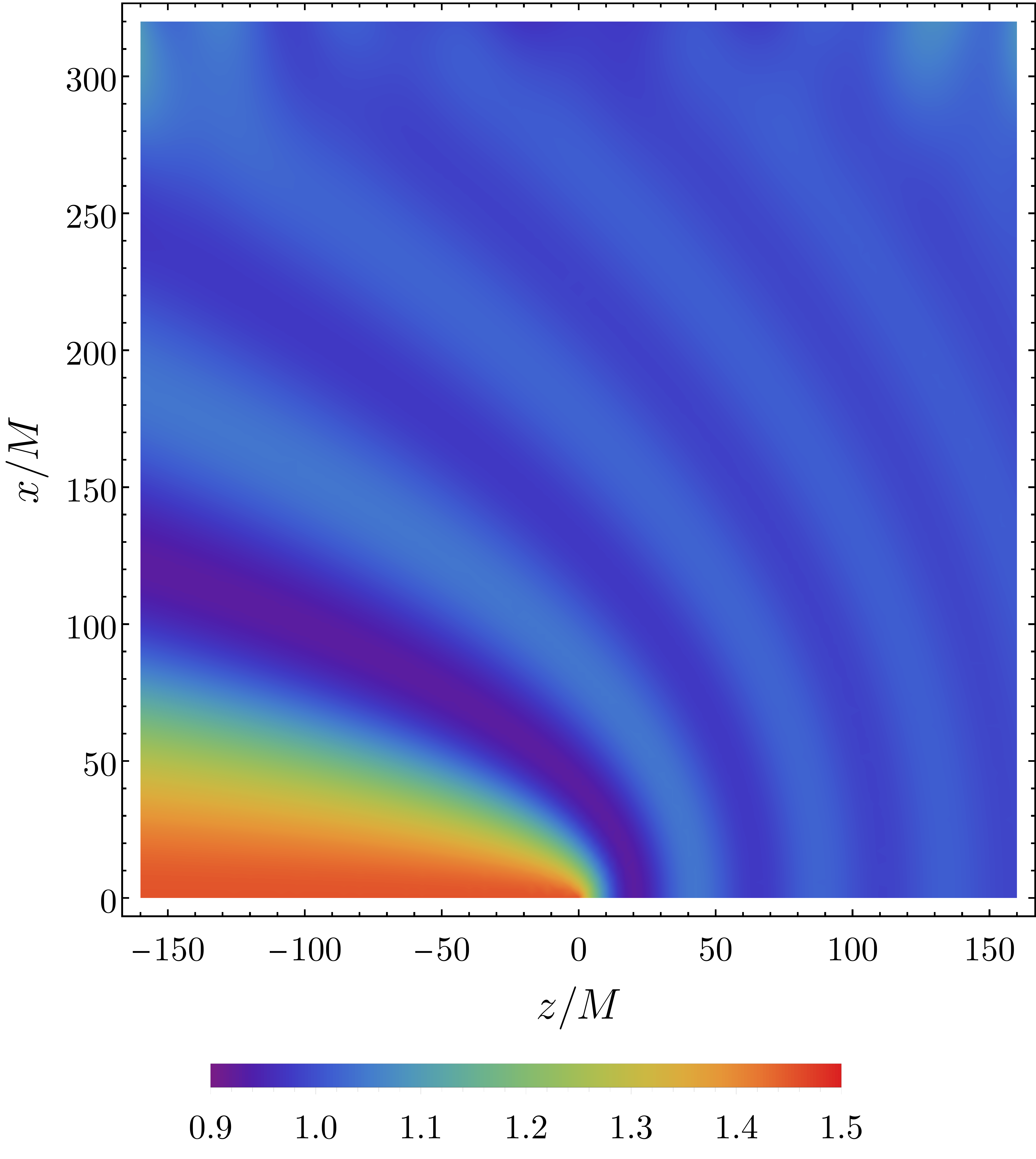
Figure 1: Scalar field energy density $T_{tt}/\rho$ (in the bh frame) in the weak field regime, obtained using the far-region solution (91) with coefficients (98) and (99) (in which we substitute (A.3) and (18)). The bh is at the origin moving from left to right with velocity $v=0.8c$. The scalars have mass $\mu M=0.05$ and $b_{\text{max}}/M\simeq 396$. For these parameters the scalar field is close to the wave limit ($\eta^{2}\simeq 0.016$) as can be clearly seen by the interference fringes with characteristic length $\sim\lambda_{\text{dB}}/2M$.

In Fig. 1 we show the energy density $T_{tt}/\rho$ of the scalar field in the weak field regime, obtained using the far-region solution (91) with coefficients (98) and (99) (in which we substitute (A.3) and (18)). This wake is in the wave limit ($\eta^{2}\ll 1$) and its wave structure (interference fringes) of characteristic length $\sim\lambda_{\text{dB}}/2M=\pi(1+v^{-2})/|\eta|$ is clearly seen. Our figure should be compared with the steady wake attained dynamically in the numerical evolution performed in Ref. [41] (showed in the second row of their Fig. 2 for the same set of parameters); the resemblance between the two images is remarkable. Going away from the wave limit into the particle limit, the fringes disappear and the wake becomes concentrated in a single tail with much greater energy density (as it was seen in [41]).

IV.2 Strong field regime

For velocities $1-v^{2}\ll\mu^{2}M^{2}$ the scalar field is perceived with high-frequency ($\omega M\gg 1$) in the bh frame and, so, it is able to probe the strong gravity region of the bh. Here we restrict to the special case in which the bh motion is along the direction of its spin and we consider light scalars with mass $\mu M\leq 1$. In this case, the condition $1-v^{2}\ll\mu^{2}M^{2}$ is satisfied only at ultrarelativistic speeds $v\sim 1$ and the scalar field behaves as particles ($\eta^{2}\gg 1$).

In the scalar field frame the rate of change of the bh’s energy is

$$\dot{E}_{\text{BH}}^{\prime}=-\frac{16\pi M^{2}\rho}{1-v^{2}}\left[\log\left(\frac{b_{\textrm{max}}}{20M}\right)+\Lambda^{2}\right],$$ (76)

and the df is

$$\bm{F}^{\prime}=-\frac{16\pi M^{2}\rho\bm{v}}{(1-v^{2})v}\left[\log\left(\frac{b_{\textrm{max}}}{20M}\right)+\Lambda^{2}\right],$$ (77)

where we recall that $\Lambda\simeq 1.91+0.0565\tilde{a}^{2}+0.0165\tilde{a}^{4}$ and that these expressions are valid only for $b_{\text{max}}<20M$; for smaller $b_{\text{max}}$ we need to perform a numerical integration.

V Discussion

In this work we derived simple closed-form expressions for the dynamical fiction acting on bhs moving through an ultralight scalar field, covering both nonrelativistic and relativistic speeds, and including the effect of bh spin. We showed that for velocities $1-v^{2}\gg\mu^{2}M^{2}$ the scalar has too large a de Broglie wavelength to probe the strong gravity region of the spacetime (we called it weak field regime). In this case, for low nonrelativistic velocities $v\ll\mu M$ the scalars behave as particles and the force on the bh (in the scalar’s frame) is

$$\bm{F}^{\prime}=-\frac{4\pi M^{2}\rho\bm{v}}{v^{3}}\log\left(\sqrt{1+\frac{b_{\text{max}}^{2}}{(M/v^{2})^{2}}}\right).$$

Still in the weak field regime, the wave effects grow with the bh velocity and are at their greatest for $v\gg\mu M$, in which case

$$\bm{F}^{\prime}=-\frac{4\pi M^{2}\rho(1+v^{2})^{2}\bm{v}}{v^{3}(1-v^{2})}\left[\log\left(\frac{v\mu b_{\text{max}}}{\sqrt{1-v^{2}}}\right)+\gamma_{\text{E}}\right].$$

For light scalar masses $\mu M\leq 1$ and astrophysical bh velocities all systems are expected to be in the weak field regime (even for the possibly relativistic velocities found in bh mergers). We verified that these analytic expressions describe very well the numerical results (obtained using the numerical values for the scattering amplitudes) for $\mu M/\sqrt{1-v^{2}}\leq 0.01$. For the sake of curiosity, for ultrarelativistic bh velocities ($v\sim 1$) satisfying $1-v^{2}\ll\mu^{2}M^{2}$ the scalars are able to probe the strong field region of spacetime (since their de Broglie wavelength becomes much smaller than the event horizon radius) and behave again as particles; here the df is

$$\bm{F}^{\prime}=-\frac{16\pi M^{2}\rho\bm{v}}{(1-v^{2})v}\left[\log\left(\frac{b_{\textrm{max}}}{20M}\right)+\Lambda^{2}\right].$$

Additionally, we derived simple expressions for the rate of change of the bh’s energy, which allows us to do an energy balance between the kinetic energy deposited in the environment and the accreted mass; we also extended these expressions to the case of massless (scalar) radiation, covering the numerical results of Ref. [73].

Due to the $1/r$ falloff of the gravitational potential, the df in an unbounded homogeneous scalar field medium diverges and a cutoff is needed (in practice this is not a problem, because these scalar environments have a finite size, e.g., dm halos). In previous studies (e.g., [11, 40, 64]) an ad hoc cutoff scheme was employed, consisting in neglecting the contribution to df of scalar field from a region outside a ball of radius $r$ centered at the bh. This is clearly not self-consistent, since the wake is computed for a medium of infinite extension. In this work we use a cutoff scheme more similar to the one employed in the original Chandrasekhar’s treatment [72], which consists in considering a maximal impact parameter for the unperturbed medium. This approach is self-consistent since the wake is computed for the truncated medium. But, actually, there is also a subtlety with our cutoff scheme. In the bh frame, our truncated medium is in a superposition of eigenstates of the operator $\hat{L}^{z}$ with maximum eigenvalue $\hbar\ell_{\text{max}}$ and with coefficients such that the expectation value of the asymptotic scalar’s momentum satisfies $\lim_{\ell_{\text{max}}\to\infty}\left<\hat{\bm{p}}_{\infty}\right>=-m_{S}\bm{v}/\sqrt{1-v^{2}}$. So, we note that the interpretation of a bh moving with velocity $\bm{v}$ with respect to the scalars is only correct for $l_{\text{max}}\gg 1$; in particular, in our description there is an inherent velocity dispersion $|\Delta\bm{v}|/v\gtrsim(1-v^{2})/\sqrt{\ell_{\text{max}}(\ell_{\text{max}}+1)}$, by the uncertainty principle. Interestingly, a velocity dispersion of the scalars in a dm halo is actually expected and can be modeled through a random phase distribution, e.g., [40, 18] (in principle, our framework can also be applied to such setup, but we postpone the study of this issue to future work).

For nonrelativistic bh velocities in an extended medium of size $b_{\text{max}}\gg\max\{1/v\mu,M/v^{2}\}$ we recover the Newtonian expressions derived in [11, 40] (up to an additive constant, which comes from the different cutoff scheme used there) and we find that the ratio of the wave to the particle df expressions is

$$\frac{F^{\prime}_{\text{wave}}}{F^{\prime}_{\text{particle}}}=\frac{\log\left(k_{\infty}b_{\text{max}}\right)+\gamma_{E}}{\log\left(k_{\infty}b_{\text{max}}\right)-\log|\eta|},$$ (78)

which is smaller than unity in the wave limit $|\eta|\ll 1$. Remarkably, the above ratio is unchanged for relativistic velocities if for $F_{\text{particle}}^{\prime}$ we use the expression derived in Ref. [74] describing the relativistic df in a collisionless medium. So, we find that the wave effects of light scalars suppress df in an extended medium, both for nonrelativistic and relativistic velocities. This fact, as remarked previously in Ref. [11], can alleviate substantially the timing problem of the five globular clusters in the Fornax dwarf spheroidal [75], and similar issues in faint dwarfs in several nearby galaxy clusters [80, 81].

As inferred in the numerical treatment of Ref. [41], we find that the relativistic corrections to df introduce a factor $(1+v^{2})^{2}/(1-v^{2})$; the same correction was found in [74] for collisionless and in [82] for collisional media. But we argue here that (at least in the weak field regime $1-v^{2}\gg\mu^{2}M^{2}$) this sole factor encodes the entire correction to df and that the extra corrections introduced in [41] are slightly misguided. When boosting from their simulation frame to the bh’s, the authors neglected the contribution of accretion (their Eq. $10$); actually, this contribution is important and it cannot be neglected. Because of that, their results for the df are valid in their simulation coordinates – and not in the bh’s frame. It is easy to show that the force in their simulation frame is equal to the force $\bm{F}^{\prime}$ in the scalar’s frame. As we have shown the accretion of momentum cancels out of $\bm{F}^{\prime}$ (c.f., (66)). So, we argue here that both their ”pressure correction” (depending on a parameter $\kappa$) and Bondi’s momentum accretion are actually describing strong gravity corrections to the df; remember that the weak field analytic expressions that we derived are a good approximation only for $\mu M/\sqrt{1-v^{2}}\leq 0.01$, for larger $\mu M$ strong gravity effects start to kick in. We predict that these corrections will not be needed to fit their results for $\mu M/\sqrt{1-v^{2}}\leq 0.01$. Our suspicions are supported by the fact that using our framework to compute the force $\bm{F}^{\prime}$ with the scattering amplitudes $R/I$ obtained numerically, gives results in remarkable agreement with Ref. [41] (as can be seen in Fig. 2). The main difference between that numerical procedure and the analytic expression (69) are strong gravity corrections (which are suppressed for $\mu M/\sqrt{1-v^{2}}\leq 0.01$). Summarizing, we conclude that in the scalar field frame and in the weak field regime the relativistic corrections to df are encoded solely in the factor $(1+v^{2})^{2}/(1-v^{2})$.

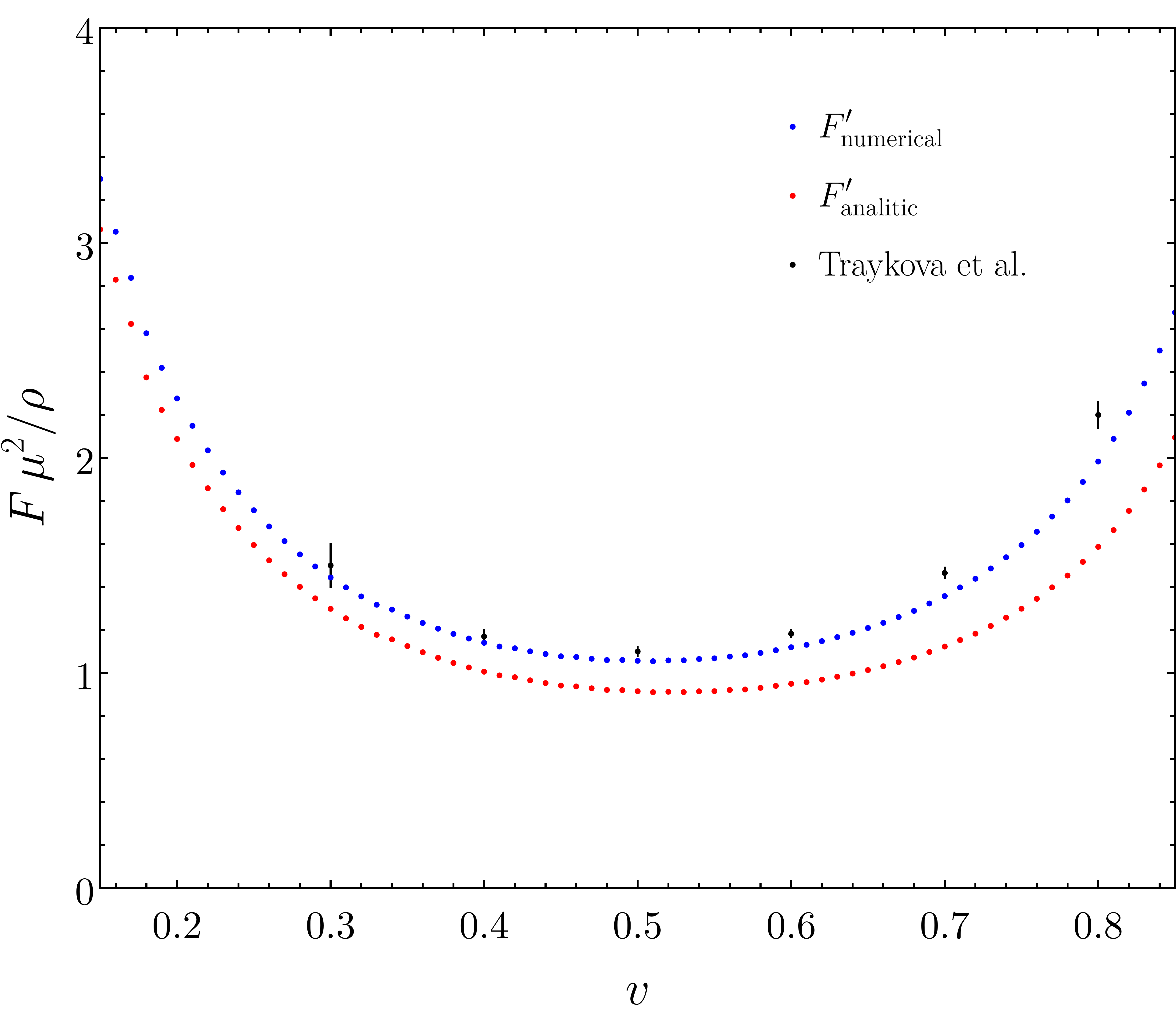
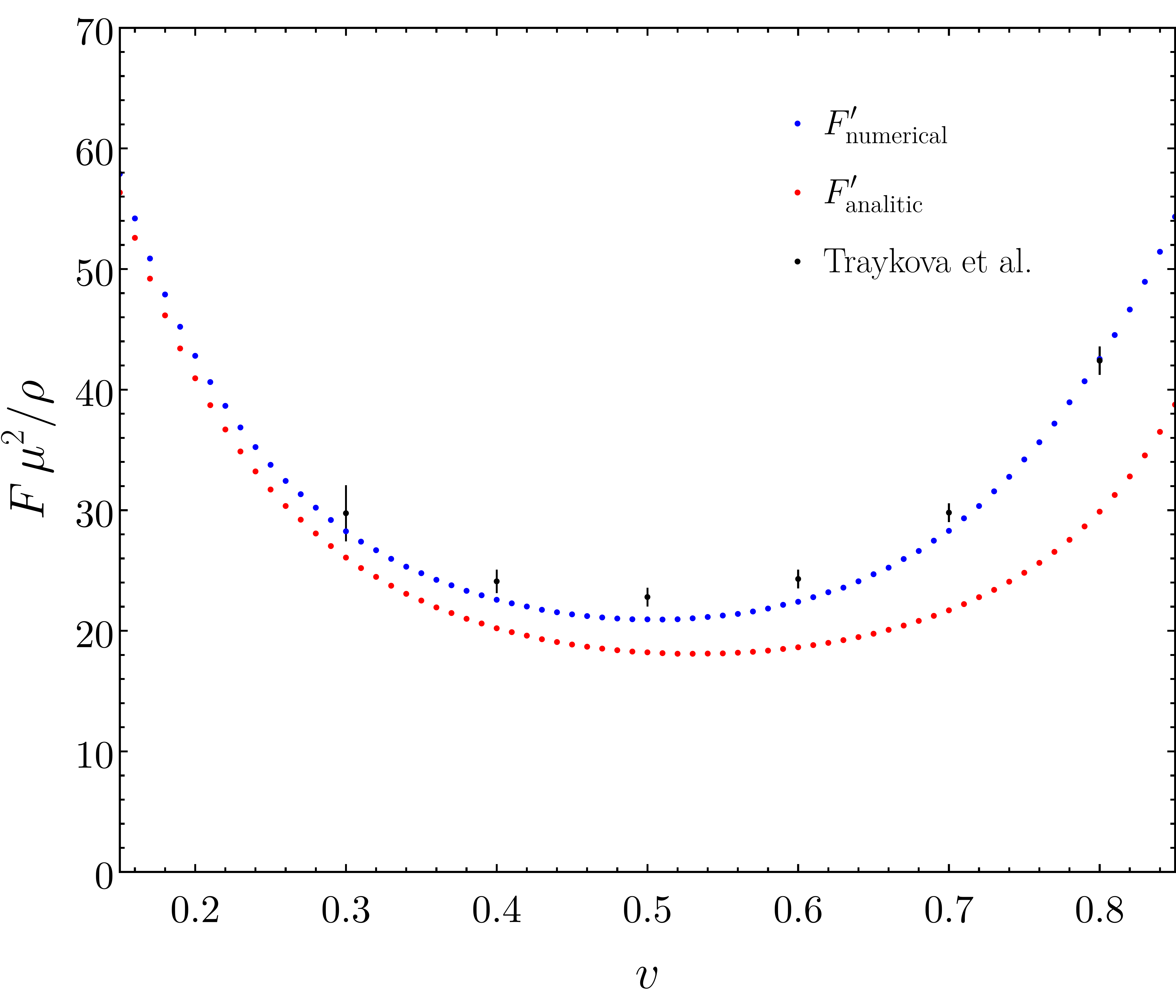
Figure 2: Comparison between the numerical results of Traykova et al. [41] and our framework based on the scattering amplitudes with the $R/I$ obtained numerically ($F^{\prime}_{\text{numerical}}$) and with the analytic approximation of Eq. (69) ($F^{\prime}_{\text{analitic}}$); top panel: $\mu M=0.05$, bottom panel: $\mu M=0.2$. Here, the analytical approximation (69) does not describe very well $F^{\prime}_{\text{numerical}}$ because $\mu M/\sqrt{1-v^{2}}$ is not sufficiently small.

For simplicity, in this work we considered complex scalars, which can arise in simple extensions of the Standard Model [5], but this framework can also be applied to (the more physically motivated) real scalars. In that case, looking at the form of the energy-momentum tensor (4), it is easy to conclude that the scalar’s energy (momentum) density cannot reach a stationary state, but instead it will be left oscillating with frequency $2\omega M=2\mu M/\sqrt{1-v^{2}}$. The df will also oscillate with the same frequency and it is straightforward to show that its average is half of the value of df in the complex case. The same conclusion was also obtained using numerical simulations in [41].

In this work we included also the effect of bh spin in df. In the weak field regime (the most relevant for astrophysical applications) the spin does not affect df in the scalar field frame, and affects accretion only mildly by changing the event horizon area. In the particular case of a bh moving at ultrarelativistic speeds with its spin aligned with the direction of motion, the df is also almost not affected by the bh spin. The strong field regime with a bh spin not aligned with its direction of motion was not studied here; this is the case in which we expect the bh spin to affect the most df. In particular, df will not be in general aligned with the direction of motion and there will be a Magnus effect bending the bh’s trajectory. We postpone the study of this and other interesting phenomena to future work.

Appendix A Scattering amplitudes in the low-frequency limit ($\omega M\ll 1$)

Here we use the method of matched asymptotic expansions to find an approximate analytic expressions for the amplitudes $R/I$ and $T/I$ of massive scalar waves scattering off spinning bhs in the low-frequency limit $\omega M\ll 1$. This is an extension of the treatment in Refs. [52, 83] and [53].

Note that the spheroidal eigenvalues have a power-expansion [59]

$$\lambda_{\ell}^{m}=\ell(\ell+1)+\frac{(k_{\infty}a)^{2}}{2}\bigg{[}1+\frac{(2m-1)(2m+1)}{(2\ell-1)(2\ell+3)}\bigg{]}+\mathcal{O}[(k_{0}a)^{4}]$$ (79)

and, so, in the low-frequency limit $\omega M\ll 1$, the eigenvalues are $\lambda_{\ell}^{m}\simeq\ell(\ell+1)$ at leading order.

A.1 Region I

Let us consider first the region

$$x\equiv\frac{r-r_{\text{h}}}{r_{\text{h}}-r_{\text{c}}}\ll\frac{\ell+1}{\omega(r_{\text{h}}-r_{\text{c}})},$$ (80)

where $r_{\text{c}}=M-\sqrt{M^{2}-a^{2}}$ is the radius of the Cauchy horizon (the smallest real root of $\Delta$). In this region Eq. (9) reduces to [52]

$$x(x+1)\frac{d}{dx}\left[x(x+1)\frac{d\mathcal{R}}{dx}\right]+\big{[}Q^{2}-\ell(\ell+1)x(x+1)\big{]}\mathcal{R}=0,$$ (81)

where

$$Q=\frac{r_{\text{h}}^{2}+a^{2}}{r_{\text{h}}-r_{\text{c}}}(m\Omega_{\text{h}}-\omega).$$ (82)

The general solution of this equation is [59]

$$\mathcal{R} = \left(1+x\right)^{iQ}\bigg{\{}c_{1}x^{-iQ}\,\text{F}(-\ell,\ell+1;1-\bar{Q};-x)$$

$$+c_{2}x^{iQ}\,\text{F}(-\ell+\bar{Q},\ell+1+\bar{Q};1+\bar{Q};-x)\bigg{\}},$$

with $\bar{Q}\equiv 2iQ$ and where $\text{F}(a,b;c;z)$ is the hypergeometric function [59]. The physical boundary conditions (14) at the event horizon ($x\to 0^{+}$) imply that

$$c_{1}=0,$$ (84)

$$c_{2}=\frac{T}{(r_{\text{h}}^{2}+a^{2})^{\frac{1}{2}}}.$$ (85)

Note that the tortoise coordinate $\chi$ in (14) is defined up to an additive constant that we have fixed here through the condition $\chi(r)\simeq\left(\frac{r_{\text{h}}^{2}+a^{2}}{r_{\text{h}}-r_{\text{c}}}\right)\log\left(\frac{r-r_{\text{h}}}{r_{\text{h}}-r_{\text{c}}}\right)$ for $r\sim r_{\text{h}}$.

In the limit $x\gg 1$ one finds that the above solution has the form [83]

$$\mathcal{R}\simeq d_{1}x^{\ell}+\left(\frac{d_{2}}{2\ell+1}\right)x^{-\ell-1},$$ (86)

with

$$d_{1}=T\left[\frac{(2\ell)!}{\ell!\,(1+\bar{Q})_{\ell}\,(r_{\text{h}}^{2}+a^{2})^{\frac{1}{2}}}\right],$$ (87)

$$d_{2}=(-1)^{\ell+1}T\left[\frac{\ell!\,(\bar{Q}-\ell)_{\ell+1}}{2(2\ell)!\,(r_{\text{h}}^{2}+a^{2})^{\frac{1}{2}}}\right],$$ (88)

where $(z)_{n}\equiv z(z+1)\cdots(z+n-1)$ is the Pochhammer symbol.

A.2 Region II

Now we focus on the region $r\gg r_{\text{h}}$ (which implies $x\gg 1$), where Eq. (9) reduces to

$$\left[\frac{d^{2}}{dr^{2}}+k_{\infty}^{2}-\frac{2\eta k_{\infty}}{r}-\frac{\ell(\ell+1)}{r^{2}}\right]\left(\sqrt{\Delta}\,\mathcal{R}\right)=0.$$ (89)

To obtain the last equation we neglected terms of order $(r_{\text{h}}/r)^{3}$, used the low-frequency condition $\omega M\ll 1$, and defined the parameter

$$\eta\equiv-M\left(\frac{\omega^{2}+k_{\infty}^{2}}{k_{\infty}}\right).$$ (90)

This equation admits the solution

$$\mathcal{R}=\frac{c_{3}}{r}\,\text{F}_{\ell}^{C}(\eta,k_{\infty}r)+\frac{c_{4}}{r}\,\text{G}_{\ell}^{C}(\eta,k_{\infty}r),$$ (91)

where $\text{F}_{\ell}^{C}$ and $\text{G}_{\ell}^{C}$ are the Coulomb wave functions [59].

At $k_{\infty}r\ll l$ the solution has the polynomial form [59]

$$\mathcal{R}\simeq c_{3}C_{\ell}(\eta)k_{\infty}^{\ell+1}r^{\ell}+c_{4}\frac{k_{\infty}^{-\ell}r^{-\ell-1}}{(2\ell+1)C_{\ell}(\eta)},$$ (92)

with

$$C_{\ell}=\frac{2^{\ell}e^{-\eta\pi/2}|\Gamma(\ell+1+i\eta)|}{(2\ell+1)!}.$$ (93)

At spatial infinity $k_{\infty}r\to\infty$ it has the asymptotic form

$$\mathcal{R}\simeq\frac{c_{3}}{r}\sin[\theta_{\ell}(\eta,k_{\infty}r)]+\frac{c_{4}}{r}\cos[\theta_{\ell}(\eta,k_{\infty}r)],$$ (94)

where

$$\theta_{\ell}=k_{\infty}r-\eta\log(2k_{\infty}r)-\ell\frac{\pi}{2}+\arg\Gamma(\ell+1+i\eta),$$ (95)

with $\arg(z)$ the principal argument of $z$. The physical boundary conditions (13) imply that

$$I=\left(\frac{c_{4}+ic_{3}}{2}\right)e^{i\left[\ell\pi/2-\arg\Gamma(\ell+1+i\eta)\right]},$$ (96)

$$R=\left(\frac{c_{4}-ic_{3}}{2}\right)e^{-i\left[\ell\pi/2-\arg\Gamma(\ell+1+i\eta)\right]}.$$ (97)

A.3 Matching the two regions

Finally, we just need to match the solutions in the two regions. Matching (92) with (86) at $r_{\text{h}}\ll r\ll 1/k_{\infty}$ gives

$$c_{3}=T\bigg{[}\frac{(2\ell)!\,(M^{2}-a^{2})^{-\frac{\ell}{2}}}{2^{\ell}\,\ell!\,(1+\bar{Q})_{l}\,(r_{\text{h}}^{2}+a^{2})^{1/2}C_{\ell}\,k_{\infty}^{\ell+1}}\bigg{]},$$ (98)

$$c_{4}=(-1)^{\ell+1}\,T\bigg{[}\frac{2^{\ell}\,\ell!\,(\bar{Q}-\ell)_{\ell+1}\,(M^{2}-a^{2})^{\frac{\ell+1}{2}}}{(2\ell)!\,(r_{\text{h}}^{2}+a^{2})^{1/2}C_{\ell}^{-1}k_{\infty}^{-\ell}}\bigg{]}.$$ (99)

So, using Eqs. (96) and (97) we find the following scattering amplitudes:

$$\frac{R}{I}=(-1)^{\ell+1}e^{2i\arg\Gamma(\ell+1+i\eta)}\times$$

$$\Bigg{\{}\frac{[(2\ell)!]^{2}+Q\,(\ell!)^{2}C_{\ell}^{2}\,|(1+2iQ)_{\ell}|^{2}\big{(}2k_{\infty}\sqrt{M^{2}-a^{2}}\,\big{)}^{2\ell+1}}{[(2\ell)!]^{2}-Q\,(\ell!)^{2}C_{\ell}^{2}\,|(1+2iQ)_{\ell}|^{2}\big{(}2k_{\infty}\sqrt{M^{2}-a^{2}}\,\big{)}^{2\ell+1}}\Bigg{\}},$$

$$\frac{T}{I}=(-i)^{\ell+1}e^{i\arg\Gamma(\ell+1+i\eta)}\left(\frac{k_{\infty}}{|\omega-m\Omega_{\text{h}}|}\right)^{\frac{1}{2}}\times$$

$$\Bigg{\{}\frac{2\sqrt{|Q|}\,\ell!\,(2l)!\,C_{\ell}\,(1+2iQ)_{\ell}\,\big{(}2k_{\infty}\sqrt{M^{2}-a^{2}}\,\big{)}^{\ell+\frac{1}{2}}}{[(2\ell)!]^{2}-Q\,(\ell!)^{2}C_{\ell}^{2}\,|(1+2iQ)_{\ell}|^{2}\big{(}2k_{\infty}\sqrt{M^{2}-a^{2}}\,\big{)}^{2\ell+1}}\Bigg{\}}.$$

It is easy to verify that the last expressions satisfy the conservation of the Wronskian (16).

For a static (Schwarzschild) bh we have $a=0$, $r_{\text{h}}=2M$ and $Q=2\omega M\ll 1$, the last expressions simplify to

$$\frac{R}{I} = (-1)^{\ell+1}e^{2i\arg\Gamma(\ell+1+i\eta)}$$

$$\times\Bigg{\{}\frac{[(2\ell)!]^{2}-(\ell!)^{4}C_{\ell}^{2}\,\big{(}2k_{\infty}M\,\big{)}^{2(\ell+1)}(\omega/k_{\infty})}{[(2\ell)!]^{2}+(\ell!)^{4}C_{\ell}^{2}\,\big{(}2k_{\infty}M\,\big{)}^{2(\ell+1)}(\omega/k_{\infty})}\Bigg{\}}$$

$$\simeq (-1)^{\ell+1}e^{2i\arg\Gamma(\ell+1+i\eta)}$$

$$\times\Bigg{\{}1-\left(\frac{2(\ell!)^{4}}{[(2\ell)!]^{2}}\right)\left(\frac{\omega}{k_{\infty}}\right)C_{\ell}^{2}\,\big{(}2k_{\infty}M\,\big{)}^{2(\ell+1)}\Bigg{\}},$$

$$\frac{T}{I} = (-i)^{\ell+1}e^{i\arg\Gamma(\ell+1+i\eta)}$$

$$\times\Bigg{\{}\frac{2\,(\ell!)^{2}\,(2l)!\,C_{\ell}\,\big{(}2k_{\infty}M\,\big{)}^{\ell+1}}{[(2\ell)!]^{2}+(\ell!)^{4}C_{\ell}^{2}\,\big{(}2k_{\infty}M\,\big{)}^{2(\ell+1)}(\omega/k_{\infty})}\Bigg{\}}$$

$$\simeq (-i)^{\ell+1}e^{i\arg\Gamma(\ell+1+i\eta)}\left(\frac{2\,(\ell!)^{2}}{(2\ell)!}\right)C_{\ell}\,\big{(}2k_{\infty}M\,\big{)}^{\ell+1},$$

which agrees with previous calculations [53, 61].

Note that this method does not assume $Q\ll 1$ in the case of a spinning bh, and the expressions for the amplitudes hold for any $Q$ (as long as $\omega M\ll 1$). Since the derivation assumes $\omega M\ll 1$, the expressions (A.3) and (A.3) can be written in the simpler form

$$\frac{R}{I}=(-1)^{\ell+1}e^{2i\arg\Gamma(\ell+1+i\eta)}\times$$

$$\Bigg{\{}1+\left(\frac{2(\ell!)^{2}}{[(2\ell)!]^{2}}\right)Q\,C_{\ell}^{2}\,|(1+2iQ)_{\ell}|^{2}\big{(}2k_{\infty}\sqrt{M^{2}-a^{2}}\,\big{)}^{2\ell+1}\Bigg{\}},$$

$$\frac{T}{I} = (-i)^{\ell+1}e^{i\arg\Gamma(\ell+1+i\eta)}\left(\frac{2\,\ell!}{(2\ell)!}\right)\left(\frac{k_{\infty}}{|\omega-m\Omega_{\text{h}}|}\right)^{\frac{1}{2}}$$ (105)

$$\times \sqrt{|Q|}\,C_{\ell}\,(1+2iQ)_{\ell}\,\big{(}2k_{\infty}\sqrt{M^{2}-a^{2}}\,\big{)}^{\ell+\frac{1}{2}}.$$

To see this one should note that: (i) when $|Q|\to\infty$, $Q|(1+2iQ)_{\ell}|^{2}\sim\mathcal{O}\big{[}1/(M^{2}-a^{2})^{\ell+\frac{1}{2}}\big{]}$; (ii) when $\eta\to-\infty$, $C_{\ell}^{2}\sim\mathcal{O}\big{[}(M\mu^{2}/k_{\infty})^{2\ell+1}\big{]}$, which can be seen more easily through the alternative form of $C_{\ell}$ [59]:

$$C_{\ell}=\frac{2^{\ell}\left\{\big{[}2\pi\eta/\big{(}e^{2\pi\eta}-1\big{)}\big{]}\prod_{j=1}^{\ell}\left(\eta^{2}+j^{2}\right)\right\}^{1/2}}{(2\ell+1)!}.$$ (106)

Appendix B Scattering amplitudes in the high-frequency limit ($\omega M\gg 1$)

In the high-frequency limit we will focus only on the ultrarelativistic regime $\omega\gg\mu$ (which, in particular, is the only possibility for scalars with $\mu M\leq 1$). This limit in frequency was studied for instance in Refs. [63, 84, 56]. For very large azimuthal numbers $\ell\gg\omega M$ using the wkb approximation to solve Eq. (12), with the physical boundary conditions (13) and (14), one finds that [85]

$$\frac{R}{I}=i\exp\Bigg{\{}-2i\omega\bigg{[}\chi(r_{\text{tp}})+\int_{r_{\text{tp}}}^{\infty}dr\,\Big{(}\tfrac{r^{2}+a^{2}}{\Delta}\Big{)}\Big{(}1-\tfrac{k}{\omega}\Big{)}\bigg{]}\Bigg{\}},$$ (107)

where

$$k(r)=\left[\bigg{(}\omega-\frac{ma}{r^{2}+a^{2}}\bigg{)}^{2}-\frac{\Delta}{(r^{2}+a^{2})^{2}}\left(\ell+\tfrac{1}{2}\right)^{2}\right]^{\frac{1}{2}},$$ (108)

and $r_{\text{tp}}$ is the largest classical turning point satisfying $k(r_{\text{tp}})=0$, with the tortoise coordinate fixed by the condition $\chi(r)\simeq r+2M\log(2\omega r)$ for $r\gg r_{\text{h}}$; in particular,

$$\chi(r_{\text{tp}}) = r_{\text{tp}}-\left(\frac{r_{\text{c}}^{2}+a^{2}}{r_{\text{h}}-r_{\text{c}}}\right)\log\left[2\omega(r_{\text{tp}}-r_{\text{c}})\right]$$ (109)

$$+\left(\frac{r_{\text{h}}^{2}+a^{2}}{r_{\text{h}}-r_{\text{c}}}\right)\log\left[2\omega(r_{\text{tp}}-r_{\text{h}})\right].$$

For large azimuthal numbers $\ell\sim\omega M$ it is also possible to use the wkb approximation to compute the absolute value [85]

$$\left|\frac{R}{I}\right|^{2}\simeq\frac{1}{1+e^{2\pi\epsilon}},$$ (110)

where

$$\epsilon=\frac{k_{\min}^{2}}{\sqrt{2\left(\frac{d^{2}}{d\chi^{2}}k^{2}\right)_{\chi_{\min}}}}$$ (111)

with $k_{\min}=k(\chi_{\min})$ and where $\chi_{\min}\left(\frac{\ell}{\omega M},\frac{m}{\ell}\right)$ is the largest (real) root of

$$\left(\frac{d}{d\chi}k^{2}\right)_{\chi_{\min}}=0.$$ (112)

Note that, in the large $\ell$ limit, $\chi_{\min}$ is indeed only a function of the ratios $\ell/\omega M$ and $m/\ell$. Although not easy to show explicitly for a general $a$, in the high-frequency limit $\omega M\gg 1$ we expect $\epsilon$ to be a monotonic rapidly decreasing function of $\ell/\omega M$, crossing zero at a critical $(\ell/\omega M)_{\text{cr}}$ which is a function of $m/\ell$ and $a/M$. This expectation is motivated by what happens for $a=0$, in which case $(\ell/\omega M)_{\text{cr}}=3\sqrt{3}$ and

$$\epsilon=\frac{27(\omega M)^{2}}{2\ell}\left[1-\left(\frac{\ell}{3\sqrt{3}\,\omega M}\right)^{2}\right]$$ (113)

and was confirmed by our numerics. Thus, one concludes that in the high-frequency limit the reflectivity $|R/I|^{2}$ is well-approximated by a very steep function of $\ell/\omega M$ that vanishes for $\ell/\omega M<(\ell/\omega M)_{\text{cr}}$ and is unity for $(\ell/\omega M)>(\ell/\omega M)_{\text{cr}}$. One is, then, led to the (geometrical optics) approximation [66]

$$\frac{R}{I}=\begin{cases}&0,\quad\ell<\ell_{\text{cr}}\\ &ie^{-2i\omega\big{[}\chi(r_{\text{tp}})+\int_{r_{\text{tp}}}^{\infty}dr\,\big{(}\tfrac{r^{2}+a^{2}}{\Delta}\big{)}\big{(}1-\tfrac{k}{\omega}\big{)}\big{]}},\quad\ell\geq\ell_{\text{cr}}\end{cases}.$$ (114)

Note that $(\ell/\omega M)_{\text{cr}}$ is a root of the discriminant of $k^{2}(r)$. This discriminant is a polynomial of degree $8$ in $\omega M/l$ with a double root at zero, two complex roots, two negative and two positive roots (this was established by our numerics for the physical parameters $0\leq a/M\leq 1$ and $-1\leq m/l\leq 1$). We have shown numerically that $(\ell/\omega M)_{\text{cr}}$ is always the largest real $\ell/\omega M$ that is a root of $k^{2}(r)$. This gives us a very efficient way to compute numerically $(\ell/\omega M)_{\text{cr}}$ as function of $m/\ell$ and $a/M$ (shown in Fig. 3). Alternatively, one can use an analogous procedure to compute numerically $(\ell/\omega M)_{\text{cr}}$ as function of $m/\omega M$ and $a/M$ (shown in Fig. 4).

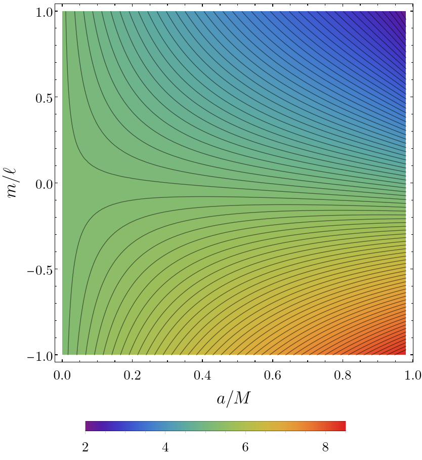
Figure 3: Numerical result of $(\ell/\omega M)_{\text{cr}}$ as function of $a/M$ and $m/\ell$.

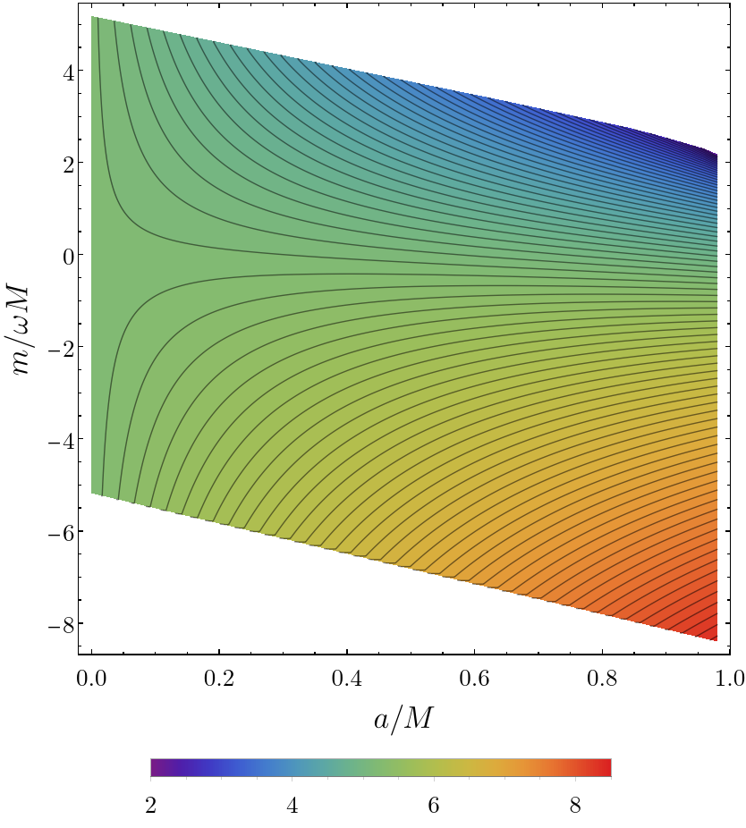
Figure 4: Numerical result of $(\ell/\omega M)_{\text{cr}}$ as function of $a/M$ and $m/\omega M$. In the (unbounded) white region of parameter space there exists no $(\ell/\omega M)_{\text{cr}}$ and expression (107) can be used for any $\ell/\omega M$ (as long as $|m|\leq l$).

Appendix C Black hole moving through a massless scalar field

The problem of obtaining the rate of change of the bh’s energy as it moves through a massless radiation (scalar) field was solved numerically in Ref. [73]. There, it was concluded that, depending on the medium size, there is a critical velocity above which the bh deposits kinetic energy in its environment at a greater rate than it accretes. In this appendix we show that, when moving through a massless scalar field, both the rate of change of the bh’s energy and the df acting on it can be computed analytically.

In the case of a massless scalar field we cannot go to its proper frame. So, we consider here a ”lab frame” with respect to which the bh moves at velocity $\bm{v}$ and the massless scalar has momentum $-\hbar\omega^{\prime}\bm{v}/v$. So, we have $\omega=\sqrt{\frac{1+v}{1-v}}\omega^{\prime}$ and $\bm{k}=-\sqrt{\frac{1+v}{1-v}}\omega^{\prime}\bm{v}/v$ in the bh frame. The factor $n\omega^{\prime}/\mu$ is not well defined here (remember that $n$ is the number density far from the bh in the scalar’s proper frame); this factor must be replaced by the number density in the lab frame $n^{\prime}$ (as can be readily seen by continuity, taking the limit $m_{S}\to 0$).

C.1 Weak field regime

For bh velocities satisfying $1-v\gg\omega^{\prime 2}M^{2}$ the scalar field only probes the weak (Newtonian) gravitational field. In this regime the rate of change of the bh’s energy is

$$\dot{E}^{\prime}_{\text{BH}}=\frac{16\pi M^{2}n^{\prime}\hbar\omega^{\prime}(1+v)v}{1-v}$$

$$\times\left\{\frac{A_{\text{h}}}{16\pi M^{2}}\left(\frac{1}{v}-1\right)-\log\left(\sqrt{\frac{1+v}{1-v}}\omega^{\prime}b_{\text{max}}\right)-\gamma_{\text{EM}}\right\},$$

and the df is

$$(\bm{F})_{\text{lab}} \simeq -\frac{16\pi M^{2}n^{\prime}\hbar\omega^{\prime}(1+v)\bm{v}}{(1-v)v}$$

$$\times\left\{\log\left(\sqrt{\frac{1+v}{1-v}}\omega^{\prime}b_{\text{max}}\right)+\gamma_{\text{EM}}+\frac{A_{\text{h}}(1-v)}{16\pi M^{2}}\right\}.$$

C.2 Strong field regime

For velocities $1-v\ll\omega^{\prime 2}M^{2}$ the scalar field is perceived with high frequency ($\omega M\gg 1$) in the bh frame and, thus, it probes the strong gravity region of the spacetime. We consider the special case in which the bh velocity is along its spin axis. Here the rate of change of the bh’s energy is

$$\dot{E}^{\prime}_{\text{BH}} = \frac{16\pi M^{2}n^{\prime}\hbar\omega^{\prime}(1+v)v}{1-v}$$ (117)

$$\times\left\{\frac{\ell_{\text{cr}}^{2}}{16}\left(\frac{1}{v}-1\right)-\log\left(\frac{b_{\text{max}}}{20M}\right)-\Lambda^{2}\right\},$$

and the force acting on the moving bh is

$$\bm{F}^{\prime} \simeq -\frac{16\pi M^{2}n^{\prime}\hbar\omega^{\prime}(1+v)\bm{v}}{(1-v)v}$$ (118)

$$\times\left\{\log\left(\frac{b_{\text{max}}}{20M}\right)+\Lambda^{2}+\frac{\ell_{\text{cr}}^{2}}{16}(1-v)\right\}.$$

These expressions are valid for media with $b_{\text{max}}\geq 20M$ and the function $\Lambda(\tilde{a})$ is fitted by (63). These analytical expressions describe excellently the numerical results of [73].

References

- Peccei and Quinn [1977] R. D. Peccei and H. R. Quinn, CP Conservation in the Presence of Instantons, Phys. Rev. Lett. 38, 1440 (1977).
- Wilczek [1978] F. Wilczek, Problem of strong and invariance in the presence of instantons, Phys. Rev. Lett. 40, 279 (1978).
- Weinberg [1978] S. Weinberg, A new light boson?, Phys. Rev. Lett. 40, 223 (1978).
- Marsh [2016] D. J. E. Marsh, Axion Cosmology, Phys. Rept. 643, 1 (2016), arXiv:1510.07633 [astro-ph.CO] .
- Freitas et al. [2021] F. F. Freitas, C. A. R. Herdeiro, A. P. Morais, A. Onofre, R. Pasechnik, E. Radu, N. Sanchis-Gual, and R. Santos, Ultralight bosons for strong gravity applications from simple Standard Model extensions, (2021), arXiv:2107.09493 [hep-ph] .
- Arvanitaki et al. [2010] A. Arvanitaki, S. Dimopoulos, S. Dubovsky, N. Kaloper, and J. March-Russell, String Axiverse, Phys. Rev. D81, 123530 (2010), arXiv:0905.4720 [hep-th] .
- Preskill et al. [1983] J. Preskill, M. B. Wise, and F. Wilczek, Cosmology of the Invisible Axion, Phys. Lett. B 120, 127 (1983).
- Abbott and Sikivie [1983] L. F. Abbott and P. Sikivie, A Cosmological Bound on the Invisible Axion, Phys. Lett. B 120, 133 (1983).
- Dine and Fischler [1983] M. Dine and W. Fischler, The Not So Harmless Axion, Phys. Lett. B 120, 137 (1983).
- Robles and Matos [2012] V. H. Robles and T. Matos, Flat Central Density Profile and Constant DM Surface Density in Galaxies from Scalar Field Dark Matter, Mon. Not. Roy. Astron. Soc. 422, 282 (2012), arXiv:1201.3032 [astro-ph.CO] .
- Hui et al. [2017] L. Hui, J. P. Ostriker, S. Tremaine, and E. Witten, Ultralight scalars as cosmological dark matter, Phys. Rev. D95, 043541 (2017), arXiv:1610.08297 [astro-ph.CO] .
- Bar et al. [2019] N. Bar, K. Blum, J. Eby, and R. Sato, Ultralight dark matter in disk galaxies, Phys. Rev. D99, 103020 (2019), arXiv:1903.03402 [astro-ph.CO] .
- Bar et al. [2018] N. Bar, D. Blas, K. Blum, and S. Sibiryakov, Galactic rotation curves versus ultralight dark matter: Implications of the soliton-host halo relation, Phys. Rev. D98, 083027 (2018), arXiv:1805.00122 [astro-ph.CO] .
- Desjacques and Nusser [2019] V. Desjacques and A. Nusser, Axion core–halo mass and the black hole–halo mass relation: constraints on a few parsec scales, Mon. Not. Roy. Astron. Soc. 488, 4497 (2019), arXiv:1905.03450 [astro-ph.CO] .
- Davoudiasl and Denton [2019] H. Davoudiasl and P. B. Denton, Ultralight Boson Dark Matter and Event Horizon Telescope Observations of M87*, Phys. Rev. Lett. 123, 021102 (2019), arXiv:1904.09242 [astro-ph.CO] .
- Annulli et al. [2020] L. Annulli, V. Cardoso, and R. Vicente, Response of ultralight dark matter to supermassive black holes and binaries, Phys. Rev. D102, 063022 (2020), arXiv:2009.00012 [gr-qc] .
- Ferreira [2021] E. G. M. Ferreira, Ultra-light dark matter, Astron. Astrophys. Rev. 29, 7 (2021), arXiv:2005.03254 [astro-ph.CO] .
- Hui [2021] L. Hui, Wave Dark Matter 10.1146/annurev-astro-120920-010024 (2021), arXiv:2101.11735 [astro-ph.CO] .
- De Rujula et al. [1990] A. De Rujula, S. L. Glashow, and U. Sarid, Charged dark matter, Nucl. Phys. B333, 173 (1990).
- Perl and Lee [1997] M. L. Perl and E. R. Lee, The search for elementary particles with fractional electric charge and the philosophy of speculative experiments, Am. J. Phys. 65, 698 (1997).
- Holdom [1986] B. Holdom, Two U(1)’s and Epsilon Charge Shifts, Phys. Lett. B166, 196 (1986).
- Sigurdson et al. [2004] K. Sigurdson, M. Doran, A. Kurylov, R. R. Caldwell, and M. Kamionkowski, Dark-matter electric and magnetic dipole moments, Phys. Rev. D70, 083501 (2004), [Erratum: Phys. Rev.D73,089903(E) (2006)], arXiv:astro-ph/0406355 [astro-ph] .
- Davidson et al. [2000] S. Davidson, S. Hannestad, and G. Raffelt, Updated bounds on millicharged particles, JHEP 05, 003, arXiv:hep-ph/0001179 [hep-ph] .
- McDermott et al. [2011] S. D. McDermott, H.-B. Yu, and K. M. Zurek, Turning off the Lights: How Dark is Dark Matter?, Phys. Rev. D83, 063509 (2011), arXiv:1011.2907 [hep-ph] .
- Dubovsky et al. [2004] S. L. Dubovsky, D. S. Gorbunov, and G. I. Rubtsov, Narrowing the window for millicharged particles by CMB anisotropy, JETP Lett. 79, 1 (2004), [Pisma Zh. Eksp. Teor. Fiz.79,3(2004)], arXiv:hep-ph/0311189 [hep-ph] .
- Gies et al. [2006a] H. Gies, J. Jaeckel, and A. Ringwald, Polarized Light Propagating in a Magnetic Field as a Probe of Millicharged Fermions, Phys. Rev. Lett. 97, 140402 (2006a), arXiv:hep-ph/0607118 [hep-ph] .
- Gies et al. [2006b] H. Gies, J. Jaeckel, and A. Ringwald, Accelerator Cavities as a Probe of Millicharged Particles, Europhys. Lett. 76, 794 (2006b), arXiv:hep-ph/0608238 [hep-ph] .
- Perl et al. [2009] M. L. Perl, E. R. Lee, and D. Loomba, Searches for fractionally charged particles, Ann. Rev. Nucl. Part. Sci. 59, 47 (2009).
- Burrage et al. [2009] C. Burrage, J. Jaeckel, J. Redondo, and A. Ringwald, Late time CMB anisotropies constrain mini-charged particles, JCAP 0911, 002, arXiv:0909.0649 [astro-ph.CO] .
- Ahlers [2009] M. Ahlers, The Hubble diagram as a probe of mini-charged particles, Phys. Rev. D80, 023513 (2009), arXiv:0904.0998 [hep-ph] .
- Haas et al. [2015] A. Haas, C. S. Hill, E. Izaguirre, and I. Yavin, Looking for milli-charged particles with a new experiment at the LHC, Phys. Lett. B746, 117 (2015), arXiv:1410.6816 [hep-ph] .
- Kadota et al. [2016] K. Kadota, T. Sekiguchi, and H. Tashiro, A new constraint on millicharged dark matter from galaxy clusters, (2016), arXiv:1602.04009 [astro-ph.CO] .
- Gondolo and Kadota [2016] P. Gondolo and K. Kadota, Kinetic Decoupling of Light Magnetic Dipole Dark Matter, (2016), arXiv:1603.05783 [hep-ph] .
- Ackerman et al. [2009] L. Ackerman, M. R. Buckley, S. M. Carroll, and M. Kamionkowski, Dark Matter and Dark Radiation, Proceedings, 7th International Heidelberg Conference on Dark Matter in Astro and Particle Physics (DARK 2009), Phys. Rev. D79, 023519 (2009), [,277(2008)], arXiv:0810.5126 [hep-ph] .
- Brito et al. [2015] R. Brito, V. Cardoso, and H. Okawa, Accretion of dark matter by stars, Phys. Rev. Lett. 115, 111301 (2015), arXiv:1508.04773 [gr-qc] .
- Brito et al. [2016] R. Brito, V. Cardoso, C. F. B. Macedo, H. Okawa, and C. Palenzuela, Interaction between bosonic dark matter and stars, Phys. Rev. D93, 044045 (2016), arXiv:1512.00466 [astro-ph.SR] .
- Di Giovanni et al. [2021] F. Di Giovanni, N. Sanchis-Gual, P. Cerdá-Durán, and J. A. Font, Can fermion-boson stars reconcile multi-messenger observations of compact stars?, (2021), arXiv:2110.11997 [gr-qc] .
- Cardoso et al. [2016] V. Cardoso, S. Hopper, C. F. B. Macedo, C. Palenzuela, and P. Pani, Gravitational-wave signatures of exotic compact objects and of quantum corrections at the horizon scale, Phys. Rev. D94, 084031 (2016), arXiv:1608.08637 [gr-qc] .
- Palenzuela et al. [2017] C. Palenzuela, P. Pani, M. Bezares, V. Cardoso, L. Lehner, and S. Liebling, Gravitational Wave Signatures of Highly Compact Boson Star Binaries, Phys. Rev. D96, 104058 (2017), arXiv:1710.09432 [gr-qc] .
- Lancaster et al. [2020] L. Lancaster, C. Giovanetti, P. Mocz, Y. Kahn, M. Lisanti, and D. N. Spergel, Dynamical Friction in a Fuzzy Dark Matter Universe, JCAP 01, 001, arXiv:1909.06381 [astro-ph.CO] .
- Traykova et al. [2021] D. Traykova, K. Clough, T. Helfer, P. G. Ferreira, E. Berti, and L. Hui, Dynamical friction from scalar dark matter in the relativistic regime, (2021), arXiv:2106.08280 [gr-qc] .
- Chowdhury et al. [2021] D. D. Chowdhury, F. C. van den Bosch, V. H. Robles, P. van Dokkum, H.-Y. Schive, T. Chiueh, and T. Broadhurst, On the Random Motion of Nuclear Objects in a Fuzzy Dark Matter Halo, Astrophys. J. 916, 27 (2021), arXiv:2105.05268 [astro-ph.GA] .
- Wang and Easther [2021] Y. Wang and R. Easther, Dynamical Friction From Ultralight Dark Matter, (2021), arXiv:2110.03428 [gr-qc] .
- Baumann et al. [2021] D. Baumann, G. Bertone, J. Stout, and G. M. Tomaselli, Ionization of Gravitational Atoms, (2021), arXiv:2112.14777 [gr-qc] .
- Wald [1984] R. M. Wald, General Relativity (Chicago Univ. Pr., Chicago, USA, 1984).
- Davidson [2015] S. Davidson, Axions: Bose Einstein Condensate or Classical Field?, Astropart. Phys. 65, 101 (2015), arXiv:1405.1139 [hep-ph] .
- Glauber [1963] R. J. Glauber, Coherent and incoherent states of the radiation field, Phys. Rev. 131, 2766 (1963).
- Bovy and Tremaine [2012] J. Bovy and S. Tremaine, On the local dark matter density, Astrophys. J. 756, 89 (2012), arXiv:1205.4033 [astro-ph.GA] .
- Sivertsson et al. [2018] S. Sivertsson, H. Silverwood, J. I. Read, G. Bertone, and P. Steger, The localdark matter density from SDSS-SEGUE G-dwarfs, Mon. Not. Roy. Astron. Soc. 478, 1677 (2018), arXiv:1708.07836 [astro-ph.GA] .
- McKee et al. [2015] C. F. McKee, A. Parravano, and D. J. Hollenbach, Stars, gas, and dark matter in the solar neighborhood, Astrophys. J. 814, 13 (2015).
- Matzner [1968] R. A. Matzner, Scattering of massless scalar waves by a schwarzschild “singularity”, J. Math. Phys. 9, 163 (1968).
- Starobinski [1973] A. Starobinski, Amplification of waves during reflection from a rotating black hole, Zh. Eksp. Teor. Fiz. 64, 48 (1973), (Sov. Phys. - JETP, 37, 28, 1973).
- Unruh [1976] W. G. Unruh, Absorption Cross-Section of Small Black Holes, Phys. Rev. D14, 3251 (1976).
- Sanchez [1978] N. G. Sanchez, Absorption and Emission Spectra of a Schwarzschild Black Hole, Phys. Rev. D18, 1030 (1978).
- Chandrasekhar [1983] S. Chandrasekhar, The Mathematical Theory of Black Holes (Oxford University Press, New York, 1983).
- Glampedakis and Andersson [2001] K. Glampedakis and N. Andersson, Scattering of scalar waves by rotating black holes, Class. Quant. Grav. 18, 1939 (2001), arXiv:gr-qc/0102100 [gr-qc] .
- Macedo et al. [2013] C. F. B. Macedo, L. C. S. Leite, E. S. Oliveira, S. R. Dolan, and L. C. B. Crispino, Absorption of planar massless scalar waves by Kerr black holes, Phys. Rev. D88, 064033 (2013), arXiv:1308.0018 [gr-qc] .
- Leite et al. [2016] L. C. S. Leite, L. C. B. Crispino, E. S. De Oliveira, C. F. B. Macedo, and S. R. Dolan, Absorption of massless scalar field by rotating black holes, Proceedings, 3rd Amazonian Symposium on Physics: Belem, Brazil, September 28-October 2, 2015, Int. J. Mod. Phys. D25, 1641024 (2016).
- [59] NIST Digital Library of Mathematical Functions, http://dlmf.nist.gov/, Release 1.1.2 of 2021-06-15, F. W. J. Olver, A. B. Olde Daalhuis, D. W. Lozier, B. I. Schneider, R. F. Boisvert, C. W. Clark, B. R. Miller, B. V. Saunders, H. S. Cohl, and M. A. McClain, eds.
- Berti et al. [2006] E. Berti, V. Cardoso, and M. Casals, Eigenvalues and eigenfunctions of spin-weighted spheroidal harmonics in four and higher dimensions, Phys. Rev. D73, 024013 (2006), [Erratum: Phys. Rev.D73,109902(E) (2006)], arXiv:gr-qc/0511111 [gr-qc] .
- Vicente [2021] R. Vicente, The Gravity of Classical Fields: And Its Effect on the Dynamics of Gravitational Systems, PhD thesis (2021), arXiv:2110.07620 [gr-qc] .
- Das et al. [1997] S. R. Das, G. W. Gibbons, and S. D. Mathur, Universality of low-energy absorption cross-sections for black holes, Phys. Rev. Lett. 78, 417 (1997), arXiv:hep-th/9609052 [hep-th] .
- Sanchez [1976] N. G. Sanchez, Scattering of scalar waves from a schwarzschild black hole, J. Math. Phys. 17, 688 (1976).
- Clough [2021] K. Clough, Continuity equations for general matter: applications in numerical relativity, Class. Quant. Grav. 38, 167001 (2021), arXiv:2104.13420 [gr-qc] .
- [65] E. W. Weisstein, Spheroidal wave function. From MathWorld—A Wolfram Web Resource.
- Ford and Wheeler [1959] K. W. Ford and J. A. Wheeler, Semiclassical description of scattering, Ann. Phys. 7, 259 (1959).
- Einstein [1936] A. Einstein, Lens-like action of a star by the deviation of light in the gravitational field, Science 84 2188, 506 (1936).
- Darwin [1959] C. G. Darwin, The gravity field of a particle, Proc. R. Soc. London, Ser. A 249, 180 (1959), https://royalsocietypublishing.org/doi/pdf/10.1098/rspa.1959.0015 .
- Misner et al. [1973] C. W. Misner, K. S. Thorne, and J. A. Wheeler, Gravitation (W. H. Freeman, San Francisco, 1973).
- Bisnovatyi-Kogan and Tsupko [2008] G. S. Bisnovatyi-Kogan and O. Y. Tsupko, Strong Gravitational Lensing by Schwarzschild Black Holes, Astrophysics 51, 99 (2008), arXiv:0803.2468 [astro-ph] .
- Arnowitt et al. [2008] R. L. Arnowitt, S. Deser, and C. W. Misner, The Dynamics of general relativity, Gen. Rel. Grav. 40, 1997 (2008), arXiv:gr-qc/0405109 .
- Chandrasekhar [1943] S. Chandrasekhar, Dynamical Friction. I. General Considerations: the Coefficient of Dynamical Friction., Astrophys. J. 97, 255 (1943).
- Cardoso and Vicente [2019] V. Cardoso and R. Vicente, Moving black holes: energy extraction, absorption cross-section and the ring of fire, Phys. Rev. D100, 084001 (2019), arXiv:1906.10140 [gr-qc] .
- Petrich et al. [1989] L. I. Petrich, S. L. Shapiro, R. F. Stark, and S. A. Teukolsky, Accretion onto a Moving Black Hole: A Fully Relativistic Treatment, Astrophys. J. 336, 313 (1989).
- Tremaine [1976] S. D. Tremaine, The formation of the nuclei of galaxies. II. The local group., Astrophys. J. 203, 345 (1976).
- Bar et al. [2021] N. Bar, D. Blas, K. Blum, and H. Kim, Assessing the Fornax globular cluster timing problem in different models of dark matter, Phys. Rev. D 104, 043021 (2021), arXiv:2102.11522 [astro-ph.GA] .
- Read et al. [2006] J. I. Read, T. Goerdt, B. Moore, A. P. Pontzen, J. Stadel, and G. Lake, Dynamical friction in constant density cores: a failure of the Chandrasekhar formula, Mon. Not. R. Astron. Soc. 373, 1451 (2006), arXiv:astro-ph/0606636 [astro-ph] .
- Hayashi et al. [2020] K. Hayashi, M. Chiba, and T. Ishiyama, Diversity of Dark Matter Density Profiles in the Galactic Dwarf Spheroidal Satellites, Astrophys. J. 904, 45 (2020), arXiv:2007.13780 [astro-ph.GA] .
- Tollet et al. [2016] E. Tollet, A. V. Macciò, A. A. Dutton, G. S. Stinson, L. Wang, C. Penzo, T. A. Gutcke, T. Buck, X. Kang, C. Brook, A. Di Cintio, B. W. Keller, and J. Wadsley, NIHAO - IV: core creation and destruction in dark matter density profiles across cosmic time, Mon. Not. R. Astron. Soc. 456, 3542 (2016), arXiv:1507.03590 [astro-ph.GA] .
- Lotz et al. [2001] J. M. Lotz, R. Telford, H. C. Ferguson, B. W. Miller, M. Stiavelli, and J. Mack, Dynamical friction in dE globular cluster systems, Astrophys. J. 552, 572 (2001), arXiv:astro-ph/0102079 .
- Cowsik et al. [2009] R. Cowsik, K. Wagoner, E. Berti, and A. Sircar, Internal dynamics and dynamical friction effects in the dwarf spheroidal galaxy in Fornax, Astrophys. J. 699, 1389 (2009), arXiv:0904.0451 [astro-ph.CO] .
- Barausse [2007] E. Barausse, Relativistic dynamical friction in a collisional fluid, Mon. Not. Roy. Astron. Soc. 382, 826 (2007), arXiv:0709.0211 [astro-ph] .
- Starobinski and Churilov [1973] A. A. Starobinski and S. M. Churilov, Amplification of electromagnetic and gravitational waves scattered by a rotating black hole, Zh. Eksp. Teor. Fiz. 65, 3 (1973), (Sov. Phys. - JETP, 38, 1, 1973).
- Andersson [1995] N. Andersson, Scattering of massless scalar waves by a Schwarzschild black hole: A Phase integral study, Phys. Rev. D52, 1808 (1995).
- Landau and Lifshitz [1981] L. Landau and E. Lifshitz, Quantum Mechanics: Non-Relativistic Theory, Course of Theoretical Physics (Elsevier Science, 1981).