Detection of iron emission lines and a temperature inversion
on the dayside of the ultra-hot Jupiter KELT-20b

Ultra-hot Jupiters (UHJs) are gas giants with very high equilibrium temperatures. In recent years, multiple chemical species, including various atoms and ions, have been discovered in their atmospheres. Most of these observations have been performed with transmission spectroscopy, although UHJs are also ideal targets for emission spectroscopy due to their strong thermal radiation. We present high-resolution thermal emission spectroscopy of the transiting UHJ KELT-20b/MASCARA-2b. The observation was performed with the CARMENES spectrograph at orbital phases before and after the secondary eclipse. We detected atomic Fe using the cross-correlation technique. The detected Fe lines are in emission, which unambiguously indicates a temperature inversion on the dayside hemisphere. We furthermore retrieved the temperature structure with the detected Fe lines. The result shows that the atmosphere has a strong temperature inversion with a temperature of $4900\pm{700}$ K and a pressure of $10^{-4.8_{-1.1}^{+1.0}}$ bar at the upper layer of the inversion. A joint retrieval of the CARMENES data and the TESS secondary eclipse data returns a temperature of $2550_{-250}^{+150}$ K and a pressure of $10^{-1.5_{-0.6}^{+0.7}}$ bar at the lower layer of the temperature inversion. The detection of such a strong temperature inversion is consistent with theoretical simulations that predict an inversion layer on the dayside of UHJs. The joint retrieval of the CARMENES and TESS data demonstrates the power of combing high-resolution emission spectroscopy with secondary eclipse photometry in characterizing atmospheric temperature structures.

1 Introduction

Ultra-hot Jupiters (UHJs) are giant exoplanets with very high dayside temperatures that typically exceed 2000 K. Theoretical studies suggest that their properties are different from those of planets with more modest temperatures. For example, their dayside atmospheres can be dominated by atoms and ions with a large number of molecules that are thermally dissociated (e.g., Lothringer et al. 2018; Parmentier et al. 2018; Kitzmann et al. 2018; Fossati et al. 2020). These planets have extreme differences in their dayside to nightside temperature and are also different chemically (e.g., Bell & Cowan 2018; Komacek & Tan 2018; Tan & Komacek 2019; Helling et al. 2019; Molaverdikhani et al. 2020). Simulations also indicate that the dayside hemispheres of these planets have temperature inversion layers because the absorption of the stellar radiation by species such as metals and metal oxides is strong (e.g., Lothringer & Barman 2019; Gandhi & Madhusudhan 2019; Baxter et al. 2020). It has recently been shown that for the hottest exoplanet KELT-9b, the deviation from local thermodynamic equilibrium in the level population of Fe ii is the main driver of strong temperature inversion in the high-altitude atmosphere (Fossati et al. 2021).

Various chemical species have been detected in UHJs via transmission spectroscopy. For example, hydrogen Balmer lines and various metals (including Fe i, Fe ii, Ti i, Ca ii, Mg i) have been detected in the transmission spectrum of KELT-9b (Yan & Henning 2018; Hoeijmakers et al. 2018, 2019; Yan et al. 2019; Cauley et al. 2019; Turner et al. 2020; Wyttenbach et al. 2020). Hydrogen Balmer lines and Ca ii have also been found in the atmosphere of WASP-33b (Yan et al. 2019, 2021; Cauley et al. 2021; Borsa et al. 2021b). In the transmission spectrum of WASP-76b, several metals including Fe i, Na i, Ca ii, and Li i have been discovered (Seidel et al. 2019; Žák et al. 2019; Ehrenreich et al. 2020; Tabernero et al. 2021; Casasayas-Barris et al. 2021). Hydrogen Balmer lines and various metals have also been detected in the inflated atmosphere of WASP-121b (Sing et al. 2019; Bourrier et al. 2020a; Gibson et al. 2020; Cabot et al. 2020; Ben-Yami et al. 2020; Borsa et al. 2021a).

Their ultra-high dayside temperatures also make UHJs ideal targets for thermal emission observations. For example, near-infrared emission spectra have been observed with the Hubble Space Telescope (HST) for WASP-12b (Stevenson et al. 2014), Kepler-13Ab (Beatty et al. 2017), WASP-18b (Arcangeli et al. 2018), HAT-P-7b (Mansfield et al. 2018), WASP-103b (Kreidberg et al. 2018), WASP-76b (Edwards et al. 2020), KELT-7b (Pluriel et al. 2020), and KELT-9b (Changeat & Edwards 2021). Secondary eclipses and phase curves of several UHJs have also been observed at the optical wavelengths with Kepler, TESS, and CHEOPS (e.g., Zhang et al. 2018; von Essen et al. 2020; Bourrier et al. 2020b; Wong et al. 2020; Mansfield et al. 2020; Lendl et al. 2020; Daylan et al. 2021). Thermal emission spectroscopy is particularly sensitive to the temperature structure of the dayside hemisphere, and it has therefore been used to probe the temperature inversion layers in UHJs. For example, Evans et al. (2017) detected temperature inversion in WASP-121b by observing the $\mathrm{H_{2}O}$ emission band with the HST. Evidence of temperature inversions has also been inferred in several UHJs from measurement of the infrared CO emission feature with the Spitzer telescope (e.g., Sheppard et al. 2017; Kreidberg et al. 2018).

Recently, atomic iron has been detected in the high-resolution thermal emission spectra of three UHJs WASP-189b (Yan et al. 2020), KELT-9b (Pino et al. 2020; Kasper et al. 2021), and WASP-33b (Nugroho et al. 2020a; Cont et al. 2021). In addition to Fe, other species such as OH and TiO emission lines have been detected in WASP-33b (Nugroho et al. 2017, 2021; Herman et al. 2020; Cont et al. 2021). The detected spectral lines of these chemical species are all in emission, which means that the flux of the spectral line is higher than that of the continuum. In a thermal radiation spectrum, the flux of the spectral line originates from a higher altitude than the adjacent continuum. Thus, an emission line profile indicates a hotter temperature at a higher altitude. Therefore, the detected emission spectral features in the three UHJs are unambiguous evidence for temperature inversion layers in the dayside atmosphere of UHJs.

Thermal structure is a key property of planetary atmospheres. The existence and origin of temperature inversions has long been an open question in the field of exoplanets. Temperature inversions in hot Jupiters were initially proposed by Hubeny et al. (2003) and Fortney et al. (2008), who suggested that the strong absorption of titanium oxide (TiO) and vanadium oxide (VO) can create an inversion. Theoretical simulations later suggested that atomic metals such as Fe are also capable of producing temperature inversions in UHJs (e.g., Arcangeli et al. 2018; Lothringer et al. 2018). Therefore, the recent detection of emission lines (e.g., Fe and OH) using high-resolution spectroscopy is an important advance in understanding the presence and origin of temperature inversions.

Here, we report the detection of Fe i emission lines in the dayside spectrum of KELT-20b/MASCARA-2b. The planet is an ultra-hot Jupiter with an equilibrium temperature ($T_{\mathrm{eq}}$) of $\sim$ 2300 K. The transmission spectrum of the planet has been observed with several different instruments and various spectral features have been detected, including hydrogen Balmer lines, Fe i, Fe ii, Na i, Ca ii, Mg i, and Cr ii (Casasayas-Barris et al. 2018, 2019; Stangret et al. 2020; Nugroho et al. 2020b; Hoeijmakers et al. 2020; Kesseli et al. 2020; Rainer et al. 2021). We present the first thermal emission spectroscopy of this planet.

The paper is organized as follows. In Section 2 we describe the observations and data reduction. In Section 3 we present the results and discussions on the detection of Fe i emission lines and the retrieval of atmospheric structure. The conclusion is presented in Section 4.

2 Observations and data reduction

We observed the thermal emission spectrum of KELT-20b with the CARMENES spectrograph (Quirrenbach et al. 2018), installed at the 3.5 m telescope of the Calar Alto Observatory, on 21 May 2020 and 9 July 2020. The visual channel of the spectrograph has a high spectral resolution (R $\sim$ 94 600) and a wavelength coverage of 520–960 nm. The wavelength coverage of the visual channel is continuous without a gap between the spectral orders. The instrument has two fibers with a size of 1.5 arcsec projected on the sky. We located fiber A on the target and fiber B on the background sky (at 88 arcsec to the east of the target). The observing time was carefully chosen so that the first night of observations covered the orbital phases before the secondary eclipse, and the second night of observations covered the phases after eclipse (Fig. 1). The observation in the first night was continuous, but that of the second night was interrupted by an instrumental software issue for about 10 minutes. We also discarded two spectra from the second night because their flux levels were low. In total, we obtained 168 spectra, 13 of which were taken during the secondary eclipse. The detailed observation logs are summarized in Table 1.

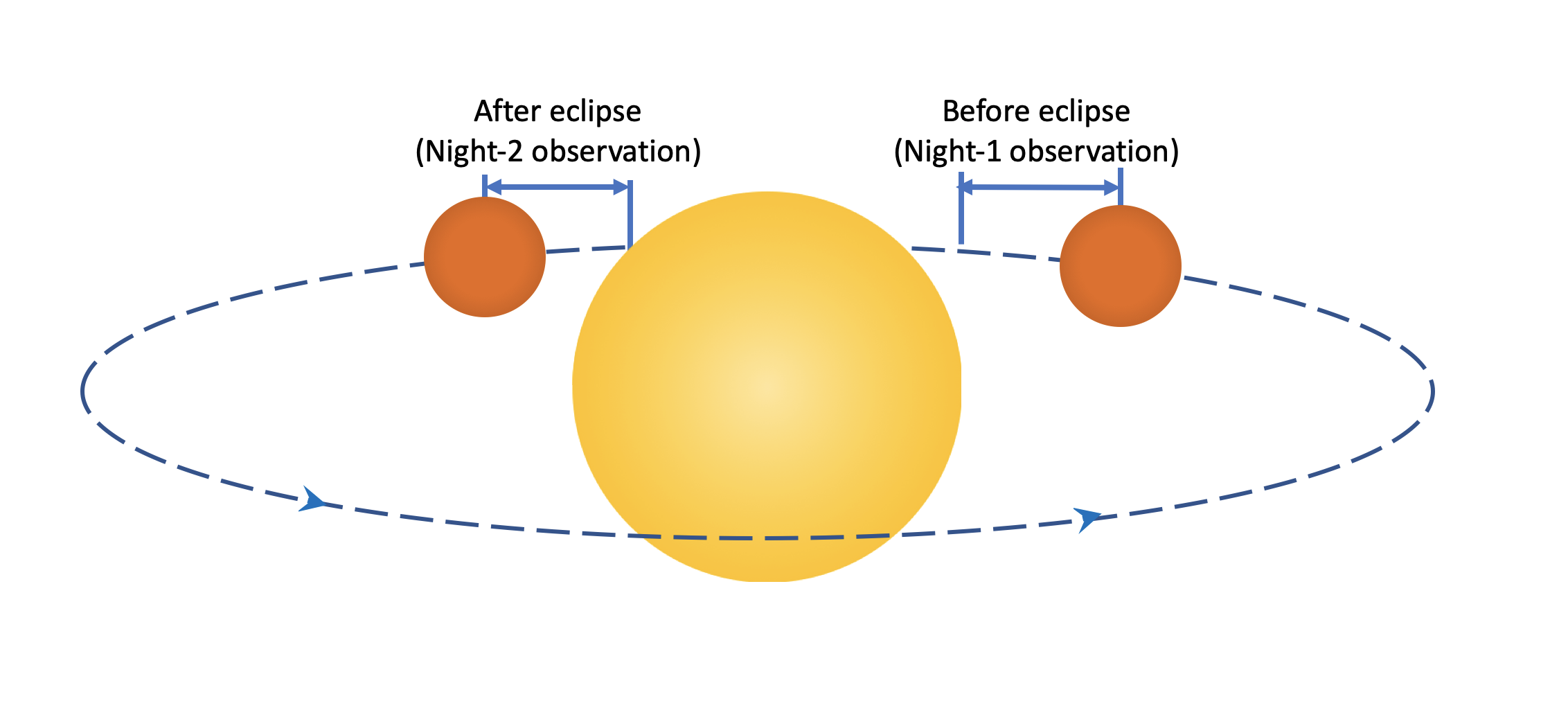
Figure 1: Schematic of the thermal emission observations. The orbital phase coverage of the two nights of observations is also indicated. The figure is not to scale.

The raw spectra were reduced with the CARMENES pipeline CARACAL v2.20 (Zechmeister et al. 2014; Caballero et al. 2016). The pipeline produces wavelength solutions that are obtained from the calibration lamps. These wavelength solutions are normally precise enough for detecting exoplanet atmospheres. For example, Alonso-Floriano et al. (2019) found that the CARMENES wavelengths drift during the night is about 15 m/s, which is negligible for exoplanet atmosphere observations. Therefore, we did not apply any further wavelength correction. The pipeline provides one-dimensional spectra with 61 spectral orders in the observatory rest frame along with a noise estimate for each data point. The detailed noise estimation of the pipeline was described by Zechmeister et al. (2014). We used the original wavelength sampling provided by the pipeline. We normalized the spectra order by order using a seventh-order polynomial fit.

We removed the telluric and stellar lines using the SYSREM algorithm (Tamuz et al. 2005; Birkby et al. 2013). The input data for SYSREM are the normalized order-by-order spectral matrix. The SYSREM algorithm also requires the noise of each data point. We used the noise value from the pipeline and applied error propagation to obtain the noise of the normalized spectrum. To preserve the relative depths of the planetary spectral lines, we applied the method proposed by Gibson et al. (2020). We first performed the SYSREM iterations in flux-space and instead of subtracting the input data with the SYSREM model, we then divided the input data by the SYSREM model. With this procedure, we preserved the strength of the planetary spectral lines at locations of the stellar and telluric absorption lines. The SYSREM procedure was performed on each spectral order separately. We tested different SYSREM iteration numbers (1 to 10) for the data set of the two nights. The final results do not change significantly after the first two iterations (cf. Fig. 3). We chose to use two iterations for night 1 and six iterations for night 2 because the final detection significance is highest at these iterations. The output spectra from SYSREM were then shifted into the stellar rest frame by correcting for the stellar systemic velocity (–24.48 km s^-1, Rainer et al. 2021) and the observer’s barycentric radial velocity (RV) of Earth. To further remove any broadband features in the residual spectrum, we filtered the spectra using a Gaussian high-pass filter with a Gaussian $\sigma$ of 15 points ($\sim$ 19 km s^-1). These final residual spectra were used to search for planetary spectral lines. An example of the data reduction procedure is presented in Fig. 2.

Table 1: Observation logs.

	Date	Airmass change	Exposure time [s]	$N_{\mathrm{spectra}}$	Phase coverage	$S/N$ range
Night-1	2020-05-21	1.87–1.01	120	85	0.411–0.459	52-107
Night-2	2020-07-09	1.07–1.01–1.17	120	83	0.515–0.564	65-92

Table 2: Parameters of system KELT-20b/MASCARA-2b.

Parameter	Symbol [unit]	Value
The star
Effective temperature	$T_{\mathrm{eff}}[K]$	8980${}_{-130}^{+90}$ a
Radius	$R_{\star}$ [$R_{\odot}$]	1.60 $\pm$ 0.06 a
Mass	$M_{\star}$ [$M_{\odot}$]	1.89${}_{-0.05}^{+0.06}$ a
Systemic velocity	$v_{\mathrm{sys}}$ [km s-1]	–24.48 $\pm$ 0.04 b
The planet
Radius	$R_{\mathrm{p}}$ [$R_{\mathrm{J}}$]	1.83 $\pm$ 0.07 a
Mass	$M_{\mathrm{p}}$ [$M_{\mathrm{J}}$]	¡ 3.51 c
Surface gravity	log $g$ [log cgs]	¡ 3.42 c
Orbital period	$P$ [d]	$3.4741070\pm{0.0000019}$ c
Transit epoch (BJD)	$T_{\mathrm{0}}$ [d]	$2457503.12005\pm{0.00019}$ c
Transit duration	$T_{\mathrm{14}}$ [d]	$0.14898\pm{0.0009}$ c
RV semi-amplitude	$K_{\mathrm{p}}$ [km s-1]	175.5${}_{-2.3}^{+2.8}$ a
		169.3${}_{-6.9}^{+8.9}$ c

Figure 2: Example of the data reduction procedure. These are the spectra from the first observation night, which are presented in a small wavelength range for demonstration purposes. The spectral matrices from top to bottom are original spectra, normalized spectra, spectra after the first SYSREM, spectra after the second SYSREM, spectra after the Gaussian high-pass filtering, and spectra after the masking. To estimate the efficiency of each data reduction procedure, we computed a metric $Q$, which is defined as the ratio of the mean value and the standard deviation of each spectral matrix.

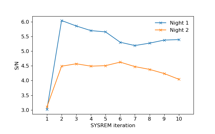
Figure 3: Evolution of the detection significance (i.e., S/N at the best-fit $K_{\mathrm{p}}$-$\mathrm{\Delta}\varv$ location) with different SYSREM iteration numbers.

3 Results and discussions

3.1 Detection of Fe emission lines

Because Fe i has relatively strong and dense emission lines in the CARMENES wavelength range, it is an ideal chemical species for emission spectroscopy observations. To search for the Fe i lines in the thermal emission spectrum, we cross-correlated the observed spectrum with a theoretical template spectrum (Snellen et al. 2010).

3.1.1 Cross-correlation method

We calculated the template spectrum similarly as described in Yan et al. (2020). We assumed a two-point parameterized temperature-pressure ($T$-$P$) profile (Brogi et al. 2014). At altitudes above the lower pressure point ($T_{\mathrm{1}}$, $P_{\mathrm{1}}$) and below the higher pressure point ($T_{\mathrm{2}}$, $P_{\mathrm{2}}$), the atmosphere was assumed to be isothermal, while between the two points, the temperature was assumed to change linearly with log $P$. According to theoretical simulations by Lothringer & Barman (2019), the two-point model is analogous to the temperature profiles of UHJs around hot stars. For the case of KELT-20b, we set the two points as (4500 K, $10^{-4}$ bar) and (2000 K, $10^{-2}$ bar) (Fig.4). This $T$-$P$ profile has a strong temperature inversion and is a reasonable approximation to the $T$-$P$ profiles from theoretical simulations (e.g., Lothringer & Barman 2019). We also assumed solar metallicity and set a constant mixing ratio of Fe i ($10^{-4.59}$). Because the mass of the planet is not well determined and only an upper limit has been reported in the discovery paper (Table 4), we assumed a surface gravity (log $g$) of 3.0 for the template calculation. We then used the petitRADTRANS tool (Mollière et al. 2019) to calculate the thermal emission spectrum of the planet ($F_{\text{p}}$) and obtained the stellar spectrum ($F_{\text{s}}$, assumed to be a blackbody spectrum). The high-resolution mode of petitRADTRANS provides spectra with a resolution of $10^{6}$. The observed spectrum of the star and planet system should be $F_{\text{p}}$+$F_{\text{s}}$. However, because the final observed spectrum is normalized, we expressed the template spectrum as 1 + $F_{\text{p}}$/$F_{\text{s}}$. We then normalized this template spectrum by dividing it with the continuum to remove the planetary continuum spectrum. The template was further convolved with the instrumental profile using the broadGaussFast code from PyAstronomy (Czesla et al. 2019). Here we used a Gaussian profile corresponding to the instrumental resolution of 94 600, which is measured from the calibration lamps by the CARMENES consortium team. Fig. 4 presents the final normalized and convolved template spectrum. We subsequently generated a grid of the template spectrum by shifting the spectrum from – 500 km s^-1 to + 500 km s^-1 in 1 km s^-1 steps with a linear interpolation. The actual wavelength sampling of the instrument ranges from 1.0 km s^-1 to 1.5 km s^-1, so the 1 km s^-1 step is a good approximation with a slight oversampling. We also filtered the template spectra with a Gaussian high-pass filter in the same way as was applied to the observed data, although this filtering process modifies the model spectra only slightly.

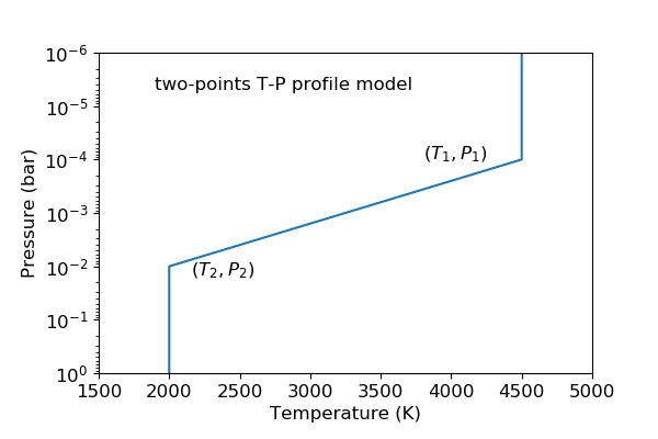
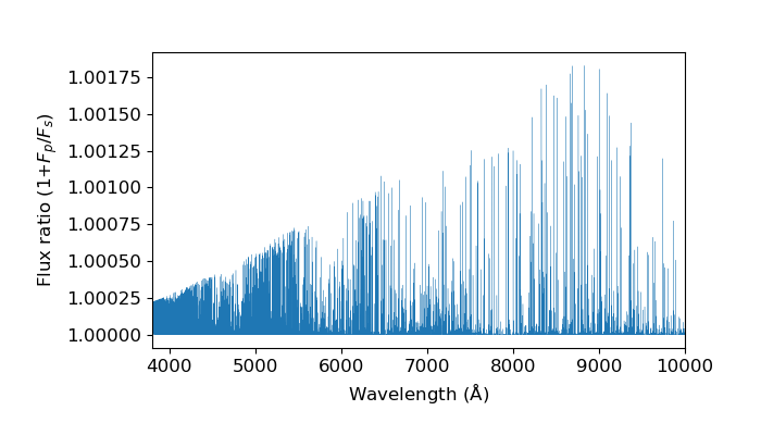
Figure 4: Two-point $T$-$P$ profile for the template spectrum calculation (top). Calculated thermal emission spectrum of Fe i (bottom). This template spectrum was used for the cross-correlation.

Before performing the cross-correlation, we masked the wavelength points with a low signal-to-noise ratio (S/N). We calculated an average S/N spectrum of all the observed spectra for each night and masked the wavelength points with S/N ¡ 50 for night 1 and S/N ¡ 40 for night 2. In this way, the strong telluric absorption lines were masked out. In addition, we excluded the data points at wavelengths below 545 nm and above 892 nm, considering that the spectrum has low S/Ns or strong telluric absorption lines at these wavelengths. We then computed the cross-correlation function (CCF) of each residual spectrum by cross-correlating the spectrum with the template grid.

3.1.2 Results of the cross-correlation

The obtained CCFs of the two nights spectra are presented in Fig.5. The upper panel of the figure is the CCF-map in the stellar rest frame and the atmospheric signature is the bright stripe with positive RV before eclipse and negative RV after eclipse, reflecting the planetary orbital motion. We further modeled the CCF map using the same method as Yan et al. (2020). We assumed that the CCF has a Gaussian profile and that the peak of the CCF is located at $K_{\mathrm{p}}\mathrm{sin(2\pi}\phi)+\mathrm{\Delta}\varv$, where $K_{\mathrm{p}}$ is the semi-amplitude of the planetary orbital RV, $\mathrm{\Delta}\varv$ is the RV deviation from the orbital motion, and $\phi$ is the orbital phase (phase 0 represents mid-transit). We set the width and height of the Gaussian profile as free parameters. We conducted Markov chain Monte Carlo (MCMC) simulations with the emcee tool (Foreman-Mackey et al. 2013) to sample from the posterior. The noise of each CCF was assigned as its standard deviation. The MCMC calculation was performed on the whole CCF matrix without the secondary eclipse data. The best-fit CCF-map is presented in the middle panel of Fig. 5. The MCMC yields estimates of $176.7\pm 0.6$ km s^-1 for $K_{\mathrm{p}}$ and $1.0\pm 0.2$ km s^-1 for $\mathrm{\Delta}\varv$. The small $\mathrm{\Delta}\varv$ could be a signature of atmospheric dynamics, but it could also originate from the uncertainties of the stellar systemic RV and planetary orbital ephemeris, which typically produce a change of $\mathrm{\Delta}\varv$ of several km s^-1 (Yan et al. 2020). The bottom panel of Fig.5 presents the CCFs shifted to the planetary rest frame using the best-fit $K_{\mathrm{p}}$ value.

The best-fit $K_{\mathrm{p}}$ is consistent with the theoretical values within $2\sigma$ (cf. Table 2). These values were calculated using the equation

$$K_{\mathrm{p}}=(2\mathrm{\pi}G\cdot M_{\star}/P)^{1/3}\cdot\mathrm{sin}\,i_{\mathrm{p}},$$ (1)

where $G$ is the gravitational constant, $P$ is the orbital period, $M_{\star}$ is the stellar mass, and $i_{\mathrm{p}}$ is the orbital inclination. On the other hand, the well-determined $K_{\mathrm{p}}$ value from planetary emission spectroscopy can be used to calculate the mass of the star. Using the above equation, we obtained $M_{\star}=2.00\pm 0.02M_{\odot}$, which is slightly higher than the literature values inferred from theoretical stellar evolution models: $1.89_{-0.05}^{+0.06}M_{\odot}$ (Talens et al. 2018) and $1.76_{-0.14}^{+0.19}M_{\odot}$ (Lund et al. 2017). This demonstrates that emission spectroscopy is a unique tool for independently measuring stellar mass. This was initially proposed and demonstrated by de Kok et al. (2013).

We also computed the classical $K_{\mathrm{p}}$-$\mathrm{\Delta}\varv$ maps for the individual nights and the combined data (Fig.6). The maps were generated by adding up the CCFs in the planetary rest frame with different $K_{\mathrm{p}}$ values. To estimate the significance of the detection, we computed the standard deviation of the CCFs within the $\left|\mathrm{\Delta}\varv\right|$ range between 100 and 200 km s^-1, and took this value as the noise of the map. The detection significance of night 1 is higher than that of night 2. The $K_{\mathrm{p}}$-$\mathrm{\Delta}\varv$ map of the combined data shows a clear peak (S/N $\sim$ 7.7) located around $K_{\mathrm{p}}$ = $177$ km s^-1 and $\mathrm{\Delta}\varv$ = $1.0$ km s^-1.

The detection of Fe i emission lines in the thermal emission spectrum of KELT-20b is unambiguous evidence for a thermal inversion layer in its dayside atmosphere. KELT-20b is the fourth planet in which Fe i emission lines are detected on the planetary dayside hemisphere, after KELT-9b, WASP-189b, and WASP-33b (Pino et al. 2020; Yan et al. 2020; Nugroho et al. 2020a; Cont et al. 2021). These four planets are all UHJs orbiting A-type stars, indicating that hot stars can create strong temperature inversion, which makes the Fe i emission lines relatively strong. This scenario is consistent with the simulation by Lothringer & Barman (2019), who proposed that the temperature and slope of the inversion layer increase with stellar effective temperature because of the enhanced absorption at short wavelengths and low pressures.

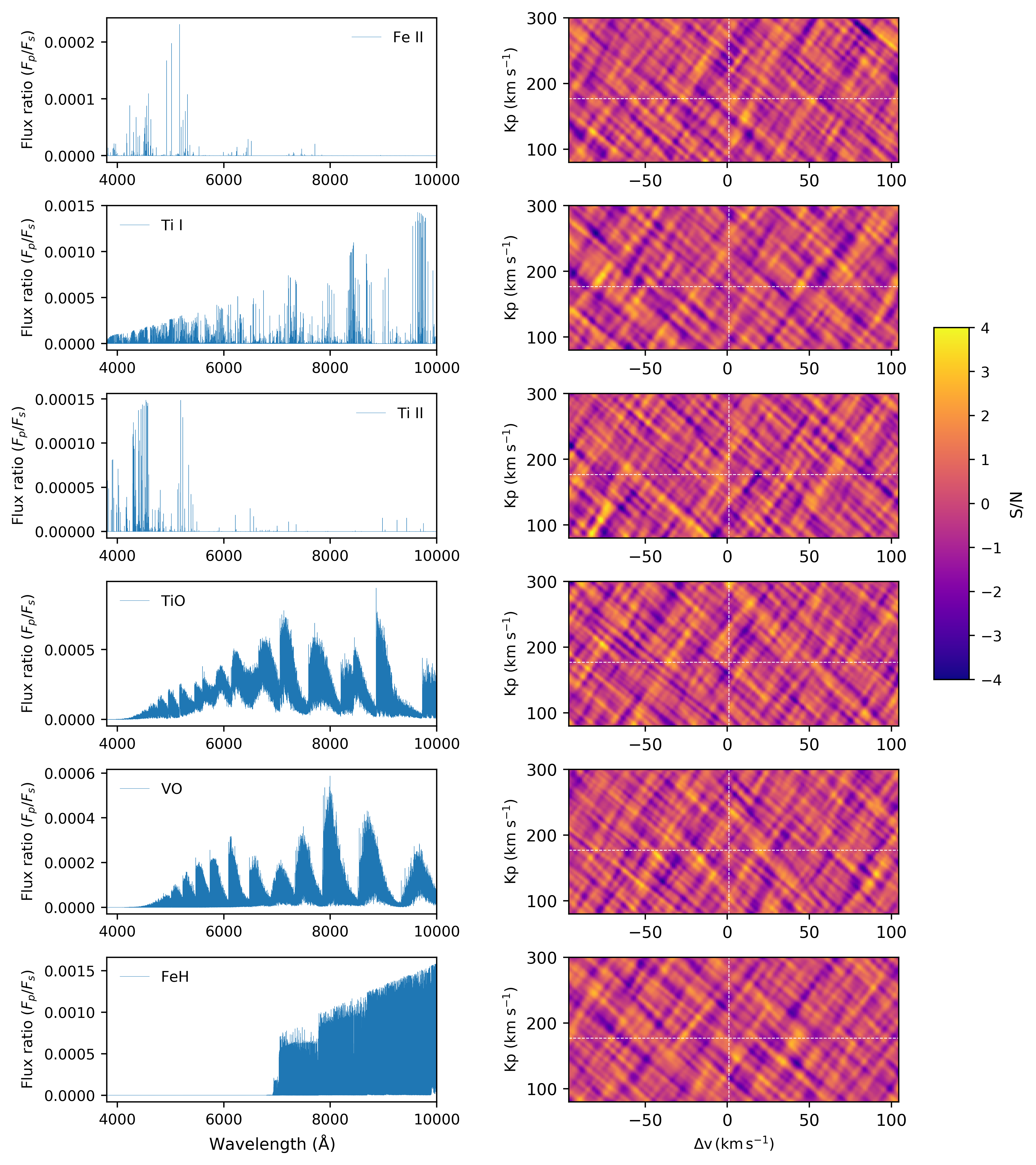
Figure 9: Nondetection of several other chemical species. Left panels: Spectral model of each species. These are normalized spectra that are calculated in a similar way as described in Section 3.1.1. Right panels: Combined two-night $K_{\mathrm{p}}$-$\mathrm{\Delta}\varv$ map of each species. The dashed white lines indicate the location of the best-fit $K_{\mathrm{p}}$-$\mathrm{\Delta}\varv$ from the Fe i signal.

In addition to Fe i, we also searched for other species, including Fe ii, Ti i, Ti ii, TiO, VO, and FeH. However, we were not able to detect them (cf. Fig. 9). The nondetection of these species could be due to several reasons, for example, relatively weak emission lines in the CARMENES wavelength range, a poor accuracy of the line lists, an insufficient S/N of the data, or the nonexistence of the species in the temperature inversion layer. The detection of the strong Fe i feature benefits from the high-accuracy line list and the large number of spectral lines covering a wide wavelength range.

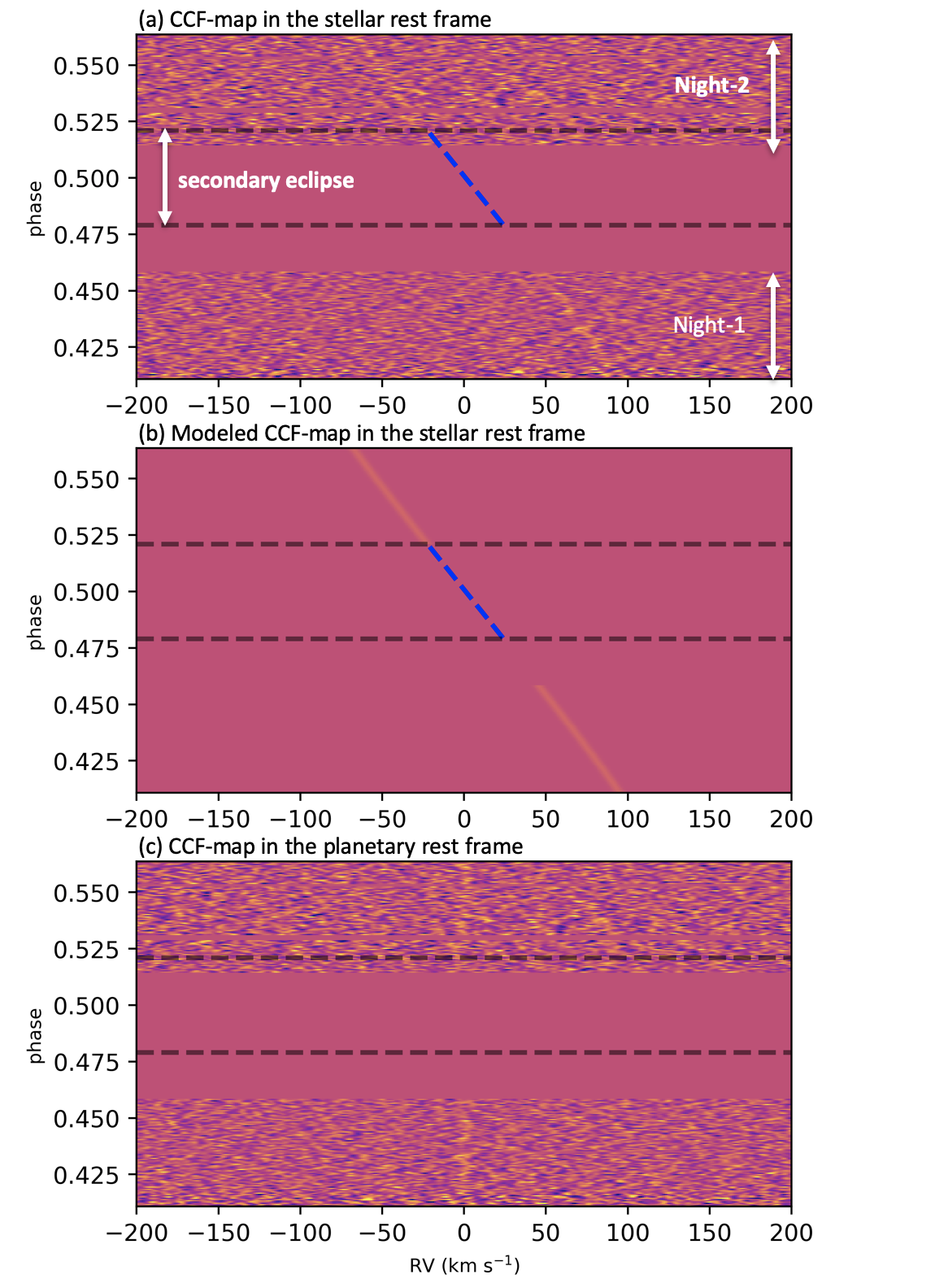
Figure 5: Cross-correlation functions of the spectra from the two nights. Upper panel: CCF map in the stellar rest frame. Middle panel: Modeled CCF map with the best-fit $K_{\mathrm{p}}$ and $\mathrm{\Delta}\varv$ values. Lower panel: CCF map in the planetary rest frame. The horizontal dashed lines indicate the beginning and end of the eclipse. The dashed blue line denotes the planetary orbital motion RV.

Figure 6: Combined cross-correlation functions with different $K_{\mathrm{p}}$ values (i.e., $K_{\mathrm{p}}$-$\mathrm{\Delta}\varv$ map). Panels a, b, and c: Maps of night 1, night 2, and the combination of the two nights, respectively. The dashed white lines indicate the location of the best-fit $K_{\mathrm{p}}$ and $\mathrm{\Delta}\varv$ values (i.e., 177.5 km s^-1 and 1.0 km s^-1). Panel d: CCF at the best-fit $K_{\mathrm{p}}$.

3.1.3 Differences between the results of the two nights

We observed the thermal emission spectrum during two nights, before eclipse for the first night and after eclipse for the second night (Fig.1). The cross-correlation results (i.e., CCF and $K_{\mathrm{p}}$ map) of each night are presented in Fig.5 and Fig.6. There are some differences between the $K_{\mathrm{p}}$ maps of the two nights. The maximum S/N (6.4 $\sigma$) for night 1 is located at $K_{\mathrm{p}}$ = $176.4\pm 4$ km s^-1 and $\mathrm{\Delta}\varv$ = $1.2_{-1.6}^{+1.7}$ km s^-1, which is consistent with the expected $K_{\mathrm{p}}$. However, the maximum S/N (5.7 $\sigma$) for night 2 is located at $K_{\mathrm{p}}$ = $152.4\pm{3.2}$ km s^-1 and $\mathrm{\Delta}\varv$ = $-9.5\pm{0.9}$ km s^-1, deviating from the expected values. This difference means that the RVs of the detected Fe i emission lines deviate by several km s^-1 from the orbital motion. This deviation might be the result of atmospheric dynamics such as rotation and winds. In addition, the signal from the before-eclipse observation is slightly stronger than that from the after-eclipse observation. This asymmetry feature might be due to an eastward hotspot offset, which causes the average temperature of the visible hemisphere during the before-eclipse observation to be higher than that during the after-eclipse observation. However, the poor S/N of the second night is not sufficient to draw any conclusions about the nature of dynamics in the atmosphere. Further observations with higher S/N in combination with general circulation models should be able to confirm or discard this hypothesis.

In addition to the emission spectroscopy, Fe i has also been detected in the transmission spectrum of KELT-20b. The Fe i transmission spectrum is blueshifted by 5 - 10 km s^-1 and the signal has an asymmetric feature between the first and second half of the transit (Stangret et al. 2020; Nugroho et al. 2020b; Hoeijmakers et al. 2020; Rainer et al. 2021), probably caused by atmospheric dynamics.

3.2 Retrieval of atmospheric properties

3.2.1 Retrieval with CARMENES data

Techniques to retrieve the properties of exoplanet atmospheres from high-resolution spectroscopy have been developing in recent years (e.g., Brogi & Line 2019; Gandhi et al. 2019; Shulyak et al. 2019; Gibson et al. 2020). To retrieve the atmospheric properties of KELT-20b from the observed Fe i emission lines, we applied the method described in Yan et al. (2020) with the following steps:
(1) Calculating a master residual spectrum. Because $K_{\mathrm{p}}$ and $\mathrm{\Delta}\varv$ are well determined with our data, we fixed these two parameters and shifted all the residual spectra by correcting the planetary orbital RV and $\mathrm{\Delta}\varv$. Only the out-of-eclipse data were used. The master residual spectrum was then obtained by averaging these shifted residual spectra with the square of the S/N as the weight of each data point. This master residual spectrum is regarded as the normalized spectrum with no information about the spectral continuum, because we have already normalized the original spectra and removed the broad features when we performed the SYSREM and Gaussian filtering described in Section 2.
(2) Setting up the spectral model. We used the petitRADTRANS tool to forward-model the dayside spectrum. The $T$-$P$ profile was parameterized using the two-point model. The atmosphere model consisted of 25 layers that were uniformly spaced in log($P$) ranging from 1 bar to $10^{-8}$ bar. We used an opacity grid of Fe i up to 25 000 K. For a given $T$-$P$ profile, the mixing ratio of Fe i was computed with the chemical equilibrium module easyCHEM of petitCode (Mollière et al. 2015, 2017). We also set the elemental abundance to solar and log $g$ to 3.0. The simulated thermal emission spectrum of Fe i (1 + $F_{\text{p}}$/$F_{\text{s}}$) was normalized, convolved, interpolated, and filtered in the same way as described in Section 3.1.
(3) Fitting the master residual spectrum with the spectral model. Following Yan et al. (2020), we assumed a standard Gaussian likelihood function expressed in logarithm,

$$\mathrm{ln}(L)=-\frac{1}{2}\sum_{i}\left[\frac{(R_{i}-m_{i})^{2}}{(\beta\sigma_{i})^{2}}+\mathrm{ln}(2\pi(\beta\sigma_{i})^{2})\right],$$ (2)

where $R_{i}$ is the observed master residual spectrum at wavelength point $i$, $m_{i}$ is the spectral model, $\sigma_{i}$ is the uncertainty of the observed spectrum, and $\beta$ is a uniform scaling term of the uncertainty. We then applied the MCMC method to obtain the best-fit parameters and their uncertainties by evaluating the likelihood function with the emcee tool. The MCMC calculation had 5000 steps with 24 walkers. We set uniform priors for the parameters with the boundary conditions shown in Table 3.

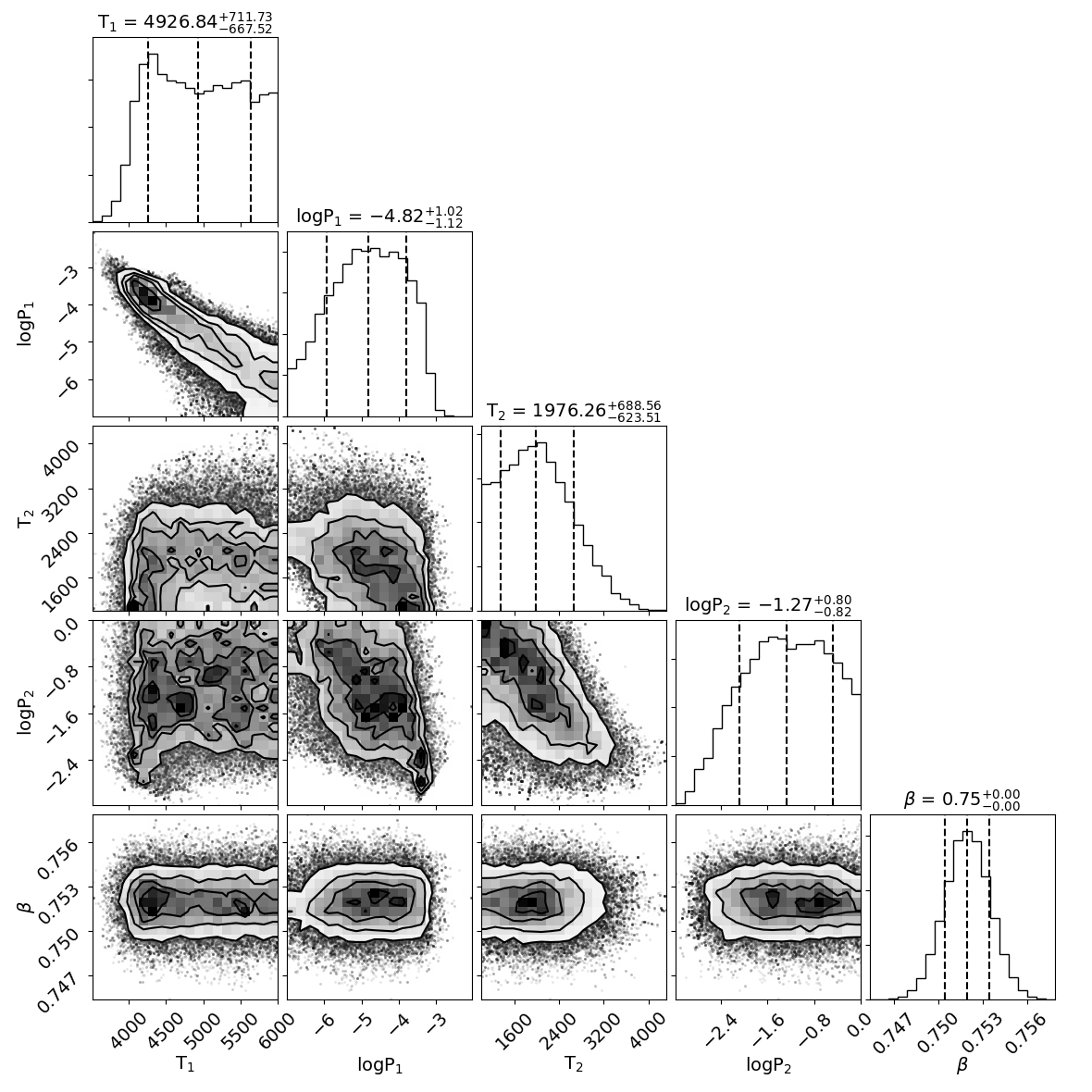
Figure 10: Posterior distribution of the parameters from the MCMC fit of the CARMENES data. Here both $\mathrm{log}\,g$ and [Fe/H] are fixed.

The retrieved parameters are summarized in Table 3 and the best-fit $T$-$P$ profile is presented in Fig.7. The posterior distributions are plotted in Fig.10. The retrieved result indicates that the planet has a steep temperature inversion with very high temperatures ($\sim$ 4900 K) in the upper layer.

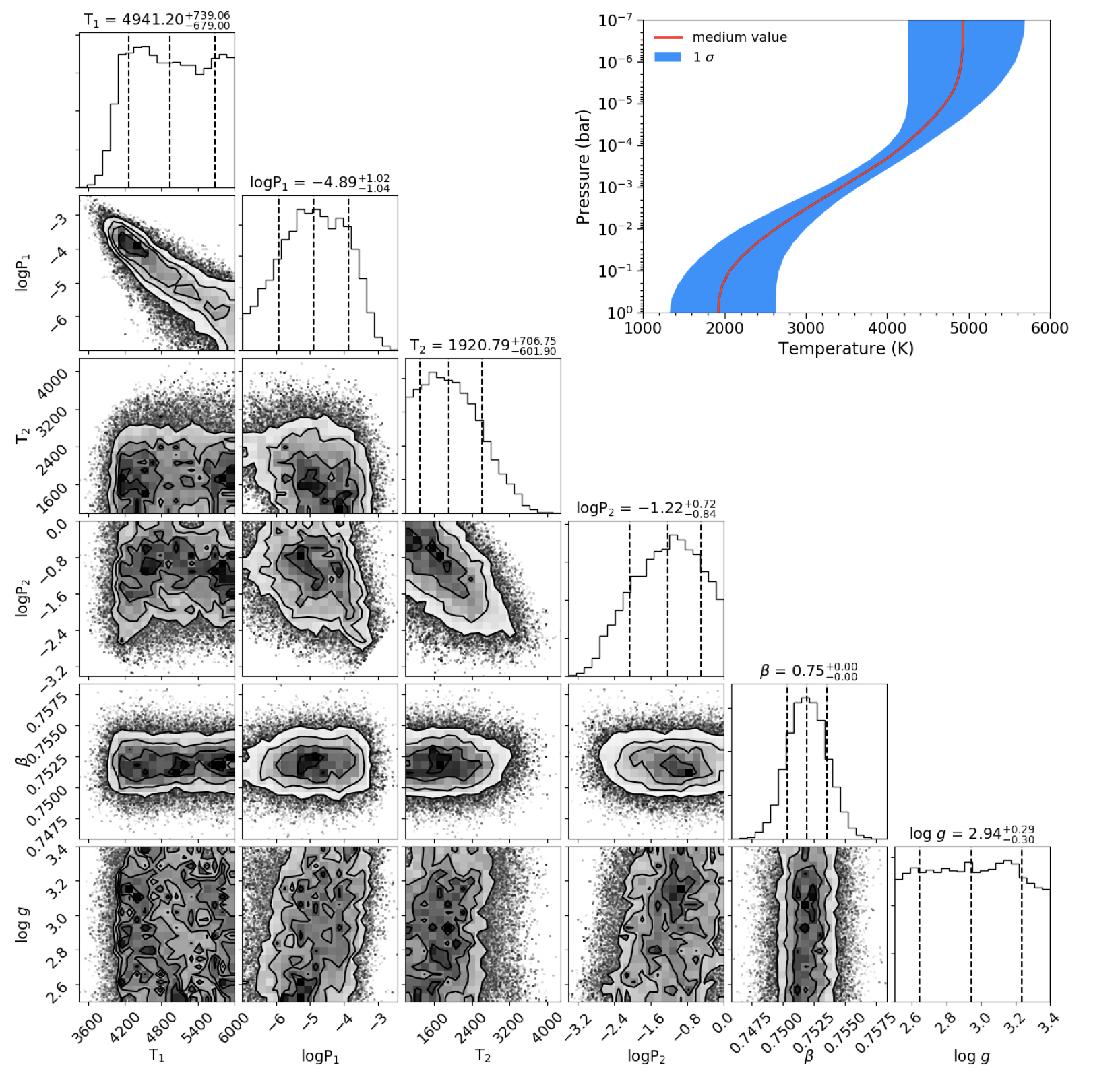
Figure 11: Same as Fig.10, but with $\mathrm{log}\,g$ as a free parameter. The inset shows the retrieved $T$-$P$ profile.

In this retrieval, we assumed a solar elemental abundance for Fe and set log $g$ to 3.0. However, the retrieved $T$-$P$ profile depends on the Fe elemental abundance and on surface gravity. We tested different abundances and surface gravity values and found that these two parameters mostly affect the location (i.e., $P_{\mathrm{1}}$ and $P_{\mathrm{2}}$) of the inversion, while the temperature is less affected. With a higher elemental abundance or a lower surface gravity, the retrieved inversion layer is located at higher altitudes. We performed the retrieval with log $g$ as a free parameter with an upper boundary of 3.4 and lower boundary of 2.5. The retrieved results indicate that the $T$-$P$ profile is heavily degenerate with log $g$ (Appendix Fig.11) and the data constrain log $g$ only poorly. Future RV follow-up observations will be useful in constraining the planetary mass and the planetary surface gravity.

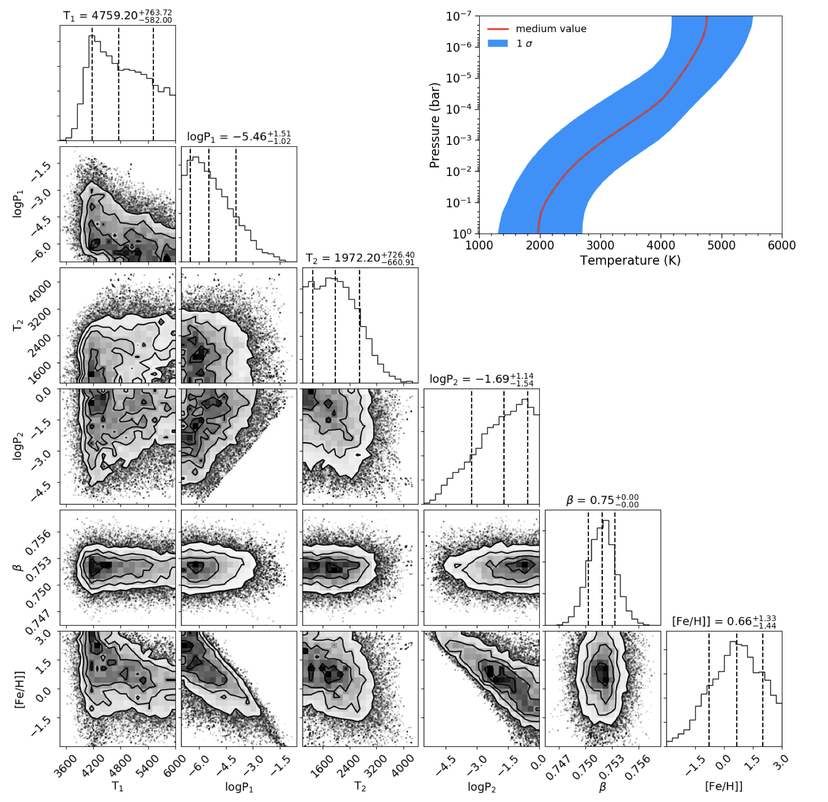
Figure 12: Same as Fig.10, but with [Fe/H] as a free parameter. The inset shows the retrieved $T$-$P$ profile.

We also performed the retrieval with the Fe elemental abundance ([Fe/H]) as a free parameter. For a given [Fe/H] value, we calculated the mixing ratio of Fe i using easyCHEM. The retrieved [Fe/H] is $0.7_{-1.4}^{+1.3}$ dex (Table 7 and Fig.12). The large error of the retrieved value indicates that there is a certain degree of degeneracy between [Fe/H] and the $T$-$P$ profile. In addition, Fossati et al. (2021) found that nonlocal thermodynamic equilibrium (NLTE) can affect the upper atmosphere of UHJs. NLTE effects at low pressures can alter the Fe level population and thereby affect the retrieval of the Fe abundance and $T$-$P$ profile. Detection of other species (e.g., Fe ii and FeH) and inclusion of the NLTE effects in the retrieval will enable us to better constrain the Fe abundance.

Table 3: Best-fit parameters from the $T$-$P$ profile retrieval.

Parameter	Value	Value (TESS included)	Value ([Fe/H] free)	Value (log $g$ free)	Boundaries	Unit
$T_{\mathrm{1}}$	$4900\pm{700}$	$4900_{-600}^{+700}$	$4700_{-600}^{+800}$	$4900\pm{700}$	1000 to 6000	K
log $P_{\mathrm{1}}$	$-4.8_{-1.1}^{+1.0}$	$-5.0_{-1.1}^{+1.0}$	$-5.5_{-1.0}^{+1.5}$	$-4.9\pm{1.0}$	$-7$ to 0	log bar
$T_{\mathrm{2}}$	$1900_{-600}^{+700}$	$2550_{-250}^{+150}$	$2000\pm{700}$	$1900_{-600}^{+700}$	1000 to 6000	K
log $P_{\mathrm{2}}$	$-1.3\pm{0.8}$	$-1.5_{-0.6}^{+0.7}$	$-1.7_{-1.5}^{+1.1}$	$-1.2_{-0.8}^{+0.7}$	$-7$ to 0	log bar
$\beta$	$0.752\pm{0.0015}$	$0.752\pm{0.0015}$	$0.752\pm{0.0015}$	$0.752\pm{0.0015}$	0 to 10	…
[Fe/H]	0 (fixed)	0 (fixed)	$0.7_{-1.4}^{+1.3}$	0 (fixed)	$-3$ to +3	dex
log $g$	3.0 (fixed)	3.0 (fixed)	3.0 (fixed)	$3.0\pm 0.3$	2.5 to 3.4	log in cgs

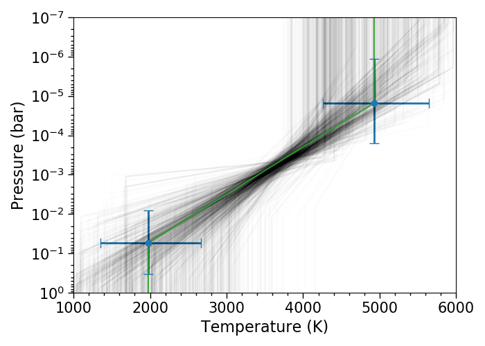
Figure 7: Retrieved $T$-$P$ profile from the CARMENES data. Upper panel: Retrieved results of the two-point $T$-$P$ model. The blue points with error bars are the best-fit ($T_{\mathrm{1}}$, $P_{\mathrm{1}}$) and ($T_{\mathrm{2}}$, $P_{\mathrm{2}}$) values. The gray lines show examples of the $T$-$P$ profiles sampled by the MCMC analysis. Lower panel: Median of the sampled $T$-$P$ profiles (red line) and the 1$\sigma$ envelope (blue shadow). They are generated by sorting the temperatures of the MCMC samples at each of the 25 atmosphere layers.

3.2.2 Joint retrieval with TESS data

The secondary eclipse of KELT-20b was recently measured by Wong et al. (2021) using the TESS light curve. The reported eclipse depth is $111_{-36}^{+35}$ ppm. This provides the spectral continuum level of the dayside hemisphere. Therefore, the TESS data are complementary to the high-resolution spectrum of the Fe i emission lines, which lacks the continuum information. We therefore included the TESS eclipse data point in our retrieval. First, we calculated the un-normalized $F_{\text{p}}$/$F_{\text{s}}$ spectrum, which contains both the continuum spectrum and the line spectrum. Then we integrated the flux spectrum using the rebin-give-width tool of petitRADTRANS from 0.6 $\mathrm{\mu}$m to 1.0 $\mathrm{\mu}$m, which is an approximation of the TESS bandpass. In this way, we obtained the modeled secondary eclipse depth. Subsequently, we calculated the likelihood function for the TESS data as

$$\mathrm{ln}(L_{\mathrm{T}})=-\frac{1}{2}\left[\frac{(R_{\mathrm{T}}-m_{T})^{2}}{\sigma_{\mathrm{T}}^{2}}+\mathrm{ln}(2\pi\sigma_{\mathrm{T}}^{2})\right],$$ (3)

where $R_{\mathrm{T}}$ is the modeled eclipse depth, $m_{\mathrm{T}}$ is the TESS measured eclipse depth (111 ppm), and $\sigma_{\mathrm{T}}$ is the noise (36 ppm). The subscript (T) denotes that these are parameters for the TESS calculation. This likelihood function was then added to the likelihood function of the CARMENES data (Eq. 2). To perform the joint retrieval, we applied the MCMC calculations to this combined likelihood function in the same way as for the CARMENES-only retrieval.

The jointly retrieved values are presented in Table 3 and the $T$-$P$ profile envelope is plotted in Fig. 8. The TESS data mostly constrain the cooler low-altitude layers of the atmosphere in which the continuum spectrum originates, therefore, the $T_{\mathrm{2}}$ value ($2550_{-250}^{+150}$ K) is better determined than the result of CARMENES-only data (cf. the posterior distribution plot in Fig.13).

In the retrieval, we only included the blackbody thermal emission as the continuum source. However, $\mathrm{H^{-}}$ has been proposed as an important continuum source for UHJs (e.g., Parmentier et al. 2018). Therefore, we estimated the impact of $\mathrm{H^{-}}$ on the retrieval. We took the best-fit parameters from the retrieval and compared the modeled spectra with and without $\mathrm{H^{-}}$. For the TESS secondary eclipse of KELT-20b, the $\mathrm{H^{-}}$ contribution is $\sim$ 10 ppm, which is within the noise level of the measured eclipse depth. For the strength of the Fe emission line, $\mathrm{H^{-}}$ has a negligible contribution (Yan et al. 2020).

We assumed that the measured dayside flux arises from the thermal emission. However, reflected light can also contribute to the measured TESS eclipse depth (e.g., Daylan et al. 2021; von Essen et al. 2021). Because of the degeneracy between the reflected flux and the thermal emission flux, the TESS data alone cannot constrain the geometric albedo ($A_{\mathrm{g}}$) of KELT-20b (Wong et al. 2021). Nevertheless, measurements of other UHJs suggest that their albedos are very low (e.g., Bell et al. 2017; Shporer et al. 2019; Wong et al. 2021). To estimate the strength of possible reflected light, we followed the method described by Alonso (2018) and calculated the light contribution to $F_{\text{p}}$/$F_{\text{s}}$ as $A_{\mathrm{g}}$ $R_{\mathrm{p}}^{2}/a^{2}$. When assuming $A_{\mathrm{g}}$ = 0.1, we obtained a value of 24 ppm, which is within the noise level of the TESS result.

3.2.3 Comparison with self-consistent models

To compare the retrieved $T$-$P$ profile with self-consistent models, we calculated $T$-$P$ profiles using the HELIOS code originally presented in Malik et al. (2017). We used an updated version of HELIOS, which includes opacities due to neutral and singly ionized species as described in Fossati et al. (2021). In particular, we included atomic line opacities due to neutral and singly ionized atoms, namely C i-ii, Cr i-ii, Fe i-ii, K i-ii, Mg i-ii, Na i-ii, O i-ii, and Si i-ii, which are found to contribute most to the line opacity throughout the planetary atmosphere. The original line lists are those produced by R. Kurucz (Kurucz 2018). The molecular line opacity includes molecules such as CH₄, CO₂, CO, H₂O, HCN, NH₃, OH, SiO, TiO, and VO. The pretabulated cross sections of these molecules were taken from the public opacity database for exoplanetary atmospheres. We also extended continuum opacity sources by including, for example, continuum transitions of H^-, He^-, and metals (see Fossati et al. 2020, 2021). The HELIOS calculations were performed assuming local thermodynamic equilibrium.

We assumed solar abundance, log $g$ = 3.0, and zero albedo to compute the atmosphere of KELT-20b. We calculated two extreme cases: one case with full heat redistribution from the dayside to nightside (corresponding to a dayside $T_{\mathrm{eq}}$ of 2300 K), and the other case without heat redistribution (corresponding to dayside $T_{\mathrm{eq}}\sim 3000\,K$). In addition, we calculated the models with an atmosphere without TiO. The modeled $T$-$P$ profiles are presented in Fig. 8.

All of these self-consistent models predict the existence of a temperature inversion layer. The contribution of TiO to the temperature inversion is relatively weak, especially for the $T_{\mathrm{eq}}$ $\sim$ 3000 K case. The retrieved temperature inversion layer is located between the two heat redistribution cases, especially at pressures of $10^{-3}-10^{-4}$ bar, where the Fe emission line cores are formed. This means that our retrieved $T$-$P$ profile is consistent with the self-consistent models because the actual heat redistribution is expected to be in between the two extreme cases.

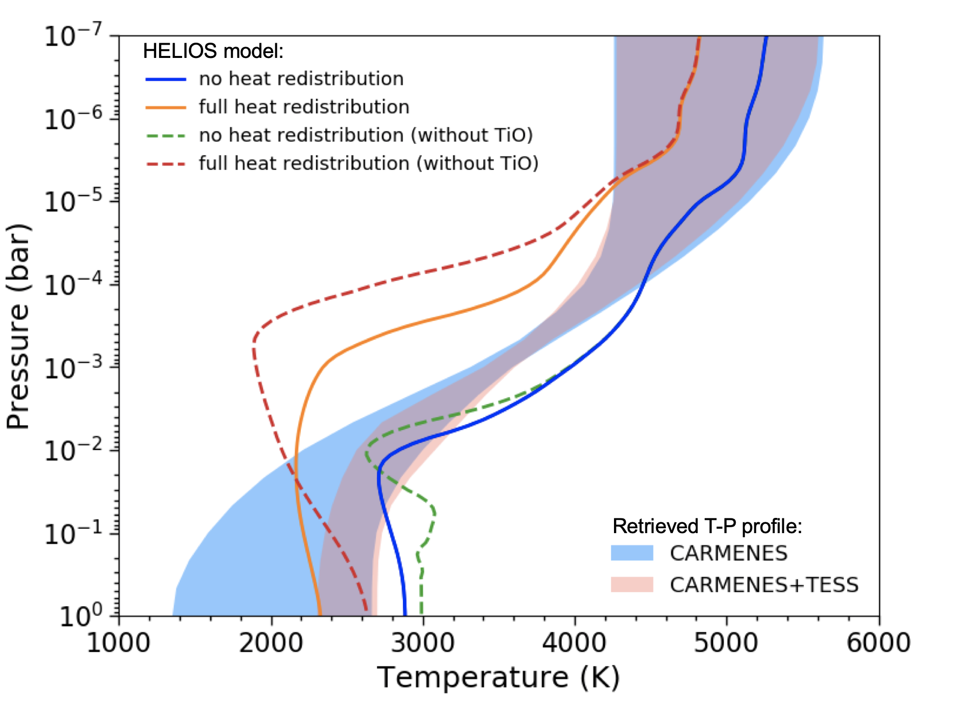
Figure 8: Comparison between the theoretical $T$-$P$ profile from the self-consistent HELIOS model and the retrieved $T$-$P$ profile from the CARMENES and TESS observations. The solid lines are the HELIOS results assuming no heat redistribution or full heat redistribution from the dayside to nightside. The dashed lines are the models without TiO. The 1$\sigma$ range of the retrieved $T$-$P$ profiles is indicated as the blue shadow (CARMENES data) and the salmon shadow (CARMENES + TESS data).

4 Conclusions

We observed the dayside thermal emission spectrum of the ultra-hot Jupiter KELT-20b with the CARMENES spectrograph. The observation covers planetary orbital phases before and after the secondary eclipse. We employed the cross-correlation technique to search for atmospheric species in the planetary dayside hemisphere and detected a strong neutral Fe signal. The detected Fe lines are in emission, which unambiguously indicates the existence of a temperature inversion layer in the atmosphere. So far, temperature inversion has been detected in four UHJs (i.e., KELT-9b, WASP-33b, WASP-189b, and KELT-20b) using high-resolution thermal emission spectroscopy. The detection of temperature inversion is consistent with theoretical simulations that predict its existence.

We retrieved the atmospheric profile with the observed high-resolution Fe i emission lines in KELT-20b using the petitRADTRANS forward model and the easyCHEM chemical equilibrium code. The results show a strong temperature inversion with a temperature around 4900 K at the upper layer of the inversion. In addition, we included the secondary eclipse depth that was recently measured with TESS (Wong et al. 2021). The joint CARMENES + TESS fit yields a tighter constraint on the temperature ($\sim$ 2550 K) of the lower-altitude atmosphere in which the photosphere is located. We also computed the self-consistent atmospheric structure using the code HELIOS, which shows $T$-$P$ profiles that are consistent with the retrieved result.

Ground-based high-resolution emission spectroscopy is a powerful technique for probing the dayside hemispheres of UHJs. Emission spectroscopy is particularly sensitive in characterizing the temperature structure (e.g., temperature inversion). In addition, the phase-resolved emission spectroscopy can be used to characterize atmospheric dynamics and the global distribution of temperature and chemical species.

Appendix A Additional figures

Figure 13: Same as Fig.10, but for the CARMENES+TESS data.